Ring solitons and soliton sacks in imbalanced fermionic systems
Abstract
We show that in superfluids with fermionic imbalance and uniform ground state, there are stable solitons. These solutions are formed of radial density modulations resulting in nodal rings. We demonstrate that these solitons exhibit nontrivial soliton-soliton and soliton-vortex interactions and can form complicated bound states in the form of “soliton sacks”. In a phase-modulating (Fulde-Ferrell) background, we find different solitonic states, in the form of stable vortex-antivortex pairs.
I Introduction
Solitons have long been understood to have profound consequences for the physical properties of fermionic systems Jackiw and Rebbi 1976; Heeger et al. 1988; Goldstone and Wilczek 1981; Yefsah et al. 2013. Recently new methods were developed to create and observe solitons in superfluid ultracold atoms Yefsah et al. 2013, opening up a route to explore new regimes and properties Lutchyn et al. 2011; Efimkin and Galitski 2015; Ku et al. 2016; Ren and Aleiner 2019; Dutta and Mueller 2017. We will focus on the existence of solitons in so-called imbalanced Bardeen-Cooper-Schrieffer (BCS) fermionic systems. Such superfluids exhibit pairing between fermions with different magnitudes of Fermi momenta. For example such pairing has been considered in the context of dense quark matter Alford et al. 2001, mixtures of different ultracold atoms Zwierlein et al. 2006; Radzihovsky 2011; Samoilenka et al. 2020a; Bulgac and Forbes 2008; Radzihovsky and Sheehy 2010; Son and Stephanov 2006, and superconductors Bianchi et al. 2003; Cho et al. 2017; Uji et al. 2018; Mayaffre et al. 2014; Coniglio et al. 2011; Norman 1993; Cho et al. 2011; Matsuda and Shimahara 2007; Lortz et al. 2007; Singleton et al. 2000; Martin et al. 2005; Agterberg et al. 2014; Barkman et al. 2019a. When the effects of imbalance are strong, the ground state of such a system can spontaneously break translation symmetry, by inducing periodic modulation in the complex order parameter. Two commonly considered inhomogeneous ground states are the Fulde-Ferrell (FF) state Fulde and Ferrell 1964, which exhibits purely phase modulation, and the Larkin-Ovchinnikov (LO) state Larkin and Ovchinnikov 1964, which consists of purely density modulation. These two are jointly referred to as FFLO states. Situations where both phase and density modulate, have also been found Barkman et al. 2019a; Samoilenka et al. 2020a. Conversely, if the imbalance is weak, the ground state remains uniform. In this paper, we will show that fermionic imbalance can nonetheless change the properties of the system, even when the ground state is uniform, through the existence of energetically stable solitonic excitations The.
II Ginzburg-Landau model
We consider imbalanced systems in the weak-coupling limit, close to the tricritical point, i.e., where the uniform, FFLO and normal phases meet. Near the tricritical point the amplitude of the order parameter and its gradients are small, justifying a Ginzburg-Landau (GL) free-energy expansion, which has been derived from the microscopic theory for various imbalanced systems Buzdin and Kachkachi 1997; Radzihovsky 2011; Agterberg and Yang 2001; Barkman et al. 2019a. Fermionic population imbalance diminishes the coefficient of the second-order gradient term, which leads to the required inclusion of higher-order gradient terms. We will use the GL model, originally derived in Buzdin and Kachkachi 1997, which has been shown to be sufficient when describing effects far from the boundary Barkman et al. 2019b; Samoilenka et al. 2020b, where the free-energy density reads
| (1) | |||
written in dimensionless units, where the field is the complex order parameter. The model applies for systems with pairing between electrically neutral fermions or superconductors where the coupling to the vector potential is negligible. The two parameters and are positive constants and, for systems with a two-dimensional Fermi surface, are given to be and . Therefore the model can be described by a single parameter , which depends on both the temperature and the population imbalance, fixed by the Zeeman splitting energy . The rescaled spatial coordinate is measured in units of the length scale , where is a dimensionless quantity that diverges as the tricritical point is approached. Here, denotes the Fermi velocity and denotes the critical temperature at no population imbalance. Details of the rescaling are presented in Appendix A.
Since the second-order gradient term is strictly negative, there exists the possibility of nonuniform ground states. This can be seen in the two-dimensional model, where the configuration that minimizes the free energy transitions from a uniform state , where , to a density-modulating LO state at . This inhomogeneous state minimizes the free energy until the transition to the normal state at . We note that the soliton solutions we find exist for the parameter region , which is comparable to the size of the LO regime. These values of can be translated into the corresponding values of the Zeeman splitting energy and the temperature , as seen in FIG. 1.

One feature to note regarding Eq. (1) is that it is mathematically related to the Swift-Hohenberg equation, which is also described by a fourth order partial differential equation. This model, initially formulated in the context of thermal convection Swift and Hohenberg 1977, is commonly used to model pattern formation. The main differences between the GL model described by Eq. (1) and the standard Swift-Hohenberg equation are that the order parameter is complex valued and there is an additional coupling between the field strength and the gradient in the terms proportional to in Eq. (1). A more detailed comparison between the models can be found in Appendix B.
III Ring solitons
We turn now to the numerical solutions of the free energy in Eq. (1). We used a nonlinear conjugate gradient flow method both in finite element (FREEFEM Hecht 2012) and finite difference schemes, which produced consistent results.
We find numerically that the two-dimensional GL free energy defined by the density in Eq. (1) has a number of local minima, in the form of solitons. The simplest subset of these soliton solutions retain the rotational spatial symmetry of the model, which we coin “ring solitons”. These radial solutions take the form , where is a constant and is a real profile function that modulates continuously between being positive and negative, before decaying to its ground-state value as . This leads us to characterise the solutions by the number of radial nodes () they exhibit (). In the cases where is constant, we assume without loss of generality that and thus is a real field. The solutions are displayed in FIG. 2, where changes sign once. It is important to note that the energy density deviation from the uniform state, plotted for in FIG. 2, decays such that the total soliton energy is finite. This means that since entropy scales with system size, solitons will be thermally induced in the thermodynamic limit.


We found stable solutions for , which suggests that a system with sufficiently weak imbalance will not support these solitonic excitations (see FIG. 1 for the conversion into dimensionful parameters). As increases, the size of the soliton also increases, and the order parameter approaches at the center of the soliton.
For higher values of we find that solutions become stable, first at for , followed by solutions with three and four nodal rings () at and respectively. The - solutions are plotted in FIG. 3 along with their energies and increasing nodal radii (i.e. ). The solution has the lowest excitation energy above the uniform ground state. As the LO transition is approached (), the energies decrease, becoming zero relative to the uniform ground state at the transition. At , a state that modulates between the values of the vacua indefinitely become stable, similar to the LO-modulating ground state. Therefore, despite only presenting solutions with four or fewer nodal rings, we expect that as the FFLO transition is approached, solutions with any number of concentric nodal rings become stable. Namely, for all natural numbers , there exists an such that for , a solitonic excitation with concentric nodal rings is stable.
Surprisingly, the radial configurations of solitons that we found numerically can be approximated by a simple logistic function to reasonable accuracy. We first note that the LO state can be approximated as successive kinklike modulations. We can then approximate the transition value to the LO state, by calculating when it is energetically favorable for a single kinklike modulation to appear namely when the total energy deviation from the constant ground state, of an infinite system, minimized with respect to , of becomes zero. This was calculated to be , which is remarkably close to the numerically computed value . This in turn leads us to approximate the soliton in a similar way, by a radial kinklike profile
| (2) |
If we then substitute this approximation into Eq. (1), the total energy and nodal radius, when numerically minimized with respect to and , are within an average of of the true numerical solution. Nonetheless, this approximation does not capture the asymptotics of the solution well.
We can understand the stability and nature of these solitons by considering a crude approximation. Consider an soliton in the vicinity of the LO phase transition (). Inspecting the numerical solutions in FIG. 2 suggests the approximation that everywhere except for a small finite region centered on the nodal radius . We then approximate the various terms of the energy density as being independent of , except for . We reiterate that this crude approximation is valid only when the nodal radius is large due to being close to the LO transition. This gives the total excitation energy
| (3) |
where , , and depend on . These terms then have the following physical interpretation: corresponds to the energy per unit length of a straight nodal line, which in a uniform ground state is positive. Hence its contribution to the energy decreases as the radius becomes smaller. This shrinking is balanced by the term (where ) which represents the energy cost associated with increasing the curvature of the nodal ring . These competing contributions lead to stable ring solitons with . Note, that as , due to in this limit. The argument above can be extended to , demonstrating that solitons with any number of nodal rings are expected to be stable if is sufficiently close to .
We also considered the three-dimensional analog of the ring solitons with spherical nodal surfaces. However, despite evolving a number of initial conditions for different parameters, we did not find any stable solutions. This suggests that spherical nodal surfaces may be unstable in the considered regime. However, we have not performed an exhaustive enough search to conclusively make this claim. It may still be possible that solutions with small energy barriers exist, requiring initial conditions close to the resulting configuration to relax to the local minima.
IV Coherence lengths and long-range inter-soliton forces
We can understand the long-range nature of the solutions by considering the linearized theory. This linearized theory will give the linear coherence lengths, determining the length scales at which the field recovers its ground-state value away from a perturbation. To that end we consider the field far from the soliton center, such that we can write it as a small perturbation about its ground state
| (4) |
By assuming that any terms of order or higher are negligible, we acquire the tractable linearized equation,
| (5) |
where and . As described in detail in Appendix C, the solution to this linearized equation gives the asymptotic form of the field as
| (6) |
where is the zeroth-order modified Bessel function of the second kind and is a complex constant. The coherence length defines the length scale at which the deviation decays. Importantly, in this imbalanced system, the coherence length is complex, since
| (7) |
where and are positive. Therefore, in contrast to conventional superconductors and superfluids, the deviation oscillates while decaying. At long range the behavior of the field is
| (8) |
where and are some real constants. Hence the tails of the solitons decay exponentially over the length scale , while their amplitude oscillates with period . This effect is present in the states shown in FIG. 2, but becomes visible only if the scales of the axes are changed. Complex coherence lengths have previously been considered in other superconducting models Speight et al. 2019.

As we understand the asymptotic field behavior of our solitons, we can approximate the long-range intersoliton forces. We do this by considering two point sources that replicate the asymptotic fields of the interacting solitons and calculating the interaction energy between them Speight 1997. The total deviation from the ground state is assumed to be the superposition of the two asymptotic fields (given in Eq. (6)) with constants and , located at and , respectively, where the distance is large. Details of the calculation are given in Appendix D. This gives the interaction energy
| (9) |
which is an oscillating function of separation distance. This predicts that there will be weakly bound states with period for solitons at large distances.
It is interesting to compare the radial solitons reported here with the related, yet distinct, radial solutions to the stationary Swift-Hohenberg (SH) equation Sakaguchi and Brand 1996; Lloyd and Sandstede 2009. The similarity is that both solutions exhibit stable radial oscillations. Apart from the previously mentioned differences (complex order parameter and the additional terms proportional to in Eq. (1)), there is a key difference in that the ground state in Sakaguchi and Brand 1996; Lloyd and Sandstede 2009 is the homogeneous solution , around which the solutions oscillate. In contrast, the nonlinear part of our solution modulates between two antipodal points on the ground-state manifold. At large distances, both the SH and our solutions decay exponentially, exhibiting oscillatory tails.
V Soliton Sacks
In previous sections we considered only radially symmetric solutions, however it transpires that these represent only a small fraction of the solitonic solutions in the model described by Eq. (1). As the LO transition is approached, we find more structurally complicated stable solutions that break rotational symmetry. Examples of these symmetry-breaking solutions are plotted in FIG. 4. These can be interpreted as soliton sacks, where a larger soliton confines a group of smaller solitons. This confinement is a completely nonlinear effect and cannot be explained by the asymptotic intersoliton forces. Such solutions are reminiscent of the ostensibly unrelated Skyrmion sack or bag solutions, which attract substantial interest in superconductors Garaud et al. 2011; Garaud et al. 2013, chiral magnets Rybakov and Kiselev 2019, and liquid crystals Foster et al. 2019.
VI Soliton-vortex composite
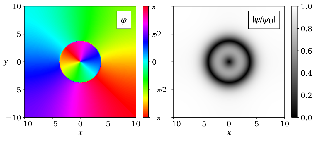
While we have demonstrated a rich spectrum of new solutions in imbalanced systems, the natural question is how they interact with the familiar soliton excitations, namely vortices. We consider a regime away from the LO instability (exemplified by the choice ) where ordinary vortex solutions exist (namely, away from the regime where a vortex core induces an FFLO state as reported in Inotani et al. 2020). We find that the solitons and vortices form bound states, shown in FIG. 5. The energy of this bound state is lower than the combined energy of a separate single vortex and soliton, but the energy of the bound state is larger than the energy of a single ordinary vortex.
VII Solitons in Fulde-Ferrell State: stable vortex-antivortex pairs
Finally, our results prompt the question of whether or not these solitons exist over the background of another imbalanced state with uniform density: namely the Fulde-Ferrell (FF) state, where the background phase modulates. An example of a microscopically derived Ginzburg-Landau model for the FF state can be found in Agterberg and Yang 2001. To model the FF state, without fine-tuning, we chose parameters , , and phenomenologically. Our numerical studies suggested that the solitons described above, are not stable on top of the FF ground state but that the Fulde-Ferrell state has its own stable solitonic excitations of a different kind: vortex-antivortex pairs. In contrast, we did not observe such a solution outside of the FF regime. In FIG. 6 we show a stable vortex-antivortex pair and examples of the structures that can be formed by multiple pairs.

VIII Conclusions
In conclusion, we have shown that in BCS superfluids and superconductors, fermionic imbalance leads to solitonic excitations in the form of ring solitons. These solitons constitute a number of local minima of the free energy landscape. The solutions we find are related to, but distinctly different from, solutions of the Swift-Hohenberg equation. We have shown that these solitons have nontrivial nonlinear bound states: soliton sacks. Additionally, the long-range intersoliton forces predict bound states at larger separation, and the introduction of phase winding generates bound states of solitons with vortices. We have also demonstrated the existence of stable solitonic states in a phase-modulating background, in the form of vortex-antivortex pairs.
In ultracold atoms, ring solitons could be created and observed by imprinting methods and standard density-sensitive techniques, due to the fact that order parameter modulation is typically accompanied by density modulation Samoilenka et al. 2020b; Patton and Sheehy 2020. In a superconductor, such solitons could be observed via scanning tunneling microscopy.
Let us now remark on the particular case of the soliton, that was reported earlier by one of the authors The. Objects structurally similar to the simplest ring soliton have since been discussed independently in the study of unitary Fermi gases at low temperature Magierski et al. 2019; Tüzemen et al. 2020, suggesting that radial solitons may appear under different circumstances from those in the BCS limit. It would be interesting to consider whether unitary systems support more complex bound states, such as soliton sacks, similar to those found in this paper.
Another avenue for further work is to study the dynamics of the presented static solutions. Introducing simple time dependence to the system will lead to dissipative dynamics, equivalent to gradient flow. Since the static solutions we present are local minima of the free-energy landscape, various initial conditions would simply relax to the static solutions presented. However, one interesting question is the behavior of the solitons in a dynamically driven system. A further important question is the height of the energy barrier that prevents the solitons from collapsing. To determine the barrier height quantitatively, techniques such as the string method E et al. 2002; E et al. 2007, recently generalized to superconducting models Benfenati et al. 2020, should be used.
acknowledgments
We thank Andrea Benfenati and Martin Speight for useful discussions. The work was supported by Swedish Research Council Grants No. 642-2013-7837, 2016-06122, and 2018-03659, the Göran Gustafsson Foundation for Research in Natural Sciences and Medicine, Olle Engkvists Stiftelse, and the UK Engineering and Physical Sciences Research Council through Grant No. EP/P024688/1. The computations were performed on resources provided by the Swedish National Infrastructure for Computing (SNIC) at the National Supercomputer Center in Linköping, Sweden, partially funded by the Swedish Research Council through Grant Agreement No. 2018-05973.
Appendix A Rescaling of Ginzburg-Landau functional
In this paper we use the Ginzburg-Landau (GL) free energy expansion derived in Buzdin and Kachkachi 1997, starting from the following microscopic Hamiltonian for a spin-imbalanced superfluid
| (10) | |||
where is the fermionic quantum field operator, is the Zeeman splitting energy, is the superfluid order parameter and H.c. denotes Hermitian conjugation. The resulting GL free energy functional reads
| (11) |
where the coefficients , and are functions of the temperature and the Zeeman splitting energy . In natural units , the coefficients , and are given by
| (12) | ||||
| (13) | ||||
| (14) |
where is the electron density of states at the Fermi surface, is the critical temperature at , and
| (15) |
where and is the polygamma function of order . The remaining coefficients are given in terms of and as , , and , where is the Fermi velocity and , and are positive constants that depend on the dimensionality of the Fermi surface. The numerical values of , and in one, two and three dimensions are given in TABLE 1. The possibility of inhomogeneous ground states arises in the parameter regime in which the gradient coefficient is negative. Since shares sign with the quartic coefficient , the inclusion of positive higher-order terms, both in density and momentum, is necessary.
For convenience we perform the following rescaling
| (16) |
where , , and and the rescaled free energy reads
| (17) |
where denotes the gradient with respect to and and . The values of and in one, two and three dimensions are listed in TABLE 1. In the rescaled coordinates, to be explicit, the length is measured in units of , where
| (18) |
is a dimensionless quantity that diverges as the tricritical point is approached. In the main text, we drop the tilde notation but still work in the rescaled model.
| 1 | 1 | 4 | 4 | 8 | |
| 2 | 2 | ||||
| 3 |
Appendix B Connection to the Swift-Hohenberg equation
The equation of motion corresponding to the Ginzburg-Landau model discussed in the main text reads
| (19) | |||
If we constrain to be real and rescale it by , we obtain the following equation for
| (20) |
where , and . Note, that Eq. (20) becomes the static cubic-quintic Swift-Hohenberg equation, in the limit .
Appendix C Linearization
In this Appendix we will show the technical details as to how the linearized solutions presented in this paper for the long-range behavior of the field were found. From our numerical solutions it follows that there is a class of solutions which can be described by a real field; thus in the analysis below we can restrict the field to be real. The resulting equation of motion reads
| (21) |
where is the potential density. However, as we are interested in the behavior of the soliton far from it’s center, we write the field as,
| (22) |
where we assume that the deviation from the uniform ground state has only radial dependence, is real, and is small. We can then proceed by considering the resulting equation of motion for by neglecting any terms in Eq. (21) that are nonlinear in , as they will be negligible at long range. This results in the linearized equation of motion
| (23) |
Let us define the coefficients
| (24) | ||||
| (25) |
such that the linearized equation of motion reads
| (26) |
which can be written, by introducing , as a system of coupled differential equations
| (27) |
By linear transformation to the eigenbasis of the matrix , the two equations decouple into
| (28) |
where are the two eigenvalues of the matrix . We identify Eq. (28) as the modified Bessel equation, where for each eigenvalue of , the solution in general is given as a superposition of the modified zeroth order Bessel functions and . The Bessel function can be discarded directly by considering the asymptotic behavior at , and we obtain
| (29) |
where are some complex constants, and where we have defined with , which is shown for the relevant parameter regime in FIG. 7. The small deviation is some superposition of and . However, since is real valued, we can use that and consequently , which gives us
| (30) |
where is some complex-valued constant.
Appendix D Long-distance interaction
Next we follow the point-source approach Speight 1997 to determine the intersoliton forces. To that end, let us determine the point source that replicates the asymptotic field given by Eq. (30). The point source is defined by the equation
| (31) |
and can be found by considering the limit , where . Using that , we find
| (32) | ||||
| (33) |
where we have used that for . Inserting these results into Eq. (31) gives the point source
| (34) |
Having calculated the appropriate point source, we now consider two solitons, centered around and , respectively, where the distance is large. To estimate the interaction between the two solitons, we assume that the total field is given by the superposition , where is the deviation from the ground state for one soliton, centered around . That is, approaches far from its center. The main assumption here is that the field of the first soliton at the position of the second is the same as it would have been if there were no soliton there, and vice versa. This is quite a crude approximation since the center contributes significantly to the interaction energy. The interaction energy is derived by expanding to first order in the value of near , and vice versa. After several integrations by parts we can get rid of the exact solitons in favor of their asymptotics , resulting in the interaction energy
| (35) |
By using the derived expression for the asymptotic in Eq. (30) and the point source in Eq. (34) we find
| (36) |
where are the constants associated with the two soliton asymptotics respectively. The oscillatory nature of implies that the solitons will be weakly bound at large distances.
References
- Jackiw and Rebbi (1976) R. Jackiw and C. Rebbi, “Solitons with fermion number ½,” Phys. Rev. D 13, 3398–3409 (1976).
- Heeger et al. (1988) A. J. Heeger, S. Kivelson, J. R. Schrieffer, and W. P. Su, “Solitons in conducting polymers,” Rev. Mod. Phys. 60, 781–850 (1988).
- Goldstone and Wilczek (1981) Jeffrey Goldstone and Frank Wilczek, “Fractional quantum numbers on solitons,” Phys. Rev. Lett. 47, 986–989 (1981).
- Yefsah et al. (2013) Tarik Yefsah, Ariel T. Sommer, Mark J.H. Ku, Lawrence W. Cheuk, Wenjie Ji, Waseem S. Bakr, and Martin W. Zwierlein, “Heavy solitons in a fermionic superfluid,” Nature 499, 426–430 (2013).
- Lutchyn et al. (2011) Roman M. Lutchyn, Maxim Dzero, and Victor M. Yakovenko, “Spectroscopy of the soliton lattice formation in quasi-one-dimensional fermionic superfluids with population imbalance,” Phys. Rev. A 84, 033609 (2011).
- Efimkin and Galitski (2015) Dmitry K. Efimkin and Victor Galitski, “Moving solitons in a one-dimensional fermionic superfluid,” Phys. Rev. A 91, 023616 (2015).
- Ku et al. (2016) Mark J. H. Ku, Biswaroop Mukherjee, Tarik Yefsah, and Martin W. Zwierlein, “Cascade of solitonic excitations in a superfluid fermi gas: From planar solitons to vortex rings and lines,” Phys. Rev. Lett. 116, 045304 (2016).
- Ren and Aleiner (2019) Tianhao Ren and Igor Aleiner, “Solitons in one-dimensional systems at the bcs-bec crossover,” Phys. Rev. A 99, 013626 (2019).
- Dutta and Mueller (2017) Shovan Dutta and Erich J. Mueller, “Collective modes of a soliton train in a fermi superfluid,” Phys. Rev. Lett. 118, 260402 (2017).
- Alford et al. (2001) Mark Alford, Jeffrey A. Bowers, and Krishna Rajagopal, “Crystalline color superconductivity,” Phys. Rev. D 63, 074016 (2001).
- Zwierlein et al. (2006) Martin W. Zwierlein, André Schirotzek, Christian H. Schunck, and Wolfgang Ketterle, “Fermionic superfluidity with imbalanced spin populations,” Science 311, 492–496 (2006).
- Radzihovsky (2011) Leo Radzihovsky, “Fluctuations and phase transitions in larkin-ovchinnikov liquid-crystal states of a population-imbalanced resonant fermi gas,” Phys. Rev. A 84, 023611 (2011).
- Samoilenka et al. (2020a) Albert Samoilenka, Filipp N. Rybakov, and Egor Babaev, “Synthetic nuclear skyrme matter in imbalanced fermi superfluids with a multicomponent order parameter,” Phys. Rev. A 101, 013614 (2020a).
- Bulgac and Forbes (2008) Aurel Bulgac and Michael McNeil Forbes, “Unitary fermi supersolid: The larkin-ovchinnikov phase,” Phys. Rev. Lett. 101, 215301 (2008).
- Radzihovsky and Sheehy (2010) Leo Radzihovsky and Daniel E Sheehy, “Imbalanced feshbach-resonant fermi gases,” Reports on Progress in Physics 73, 076501 (2010).
- Son and Stephanov (2006) D. T. Son and M. A. Stephanov, “Phase diagram of a cold polarized fermi gas,” Phys. Rev. A 74, 013614 (2006).
- Bianchi et al. (2003) A. Bianchi, R. Movshovich, C. Capan, P. G. Pagliuso, and J. L. Sarrao, “Possible fulde-ferrell-larkin-ovchinnikov superconducting state in ,” Phys. Rev. Lett. 91, 187004 (2003).
- Cho et al. (2017) Chang-woo Cho, Jonathan Haiwei Yang, Noah F. Q. Yuan, Junying Shen, Thomas Wolf, and Rolf Lortz, “Thermodynamic evidence for the fulde-ferrell-larkin-ovchinnikov state in the superconductor,” Phys. Rev. Lett. 119, 217002 (2017).
- Uji et al. (2018) S. Uji, Y. Iida, S. Sugiura, T. Isono, K. Sugii, N. Kikugawa, T. Terashima, S. Yasuzuka, H. Akutsu, Y. Nakazawa, D. Graf, and P. Day, “Fulde-ferrell-larkin-ovchinnikov superconductivity in the layered organic superconductor ,” Phys. Rev. B 97, 144505 (2018).
- Mayaffre et al. (2014) H. Mayaffre, S. Krämer, M. Horvatić, C. Berthier, K. Miyagawa, K. Kanoda, and V. F. Mitrović, “Evidence of Andreev bound states as a hallmark of the FFLO phase in -(BEDT-TTF)2CuNCS)2,” Nature Physics 10, 928–932 (2014).
- Coniglio et al. (2011) William A. Coniglio, Laurel E. Winter, Kyuil Cho, C. C. Agosta, B. Fravel, and L. K. Montgomery, “Superconducting phase diagram and fflo signature in -(bets)2gacl4 from rf penetration depth measurements,” Phys. Rev. B 83, 224507 (2011).
- Norman (1993) M. R. Norman, “Existence of the fflo state in superconducting ,” Phys. Rev. Lett. 71, 3391–3391 (1993).
- Cho et al. (2011) K. Cho, H. Kim, M. A. Tanatar, Y. J. Song, Y. S. Kwon, W. A. Coniglio, C. C. Agosta, A. Gurevich, and R. Prozorov, “Anisotropic upper critical field and possible fulde-ferrel-larkin-ovchinnikov state in the stoichiometric pnictide superconductor lifeas,” Phys. Rev. B 83, 060502 (2011).
- Matsuda and Shimahara (2007) Yuji Matsuda and Hiroshi Shimahara, “Fulde-ferrell-larkin-ovchinnikov state in heavy fermion superconductors,” Journal of the Physical Society of Japan 76, 051005 (2007).
- Lortz et al. (2007) R. Lortz, Y. Wang, A. Demuer, P. H. M. Böttger, B. Bergk, G. Zwicknagl, Y. Nakazawa, and J. Wosnitza, “Calorimetric evidence for a fulde-ferrell-larkin-ovchinnikov superconducting state in the layered organic superconductor ,” Phys. Rev. Lett. 99, 187002 (2007).
- Singleton et al. (2000) J Singleton, J A Symington, M-S Nam, A Ardavan, M Kurmoo, and P Day, “Observation of the fulde-ferrell-larkin-ovchinnikov state in the quasi-two-dimensional organic superconductor -(BEDT-TTF)2cu(NCS)2(BEDT-TTF=bis(ethylene-dithio)tetrathiafulvalene),” Journal of Physics: Condensed Matter 12, L641–L648 (2000).
- Martin et al. (2005) C. Martin, C. C. Agosta, S. W. Tozer, H. A. Radovan, E. C. Palm, T. P. Murphy, and J. L. Sarrao, “Evidence for the fulde-ferrell-larkin-ovchinnikov state in from penetration depth measurements,” Phys. Rev. B 71, 020503 (2005).
- Agterberg et al. (2014) Daniel F. Agterberg, Egor Babaev, and Julien Garaud, “Microscopic prediction of skyrmion lattice state in clean interface superconductors,” Phys. Rev. B 90, 064509 (2014).
- Barkman et al. (2019a) Mats Barkman, Alexander A. Zyuzin, and Egor Babaev, “Antichiral and nematicity-wave superconductivity,” Phys. Rev. B 99, 220508 (2019a).
- Fulde and Ferrell (1964) P. Fulde and R. A. Ferrell, “Superconductivity in a Strong Spin-Exchange Field,” Physical Review 135, 550–563 (1964).
- Larkin and Ovchinnikov (1964) A. I. Larkin and Y. N. Ovchinnikov, “Nonuniform state of superconductors,” Zh. Eksp. Teor. Fiz. 47, 1136–1146 (1964), [Sov. Phys. JETP20,762(1965)].
- (32) Preliminary results, demonstrating existence of the ring solitons in imbalanced systems were presented in the Master thesis work: M. Barkman, Investigation of Order Parameter Structures of the Fulde-Ferrell-Larkin-Ovchinnikov State in Superconductors Using the Finite Element Method, M.S. thesis, KTH School of Engineering Sciences, 2018, https://www.diva-portal.org/smash/get/diva2:1241674/FULLTEXT01.pdf.
- Buzdin and Kachkachi (1997) A.I. Buzdin and H. Kachkachi, “Generalized ginzburg-landau theory for nonuniform fflo superconductors,” Physics Letters A 225, 341 – 348 (1997).
- Agterberg and Yang (2001) D F Agterberg and Kun Yang, “The effect of impurities on fulde-ferrell-larkin-ovchinnikov superconductors,” Journal of Physics: Condensed Matter 13, 9259–9270 (2001).
- Barkman et al. (2019b) Mats Barkman, Albert Samoilenka, and Egor Babaev, “Surface pair-density-wave superconducting and superfluid states,” Phys. Rev. Lett. 122, 165302 (2019b).
- Samoilenka et al. (2020b) Albert Samoilenka, Mats Barkman, Andrea Benfenati, and Egor Babaev, “Pair-density-wave superconductivity of faces, edges, and vertices in systems with imbalanced fermions,” Phys. Rev. B 101, 054506 (2020b).
- Swift and Hohenberg (1977) J. Swift and P. C. Hohenberg, “Hydrodynamic fluctuations at the convective instability,” Phys. Rev. A 15, 319–328 (1977).
- Hecht (2012) F. Hecht, “New development in freefem++,” J. Numer. Math. 20, 251–265 (2012).
- Speight et al. (2019) Martin Speight, Thomas Winyard, and Egor Babaev, “Chiral -wave superconductors have complex coherence and magnetic field penetration lengths,” Phys. Rev. B 100, 174514 (2019).
- Speight (1997) J. M. Speight, “Static intervortex forces,” Phys. Rev. D 55, 3830–3835 (1997).
- Sakaguchi and Brand (1996) Hidetsugu Sakaguchi and Helmut R. Brand, “Stable localized solutions of arbitrary length for the quintic swift-hohenberg equation,” Physica D: Nonlinear Phenomena 97, 274 – 285 (1996).
- Lloyd and Sandstede (2009) David Lloyd and Björn Sandstede, “Localized radial solutions of the swift–hohenberg equation,” Nonlinearity 22, 485–524 (2009).
- Garaud et al. (2011) Julien Garaud, Johan Carlström, and Egor Babaev, “Topological solitons in three-band superconductors with broken time reversal symmetry,” Phys. Rev. Lett. 107, 197001 (2011).
- Garaud et al. (2013) Julien Garaud, Johan Carlström, Egor Babaev, and Martin Speight, “Chiral skyrmions in three-band superconductors,” Phys. Rev. B 87, 014507 (2013).
- Rybakov and Kiselev (2019) Filipp N. Rybakov and Nikolai S. Kiselev, “Chiral magnetic skyrmions with arbitrary topological charge,” Phys. Rev. B 99, 064437 (2019).
- Foster et al. (2019) David Foster, Charles Kind, Paul J Ackerman, Jung-Shen B Tai, Mark R Dennis, and Ivan I Smalyukh, “Two-dimensional skyrmion bags in liquid crystals and ferromagnets,” Nature Physics 15, 655–659 (2019).
- Inotani et al. (2020) Daisuke Inotani, Shigehiro Yasui, Takeshi Mizushima, and Muneto Nitta, “Radial fulde-ferrell-larkin-ovchinnikov state in a population-imbalanced fermi gas,” (2020), arXiv:2003.03159 [cond-mat.quant-gas] .
- Patton and Sheehy (2020) Kelly R. Patton and Daniel E. Sheehy, “Hartree-fock-bogoliubov theory of trapped one-dimensional imbalanced fermi systems,” Phys. Rev. A 101, 063607 (2020).
- Magierski et al. (2019) Piotr Magierski, Buğra Tüzemen, and Gabriel Wlazłowski, “Spin-polarized droplets in the unitary fermi gas,” Phys. Rev. A 100, 033613 (2019).
- Tüzemen et al. (2020) B. Tüzemen, P. Kukliński, P. Magierski, and G. Wlazłowski, “Properties of spin-polarized impurities - ferrons, in the unitary fermi gas,” Acta Phys. Pol. B 51, 595 (2020).
- E et al. (2002) Weinan E, Weiqing Ren, and Eric Vanden-Eijnden, “String method for the study of rare events,” Phys. Rev. B 66, 052301 (2002).
- E et al. (2007) Weinan E, Weiqing Ren, and Eric Vanden-Eijnden, “Simplified and improved string method for computing the minimum energy paths in barrier-crossing events,” The Journal of Chemical Physics 126, 164103 (2007).
- Benfenati et al. (2020) Andrea Benfenati, Andrea Maiani, Filipp N. Rybakov, and Egor Babaev, “Vortex nucleation barrier in superconductors beyond the bean-livingston approximation: A numerical approach for the sphaleron problem in a gauge theory,” Phys. Rev. B 101, 220505 (2020).