Interaction driven polarization shift in the lattice fermion model at half filling: emergent Haldane phasePreprint: APS/123-QED
Abstract
We study the model in one dimension at half-filling. It is known that for large enough fixed, as is varied, the system goes from a charge-density wave into a Luttinger liquid, then a bond-order, and then a second charge density wave phase. We find that the Luttinger liquid state is further split into two, separating parts with distinct values of the many-body polarization Berry phase. Inside this phase, the variance of the polarization is infinite in the thermodynamic limit, meaning that even if the polarization differs, it would not be measurable. However, in the gapped phases on each side of the Luttinger liquid, the polarization takes a different measurable value, implying topologically distinction. The key difference is that the large- phases are link-inversion symmetric, while the small- one is site-inversion symmetric. We show that large- phase can be related to an spin chain, and exhibits many features of the Haldane phase. The lowest lying states of the entanglement spectrum display different degeneracies in the two cases, and we also find string order in the large- phase. We also study the system under open boundary conditions, and suggest that the number of defects is related to the topology.
I Introduction
Topological condensed matter systems constitute an active research area. Topological band insulators are well understood. Bernevig13; Asboth16; Franz13 Quantum phase transitions occur when the relevant topological invariant ( or ) undergoes a finite change at a gap closure point. These systems also obey the bulk-boundary correspondence principle (BBCP), which predicts the existence of edge states in the topologically non-trivial phases.
Recently, attention has focused Franz13; Raghu08; Fidkowski10; Pollmann10; Fidkowski11; Turner11; Pollmann12; Manmana12; Yoshida14; Rachel18 on interacting systems. An early result is the Haldane conjecture, Haldane83a; Haldane83b; Affleck89 which is based on a field-theoretical mapping of the Heisenberg model to a continuum one, and states that spin chains are topologically non-trivial and exhibit spin- edge states. A useful scheme to visualize this state of affairs is the Affleck, Kennedy, Lieb, and Tasaki (AKLT) wave function, also known as the valence bond solid (VBS), a model for systems. Recently Oshikawa Oshikawa92 extended the AKLT wave function to arbitrary integer spin models. Pollmann et al. Pollmann12 showed that topological protection is present only in odd- systems, and the protecting symmetries are time-reversal, dihedral rotation, and link inversion.


The generalization of the idea of a topological invariant to the many-body case is also a crucial question, since topological invariants Bernevig13; Asboth16; Franz13 in non-interacting systems are integrals over Bloch states. Manmana et al. Manmana12 define an invariant using the single particle Green’s function and the chiral symmetry operator. The invariant obtained this way reduces to the known invariant if the system is non-interacting. In the interacting case, topological edge states can arise in three ways: poles or zeros in the Green’s function (single-particle effects) or spontaneous symmetry breaking at the edge (many-body effect). The latter is not necessarily picked up by a topological invariant defined based on the single-particle Green’s function. The polarization Berry phase Resta98; Resta99 reduces to the Zak phase when a non-interacting system is considered, however, in the interacting case it is a genuine many-body expectation value.
In this paper we study the one-dimensional interacting lattice model of spinless fermions. denotes the hopping parameter, the nearest neighbor interaction, and the next nearest neighbor interaction. It is known Mishra11 that at large enough a scan in will find four phases: charge density wave (CDW-1), Luttinger liquid (LL), bond-order (BO), and a different charge density wave (CDW-2) phase. Our central finding is that at a critical the LL phase is split into two parts. For the Berry phase is zero, for it is . In the LL phase, in the thermodynamic limit, the variance of the polarization diverges with system size, thus the different polarization averages are not measurable (expected for a gapless phase). However, on the different sides of the LL phase, the phases are such that the polarizations are measurable, and the discrete difference between the two implies Watanabe18 topological distinction. In particular we find that the CDW-2 exhibits parallels to a Haldane phase. Haldane83a; Haldane83b We show this via a mapping of our original Hamiltonian to an spin model, by calculating the entanglement spectrum, and by showing that hidden antiferromagnetic (HAFM) order as well as finite range string correlation, as defined by den Nijs and Rommelse denNijs89 is present. We also analyze the system with open boundary conditions: our results here suggest that the number of defects in a particular ordered phase may be connected to the value of the topological invariant.
The paper is organized as follows. In section II the model is presented, as well as its connection to integer- quantum spin chains. In section III the polarization amplitude is introduced. It is shown that link inversion gives rise to a non-trivial Berry phase, and several variants of the Lieb-Schultz-Mattis Lieb61 (LSM) theorem pertinent to our study are derived. In section IV our numerical results are presented, in section V we conclude our work.

II Model Hamiltonian
The model already has a long history. Hallberg90; Zhuravlev97; Poilblanc97; Mishra11 While evidence for the four different phases was known since the early study, Hallberg90 the precise phase diagram was only established recently by Mishra et al. Mishra11 The Hamiltonian of the model is
| (1) |
We take as the energy scale. The Hamiltonian can be mapped Hallberg90 onto a spin- chain, via a Jordan-Wigner transformation,
| (2) |
It is obvious that dihedral -rotation symmetry is a symmetry of the Hamiltonian. Rotation of each spin by around a chosen axis, , , or returns to itself. Time reversal and link inversion are also symmetries of . In Ref. Pollmann12 these three symmetries were found to be the ones protecting the topological Haldane phase in odd- spin chains.
The canonical example of the topological Haldane phase is the Heisenberg model. Crucial insight into the behavior of this model can be gained via the AKLT variational state whose elementary components are sites, but it is constructed in such a way that pairs of AKLT sites correspond to a true site of the system. This construction is also mentioned in Manmana et al. Manmana12 to relate one-dimensional fermion models (or models) to spin models in the example they use, which is an SSH type model Su79 with a Hubbard interaction.
We can proceed in an analogous manner in the model. We divide the Hamiltonian in Eq. (2) into two pieces:
| (3) | |||||
Note that consists of uncoupled pairs of sites. As in the AKLT procedure, we express in an (truncated) basis , and . In this basis becomes an onsite term,
| (4) |
turns out to be a pairing term of the form:
| (5) |
The Hamiltonian was studied Oshikawa92 in detail in the context of the Haldane phase. The symmetries which protect Pollmann12 the Haldane phase in odd- systems, namely, time-reversal, dihedral rotation, and link inversion, are all present in this Hamiltonian, and HAFM and string order denNijs89 are also exhibited. While this Hamiltonian is a mapping based on a truncated basis (the states are missing), below we show that this is not relevant, a Haldane phase is still exhibited, since the additional terms account for states of .
In addition to exact diagonalization of the Hamiltonian (Eq. (1)), we also perform auxiliary calculations. We construct a variational wave function, which can be viewed as the marriage of the AKLT wave function with the Baeriswyl variational wave function. Baeriswyl86; Baeriswyl00 In the AKLT scheme an site is considered as two spin sites. Bonds connecting different -sites are taken to be in singlet states. A projector is applied to the -sites themselves, projecting them into states.
In our case, we start with an ordered state for , a state with alternating pairs of occupied and unoccupied sites, , and apply the projector
| (6) |
where is the Hamiltonian without the second-nearest neighbor coupling term, but including the hopping energy and the nearest neighbor coupling term. is a variational parameter. The projector is only applied between bonds connecting an occupied and an unoccupied site ( or ). The wave function is represented in tensor network notation of Ref. Orus14 in the lower panel of Fig. 3, where a comparison the energies of this scheme compared to exact diagonalization results is also shown. The results indicate that this wave function provides an accurate description of the system.
In our study of the system with open boundary conditions, we also complement our exact diagonalization results with a cluster mean-field theory calculation. Here clusters of four sites are solved exactly, but the inter-cluster couplings are considered at the mean-field level. We do this for the case of open boundary conditions, meaning that the mean-field parameters for each cluster vary as a function of the position of the cluster in the lattice.

III Polarization amplitude, symmetry analysis, and topological analogy
Topological invariants for non-interacting systems Thouless82; Kane05a; Kane05b; Fu06 are quantities derived from geometric phases Berry84; Zak89 (Zak phase). The Zak phase, the topological invariant sensitive to the transition King-Smith93; Resta94 in the SSH model, Su79 has a straightforward many-body generalization Resta98; Resta99 (a single-point Berry phase Resta00). We define the polarization amplitude,
| (7) | |||||
where . The operator is known as the total momentum shift operator. In terms of the polarization Resta98; Aligia99 of a system with filling per unit cell can be written as
| (8) |
This expression can be shown Resta98; King-Smith93 to be consistent with the modern theory of polarization. The variance Resta99 of the total position as well as higher order cumulants Souza00 can also be derived Hetenyi19, under the assumption that is the analog of a characteristic function, defined on a discrete set of points ( take only integer values). The polarization of Resta Resta98 is the first moment of this characteristic function, while the variance of Resta and Sorella Resta99 is the second cumulant. Both can be obtained Hetenyi19 via finite difference derivatives with respect to . Recently, was intensively studied Aligia99; Nakamura02; Yahyavi17; Kobayashi18; Hetenyi19; Nakamura19; Furuya19 as a source of information about quantum phase transitions and the associated finite size scaling. In this work, exploiting the fact that is a characteristic function, we analyze its Fourier transform,
| (9) |
understood to be the polarization distribution of the system, defined over the lattice positions . The summation index runs over all components of the polarization amplitude . The Aligia and Ortiz Aligia99 correction is automatically considered. For example, if a system has half filling, , then there will be no odd- contributions, and will have two peaks within one supercell (see Figs. 1 and 2).
Due to half-filling, all for odd are zero. In the limiting cases and the nonzero take the following values Hetenyi19: while for the former, and alternates between for the latter. We can also generally demonstrate the role of link inversion symmetry by generalizing a result of Zak Zak89 to the many-body case. In Zak’s original paper Zak89 it was argued that the Zak phase takes a trivial value (zero) in the case of inversion symmetry about a lattice site, while a non-trivial value is taken if the inversion symmetry is about the bond-center () (also known as link-inversion symmetry). Zak showed this by first expressing the Zak phase,
| (10) |
using Wannier functions as
| (11) |
In Eqs. (10) and (11) denotes the size of the unit cell and is the Wannier function for some band. If the system obeys reflection symmetry about a lattice site, then , leading to (equivalent to shifts by ). For the case of link inversion symmetry, , leads to .
Our task is to generalize this argument to the many body case. Our starting point is the phase of the many-body polarization expression derived by Resta, Resta98; Resta99 applied to a half-filled system Aligia99 (filling , where ),
| (12) |
We apply a site-centered reflection to the total momentum shift operator,
| (13) |
In this case the site around which reflection was performed was chosen to be the one at the origin. It is easily seen that . We now apply a reflection operator around a bond center, using
| (14) |
leads to the result: . This result was also shown for matrix product states which are not “cat states” (superposition of two states not connected by any local operator) in Ref. Pollmann12. Our proof above is entirely general.
In addition to the above result, we can also prove a version of the
LSM theorem relevant to our model. The original LSM theorem shows
that spin-chains behave qualitatively different, depending on the spin
being integer or half-integer. In our case, the distinction depends
on whether a model exhibits site or link-inversion symmetry.

We start with a ground state of a model whose Hamiltonian consists of a hopping of the type in Eq. (1), and some coordinate dependent interaction term. We construct a new state
| (15) |
The energy of this state compared to the ground state is
| (16) |
In the thermodynamic limit, the , but may not be a state that is different from . To show this, apply the different inversion operators () and time reversal symmetry, as
| (17) | |||||
The state is even if the system is site-inversion
symmetric, while odd in the case of bond-inversion symmetry. The two
possibilities arising from these results are the following. In the
thermodynamic limit, there may be a gapless excitation which is odd
with respect to bond inversion, alternatively, bond inversion symmetry
may be spontaneously broken with degenerate ground states with a gap
above each.

One model analyzed by Manmana et al. Manmana12 was a spinful SSH model Su79 with a Hubbard interaction. We show here, that the results derived above for the model hold for the spinful SSH model as well. Let us write it in the following form:
| (18) |
() are creation operators on the different sublattices. In order to prove either of the above results, it is sufficient to consider one spin channel, and define a momentum shift operator of the form
| (19) |
One can use this operator to construct a state , and the energy difference will be
| (20) |
Eq. (17) holds meaning that a bond-inversion symmetric
system will have a degenerate ground state.
The basis used to construct and is a truncated one, the state is missing. Still, we can formulate a theorem of the Lieb-Schultz-Mattis type, as was done above. The relevant operator is
| (21) |
If one applies the steps above to a fixed spin model (applying link-inversion, and time reversal), the result is a sign change in for an odd- model, but no sign change for an even- model. This is consistent with the results of Ref. Pollmann12. The fact that the basis is a truncated one for our case makes no difference, since other states are states, and the maximum spin a site can be is .
IV Exact diagonalization results
The results of Mishra et al. Mishra11 for the phase diagram are shown in Fig. 1, upper panel. The phase lines separate a charge-density wave (CDW-1) a LL, a bond-order and a second charge-density (CDW-2) wave phase. Our main result is that in addition to the known Mishra11 phase diagram, we find the dashed line inside the LL phase which separates phases in which the polarization (average of the polarization distribution) differs by one-quarter of a supercell (see Fig. 1 lower panel). Along the transition line the polarization distribution, is flat. Moving away in either direction gives distributions with maxima in different places. Since the filling with respect to number of unit cells is , corresponds to the polarization. Aligia99 The inset of the upper panel of Fig. 1 shows the reconstructed distribution for selected points along the line with different values of below, at and above the transition point (points are indicated in the main figure with asterisks, upper panel). The transition in this case occurs at , where is entirely flat. The positions of the two maxima both shift at the transition point.

Fig. 2 shows the distributions for different system sizes for four cases. The distributions are scaled by the system size on the -axis to enable comparison. Two cases which are in the LL phase are shown (), as well as two other cases in the two different CDW phases (, and ). The CDW distributions show sharp peaks, whereas in the LL phase the distributions have smeared out maxima. We also calculated the size scaling exponent of the variance of the polarization, shown in the lower right inset of the upper panel of Fig. 1. The variance was calculated according to the procedure in Ref. Hetenyi19. The size scaling exponent was calculated by fitting the variance as a function of system size to the function . Clearly, the two LL phases exhibit , meaning that the variance of the polarization scales as the square of the system size for both cases. This also means that the polarization distributions in the phase flatten as . They behave in a similar manner to the phase transition line within the LL phase shown in Fig. 1. Even though finite systems exhibit a fixed average polarization, since the variance diverges with system size, it will not be an experimentally measurable quantity. In contrast, both insulating phases show a near one.
The following picture emerges. The gapless LL phase, in which the polarization distribution is flat in the limit of large system size, separates gapped phases in which the polarizations differ by a quarter of a lattice constant. This corresponds to a shift in Zak phase of , exactly as in the case of the SSH model. However, unlike in that model, the topologically distinct phases are not separated by one phase transition point. Instead, they are separated by the entire LL phase. In the finite system, the LL phase exhibits a topological phase line, on either side of which the polarization distribution is distributed according to a Gaussian whose variance diverges with system size. In the insulating phases on either side, the distributions are peaked and have finite variances, even in the thermodynamic limit, the polarization therefore is measurable.
The upper panel of Fig. 3 shows two graphs low lying states of the entanglement spectrum for a system with as a function of for two different entanglement cuts. The system consists of sites with periodic boundary conditions. In one case (uppermost graph) the entanglement cut is taken at half the system ( and the environment is which is traced out), while in the middle panel, the entanglement cut is taken such that the subsystem size is , the environment (traced out) is sites. In both graphs, the lowest lying state is two-fold degenerate in the CDW-1 phase, while it is four-fold degenerate in the CDW-2 phase. In the case the two states in the CDW-1 phase form a basis for a two dimensional irreducible representation of the link inversion operator. The four states in the CDW-2 phase form a basis for two two dimensional irreducible representations of the link inversion operator. For the case the two degenerate states on the CDW-1 side form two identity representations of the site-inversion operator, while on the CDW-2 side, we find, again, two two-dimensional representations thereof.
We also calculated the entanglement spectrum (for a system with and an entanglement cut at half the system) for the variational ansatz shown in Fig. 3. Since the symmetry is explicitly broken in this variational wave function, there are four different ways to choose such an entanglement cut. Each different cut gives rise to one low-lying state in the entanglement spectrum, consistent with the fourfold degneracy of the CDW-2 phase found via exact diagonalization.
In Fig. 4 we show quantities related to HAFM ordering. By hidden antiferromagnetic (AFM) order we mean Oshikawa92 the following. Once sites are paired, as was done to construct the truncated Hamiltonian in section II, the -component of the spin of the paired sites are calculated (if both sites are occupied, , if one site of the two is occupied, , if both sites are empty, ). In hidden AFM order and sites must alternate, possibly with sites in between. An example of such a configuration is (a configuration in the space of paired sites). In the upper panel of Fig. 4 the fraction of configurations not consistent with hidden AFM order are shown. We see that in the CDW-1 and CDW-2 states, the overwhelming majority of configurations are consistent with hidden AFM. It is only in the ungapped region (mainly the LL phase) where configurations not consistent with hidden AFM are found.
The lower panel of Fig. 4 shows the string order correlation function of den Nijs and Rommelse denNijs89, which is of the form
| (22) |
The CDW-1 state displays a rapidly decaying correlation function, while the CDW-2 state show ordering. For the former, definite conclusions are difficult to draw, due to the small system size, but it appears that there is a decay in the string correlation function.
Manmana et al. Manmana12 analyzed the BBCP in an interacting topological system, a spin-dependent SSH model with Hubbard on-site interaction. This model is presented as an example for symmetry breaking at the edges, as opposed to single-particle topological edge states corresponding to poles or zeros of the single-particle Greens’s function. Symmetry breaking at the edges is a many-body phenomenon to which the single-particle Green’s function based topological invariant is not necessarily sensitive.
Their analysis is not directly applicable to our model due to the finite range of the interactions. We are not able to take a dimerized limit. We can, however, investigate a system with open boundary conditions. The density distribution for our interacting system with open boundary conditions is shown for four cases in Fig. 5 under open boundary conditions. The upper two plots show a CDW-1 () and CDW-2 () examples, while the bottom two show nearly completely ordered CDW-1 and CDW-2 cases. The completely ordered states are interesting because each one is adiabatically connected to all states on the same side of the LL region. All distributions in Fig. 5 invert around the midpoint, meaning that the left edge can be related to the right edge via link inversion symmetry. In Fig. 6 the density distributions are shown for the nearly completely ordered CDW-1 and CDW-2 states based on a four-site cluster mean-field calculation with open boundary conditions. In each case one particular symmetry broken state exists at each edge. In the middle the system has to “connect” between the different symmetry broken states at the edges. For the CDW-1 case one (or an odd number) of defect(s) is needed, while in the CDW-2 case two (or an even number of) defect(s) are required. The defects are indicated by the arrows on the figure.
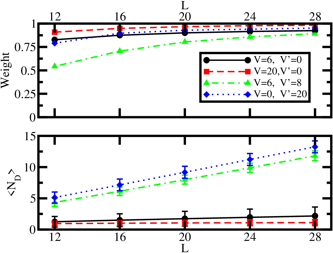
Defects can be located anywhere on the lattice, and the quantum ground state can be a superposition of states with different numbers of defects in different places. Fig. 7 shows the weight of configurations with an odd(even) number of defects for the CDW-1(CDW-2) cases in the ground state wave function. In these calculations, the ground state wave function was obtained in real space. In each real-space component the defects were counted as follows. In the CDW-1 case, there are two ordered states, or , where represents an empty site, , an occupied one. If the left most site is filled, we assume that segment of the system is in the former, if not, then the latter. We then check, starting from the leftmost site, going right, whether the configuration deviates from this ordered state. For example, if the configuration is , the fifth site exhibits a defect. After a defect is encountered, we reset the ordered state accordingly, and look for the next defect. We use a similar scheme for the CDW-2 state, except there, the possible ordered states are , , , and . This means that the first two sites determine an ordered state. When a defect is encountered the resetting to a new ordered state is based on the defect site, and the one before it. The defects counted are of the types indicated in Fig. 6. As the system size increases, the weight of configurations with odd(even) number of defects approaches unity in the CDW-1(CDW-2) ground state. The lower panel of Fig. 7 shows the average number of defects and its variance for the four cases. The number of defects increases linearly with system size.
As mentioned above, it is difficult to construct a model in this case, which identifies the edge state. In the example of Manmana et al. Manmana12 the model was one in which dimerization was possible, and in this limit, the analysis is not much more difficult than for the non-interacting SSH model. In our case, for the CDW-2, such a limit does not exist, however, we can make conjectures based on the results above. It appears that symmetry breaking occurs at the edges, and in order to connect the two boundaries, an odd number of defects is necessary in the CDW-1 phase, and the number of defects needs to be even in the CDW-2 phase. This may be a common scenario in ordinary symmetry broken systems, but most importantly, it coincides with the findings of Manmana et al. Manmana12 In the case of symmetry breaking at the edges in an topological interacting system, a localized edge state may not be easily identifiable, since it is a many-body state, not a single-particle one.
V Conclusion
The main criterion for topological insulation is the topological invariant assuming non-trivial values. In non-interacting systems the invariant undergoes a finite change at a gap closure point. Topologically distinct phases are separated by gap closure points, or quantum phase transitions.
In the model, for fixed large enough to start in a charge-density wave phase, as is increased a Luttinger liquid phase is encountered. Passing through this phase, there is a bond order phase followed by a new charge density wave. The many-body polarization single-point Berry phase changes discontinuously inside the Luttinger liquid phase at a critical . However, in contrast to non-interacting systems, this change in the topological invariant occurs inside a gapless phase. Inside the gapless Luttinger liquid phase the variance of the polarization diverges with system size, meaning that the Berry phase is undefined inside this whole region. In short, topologically distinct phases are separated, not by a quantum phase transition point, as in non-interacting systems, but by the Luttinger liquid phase itself. The topological phase was shown to be a Haldane phase, exhibiting hidden anti-ferromagnetic order and finite string correlation.
The model we studied can be realized experimentally in a cold atoms in optical lattice setting. Bloch08 The degree of control in such experiment places strongly correlated one-dimensional models within reach. Cazalilla11 Particularly pertinent to our study is that the geometric phase Berry84; Zak89 which gauges the transition can also be directly Atala13 measured.
Acknowledgments
This research was supported by the National Research, Development and Innovation Fund of Hungary within the Quantum Technology National Excellence Program (Project Nr. 2017-1.2.1-NKP-2017-00001).
References
- (1) B. A. Bernevig and T. Hughes, Topological Insulators and Topological Superconductors Princeton University Press, (2013).
- (2) J. K. Asbóth, L. Oroszlány, and A. Pályi A Short Course on Topological Insulators Springer (2016).
- (3) M. Franz and L. Molenkamp, Topological Insulators, Contemporary Concepts of Condensed Matter Science, vol. 6, Eds. E. Burstein, A. H. MacDonald, and P. J. Stiles, Elsevier Press, (2013).
- (4) S. Raghu, X.-L. Qi, C. Honerkamp, S.-C. Zhang, Phys. Rev. Lett. 100 156401 (2008).
- (5) L. Fidkowski and A. Kitaev, Phys. Rev. B 81 134509 (2010).
- (6) F. Pollmann, A. M. Turner, E. Berg, M. Oshikawa, Phys. Rev. B 81 064439 (2010).
- (7) L. Fidkowski and A. Kitaev, Phys. Rev. B 83 075103 (2011).
- (8) A. M. Turner, F. Pollmann, and E. Berg, Phys. Rev. B 83 075102 (2011).
- (9) F. Pollmann, E. Berg, A. M. Turner, M. Oshikawa, Phys. Rev. B 85 075125 (2012).
- (10) S. R. Manmana, A. M. Essin, R. M. Noack, and V. Gurarie, Phys. Rev. B 86 205119 (2012).
- (11) T. Yoshida, R. Peters, S. Fujimoto, and N. Kawakami, Phys. Rev. Lett. 112 196404 (2014).
- (12) S. Rachel, Rep. Prog. Phys. 81 116501 (2018).
- (13) F. D. M. Haldane, Phys. Lett. 93A, 464 (1983).
- (14) F. D. M. Haldane, Phys. Rev. Lett. 50, 1153 (1983).
- (15) I. Affleck, J. Phys. Cond. Mat. 1, 3047 (1989).
- (16) M. Oshikawa, J. Phys. Cond. Mat. 4, 7469 (1992).
- (17) H. Watanabe and M. Oshikawa, Phys. Rev. X 8, 021065 (2018).
- (18) R. Resta, Phys. Rev. Lett. 80 1800 (1998).
- (19) R. Resta and S. Sorella, Phys. Rev. Lett. 82 370 (1999).
- (20) T. Mishra, J. Carrasquilla, M. Rigol, Phys. Rev. B 84 115135 (2011).
- (21) M. den Nijs and K. Rommelse, Phys. Rev. B 40 4709 (1989).
- (22) E. Lieb, T. Schultz, and D. Mattis, Ann. Phys. 16 407 (1961).
- (23) K. Hallberg, E. Gagliano, and C. Balseiro, Phys. Rev. B 41 9474 (1990).
- (24) A. K. Zhuravlev, M. I. Katsnelson, and A. V. Trefilov, Phys. Rev. B 56 12939 (1997).
- (25) D. Poilblanc, and S. Yunoki, S. Maekawa, and E. Dagotto, Phys. Rev. B 56 R1645 (1997).
- (26) W. P. Su, J. R. Schrieffer and A. J. Heeger, Phys. Rev. Lett. 42 1698 (1979).
- (27) D. Baeriswyl in Nonlinearity in Condensed Matter, Ed. A. R. Bishop, D. K. Campbell, D. Kumar, and S. E. Trullinger, Springer-Verlag (1986).
- (28) D. Baeriswyl, Found. Physics, 30 2033 (2000).
- (29) R. Orús, Ann. Phys. 349 117 (2014).
- (30) C. L. Kane, and E. J. Mele, Phys. Rev. Lett. 95 146802 (2005).
- (31) C. L. Kane, and E. J. Mele, Phys. Rev. Lett. 95 226801 (2005).
- (32) D. J. Thouless, M. Kohmoto, M. P. Nightingale, M. den Nijs, Phys. Rev. Lett. 49 405 (1982).
- (33) L. Fu and C. L. Kane, Phys. Rev. B 74 195312 (2006).
- (34) M. V. Berry, Proc. Roy. Soc. London A392 45 (1984).
- (35) J. Zak, Phys. Rev. 62 2747 (1989).
- (36) R. D. King-Smith and D. Vanderbilt, Phys. Rev. B 47 1651 (1993).
- (37) R. Resta, Rev. Mod. Phys. 66 899 (1994).
- (38) R. Resta, J. Phys. Cond. Mat. 12 R107 (2000).
- (39) A. A. Aligia and G. Ortiz, Phys. Rev. Lett. 82 2560 (1999).
- (40) I. Souza, T. Wilkens, and R. M. Martin, Phys. Rev. B 62 1666 (2000).
- (41) B. Hetényi and B. Dóra, Phys. Rev. B 99 085126 (2019).
- (42) M. Nakamura and J. Voit, Phys. Rev. B 65 153110 (2002).
- (43) M. Nakamura and S. C. Furuya, Phys. Rev. B 99 075128 (2019).
- (44) S. C. Furuya and M. Nakamura, Phys. Rev. B 99 144426 (2019).
- (45) R. Kobayashi, Y. O. Nakagawa, Y. Fukusumi, M. Oshikawa, Phys. Rev. B 97 165133 (2018).
- (46) M. Yahyavi and B. Hetényi, Phys. Rev. A 95 062104 (2017).
- (47) I. Bloch, J. Dalibard, and W. Zwerger, Rev. Mod. Phys. 80 885 (2008).
- (48) M. A. Cazalilla, R. Citro, T. Giamarchi, E. Orignac, and M. Rigol, Rev. Mod. Phys. 83 1405 (2011).
- (49) M. Atala, M. Aidelsburger, J. T. Barreiro, D. Abanin, T. Kitagawa, E. Demler, and I Bloch, Nature Physics 9 795 (2013).