Leptogenesis in the $\mu\tau$ basis

The leptogenesis mechanism for explaining the observed asymmetry between matter and antimatter in the universe is a beautiful and economical byproduct of the seesaw explanation for the smallness of neutrino masses leptog. The heavy degrees of freedom that suppress neutrino masses are also the ones that decay violating CP and induce the necessary lepton number asymmetry that are converted to the observed baryon asymmetry.

The typical mass scale for these heavy degrees of freedom is $M\sim 10^{14}\,\mathrm{GeV}$ if they contribute at tree level to the light neutrino masses and if their couplings to the SM leptons are order one. For the simplest type I seesaw, these heavy degrees of freedom are SM singlets, commonly called heavy right-handed neutrinos $N_{i}$. For this simple case and for the high scale of $10^{14}\,\mathrm{GeV}$ or above, leptogenesis operates in a regime where the flavor content of the generated lepton asymmetry is not distinguishable, a regime known as the one-flavor regime.

Of course, without new states at intermediate scales, such a heavy right-handed neutrinos are not observable in terrestrial experiments and are very difficult to probe by other means. Lowering the scale of these right-handed neutrinos would be desirable to increase observability. However, the Davidson-Ibarra bound Davidson:2002qv constrains the maximum amount of total CP asymmetry that can be generated and consequently sets a lower limit of around $10^{9}\,\mathrm{GeV}$ for the leptogenesis scale induced by the total CP asymmetry Buchmuller:2004nz. The bound is not applicable if flavor effects are at play: the Yukawa interactions of the SM may be fast enough to distinguish some charged lepton flavors so that the asymmetry accummulated in some flavors may follow a different dynamics Nardi:2006fx; Abada:2006fw; Abada:2006ea. In particular, it becomes possible to go below $10^{9}\,\mathrm{GeV}$ where leptogenesis operates in the three flavor regime where all $e,\mu,\tau$ flavors can be distinguished in the plasma Garbrecht:2013urw; Garbrecht:2014kda. Without resorting to resonant enhancement of CP violation Pilaftsis:1997jf; Pilaftsis:2003gt but only with flavor effects, some form of fine-tuning is still unavoidable if one were to go much below $10^{9}$ GeV pascoli.turner.

Although successful in explaining the lightness of neutrino masses, the seesaw mechanism by itself cannot explain the pattern of large mixing angles and the relative scale of neutrino masses that was uncovered in the last decades nobel. One approach to increase predictive power is to assume a flavor symmetry acting on the horizontal space of the three families of lepton fields; see Refs. GF:review for a review. Unfortunately, if all the mixing angles are fixed by symmetry, one can show that there is no CP violation at low energy grimus.fonseca. However, neutrino oscillation experiments are almost excluding CP conserving values for the Dirac CP phase global.fit; t2k, one of the remaining low energy parameters yet to be measured in the lepton sector.

One of the simplest symmetries capable of predicting all the CP phases at low energy, yet allowing for CP violation, is a symmetry called $\mu\tau$-reflecion or $\mathsf{CP}^{\mu\tau}$ in which $\nu_{\mu}$ and $\nu_{\tau}$ interchange is combined with CP symmetry mutau-r:HS; mutau-r:GL; see also cp.mutau; mutau-r:review. This symmetry predicts a maximal Dirac CP phase $\delta=\pm 90^{\circ}$ and trivial Majorana phases together with maximal atmospheric angle. The maximal values for the atmospheric angle and maximal $\delta_{\mathsf{CP}}=-\pi/2$ agrees with current global fits global.fit and it is strenghened by the recent T2K result t2k.

Leptogenesis in the presence of the $\mathsf{CP}^{\mu\tau}$ symmetry has been studied in the past and it was shown that leptogenesis was not successful in the one mutau-r:GL and three flavor cp.mutau regimes. The first failure is due to the vanishing of the total CP asymmetry while the second one follows because the flavor projectors are $\mu\tau$ symmetric and the washout rates in the $\mu$ and $\tau$ flavors are the same. In the two flavor regime, the necessary lepton asymmetry can be easily generated cp.mutau, even in a highly predictive scenario where a texture zero is present in the heavy right-handed neutrino mass matrix cpmutau:high.

Here we will analyze leptogenesis with $\mathsf{CP}^{\mu\tau}$ symmetry in various temperature regimes. Firstly, in Sec. II, we formulate Boltzmann equations for three-flavor leptogenesis in a basis we call the $\mu\tau$ basis where we explore the symmetry of the leptogenesis dynamics under $\mu\tau$ relabeling. If, in addition, the underlying theory is invariant by some form of $\mu\tau$ symmetry such as $\mathsf{CP}^{\mu\tau}$, the Boltzmann equations decouple into two distinct pieces which evolves independently. In this case, we confirm in Sec. III the known result of the failure of three-flavor leptogenesis in the presence of $\mathsf{CP}^{\mu\tau}$ considering the flavor effects in full generality. The question that follows is then the amount of symmetry breaking necessary for successful three-flavor leptogenesis. The amount of symmetry breaking may not necessarily be small because $\mathsf{CP}^{\mu\tau}$ may be generalized to include nontrivial Majorana phases real.cpmutau; king.nishi. One example can be seen in Ref. king.zhou which is a more specific version of the Littlest seesaw model LSS.

The rest of this paper is organized as follows. Sec. IV analyzes the necessary amount of $\mathsf{CP}^{\mu\tau}$ breaking that is necessary for successful leptogenesis. We conclude that three-flavor leptogenesis is barely possible with small breaking. So Sec. V considers large $\mathsf{CP}^{\mu\tau}$ breaking and demonstrates that some amount of fine-tuning is unavoidable. Sec. VI shows some examples of models where large $\mathsf{CP}^{\mu\tau}$ breaking may occur only in the CP asymmetries but not on the flavor projectors. The conclusions can be seen in Sec. VII and the appendices contain auxiliary material.

The type-I seesaw Lagrangian in the basis where charged lepton Yukawa $y_{\alpha}$, $\alpha=e,\mu,\tau$, and Majorana mass $M_{i}$, $i=1,2,3,$ for the right-handed neutrinos $N_{i}$ are real and diagonal is given by

$$-{\cal L}=M_{i}\bar{N}_{i}N_{i}^{c}+\lambda_{i\alpha}\bar{N}_{i}\tilde{H}^{\dagger}\ell_{\alpha}+y_{\alpha}\bar{\ell}_{\alpha}He_{\alpha},$$

(1)

where $\ell_{\alpha}$ and $H$ are respectively the SM lepton and Higgs doublets with $\tilde{H}=i\sigma_{2}H^{*}$, and $e_{\alpha}$ are the right-handed charged leptons.

In the three-flavor regime, $T\lesssim 10^{9}$ GeV, both $\mu$ and $\tau$ charged lepton Yukawa interactions are in thermal equilibrium, and all three lepton flavors can be distinguished in the plasma. Since $\mu$ and $\tau$ leptons are both massless and carry the same SM quantum numbers, the cosmic thermal bath is symmetric under the exchange $\mu\leftrightarrow\tau$, i.e., the “dynamics” with such a relabelling is the same. In this case, it is convenient to describe leptogenesis in the $\mu\tau$ basis that we will develop here.

In this regime, the Boltzmann equations (BEs) for $\Delta_{\alpha}\equiv\frac{B}{3}-L_{\alpha}$ charge produced from the decay and inverse decays of right-handed neutrinos $N_{i}\leftrightarrow\ell_{\alpha}H$, $N_{i}\leftrightarrow\bar{\ell}_{\alpha}H^{*}$ are given by

	$\displaystyle\frac{dY_{\Delta_{\alpha}}}{dz}$	$\displaystyle=$	$\displaystyle-\sum_{i}\left[\epsilon_{i\alpha}D_{i}\left(\frac{Y_{N_{i}}}{Y_{N_{i}}^{{\rm eq}}}-1\right)-\frac{1}{2}P_{i\alpha}D_{i}\left(\frac{Y_{\ell_{\alpha}}}{Y_{\ell_{\alpha}}^{{\rm eq}}}+\frac{Y_{H}}{Y_{H}^{{\rm eq}}}\right)\right]$		(2)
		$\displaystyle=$	$\displaystyle-\sum_{i}\left[\epsilon_{i\alpha}D_{i}\left(\frac{Y_{N_{i}}}{Y_{N_{i}}^{{\rm eq}}}-1\right)-\frac{1}{2}P_{i\alpha}D_{i}\frac{1}{Y^{{\rm eq}}}\sum_{\beta}\left(A_{\alpha\beta}+C_{\beta}\right)Y_{\Delta_{\beta}}\right],$
	$\displaystyle\frac{dY_{N_{i}}}{dz}$	$\displaystyle=$	$\displaystyle-D_{i}\left(\frac{Y_{N_{i}}}{Y_{N_{i}}^{{\rm eq}}}-1\right),$		(3)

where $z\equiv\frac{M_{1}}{T}$ with $M_{i}$ the mass of $N_{i}$, $Y^{\rm eq}=\frac{15}{8\pi^{2}g_{\star}}$ with $g_{\star}$ the total relativistic degrees of freedom ($g_{\star}=106.75$ for the SM), $Y_{a}\equiv\frac{n_{a}}{s}$ with $n_{a}$ the number density of particle $a$ and $s=\frac{2\pi^{2}}{45}g_{\star}T^{3}$ the cosmic entropic density, and $Y_{N_{i}}^{\rm eq}=\frac{45}{2\pi^{4}g_{\star}}a_{i}^{2}z^{2}{\cal K}_{2}(a_{i}z)$ with $a_{i}\equiv M_{i}/M_{1}$ and ${\cal K}_{n}$ the modified Bessel function of the second kind of order $n$. The flavored CP parameters are defined as Covi:1996wh

	$\displaystyle\epsilon_{i\alpha}$	$\displaystyle\equiv$	$\displaystyle\frac{\Gamma(N_{i}\to\ell_{\alpha}H)-\Gamma(N_{i}\to\bar{\ell}_{\alpha}H^{*})}{\Gamma_{N_{i}}}$		(4)
		$\displaystyle=$	$\displaystyle\frac{1}{8\pi(\lambda\lambda^{\dagger})_{ii}}\sum_{j\neq i}\left\{{\rm Im}\left[(\lambda\lambda^{\dagger})_{ij}\lambda_{i\alpha}\lambda_{j\alpha}^{*}\right]g(x_{ji})+{\rm Im}\left[(\lambda\lambda^{\dagger})_{ji}\lambda_{i\alpha}\lambda_{j\alpha}^{*}\right]\frac{1}{1-x_{ji}}\right\},$

where $x_{ji}\equiv\frac{M_{j}^{2}}{M_{i}^{2}}$, $\Gamma_{N_{i}}=\frac{(\lambda\lambda^{\dagger})_{ii}M_{i}}{8\pi}$ is the $N_{i}$ tree-level total decay width and the one-loop function is given by

$$g(x)=\sqrt{x}\left[\frac{1}{1-x}+1-(1+x)\ln\left(\frac{1+x}{x}\right)\right].$$

(5)

The decay reaction is described by

$$D_{i}\equiv Y_{N_{i}}^{{\rm eq}}\frac{\Gamma_{N_{i}}}{{\cal H}z}\frac{{\cal K}_{1}\left(a_{i}z\right)}{{\cal K}_{2}\left(a_{i}z\right)},$$

(6)

where ${\cal H}=1.66\sqrt{g_{\star}}\frac{T^{2}}{M_{\rm Pl}}$ is the Hubble rate with $M_{\rm Pl}=1.22\times 10^{19}\,{\rm GeV}$. Finally, the flavor projectors are

$$P_{i\alpha}\equiv\frac{|\lambda_{i\alpha}|^{2}}{(\lambda\lambda^{\dagger})_{ii}}\,,$$

(7)

with $\sum_{\alpha}P_{i\alpha}=1$.

Since the system is symmetric under the exchange $\mu\leftrightarrow\tau$, the generic forms of the flavor coefficients $A\sim 3\times 3$ and $C\sim 1\times 3$ are¹¹ 1 The numerics of the entries will change with temperature based on the reactions which are in or out of thermal equilibrium (see Appendix A).

	$\displaystyle A$	$\displaystyle=$	$\displaystyle\left(\begin{array}[]{ccc}A_{ee}&A_{e\mu}&A_{e\mu}\\ A_{\mu e}&A_{\mu\mu}&A_{\mu\tau}\\ A_{\mu e}&A_{\mu\tau}&A_{\mu\mu}\end{array}\right),$
	$\displaystyle C$	$\displaystyle=$	$\displaystyle\left(\begin{array}[]{ccc}C_{e}&C_{\mu}&C_{\mu}\end{array}\right).$

They satisfy

$$XAX=A\,,\quad CX=C\,,$$

(14)

where

$$X\equiv\begin{pmatrix}1&0&0\cr 0&0&1\cr 0&1&0\end{pmatrix}\,.$$

(15)

Defining the flavor matrix

$$F_{\alpha\beta}\equiv\left(A_{\alpha\beta}+C_{\beta}\right),$$

(16)

we can rewrite eq. (2) in vector notation as

$\displaystyle\frac{d\vec{Y}_{\Delta}}{dz}$

$\displaystyle=$

$\displaystyle-\sum_{i}\left[\vec{\epsilon}_{i}D_{i}\left(\frac{Y_{N_{i}}}{Y_{N_{i}}^{{\rm eq}}}-1\right)-\frac{1}{2Y^{{\rm eq}}}D_{i}P_{i}F\vec{Y}_{\Delta}\right],$

(17)

where $P_{i}={\rm diag}(P_{ie},P_{i\mu},P_{i\tau})$, $\vec{\epsilon}_{i}=\left(\epsilon_{ie},\epsilon_{i\mu},\epsilon_{i\tau}\right)^{T}$ and $\vec{Y}_{\Delta}=\left(Y_{\Delta_{e}},Y_{\Delta_{\mu}},Y_{\Delta_{\tau}}\right)^{T}$. Note that $P_{i}$ and $F$ are $3\times 3$ matrices.

Next, let us define the projectors into $\mu\tau$ even and odd subspace

$$X_{\pm}\equiv\frac{1}{2}(I_{3}\pm X),$$

(18)

with $X_{\pm}^{2}=X_{\pm}$ and $X_{+}X_{-}=0$. We can recast eq. (17) in terms of $\mu\tau$ even and odd components $\vec{Y}_{\pm}\equiv X_{\pm}\vec{Y}_{\Delta}$ as

	$\displaystyle\frac{d\vec{Y}_{+}}{dz}$	$\displaystyle=$	$\displaystyle-\sum_{i}\left[X_{+}\vec{\epsilon}_{i}D_{i}\left(\frac{Y_{N_{i}}}{Y_{N_{i}}^{{\rm eq}}}-1\right)-\frac{1}{2Y^{{\rm eq}}}D_{i}\left(X_{+}P_{i}F\vec{Y}_{+}+X_{+}P_{i}F\vec{Y}_{-}\right)\right],$		(19)
	$\displaystyle\frac{d\vec{Y}_{-}}{dz}$	$\displaystyle=$	$\displaystyle-\sum_{i}\left[X_{-}\vec{\epsilon}_{i}D_{i}\left(\frac{Y_{N_{i}}}{Y_{N_{i}}^{{\rm eq}}}-1\right)-\frac{1}{2Y^{{\rm eq}}}D_{i}\left(X_{-}P_{i}F\vec{Y}_{+}+X_{-}P_{i}F\vec{Y}_{-}\right)\right].$		(20)

Note that the $\mu\tau$ even component is two-dimensional $\vec{Y}_{+}=\left(Y_{\Delta_{e}},(Y_{\Delta_{\mu}}+Y_{\Delta_{\tau}})/2,(Y_{\Delta_{\mu}}+Y_{\Delta_{\tau}})/2\right)^{T}$ whereas the $\mu\tau$ odd component is one-dimensional $\vec{Y}_{-}=\left(0,(Y_{\Delta_{\mu}}-Y_{\Delta_{\tau}})/2,-(Y_{\Delta_{\mu}}-Y_{\Delta_{\tau}})/2\right)^{T}$.

We will further rewrite $P_{i}$ as

$$P_{i}\equiv\Sigma_{i}+\delta_{i},$$

(21)

where

	$\displaystyle\Sigma_{i}$	$\displaystyle\equiv$	$\displaystyle\diag\left(P_{ie},\mbox{\large$\tfrac{1}{2}$}(P_{i\mu}+P_{i\tau}),\mbox{\large$\tfrac{1}{2}$}(P_{i\mu}+P_{i\tau})\right),$		(22)
	$\displaystyle\delta_{i}$	$\displaystyle\equiv$	$\displaystyle\mbox{\large$\tfrac{1}{2}$}(P_{i\mu}-P_{i\tau})\cdot\diag(0,1,-1).$		(23)

Using the fact that $X$ commutes with $\Sigma_{i}$ and anticommutes with $\delta_{i}$, i.e., $[X,\Sigma_{i}]=0$ and $\{X,\delta_{i}\}$ = 0, we have

	$\displaystyle[X_{\pm},\Sigma_{i}]$	$\displaystyle=$	$\displaystyle 0,$		(24)
	$\displaystyle X_{\pm}\delta_{i}$	$\displaystyle=$	$\displaystyle\delta_{i}X_{\mp}.$		(25)

The above identities together with $[X_{\pm},F]=0$, which follows from eq. (14), simplify eqs. (19) and (20) to

	$\displaystyle\frac{d\vec{Y}_{+}}{dz}$	$\displaystyle=$	$\displaystyle-\sum_{i}\left[X_{+}\vec{\epsilon}_{i}D_{i}\left(\frac{Y_{N_{i}}}{Y_{N_{i}}^{{\rm eq}}}-1\right)-\frac{1}{2Y^{{\rm eq}}}D_{i}\left(\Sigma_{i}F\vec{Y}_{+}+\delta_{i}F\vec{Y}_{-}\right)\right],$		(26)
	$\displaystyle\frac{d\vec{Y}_{-}}{dz}$	$\displaystyle=$	$\displaystyle-\sum_{i}\left[X_{-}\vec{\epsilon}_{i}D_{i}\left(\frac{Y_{N_{i}}}{Y_{N_{i}}^{{\rm eq}}}-1\right)-\frac{1}{2Y^{{\rm eq}}}D_{i}\left(\delta_{i}F\vec{Y}_{+}+\Sigma_{i}F\vec{Y}_{-}\right)\right].$		(27)

Finally, the total $B-L$ asymmetry is given by

$$Y_{\Delta}=\sum_{p}\left[(Y_{+})_{p}+(Y_{-})_{p}\right]=\sum_{p}(Y_{+})_{p},$$

(28)

where $p$ refers to the vector component of $\vec{Y}_{\pm}$ and we have used $\sum_{p}(Y_{-})_{p}=0$. Although the $\mu\tau$ odd component $\vec{Y}_{-}$ does not contribute directly to $Y_{\Delta}$, it does contribute to $\vec{Y}_{+}$ through the right-handed side of eq. (26). However, if $P_{i\mu}=P_{i\tau}$, as when $\mu\tau$ interchange or $\mu\tau$-reflection symmetry is valid in the neutrino sector, it follows that $\delta_{i}=\mathbf{0}$ and the BEs for $\vec{Y}_{+}$ and $\vec{Y}_{-}$ in eqs. (26) and (27) decouple. In this case, we only have to solve for $\vec{Y}_{+}$ in eq. (19) which is two-dimensional, i.e., essentially a two-flavor scenario. Analytical approximate solutions to eqs. (26) and (27) are derived in Appendix B for the case of $\delta_{i}=\mathbf{0}$ and $|\delta_{i}|\ll\mathbf{1}$.

Eventually, as the ElectroWeak (EW) spharelons processes go out of equilibrium at $T\sim 130$ GeV DOnofrio:2014rug, the final baryon asymmetry is frozen to be DOnofrio:2014rug; Harvey:1990qw; Inui:1993wv

$$Y_{B}=\frac{30}{97}Y_{\Delta},$$

(29)

where we have assumed that the EW symmetry is already broken as suggested in DOnofrio:2014rug and do not include the contribution of top quark. In this work, we fix $Y_{B}|_{\rm exp}=8.7\times 10^{-11}$ as indicated by the Planck measurement planck.2018.

It was shown in Ref. cp.mutau that leptogenesis with $\mu\tau$-reflection or $\mathsf{CP}^{\mu\tau}$ can be successful only in the two-flavor regime where $10^{9}\,\mathrm{GeV}\lesssim M_{1}\sim T\lesssim 10^{12}\,\mathrm{GeV}$. Here we review and confirm this result from a more precise calculation that includes off-diagonal flavor effects Nardi:2006fx; Abada:2006fw; Abada:2006ea which, in principle, potentially could (but do not) source flavor dependent lepton asymmetries in the three-flavor regime. These effects were not considered in Ref. cp.mutau. Later, off-diagonal flavor effects were briefly considered in Ref. gen.mutau but only a numerical example was given to illustrate the general case. Here, we treat these flavor effects in full analytical generality and, additionally, identify the features that preclude successful leptogenesis.

In the limit where $\mu\tau$-reflection symmetry or $\mathsf{CP}^{\mu\tau}$ is exact in the neutrino sector, the flavored CP parameters in eq. (4) satisfy cp.mutau

$$\epsilon_{ie}=0\text{~~and~~}\epsilon_{i\mu}=-\epsilon_{i\tau}\,.$$

(30)

The symmetry also relates the $N_{i}$ Yukawa couplings as

$$\lambda^{2}_{ie}\text{~is real}\,,\quad|\lambda_{i\mu}|=|\lambda_{i\tau}|\,,$$

(31)

which implies

$$P_{i\mu}=P_{i\tau}.$$

(32)

If leptogenesis happens above $10^{12}$ GeV where lepton flavor effect is not at play, it is clear that leptogenesis fails because mutau-r:GL; cp.mutau

$$\epsilon_{i}\equiv\sum_{\alpha}\epsilon_{i\alpha}=0\,.$$

(33)

Interestingly, while the total CP parameter $\epsilon_{i}$ is zero, the individual flavored CP parameters $\epsilon_{i\alpha}$ could be much larger than the Davidson-Ibarra bound Davidson:2002qv on $\epsilon_{i}$ for hierarchical $N_{i}$. This shows that one might be able to realize purely flavored leptogenesis Nardi:2006fx; AristizabalSierra:2009bh below the one-flavor regime $T\lesssim 10^{12}$ GeV where interactions mediated by $\tau$ charged lepton Yukawa get into thermal equilibrium.²² 2 We assume the $\mathsf{CP}^{\mu\tau}$ symmetry for the charged lepton sector is broken at a scale higher than the leptogenesis scale so that Yukawa couplings $y_{\alpha}$ coincide with the SM ones. See Ref. cp.mutau for some ways to implement it. Indeed, this was shown to be the case in Ref. cp.mutau in the two-flavor regime $10^{9}\,{\rm GeV}\lesssim T\lesssim 10^{12}$ GeV. Focusing on diagonal flavor effects, Ref. cp.mutau also demonstrated that in the three-flavor regime $T\lesssim 10^{9}$ GeV, there is an exact cancellation resulting in vanishing final baryon asymmetry.

In the three-flavor regime, we can analyze the consequences of $\mathsf{CP}^{\mu\tau}$ on leptogenesis using the BEs in the $\mu\tau$ basis. Here, we keep the index $i$ to demonstrate that our analysis holds for any $N_{i}$ in the three-flavor regime. Due to eq. (30), we can see that $\vec{\epsilon}_{i}$ is odd under $\mu\tau$ interchange and as a result

$$X_{+}\vec{\epsilon}_{i}=0,\;\;\;X_{-}\vec{\epsilon}_{i}=\vec{\epsilon}_{i}=(0,-\epsilon_{i\tau},\epsilon_{i\tau})^{T},$$

(34)

As $\mathsf{CP}^{\mu\tau}$ symmetry further constrains $P_{i\mu}=P_{i\tau}$ from eq. (32), the BEs for $\vec{Y}_{+}$ and $\vec{Y}_{-}$ in eqs. (19) and (20) decouple and we only need to solve for $\vec{Y}_{+}$. The solution for $\vec{Y}_{+}$ is:

$$\vec{Y}_{+}(z)=\vec{Y}_{+}(z_{0})\exp\left[\frac{1}{2Y^{{\rm eq}}}\int_{z_{0}}^{z}dz^{\prime}\sum_{i}\Sigma_{i}FD_{i}(z^{\prime})\right]\,.$$

(35)

where $z_{0}=M_{i}/T_{0}$ with $T_{0}$ the initial temperature. In the absence of preexisting asymmetry, $\vec{Y}_{+}(z_{0})=0$, and the final $B-L$ asymmetry remains zero. The “preexisting” asymmetry can also come from two-flavor leptogenesis due to decays of heavier $N_{i}$. In this case, one needs to make sure that the asymmetry survives the three-flavor washout from the lightest $N_{1}$. For large $K_{1}$ and generic $P_{1\tau}$, one needs large preexisting asymmetry to survive washout. For special parameters, such as for $P_{1\tau}\approx 0$ or $P_{1\tau}\approx 0.5$, $N_{1}$ washout can be very weak, even for large $K_{1}$. In the absence of special conditions which allow the survival of a preexisting asymmetry, we have proven that three-flavor leptogenesis fails in the limit of exact $\mathsf{CP}^{\mu\tau}$. In the context of $\mathsf{CP}^{\mu\tau}$, a detailed study of the contribution from $N_{2}$ leptogenesis N2.lepto is considered in Ref. samanta.sen and will not be considered further in this work.

In between $10^{9}\,{\rm GeV}\lesssim T\lesssim 10^{12}\,{\rm GeV}$ where only the $\tau$-lepton flavor can be distinguished, leptogenesis can proceed in the two-flavor regime that distinguishes $\tau$ from $e+\mu$. In this case, the BEs are the same as (2) but now the flavor indices run through $\alpha=e+\mu,\tau$, with

$$Y_{\Delta_{e+\mu}}=Y_{\Delta_{e}}+Y_{\Delta_{\mu}}\,,\quad P_{i,e+\mu}=P_{ie}+P_{i\mu}\,,\quad\epsilon_{i,e+\mu}=\epsilon_{ie}+\epsilon_{i\mu}\,.$$

(36)

So the flavor coefficients $A,C$ have sizes $2\times 2$ and $1\times 2$ respectively. We can put the equations in matricial form as in (17) with the respective modifications that include $\vec{Y}_{\Delta}=(Y_{\Delta_{e+\mu}},Y_{\Delta_{\tau}})$ and $\vec{\epsilon_{i}}=(\epsilon_{i,e+\mu},\epsilon_{i\tau})$.

With $\mathsf{CP}^{\mu\tau}$, we can still define an effective $\mu\tau$ interchange:

$$\tilde{X}=\begin{pmatrix}0&1\cr 1&0\end{pmatrix}\,.$$

(37)

Under this interchange, we still have odd CP parameter,

$$\tilde{X}\vec{\epsilon}_{i}=-\epsilon_{i}\,,$$

(38)

but $A,C$ are not symmetric by interchange and $P_{e+\mu}\neq P_{\tau}$ as well. So the $F$ matrix is also not $\mu\tau$ symmetric. Therefore, the BEs for the $\mu\tau$ even and odd components no longer decouple and an asymmetry in the total lepton number direction generically survives and may reach the necessary value cp.mutau; cpmutau:high.

Having confirmed that leptogenesis with $\mathsf{CP}^{\mu\tau}$ symmetry cannot proceed successfully in the one- or three-flavor regimes, we will analyze here how much breaking of $\mathsf{CP}^{\mu\tau}$ is necessary to account for successful leptogenesis in these regimes. We initially focus on small breakings of $\mathsf{CP}^{\mu\tau}$ such as induced by RGE running mutau-r:review; nath. But we should keep in mind that models with large breakings solely in the Majorana phases can be constructed naturally real.cpmutau; king.nishi; king.zhou. In Ref. king.nishi, $\mathsf{CP}^{\mu\tau}$ symmetry was denoted as $\mu\tau$-R and the generalized version when Majorana phases were generic was called $\mu\tau$-U. In other words, $\mu\tau$-U ensures $\theta_{23}=45^{\circ}$ and $\delta=\pm 90^{\circ}$ but free Majorana phases. We will use the nomenclature $\mu\tau$-R and $\mu\tau$-U when the need to distinguish arises.

For simplicity, we consider the scenario where leptogenesis proceeds only through decays of $N_{1}$ and drop the corresponding subscript “1” unless it is required for clarity. This is realized for instance when the reheating temperature $T_{R}$ falls in the range $M_{1}<T_{R}\ll M_{2}<M_{3}$. If $M_{1}$ and $M_{2}$ are of similar order but not quasi-degenerate (no resonant enhancement), both will contribute constructively, resulting in an enhancement of about a factor of two in the weak washout regime. In the strong washout regime, there is no enhancement since additional contribution in the source term is compensated by the additional washout.

Here we quantify large $\mathsf{CP}^{\mu\tau}$ breaking in the CP parameters by

$$|\delta\epsilon|\gtrsim|\epsilon_{\tau}|\,.$$

(56)

For small breaking as in eq. (40), we have seen in Sec. IV.1 that, for $M_{1}\approx 10^{12}\,\mathrm{GeV}$ in the lower end of the one-flavor regime, leptogenesis was barely possible only in the uncommon region $|\epsilon_{\tau}|\gtrsim 10^{-5}$ and $1\lesssim K\lesssim 10$; cf. Fig. 1. If we allow a large breaking in the form of large $\delta\epsilon$ in eq. (39), leptogenesis is possible in the one-flavor regime for typical parameters as it approaches the generic case.

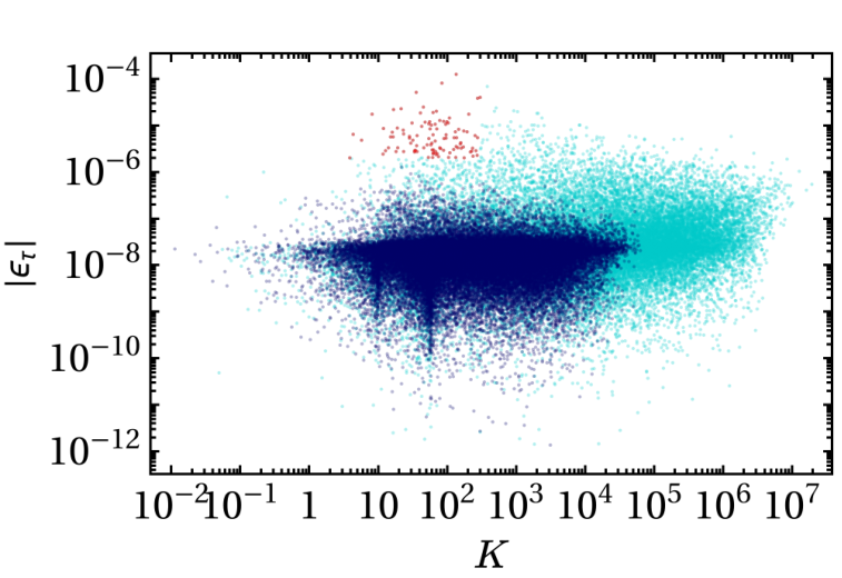
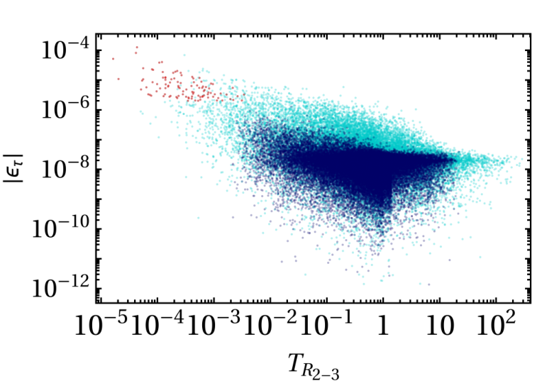
In an analogous manner, in the three-flavor regime analyzed in Sec. IV.2, a large breaking in the CP asymmetries of at least $|\delta\epsilon_{e}|\sim|\delta\epsilon|\sim 10^{-6}$ (cf. Figs. 2 and 3) in eq. (48) or for a small breaking in the flavor projectors, $(P_{\tau}-P_{\mu})/2\sim 0.1$, a CP asymmetry of at least $|\epsilon_{\tau}|\sim 10^{-5}$ was required. These contrast with the typical value of $|\epsilon_{\tau}|\sim 10^{-8}$ shown in the scatter plots of Fig. 6 that show the possible ranges for the $\mathsf{CP}^{\mu\tau}$ symmetric model. ⁵⁵ 5 We only show NO but IO is similar. The dark (light) blue points assume $|\xi_{i}|\leq 3$ ($|\xi_{i}|\leq 6$) for parameters $\xi_{i}$ that appears in the orthogonal matrix $R$ of the Casas-Ibarra parametrization; see explicit parametrization in Appendix D. The red points are a small subset of the light blue points with relatively large $|\epsilon_{\tau}|$ and moderate $K$, as can be seen in Fig. 6 (left). In contrast, Fig. 6 (right) shows $|\epsilon_{\tau}|$ against the ratio

$$T_{R_{2-3}}\equiv\frac{\sqrt{\sum_{i}(|R_{2i}|-|R_{3i}|)^{2}}}{\sqrt{\sum_{i}|R_{3i}|^{2}}}.$$

(57)

When this ratio is small, the second and third rows of $R$ are very similar in magnitude and this feature may be regarded as indication of fine-tuning or additional (approximate) symmetry. Also, when this ratio is small, the first row of $R$ is small in magnitude and this explains how the entries of $R$ may be large but $K$ is kept moderate . We can see that the red points are concentrated where the ratio is small which shows that fine-tuning is necessary to generate large $\epsilon_{\tau}$ but not too large $K$. We can then conclude that some fine-tuning (or additional symmetry) is required to achieve successful leptogenesis with small $\mathsf{CP}^{\mu\tau}$ breaking.

We can compare the tuning quantified in eq. (57) with other measures. Considering the type I seesaw formula in the basis $\nu_{L}\nu_{L}$,

$$M_{\nu}=-m_{D}^{\mbox{\scriptsize$\mathsf{T}$}}\hat{M}_{R}^{-1}m_{D}\,,$$

(58)

where $m_{D}=v\lambda$ and $\hat{M}_{R}$ is the right-handed neutrino mass matrix which is real, positive and diagonal. The seesaw naturally explains the light neutrino mass of order 0.1 eV for $\lambda\sim 1$ if $\hat{M}_{R}\sim 10^{14}\,\mathrm{GeV}$. Lighter right-handed neutrinos would require smaller $\lambda$ unless some cancellation kersten.smirnov between $m_{D}$ and $\hat{M}_{R}^{-1}$ takes place in the seesaw formula in eq. (58). The degree of cancellation can be roughly quantified by

$$T_{SS}\equiv\frac{v^{2}\|\lambda\|^{2}\lVert\hat{M}_{R}^{-1}\rVert}{\|M_{\nu}\|}\,,$$

(59)

where the double bars denote the matrix norm

$$\|A\|\equiv\sqrt{\operatorname{tr}[AA^{\dagger}]}=\sqrt{\sum_{ij}|A_{ij}|^{2}}\,.$$

(60)

The larger the measure of eq. (59) the larger the degree of cancellation. A similar measure is given by some norm of the matrix $R$ in the Casas-Ibarra parametrization aristizabal.

We will also see that to get large $|\epsilon_{\tau}|$, it is essential that we also consider the one-loop contribution to the neutrino mass matrix coming from Higgs and $Z$ in the loop:

$$M_{\nu}^{1{-}l}=m_{D}^{\mbox{\scriptsize$\mathsf{T}$}}\hat{M}_{R}^{-1}C_{\rm eff}(\hat{M}_{R})m_{D}\,,$$

(61)

where $C_{\rm eff}(\hat{M}_{R})$ is a function on the diagonal entries for which Mnu:1-loop

$$C_{\rm eff}(M)=\frac{M^{2}}{32\pi^{2}v^{2}}\left(\frac{\ln(M^{2}/m_{H}^{2})}{M^{2}/m_{H}^{2}-1}+3\frac{\ln(M^{2}/m_{Z}^{2})}{M^{2}/m_{Z}^{2}-1}\right)\,;$$

(62)

$m_{H}$ and $m_{Z}$ are the masses of the Higgs and the $Z$. The total neutrino mass matrix is then modified to

$$M_{\nu}=M_{\nu}^{\rm tree}+M_{\nu}^{1-l}\,.$$

(63)

Keeping $\hat{M}_{\nu}$ as the physical neutrino masses, one can include the one-loop contribution in the Casas-Ibarra parametrization by modifying the Yukawa coupling $\lambda$ to an effective $\lambda^{\rm eff}$ casas-ibarra:1-loop. See Appendix D for the expression. To quantify the relative contribution from the one-loop contribution, we further use  pascoli.turner

$$T_{loop}\equiv\frac{\sum_{i}\operatorname{SVD}(M_{\nu}^{1-l})_{i}}{\sum_{i}\operatorname{SVD}(M_{\nu})_{i}}\,,$$

(64)

where SVD denotes the singular values of the matrix. The larger this measure, the larger is the one-loop contribution, and if it is much larger than unity, it means that the tree and one-loop contributions are large but they largely cancel each other in (63).

References

- (1) M. Fukugita and T. Yanagida, Phys. Lett. B 174, 45 (1986).
- (2) S. Davidson and A. Ibarra, Phys. Lett. B 535, 25 (2002) [arXiv:hep-ph/0202239].
- (3) W. Buchmuller, P. Di Bari and M. Plumacher, Annals Phys. 315, 305 (2005) [arXiv:hep-ph/0401240].
- (4) E. Nardi, Y. Nir, E. Roulet and J. Racker, JHEP 0601, 164 (2006) [arXiv:hep-ph/0601084].
- (5) A. Abada, S. Davidson, F. X. Josse-Michaux, M. Losada and A. Riotto, JCAP 0604, 004 (2006) [arXiv:hep-ph/0601083].
- (6) A. Abada, S. Davidson, A. Ibarra, F.-X. Josse-Michaux, M. Losada and A. Riotto, JHEP 0609, 010 (2006) [arXiv:hep-ph/0605281].
- (7) B. Garbrecht, F. Glowna and P. Schwaller, Nucl. Phys. B 877, 1 (2013) [arXiv:1303.5498 [hep-ph]].
- (8) B. Garbrecht and P. Schwaller, JCAP 1410, 012 (2014) [arXiv:1404.2915 [hep-ph]].
- (9) A. Pilaftsis, Phys. Rev. D 56 (1997), 5431-5451 [arXiv:hep-ph/9707235 [hep-ph]].
- (10) A. Pilaftsis and T. E. Underwood, Nucl. Phys. B 692 (2004), 303-345 [arXiv:hep-ph/0309342 [hep-ph]].
- (11) K. Moffat, S. Pascoli, S. T. Petcov, H. Schulz and J. Turner, Phys. Rev. D 98 (2018) no.1, 015036 [arXiv:1804.05066 [hep-ph]].
- (12)
Special Issue on
“Neutrino Oscillations: Celebrating the Nobel Prize in Physics 2015”
Edited by Tommy Ohlsson,
Nucl. Phys. B 908 (2016) Pages 1-466 (July 2016),
http://www.sciencedirect.com/science/journal/05503213/908/supp/C. - (13) See for example, G. Altarelli and F. Feruglio, Rev. Mod. Phys. 82, 2701 (2010) [arXiv:1002.0211]; S. F. King and C. Luhn, Rept. Prog. Phys. 76, 056201 (2013) [arXiv:1301.1340]; H. Ishimori, T. Kobayashi, H. Ohki, Y. Shimizu, H. Okada and M. Tanimoto, Prog. Theor. Phys. Suppl. 183 (2010) 1 [arXiv:1003.3552 [hep-th]].
- (14) R. M. Fonseca and W. Grimus, JHEP 1409 (2014) 033 [arXiv:1405.3678 [hep-ph]].
- (15) F. Capozzi, E. Lisi, A. Marrone and A. Palazzo, “Current unknowns in the three neutrino framework,” arXiv:1804.09678 [hep-ph]; I. Esteban, M. C. Gonzalez-Garcia, M. Maltoni, I. Martinez-Soler and T. Schwetz, JHEP 1701 (2017) 087 [arXiv:1611.01514 [hep-ph]]; P. F. de Salas, D. V. Forero, C. A. Ternes, M. Tortola and J. W. F. Valle, arXiv:1708.01186 [hep-ph].
- (16) K. Abe et al. [T2K Collaboration], Nature 580 (2020) no.7803, 339 [arXiv:1910.03887 [hep-ex]].
- (17) P. F. Harrison and W. G. Scott, Phys. Lett. B 547, 219 (2002) [arXiv:hep-ph/0210197].
- (18) W. Grimus and L. Lavoura, Phys. Lett. B 579, 113 (2004) [arXiv:hep-ph/0305309].
- (19) R. N. Mohapatra and C. C. Nishi, JHEP 1508 (2015) 092 [arXiv:1506.06788 [hep-ph]].
- (20) Z. z. Xing and Z. h. Zhao, Rept. Prog. Phys. 79 (2016) no.7, 076201 [arXiv:1512.04207 [hep-ph]].
- (21) C. C. Nishi, B. L. Sánchez-Vega and G. Souza Silva, JHEP 1809 (2018) 042 [arXiv:1806.07412 [hep-ph]].
- (22) S. F. King and C. C. Nishi, Phys. Lett. B 785 (2018) 391 [arXiv:1807.00023 [hep-ph]].
- (23) H. J. He, W. Rodejohann and X. J. Xu, Phys. Lett. B 751 (2015) 586 [arXiv:1507.03541 [hep-ph]]; A. S. Joshipura and K. M. Patel, Phys. Lett. B 749 (2015) 159 [arXiv:1507.01235 [hep-ph]].
- (24) S. F. King and Y. L. Zhou, JHEP 1905 (2019) 217 [arXiv:1901.06877 [hep-ph]].
- (25) S. F. King, JHEP 1307 (2013) 137 [arXiv:1304.6264]; S. F. King, JHEP 1602, 085 (2016) [arXiv:1512.07531].
- (26) L. Covi, E. Roulet and F. Vissani, Phys. Lett. B 384, 169 (1996) [arXiv:hep-ph/9605319].
- (27) M. D’Onofrio, K. Rummukainen and A. Tranberg, Phys. Rev. Lett. 113, no. 14, 141602 (2014) [arXiv:1404.3565 [hep-ph]].
- (28) J. A. Harvey and M. S. Turner, Phys. Rev. D 42, 3344 (1990).
- (29) T. Inui, T. Ichihara, Y. Mimura and N. Sakai, Phys. Lett. B 325, 392 (1994) [arXiv:hep-ph/9310268].
- (30) N. Aghanim et al. [Planck Collaboration], “Planck 2018 results. VI. Cosmological parameters,” arXiv:1807.06209 [astro-ph.CO].
- (31) R. Samanta, R. Sinha and A. Ghosal, JHEP 1910 (2019) 057 [arXiv:1805.10031 [hep-ph]].
- (32) D. Aristizabal Sierra, L. A. Munoz and E. Nardi, Phys. Rev. D 80, 016007 (2009) [arXiv:0904.3043 [hep-ph]].
- (33) S. Antusch, P. Di Bari, D. A. Jones and S. F. King, Nucl. Phys. B 856 (2012) 180 [arXiv:1003.5132 [hep-ph]].
- (34) G. y. Huang and N. Nath, arXiv:2004.12391 [hep-ph].
- (35) R. Samanta and M. Sen, JHEP 01 (2020), 193 [arXiv:1908.08126 [hep-ph]].
- (36) G. D. Moore, Phys. Rev. D 62, 085011 (2000) [arXiv:hep-ph/0001216].
- (37) L. Bento, JCAP 0311, 002 (2003) [arXiv:hep-ph/0304263].
- (38) J. Casas and A. Ibarra, Nucl. Phys. B 618 (2001), 171-204 [arXiv:hep-ph/0103065 [hep-ph]].
- (39) I. Esteban, M. C. Gonzalez-Garcia, M. Maltoni, I. Martinez-Soler and T. Schwetz [NuFIT collaboration], 2018 results, http://www.nu-fit.org/?q=node/166.
- (40) J. Kersten and A. Y. Smirnov, Phys. Rev. D 76 (2007), 073005 [arXiv:0705.3221 [hep-ph]].
- (41) D. Aristizabal Sierra and C. E. Yaguna, JHEP 08 (2011), 013 [arXiv:1106.3587 [hep-ph]].
- (42) J. Lopez-Pavon, S. Pascoli and C. f. Wong, Phys. Rev. D 87 (2013) no.9, 093007 [arXiv:1209.5342 [hep-ph]].
- (43) J. Lopez-Pavon, E. Molinaro and S. T. Petcov, JHEP 1511 (2015) 030 [arXiv:1506.05296 [hep-ph]].
- (44) S. F. King and C. Luhn, Rept. Prog. Phys. 76 (2013) 056201 [arXiv:1301.1340 [hep-ph]].
- (45) S. Antusch, S. F. King and M. Spinrath, Phys. Rev. D 87 (2013) no.9, 096018 [arXiv:1301.6764 [hep-ph]]; S. F. King, JHEP 1307 (2013) 137 [arXiv:1304.6264 [hep-ph]]; Phys. Lett. B 724 (2013) 92 [arXiv:1305.4846 [hep-ph]].
- (46) F. Björkeroth and S. F. King, J. Phys. G 42, no. 12, 125002 (2015) [arXiv:1412.6996].
- (47) C. H. Albright, A. Dueck and W. Rodejohann, Eur. Phys. J. C 70 (2010), 1099-1110 [arXiv:1004.2798 [hep-ph]].
- (48) S. Choubey, S. F. King and M. Mitra, Phys. Rev. D 82 (2010) 033002 [arXiv:1004.3756 [hep-ph]].
- (49) C. S. Fong, Phys. Lett. B 752 (2016), 247-251 [arXiv:1508.03648 [hep-ph]].
- (50) K. Agashe, P. Du, M. Ekhterachian, C. S. Fong, S. Hong and L. Vecchi, JHEP 1904, 029 (2019) [arXiv:1812.08204 [hep-ph]].