On the connection problem for the second Painlevé equation with large initial data

The Painlevé equations are, in general, irreducible in the sense that their solutions cannot be expressed in terms of elementary functions or classical special functions. Therefore, the study on the asymptotic behavior of the Painlevé functions and their connection problem is a difficult topic in Painlevé theory. In this paper, we focus on the connection problem of the homogenous second Painlevé (PII) equation, i.e. the following equation:

$$\frac{d^{2}q}{dt^{2}}=2q^{3}+tq,$$

(1.1)

whose solutions are well studied. Although the “classic connection problem” for PII concerning solutions of (1.1) satisfying the boundary condition $q(t)\to 0$ as $t\to+\infty$ was given by Hastings and McLeod forty years ago [12], the PII equation (1.1) remains a research topic of great current interest due to its extensive applications in mathematics and mathematical physics. Recall that every Painlevé transcendent admits a Riemann-Hilbert characterization through the Stokes multipliers. In the case of the homogenous PII equation, the Stokes multipliers are subject to the constraints

$$s_{k+3}=-s_{k},~k\in\mathbb{Z},~{\rm and}~s_{1}-s_{2}+s_{3}+s_{1}s_{2}s_{3}=0,s_{1}=\overline{s_{3}},s_{2}=\overline{s_{2}}.$$

(1.2)

By collecting the results in the literature [4, 10, 12, 21], we know that, when $t\to-\infty$, the asymptotic behavior of the real-valued solutions of (1.1) are divided into three types according to the Stokes multiplier $s_{1}$:

1. (N1)

   If $|s_{1}|<1$, the solutions are oscillatory on the negative real axis, and satisfying

   $$q(t)=d(-t)^{-\frac{1}{4}}\cos\left(\frac{2}{3}(-t)^{\frac{3}{2}}-\frac{3d^{2}}{4}\ln(-t)+\phi\right)+\mathcal{O}\left((-t)^{-\frac{7}{10}}\right)\quad$$

   (1.3)

   as $t\to-\infty$, where

   $$d^{2}=-\frac{1}{\pi}\ln(1-s_{1}s_{3})\quad\text{and}\quad\phi=-\frac{3}{2}d^{2}\ln{2}+\arg\Gamma\left(\frac{1}{2}id^{2}\right)-\arg{s_{1}};$$

   (1.4)

2. (N2)

   If $|s_{1}|=1$, the solutions behave like

   $$q(t)=-\epsilon\sqrt{-\frac{t}{2}}+h(-t)^{-\frac{1}{4}}e^{-\frac{2\sqrt{2}}{3}(-t)^{3/2}}\left(1+\mathcal{O}\left((-t)^{-\frac{3}{2}}\right)\right)$$

   (1.5)

   as $t\to-\infty$, where

   $$h=-\frac{s_{2}}{2^{7/4}\sqrt{\pi}},\quad s_{1}=i\epsilon;$$

   (1.6)

3. (N3)

   If $|s_{1}|>1$, the solutions have an infinite number of poles on the negative real axis and

   $$q(t)=\frac{\sqrt{-t}}{\sin\left(\frac{2}{3}(-t)^{3/2}+\frac{3}{2}\beta\ln(-t)+\varphi\right)+\mathcal{O}\left((-t)^{-1/5}\right)}$$

   (1.7)

   as $t\to-\infty$, where

   $$\beta=\frac{1}{2\pi}\ln(s_{1}s_{3}-1)-1,\quad\varphi=3\beta\ln{2}-\arg\Gamma\left(\frac{1}{2}+i\beta\right)-\arg{s_{1}}.$$

   (1.8)

When $t\to+\infty$, the asymptotic behavior of the real-valued solutions of PII equation can be separated into two types according to the Stokes multiplier $s_{2}$:

1. (P1)

   If $s_{2}\neq 0$, the solutions (a two-parameter family) satisfy

   $$q(t)=\sigma\sqrt{\frac{t}{2}}\cot\left(\frac{\sqrt{2}}{3}t^{3/2}+\frac{3\gamma}{4}\ln{t}+\chi\right)+\mathcal{O}(t^{-1})$$

   (1.9)

   as $t\to+\infty$ with $\sigma=\text{sgn}(s_{2})=\pm 1$ and

   $$\gamma=\frac{1}{\pi}\ln|s_{2}|,\quad\chi=\frac{7\gamma}{4}\ln{2}-\frac{1}{2}\arg\Gamma\left(\frac{1}{2}+i\gamma\right)-\frac{1}{2}\arg(1+s_{2}s_{3})+\frac{\pi}{2};$$

   (1.10)

2. (P2)

   If $s_{2}=0$, the solutions (a one-parameter family) behave like the Airy functions to leading order, i.e.

   $$q(t)=\kappa\Ai(t)(1+\mathcal{O}(t^{-3/2}))$$

   (1.11)

   as $t\to+\infty$, where

   $$\kappa=-\im s_{1}.$$

   (1.12)

According to (1.3)-(1.12), one can build the connection formulas between the parameters in the asymptotic behaviors as $t\to+\infty$ and the ones as $t\to-\infty$. These connection formulas are well studied through the isomonodromy method [13, 23], the Deift-Zhou nonlinear steepest descent method [4, 8] and the uniform asymptotics method [1]. See [10] for a detailed summary of the connection formulas of PII and their applications.

The initial value problem of the inhomogenous PII equation with $(q(0),q^{\prime}(0))=(0,0)$ was analyzed through the isomonodromy method in [16]. To the best of our knowledge, it is the only case that the large $t$ asymptotic behaviors are explicitly connected with the initial data. Even so, some heuristic numerical results of the PII equation should be noted. For instance, it can be seen from [11, Figure 5] that the real solutions of the PII equation have $n(n=1,2,\cdots)$ poles on the positive real axis when their initial data locate on certain curves marked $n^{+}$. This means that these solutions belong to type (P2). Similarly, there exists a sequence of regions marked $n^{-}$ such that the solutions, whose initial data lies in these regions, possess $n$ poles on the negative real axis. Then they are type (N1) solutions. Nevertheless, it is to be further investigated on how to theoretically describe these curves and regions on the $(q(0),q^{\prime}(0))$ plane.

Recently, the initial value problem of the homogenous PII equation with real initial data $(q(0),q^{\prime}(0))$ have been numerically and analytically investigated by Bender et al.[2, 3]. They conclude that, when $q(0)=0$, there exist initial slopes $q^{\prime}(0)=b_{n}$ that give rise to the solutions of type (N2), where

$$b_{n}\sim\left[\frac{3\sqrt{2\pi}\Gamma(\frac{3}{4})n}{\Gamma(\frac{1}{4})}\right]^{\frac{2}{3}}\quad\text{as}\quad n\rightarrow\infty.$$

(1.13)

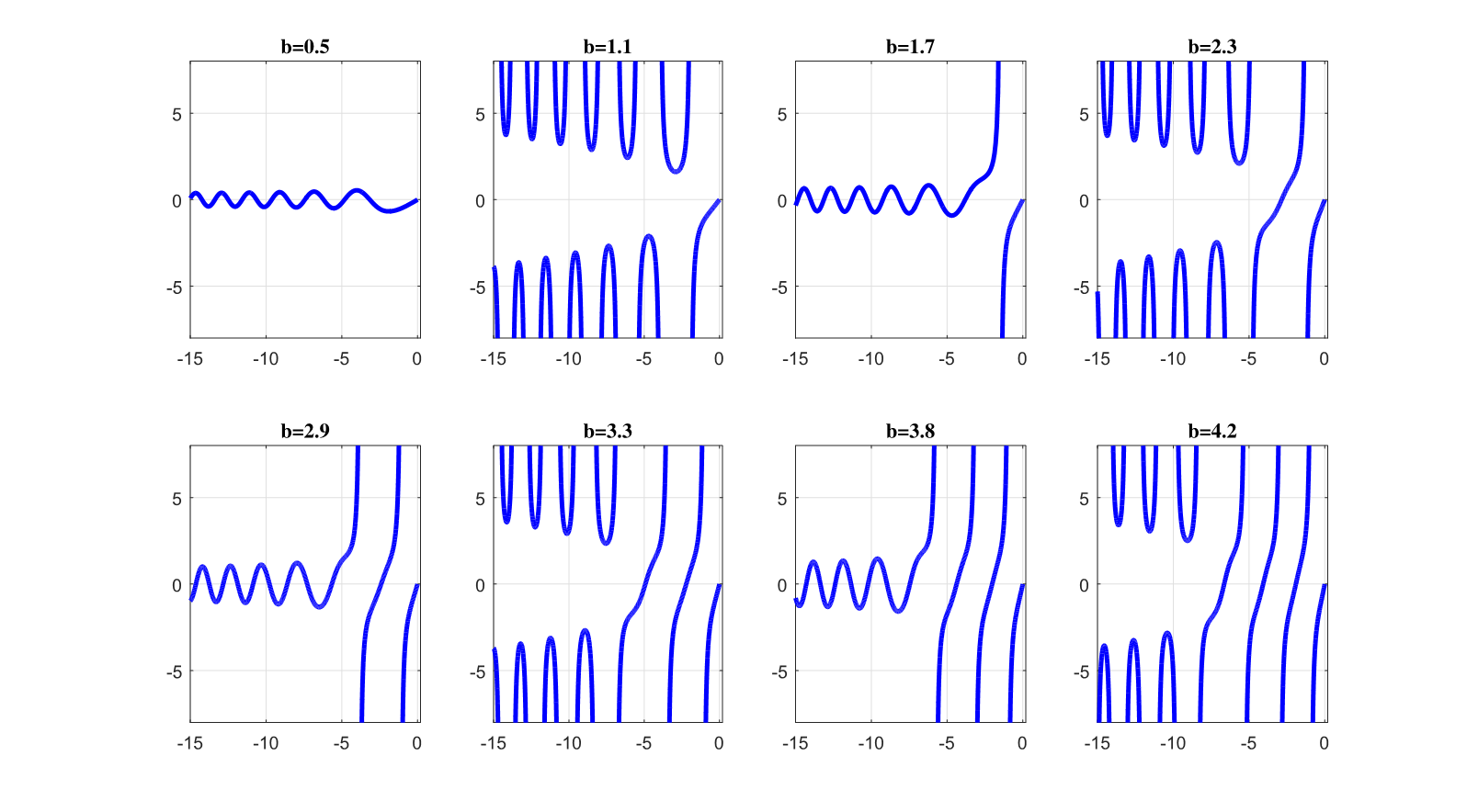
Moreover, a very interesting phenomenon appears as the initial slope varies. If $b_{2n}<q^{\prime}(0)<b_{2n+1}$, then the solution passes through $n$ simple poles and then oscillates stably on the negative real axis (type (N1) solutions), while for $b_{2n-1}<q^{\prime}(0)<b_{2n}$, the solution has infinite number of poles (type (N3) solutions); see Figure 1. It is similar when $q^{\prime}(0)=0$ and $q(0)$ varies; see [2, Figures 14 and 15]. We note that parts of the argument in [2, 3] are based on numerical simulations (see [2, p. 8]). In order to give a rigorous proof of their results and to build the connection formulas between the initial data and the large negative (positive) $t$ asymptotics, further analysis is needed.

Therefore, it is natural to consider the following initial value problem of PII

$$\begin{cases}\frac{d^{2}q}{dt^{2}}=2q^{3}+tq,\\ q(0)=a,~~q^{\prime}(0)=b,\end{cases}$$

(1.14)

where the initial data $a$ and $b$ are two real constants. The main task is to classify the PII solutions with respect to the initial data, or to build the connection formulas between the parameters involved in the asymptotic behaviors shown above in (1.3)–(1.12) and the initial data $a$ and $b$. Actually, as is well known, it is an open problem proposed by Clarkson on several occasions [5, 6, 7].

It seems difficult to completely solve Clarkson’s open problem for PII, nevertheless it is possible to give an asymptotic classification of PII solutions with respect to the initial data. Similar analysis for the first Painlevé equation (PI) has been investigated by Long et al. in [17]. By fixing the initial value $q(0)$, they have classified the real PI solutions asymptotically with respect to the initial slope $b$. The main idea is to compute the asymptotic behavior of the Stokes multipliers when $b$ is large. Similarly, when fix the initial slope $b$, the real PI solutions are classified asymptotically with respect to the initial value $a$.

The main objective of this paper is to give an asymptotic classification of the real-valued solutions of the homogenous PII equation (1.1) on the real axis with respect to the initial data. The key difference between the present paper and [2, 3, 17] is that we investigate how the asymptotic behaviors of the real-valued solutions of PII alternate when the initial data $a$ and $b$ are both varied. Note that $H(t)=\frac{1}{2}p^{2}(t)-\frac{1}{2}q^{4}(t)-\frac{1}{2}tq(t)^{2}$ is the Hamiltonian for the following Hamiltonian system of the PII equation

$$\left\{\begin{matrix}\frac{dq}{dt}&=\frac{\partial H}{\partial p},\\ \frac{dp}{dt}&=-\frac{\partial H}{\partial q},\end{matrix}\right.$$

(1.15)

where $p=\frac{dq}{dt}$; see [15, Table 4.2]. We regard $-2H(0)=a^{4}-b^{2}$ as a whole term and only assume that $a^{4}-b^{2}$ is large, instead of fixing $a$ or $b$. Set $a=\xi^{1/3}A(\xi)$ and $b=\xi^{\frac{2}{3}}B(\xi)$, where $\xi$ is a large positive real parameter and $A(\xi),B(\xi)$ are both real and bounded. Since $a^{4}-b^{2}$ can be large positive or large negative, we shall consider the initial value problem (1.14) in the following two cases:

	$\displaystyle({\text{i}})$	$\displaystyle A(\xi)^{4}-B(\xi)^{2}=1;$		(1.16)
	$\displaystyle({\text{ii}})$	$\displaystyle A(\xi)^{4}-B(\xi)^{2}=-1.$

In case (i), we obtain an asymptotic classification of the PII solutions on the positive real axis with respect to $a^{4}-b^{2}$, and in case (ii), we classify the PII solutions on the negative real axis similarly.

The main technique in this paper is based on the method of uniform asymptotics introduced by Bassom et al. [1], and further applied by [17, 18, 20, 24, 25, 26, 27]. To apply this method, we first briefly outline some important information of the monodromy theory of the PII equation. The reader is referred to [10, 14] for more details. One of the Lax pairs for (1.1) is the system of linear ordinary equations

$$\left\{\begin{array}[]{ll}\frac{\partial\Psi}{\partial\lambda}=\{-i(4\lambda^{2}+t+2q^{2})\sigma_{3}+4\lambda q\sigma_{1}-2q^{\prime}\sigma_{2}\}\Psi\\ \frac{\partial\Psi}{\partial t}=(-i\lambda\sigma_{3}+q\sigma_{1})\Psi.\end{array}\right.$$

(1.17)

Here and below the prime denotes the derivative with respect to $t$, and

$$\sigma_{1}=\left(\begin{array}[]{cc}0&1\\ 1&0\end{array}\right),~~\sigma_{2}=\left(\begin{array}[]{cc}0&-i\\ i&0\end{array}\right),~~\sigma_{3}=\left(\begin{array}[]{cc}1&0\\ 0&-1\end{array}\right)$$

are the standard Pauli spin matrices. A direct calculation shows that the compatibility condition $\Psi_{\lambda t}=\Psi_{t\lambda}$ implies (1.1). There exist canonical solutions $\Psi_{k}(\lambda,t)$, defined in a neighborhood of the irregular singular point $\lambda=\infty$, of the first equation of the Lax pair, with the following asymptotics behavior

$$\Psi_{k}(\lambda,t)=\left(I+O\left(\frac{1}{\lambda}\right)\right)\exp\left\{-\left(i\frac{4}{3}\lambda^{3}+it\lambda\right)\sigma_{3}\right\},~\lambda\rightarrow\infty,~\lambda\in\Omega_{k},$$

(1.18)

where the canonical sectors are

$$\Omega_{k}=\left\{\lambda\in\mathbb{C}\Big|\frac{(k-2)\pi}{3}<\arg\lambda<\frac{k\pi}{3}\right\},~k\in\mathbb{Z}.$$

(1.19)

These canonical solutions are related by

$$\Psi_{k+1}(\lambda,x)=\Psi_{k}(\lambda,x)S_{k},~\lambda\in\Omega_{k}\cap\Omega_{k+1},~k\in\mathbb{Z},$$

(1.20)

where $S_{k}$ are Stokes matrix defined by

$$S_{2j}=\left(\begin{array}[]{cc}1&s_{2j}\\ 0&1\\ \end{array}\right),\quad S_{2j-1}=\left(\begin{array}[]{cc}1&0\\ s_{2j-1}&1\\ \end{array}\right),\quad j\in\mathbb{Z}.$$

(1.21)

The Stokes multipliers $s_{k},k\in\mathbb{Z}$ are independent of $\lambda$ and $t$ according to the isomonodromy condition. As mentioned before, the Stokes multipliers are subject to the constraints (1.2).

The rest of this paper is arranged as follows. In Section 2, we state our main results in two theorems. In Section 3, the main theorems are proved with two lemmas to be shown later. In Section 4, we apply the method of uniform asymptotics to calculate the Stokes multipliers when $t=0$ and $\xi\to+\infty$ in the two cases in (1.16), and then prove the lemmas in Section 3. Some detailed calculations are left in the Appendixes.

When $A(\xi)^{4}-B(\xi)^{2}=1$ i.e. $a^{4}-b^{2}=\xi^{\frac{4}{3}}\to+\infty$, we have the following result.

Specially, in the case that the initial slope $y^{\prime}(0)=b$ is fixed, noting that $\xi$ is a large parameter and $A(\xi)^{4}-B(\xi)^{2}=1$, we find that $B(\xi)\to 0$ and $A(\xi)\to\pm 1$. Moreover, a simple calculation yields $\mathcal{F}(\xi)=\frac{\pi}{8}+o(1)$ when $B(\xi)\to 0$. Hence, the following corollary is a direct consequence of Theorem 1 and is consistent with the corresponding result mentioned in [3, p11].

When $A(\xi)^{4}-B(\xi)^{2}=-1$ i.e. $a^{4}-b^{2}=-\xi^{\frac{4}{3}}\to-\infty$, similar results are obtained.

The following corollary is a direct consequence of Theorem 2 and is consistent with the corresponding result mentioned in [3, p11].

According to the isomonodromy theory, a general idea to solve connection problems is to calculate the Stokes multipliers of a specific solution in the two specific situations to be connected. In the initial problem of PII, this means to calculate all $s_{k}$ when $t\rightarrow\pm\infty$ and $t=0$. When $t\rightarrow\pm\infty$, as stated above in (1.4), (1.6), (1.8), (1.10) and (1.12), the Stokes multipliers are well known. When $t=0$, it seems much more difficult to find the exact values of $s_{k}$. However, inspired by the ideas in Sibuya [22], we are able to obtain their asymptotic approximations in the special cases considered here, as a step forward. These approximations, together with (1.4), (1.6), (1.8), (1.10) and (1.12), suffice to prove our theorems.

When $s_{2}=0$, using the constraints of the Stokes multipliers in (1.2), we know that $s_{1}=\overline{s_{3}}$ and $s_{1}+s_{3}=0$ . Hence, we obtain $\im s_{1}=\mathbf{sgn}((-1)^{n+1}a)|s_{1}|$, which implies (2.1) immediately. When $s_{2}\neq 0$, it is readily seen from Lemma 1 that $\mathbf{sgn}(s_{2})=\mathbf{sgn}((-1)^{n+1}a)$ if $f_{n}(a,b)<a^{4}-b^{2}<f_{n+1}(a,b)$. Hence, substituting (3.1) into (1.10), we get (2.3). This finishes the proof of Theorem 1.

Similarly, according to the following lemma and corollary, one can easily get Theorem 2.

As an immediate consequence, we have the following corollary.

We leave the proofs of Lemmas 1 and 2 to the next section.

Let $\Psi_{k}=((\Phi_{k})_{1},(\Phi_{k})_{2})^{T},k\in\mathbb{Z}$ be independent solutions of (1.17), and set

$$\phi=\Big(4\lambda q-2iq^{\prime}\Big)^{-\frac{1}{2}}(\Phi_{k})_{2},$$

(4.1)

we get from (1.17) the second-order linear differential equation for $\phi(\lambda)$

	$\displaystyle\frac{d^{2}\phi}{d\lambda^{2}}$	$\displaystyle=\left\{-(4\lambda^{2}+t+2q^{2})^{2}+8i\lambda+(4\lambda q+2iq^{\prime})(4\lambda q-2iq^{\prime})\right.$
		$\displaystyle\left.\quad-\frac{4iq(4\lambda^{2}+t+2q^{2})}{4\lambda q-2iq^{\prime}}+\frac{3}{4}\frac{(4q)^{2}}{(4\lambda q-2iq^{\prime})^{2}}\right\}\phi.$		(4.2)

When $t=0$, equation (4) is simplified to

$\displaystyle\frac{d^{2}\phi}{d\lambda^{2}}$

$\displaystyle=\Big\{-\left(16\lambda^{4}+4a^{4}-4b^{2}\right)+4i\lambda+\frac{2b}{a}+\frac{i((b/a)^{2}-2a^{2})}{\lambda-\frac{ib}{2a}}+\frac{3}{4}\frac{1}{(\lambda-\frac{ib}{2a})^{2}}\Big\}\phi.$

(4.3)

Our task is to derive the uniform asymptotic approximation of the solutions of (4.3) as $\xi\rightarrow+\infty$. For convenience, we assume that $A(\xi)\cdot B(\xi)>0$, and the analysis is similar when $A(\xi)\cdot B(\xi)<0$ and only justified in a remark; (see Remark 4).

References

• [1] A. P. Bassom, P. A. Clarkson, C. K. Law and J. B. McLeod, Application of uniform asymptotics to the second Painlevé transcendent, Arch. Ration. Mech. Anal. 143 (1998), 241–271.
• [2] C. M. Bender and J. Komijani, Painlevé transcendents and PT-symmetric Hamiltonians, J. Phys. A, 48 (2015), 475202.
• [3] C. M. Bender, J. Komijani and Q. Wang, Nonlinear eigenvalue problems for generalized Painlevé equations. J. Phys. A, 52 (2019), 315202.
• [4] T. Bothner and A. Its, The nonlinear steepest descent approach to the singular asymptotics of the second Painlevé transcendent, Phys. D, 241 (2012), 2204-2225.
• [5] P. A. Clarkson, Painlevé equations-nonlinear special functions, J. Comput. Appl. Math., 153 (2003), 127–140.
• [6] P. A. Clarkson, Painlevé equations-nonlinear special functions, in Orthogonal Polynomials and Special Functions, Springer, Berlin and Heidelberg, (2006), 331–411.
• [7] P. A. Clarkson, Open Problems for Painlevé Equations, SIGMA, 15 (2019), 006, 20 pages.
• [8] P. A. Deift and X. Zhou, Asymptotics for the Painlevé II equation, Comm. Pure Appl. Math., 48 (1995), 277–337.
• [9] A. Eremenko, A. Gabrielov and B. Shapiro, High energy eigenfunctions of one-dimensional Schrödinger operators with polynomial potentials, Comput. Methods Funct. Theory, 8 (2008), 513–529.
• [10] A. S. Fokas, A. R. Its, A. A. Kapaev and V. Yu. Novokshenov, Painlevé Transcendents: The Riemann-Hilbert Approach, AMS Mathematical Surveys and Monographs, Vol. 128, Amer. Math. Society, Providence R.I., 2006.
• [11] B. Fornberg and J. A. C. Weideman, A computational exploration of the second Painlevé equation, Found. Comput. Math., 14 (2014), 985–1016.
• [12] S. P. Hastings and J. B. McLeod, A boundary value problem associated with the second Painlevé transcendent and the Korteweg-de Vries equation, Arch. Ration. Mech. Anal., 73 (1980), 31–51.
• [13] A. R. Its and A. A. Kapaev, The method of isomonodromy deformations and connection formulas for the second Painlevé transcendent, Math. USSR-Izv., 31 (1988), 193–207.
• [14] M. Jimbo, Monodromy problem and the boundary condition for some Painlevé equations, Publ. RIMS, Kyoto University 18 (1982) 1137–1161.
• [15] T. Kawai and Y. Takei, Algebraic Analysis of Singular Perturbation Theory, American Mathematical Soc., R.I., 2005.
• [16] A. V. Kitaev, Symmetric solutions for the first and second painlevé equations, J. Math. Sci. 73 (1995), no.4, 494–499.
• [17] W.-G. Long, Y.-T. Li, S.-Y. Liu and Y.-Q. Zhao, Real solutions of the first Painlevé equation with large initial data, Stud. Appl. Math., 139(2017), 505–532.
• [18] W.-G. Long, Z.-Y. Zeng, and J.-R. Zhou, A note on the connection problem of some special Painlevé V functions, Complex Var. Elliptic Eq. 62 (2017), 726–737.
• [19] F. W. J. Olver, D. W. Lozier, R. F. Boisvert and C. W. Clark (eds)., NIST Handbook of Mathematical Functions, Cambridge University Press, Cambridge, UK, 2010.
• [20] H.-M. Qin and Y.-M. Lu, Application of uniform asymptotics method to analyzing the asymptotic behaviour of the general fourth Painlevé transcendent, Int. J. Math. Math. Sci. 9 (2005), 1421–1434.
• [21] H. Segur and M. J. Ablowitz, Asymptotic solutions of nonlinear evolution equations and a Painlevé transcedent, Physica 3D, (1981), 165–184.
• [22] Y. Sibuya, Stokes multipliers of subdominant solutions of the differential equation y′′−(x3+λ)​y=0y^{\prime\prime}-(x^{3}+\lambda)y=0, Proc. Amer. Math. Soc. 18 (1967), 238–243.
• [23] B. I. Suleǐmanov, The connection of asymptotics on various infinities of solutions of the second Painlevé equation. Diff. Uravn., 23(1987), 834–842.
• [24] R. Wong and H. Y. Zhang, On the connection formulas of the third Painlevé transcendent, Discrete Contin. Dyn. Syst. 23 (2009), 541–560.
• [25] R. Wong and H. Y. Zhang, On the connection formulas of the fourth Painlevé transcendent, Anal. Appl. 7 (2009), 419–448.
• [26] Z.-Y. Zeng and Y.-Q. Zhao, Application of uniform asymptotics to the connection formulas of the fifth Painlevé equation, Appl. Anal. 95 (2016), 390–404.
• [27] Z.-Y. Zeng and L. Hu, On the connection problem for nonlinear differential equation, Bound. Value Probl. 2019(2019):73.