Hierarchical Predictive Coding Models in a Deep-Learning Framework
Abstract
Bayesian predictive coding is a putative neuromorphic method for acquiring higher-level neural representations to account for sensory input. Although originating in the neuroscience community, there are also efforts in the machine learning community to study these models. This paper reviews some of the more well known models. Our review analyzes module connectivity and patterns of information transfer, seeking to find general principles used across the models. We also survey some recent attempts to cast these models within a deep learning framework.
A defining feature of Bayesian predictive coding is that it uses top-down, reconstructive mechanisms to predict incoming sensory inputs or their lower-level representations. Discrepancies between the predicted and the actual inputs, known as prediction errors, then give rise to future learning that refines and improves the predictive accuracy of learned higher-level representations.
Predictive coding models intended to describe computations in the neocortex emerged prior to
the development of deep learning
and used a
communication structure between modules that we name the Rao-Ballard protocol.
This protocol was derived from a Bayesian generative model with some rather strong statistical
assumptions.
The RB protocol provides a rubric to assess the fidelity of deep learning models
that claim to implement predictive coding.
Here,
we consider the implementation of this protocol within convenient deep learning frameworks
that are robust to less restrictive statistical assumptions.
We employ deep learning examples to
demonstrate the feasibility and effectiveness of predictive learning.
Although neurally inspired in a historical sense, modern deep learning frameworks can be used at
an intermediate modeling level that is agnostic to specific claims about biologically based neural representations.
The intent is to make the classical models easier to study and more versatile and comprehensive while retaining
their core properties.
Keywords: Predictive coding, convolutional LSTMs, video frame prediction, generative models.
1 Introduction
Scientists have hypothesized that the brain, specifically the neocortex, acquires and updates internal representations by invoking learning mechanisms designed to predict incoming sensory input. These predictions are compared with actual sensory input to calculate discrepancies between input and predictions. These discrepancies, known as prediction errors, [37, 41, 16, 19] guide learning in the higher layers to reduce future prediction errors.
Although many forms of predictive coding have been proposed and found to exist in the brain [1], in regard to the neocortex, there are two main approaches toward building neural architectures for hierarchical predictive coding. The first, exemplified by the references cited above, uses a generative Bayesian approach, and is called Bayesian predictive coding [1]. In this approach, the higher layers learn to reconstruct the outputs of the immediately lower layers. Thus the higher layers, although represented more abstractly, contain the same information represented in the lower layers. The second approach, exemplified by the work of [34] and [2, 3], uses the higher layers to predict the prediction error in the immediately lower layer. This knowledge about the prediction error is used to modify the lower layer representation to reduce future prediction errors. The acquired representations are presumed to learn spatially and temporally immediate and distant causes or modulations of the input and this gives the representations their ability to predict future inputs.
Predictive coding models inspired by neocortex invariably use feedback from higher layers to lower layers. State-of-the-art deep learning models found in applied artificial intelligence rarely use feedback connections in their calculations. Both fully connected and convolutional deep networks are purely feedforward (what about semantic segmentation?). Recurrent networks, including gated recurrent networks, have lateral connections but not feedback connections [20] but not feedback connections across layers. The models in the deep learning literature which do have feedback connections are actually types of predictive coding models [34, 54, 23].
Feedback connections are ubiquitous in the neocortex. Virtually every feedforward connection from one cortical area to another is accompanied by a separate feedback connections linking those areas [14]. Both the feedforward connections and feedback connections consume significant brain volume and would not exist without an important functional reason. Predictive coding models, both Bayesian and non-Bayesian, offer attractive hypotheses for shedding light on the the computational purpose of feedback connections, as well as potentially offering significant improvements in deep learning performance.
As already mentioned, this type of learning has been called predictive coding, or more recently predictive processing [9, 27], and is usually described using a Bayesian generative model [31] where sensory input is combined with prior expectations, to make better future predictions. The term “predictive coding” predates Bayesian predictive coding. Non-Bayesian predictive coding has been used for other functions such as reducing information transmission requirements and cancelling the effects of self-generated actions [1].
Predictive coding can be usefully viewed as a type of representation learning [5]. The learning mechanisms to support Bayesian predictive coding should improve the quality of internal representations as a side effect of reducing future prediction errors. The predictive/reconstructive capacity ensures that the acquired representations can fully represent information contained in the input. Since learning is driven by prediction errors, the learning is unsupervised and simply requires a data stream of information to be predicted. [5] has noted that good representations are effective because they, in part, capture underlying “explanatory factors of variation behind the data”, and Bayesian predictive coding shares this goal.
In regard to applications, predictive coding networks can be used for learning overlapping image components [46], object classification [48, 54, 23], video prediction [34], video anomaly detection [56], modeling biased competition [45], response properties of primate visual cortex [41, 47], and EEG evoked brain responses [16] health concerns[57, 21]. It has also been proposed as a unified theory of neocortical function [18, 49, 27].
Its use in deep learning to build large models has so far been limited, with the models of [34], [54], and [23] being perhaps the only examples. Most predictive coding models have been implemented prior to the emergence of deep learning frameworks [41, 16, 46], so these classical models are small and do not use advanced modules for temporal processing, such as gated recurrent networks [22], now found in deep learning frameworks.
This survey explains some early predictive coding models and considers the question of enhancing them by using modern deep learning tools. We analyze the reasons for their effectiveness and offer proposals for future research. We also introduce a template for module connectivity which we call the Rao-Ballard protocol. We suggest that it can be used as a rubric to assess the fidelity of deep learning models that claim to implement predictive coding.
2 Hierarchical generative models and prediction error
2.1 Historical Motivation for Predictive Coding
An early motivation of predictive coding was to create models of the retina that had reduced information transfer requirements [49] because the optic nerve is a bottleneck in transferring visual information to the brain. Continuous visual input has high redundancy. If the cells on the retina calculated a moving average of the incoming light, both spatially and temporally, this would yield a prediction of the current input. By comparing the actual input with the prediction, the retina could send a prediction error to later processing areas, thereby reducing transmission bandwidth.
If the vertebrate retina created a representation of the current input image from scratch, the information transfer requirements would depend on the bandwidth needed to build a full representation of the current environment. However, the brain can generally make a very good prediction of the current state of the environment using its existing representations of the past environment along with constraints about how the environment tends to change. The prediction error might require much less bandwidth to represent than building a representation of the current envronmental state from scratch. If the brain already had a fairly accurate default prediction, then updating the default prediction with the prediction error could create an up-to-date representation with lower information transfer demands. Furthermore, it is plausible that prediction errors could provide good information to guide learning to improve the representation and reduce future prediction errors.
2.2 Bayesian Predictive Coding
A more recent attraction of predictive coding models is that they can be formulated in a generative [19] fashion, enabling them to predict sensory input. This is usually expressed as a hierarchy where a higher layer predicts the outputs of a lower layer (i.e., input to the higher layer) and any prediction errors provide information to guide learning in the higher layer. A hierarchical architecture involving feedforward and feedback connections is also consistent with the architecture of the primate neocortex [14]. In the context of perceptual inference and recognition, a trained generative model has the property that the learned representation can reconstruct the distribution of raw sensory inputs and estimate hidden causes in the input at different spatial and temporal scales. The reconstruction is possible because the learned representation(s) capture the causal factors that generated the input in the first place. It requires an inverse mapping from sensations to causes in order to construct the representation. This is challenging because computing the inverse mapping between sensations and causes in the physical world is an ill-posed problem, meaning that its solution is not unique. In a Bayesian approach, this can be addressed by using appropriate prior probabilities, which in some cases can be learned if given sufficient input. One way to do this is by learning to minimize prediction errors (i.e., predictive coding).
Early models of predictive coding were expressed as statistical models such as the hierarchical expectation maximization and variational free energy models used in [16]. Although these models presented an exact calculus for calculating predictions, the models presented challenges for further study because implementing the calculations was computationally intensive and the assumptions of the models were highly restrictive. In very recent work, the predictive coding idea has entered the realm of deep neural networks in the work of [8, 54], and [34]. This is significant because the large toolset that comes with deep learning frameworks can be employed in an off-the-shelf manner. Although such models sacrifice the exact Bayesian calculus, they can be specified as a deep neural network rather than an abstract statistical model. This allows the construction of more complex models. For example, the [34] model known as PredNet, links predictive error modules with convolutional LSTMs [42] and then uses a hierarchy of predictive error modules for next-frame video prediction. In PredNet, these components are all specified using the Keras deep learning framework with a few hundred lines of code.
Some ideas behind predictive coding resemble other types of deep learning models such as auto-encoders and deep belief networks. Auto-encoders are explicitly trained to learn representations that can reconstruct their input. Deep belief networks are built by stacking restricted Bolztmann machines (RBMs). RBMs in turn are trained to reconstruct their input. Comparison of these methods may uncover more universal principles but are beyond the scope of this survey.
3 Predictive coding to learn hierarchical context
Predictive coding models construct representation hierarchies by reducing prediction error across layers. There is more than one way to approach this depending on the nature of the representation that the higher layers are intended to construct. The first way is to construct increasingly abstract feature hierarchies, by using larger input context later in the hierarchy, similar to convolutional networks. The second way is to learn a hierarchy of higher-order errors as one would in a Taylor series expansion. Section 3.1 and 3.3 present examples of the first method. Section 4 presents an example of the second method.
3.1 The Rao/Ballard model
An early neural network demonstration of the context-based approach involves constructing a small feature hierarchy that models end-stopped neural receptive fields in primary visual cortex [41]. This is a landmark paper, is somewhat challenging to understand, and is the standard entry point to the literature on Bayesian predictive coding networks.
The network has three layers which is the minimum number of layers to exhibit acquired context effects. Each layer has two functionally distinct neural classes. These classes are internal representation neurons and prediction error neurons. Layer 2 error cells in the model simulate cells in primary visual cortex and capture context effects known to occur in some of these cells. Many response properties of some cells in primary visual cortex are determined by the structure of a feedforward input field, known as the classical receptive field, and these properties are not context sensitive. However, response properties of other cells can be affected by presenting stimuli that fall outside of the classical input region. These are called non-classical receptive field properties and are attributed to context effects assumed to come from either lateral or top-down feedback inputs which are outside the feedforward field. The phenomenon of end-stopping (i.e., orientation-tuned cell response decreases when spatial extent of stimulating input exceeds classical receptive field boundary; also known as “length suppression”) is one such effect. End-stopping is caused by surrounding context that is outside of the feedforward inputs to the the cell and cell firing rate, counter-intuitively, decreases when the size of a line or edge-shaped input grows larger than the width of the classical, feedforward receptive field. [41] show how this can be accounted for by predictive coding. The [41] model hypothesizes that this effect comes from feedback inputs originating in a layer that encompasses larger spatial context, and experimental evidence supports this [7].

[41] use a 3-level representation hierarchy where feedback from a higher layer conveys predictions of neural activity for the preceding layer. For instance, predicted activity in the lowest layer is compared with actual activity (raw sensory input). Prediction error is the output of a layer and is forwarded to the next higher layer. Within the hierarchy, there are two classes of neurons: internal representation neurons and prediction error neurons. Weight training is controlled by gradient descent on a cost function based on prediction error magnitude. End-stopping is modeled by letting the highest-level representation use adjacent spatial context when predicting the middle-level representation. The highest layer builds a representation for the larger spatial context.
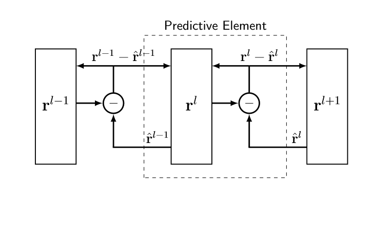
This model is built around the predictive element (PE). One can view the predictive element as a processing stage or cortical layer in the brain. In deep learning terminology, it consists of two neural layers performing complementary functions, and connected by both feedforward and feedback connections.
Predictive elements are stacked into a hierarchy (Fig. 1(a)). An element receives prediction errors (via forward connections) from the preceding layer in the hierarchy and sends predictions in the form of prior probabilities (via backward connections) to the preceding layer. In Fig. 1(a), we see the original view of the information flow. Layer learns a transformed representation of layer such that its prediction performance for layer ’s activity improves. The representation, , in a layer represents the hypothesized causes of the input, but at a higher level of description than the preceding layers. The different layers provide different representations of the same causes at increasingly higher description levels. The representation at each layer is manifested as a set of activation levels for the vector of neurons forming the layer.
Figure 1(b) refactors the drawing in part (a) to make the predictive error for a layer, , more explicit by using the symbol to represent prediction error and pairing it with a representation . This alternative view resembles that presented in [17] and [18]. The view in Fig. 1(b) shows that the interaction between adjacent layers obeys a constrained protocol which we will call the Rao-Ballard protocol because of its first implicit appearance in [41]. In our representation, there are four link types: prediction (P), prediction error (PE), lateral target (LT), and lateral target error (LTE). Layer output is the information provided by the PE link. The P and PE links are fully connected and the LT and LTE are point-to-point connections (see Fig. 2). Notice further that the representation modules only communicate with prediction-error modules and prediction-error modules only communicate with representation modules. Prediction error neurons never project downward in the hierarchy and internal representation neurons never project upward in the hierarchy. This view makes it easier to see the constraints imposed by the Rao-Ballard protocol. Fig. 1(b) poses an unanswered question: what kind of hierarchical representations are acquired in layers through and how do they compare with more traditional hierarchical representations obtained in deep learning models, such as convolutional networks?

Fig. 2 shows a network-level representation of a first-layer PE in [41]. For simplicity, the representation units in Layer 2, , are assumed to be linear. There are 256 inputs representing the input pixel intensities of a image patch but only 32 representation elements in the receiving layer, . The feedforward connections are in blue, , and the feedback connections, , are in red. The top-down prediction, denoted , is formed by calculating . The units calculate prediction error according to the formula . These ideas are related to the operation of the architecture and can be written
| (1a) | ||||
| (1b) | ||||
| (1c) | ||||
Eqn. 1a asserts several things. First, the input and the first layer representation are aliases. and both have dimensions (assuming a input image patch). The predicted input and the predicted representation are also aliases. The predicted input is given by , where has dimension and has dimension . Finally, under normal operating conditions, the input and the predicted input should be approximately equal.
Eqn. 1b simply defines the predictive error, , for Layer 1, as the elementwise difference between the actual and predicted input. Eqn. 1c is an equation for updating the internal representation in Layer 2 as a function of prediction error. We can derive Eqn. 1c as follows [40]. Start with a cost function, , on the sum-of-squared predictive error.
| (2) |
Since the equations are for a one-layer network, we leave out the layer superscripts for readability. This cost function does not take into account priors although the cost function reported in the original [41] model does incorporate priors. To prepare for gradient descent, we obtain the derivative of with respect to .
| (3a) | ||||
| (3b) | ||||
The intermediate step above uses the chain rule for vectors. For gradient descent, we travel in the opposite direction of the derivative at some rate, . This is shown below, were the update time steps, , are made explicit.
| (4) |
A more compact and convenient way of representing the above formula is shown in Eqn. 1c.
By taking the derivative of with respect to , an equation for learning in the network can be obtained is shown below.
| (5) |
Not shown in Figs. 1 and 2 is the option for higher layers to receive a wider range of inputs, either from adjacent areas of an input image, from complementary sensory modalities, or from a longer time scale. In these cases, the predictions sent back from the higher layer to the previous layer are influenced by broader context.
Given the module in Fig. 2, we want to see how the larger architecture looks and what happens when it is embedded within a context hierarchy, in our case, immediately adjacent spatial context. To achieve this, Fig. 3 extends Fig. 2 with two lateral PEs in the first layer (flanking the original patch module) and an added PE in the second layer. The input to Layer 2 consists of three overlapping image patches (patch overlap is 11 pixels, yielding a global input patch of ). Fig. 4 shows the overlapping image patches with a superimposed bar stimulus of two different sizes. The square with the solid outline shows the size of the receptive fields (RFs) representation units in Layer 1. The rectangle with the dashed outline shows the size of the receptive fields of the Layer 2 representation units.
The neurons – in Fig. 2 are the same neurons as those identified by – in Fig. 3. The newly added Layer 3 receives input from all PEs patches from Layer 1. Thus the receptive fields of representation units in Layer 3 are larger than those in Layer 2. In Fig. 3, the middle component of Layer 1 corresponds to the module in Fig. 2.


According to this model, endstopping phenomena occur in the prediction error neurons and reflects the reduced top-down prediction error associated with the longer line segment. Specifically, neurons – show reduced firing for the longer line on the right side of Fig. 4 because of the two lateral patch modules in the first layer. This is confirmed in the model by experiments which remove the feedback. This possible explanation of end-stopping was proposed in [37].
This paragraph out of place. The network was trained on several thousand natural image patches and the learning algorithm maximized the posterior probability of generating the input data. Thus, this is a generative model.
3.1.1 Problems with the Rao/Ballard model and future research
From a neuroscience viewpoint, the model has one problem.
- 1.
This problem concerns the information transfer requirements. It was stated earlier that a justification for predictive coding was the decreased bandwidth needed to send equivalent information. This is achieved in the feedforward direction. However, the full representation is sent in the feedback direction retaining the original bandwidth requirements. This may be an issue that all hierarchical predictive coding models must address.
One idea for future research is to directly measure the information transfer requirements (to address point 1) on a spiking version of this model. One could replace the continuous activation neurons with Poisson spiking neurons (or perhaps a more efficient spike coding scheme). By recording spiking events and measuring spike probabilities, we could directly measure the information transferred in model. We could compare the information transfer requirements for different coding schemes.
3.2 Predictive coding and divisive input modulation
Spratling [45, 46] used non-negative matrix factorization (NMF) to reformulate the [41] model of predictive coding to make it compatible with biased competition models of the brain. A related technique, known as divisive input modulation, offers promise of creating useful representations of subparts and is related to non-negative matrix factorization. [29] showed that NMF could create a useful object representation of, say faces, that consisted of local subparts resembling eyes, nose, and mouth.
More formally, consider a set of images represented as an matrix, named , whose entries are all non-negative values. The matrix contains images, . Each holds the set of non-negative pixel values for one image. The goal is to learn representations for the images by refactoring the matrix according to the constraint that all entries in the factors are non-negative. The refactoring takes the form below.
| (6) |
has dimension and has dimension . Think of as holding the feedback weights in a neural network and of as holding the transformed representation of each image within its columns. Its non-negativity constraints cause the matrix to be refactored into a parts-based representation. This is because the factorization only allows additive combinations [29]. Each column of is an internal representation of the corresponding image in Images. is the number of rows of and this determines the size of the representation. For instance, if using the example given in Fig. 2, would be 256 and would be 32.
[46] has shown that by changing the operators used in the predictive coding formulas, a method related to NMF known as divisive input modulation can be used which leads to some possible advantages over the [41] approach. Consider the revised predictive update equations shown below [48].
| (7a) | ||||
| (7b) | ||||
| (7c) | ||||
Eqn. 7a matches Eqn. 1a, except that it obeys the NMF constraint. Eqns. 7b and 7c match Eqns. 1b and 1c, except that they use different operators. Specifically, predictive error in Eqn. 7b is calculated using divisive input modulation, implemented by element-wise division (), instead of subtractive inhibition. For divisive input modulation, perfect reconstruction yields a value of one instead of zero. For Eqn. 7c, elementwise multiplication () is used instead of addition and this is an example of a multiplicative update rule [30]. Expressions of the form “” mean replace any values in that are smaller than with . For Eqn. 7b, this prevents division by zero and for Eqn. 7c this prevents any of the neurons from becoming permanently non-responsive. and are small positive numbers and example values to use in simulations can be found in [48].
The weight update rule uses multiplicative update and is shown below [46].
| (8) |
Recall that when there is no prediction error, is zero and the right side of the operator simplifies to one. is a rate parameter.
[30] provide batch-based algorithms for NMF, one of which minimizes the Kulback-Leibler (KL) divergence between the training and reconstructed images (). Whereas, the equations of Rao/Ballard are obtained by minimizing sum of squared error, the equations above minimize KL divergence.
[48] argues that his model has a number of advantages over the original [41] model. First, it can be implemented using only non-negative neural firing rates which makes it much easier to create bio-plausible implementations. Second, it is broadly compatible biased competition models [12] which also makes it easier to create bio-plausible implementations. Third, it has been argued that the proposed feedback connections of the Spratling model are more biologically plausible than those in the [41] model.
3.3 The Friston Free Energy Model
Following [41], [15, 16] developed a unified theory of sensory-based cortical function based on predictive coding which estimated the mean and variance of predicted states. This more general framework was based on the ideas of hierarchical expectation maximization (EM) and empirical Bayes (a method to estimate priors from data). This model is also biologically motivated along lines similar to [41], but is intended to address a broader range of empirical evidence [19]. The Friston model differs from [41], but still obtains the Rao-Ballard protocol. As the Friston papers are mathematicaly difficult, there is an authoritative tutorial of [6] that explains the Friston model and is essential reading to get started. Although Friston formulates this model using a statistical framework, our goal is to implement models of this type within deep learning frameworks that scale to larger problems and, in practice, require fewer statistical assumptions. We use the [6] variant of the Friston model.
As mentioned earlier, building representations which capture causes of sensory input, such as the shapes, reflective characteristics, arrangements and movements of objects, [48, p. 151] is a type of inversion process. In the real world, this calculation may be intractable or impossible (ill-posed) because the inverse is not unique. This can happen because of nonlinear interactions among the causes, for example visual occlusion [16, p. 816]. This problem can be handled by estimating what the prior distribution should look like. Why? See Rao/Ballard, 1997 [16] uses empirical Bayes to obtain these priors.
Let us calculate the most likely value of a continuous quantity, given sensory evidence. Following [6], we use a concrete perceptual inference problem, namely, inferring the amount of a food item in the environment from the intensity of its projection on the retina. The scalar variables and denote the pixel intensity and food amount, respectively. The problem is formulated probabilistically, as . This denotes the probability that the random variable (food quantity) has some value, given the pixel-intensity variable has some value. We wish to compute the most likely value of , given a specific value for the sensory input, , and the prior . This is known as an MAP estimate. Bayes’s rule,
| (9) |
lets us find the most likely value of , denoted , by maximizing the log of the numerator (also known as negative free energy11 1 [16, p. 821] observes that “minimizing the free energy is equivalent to minimizing a precision weighted sum of squared prediction error.”) on the right-hand side (RHS) of the equation below, that is
| (10) |
Let us assume that and are normally distributed, where . denotes the value of with the most likely prior probability and denotes the variance of the prior distribution. Similarly, we assume . Equation 10 can be expanded by substituting the formulas for these probability distributions.
Function predicts the raw sensory input (e.g., image pixel values) from the representation by using a causal observation model. This takes the form of a deteministic, usually nonlinear function of denoted and which may contain trainable parameters, .
| (11) |
is some representation of causes (e.g., amount of food), is some representation of the raw sensory input, and is a set of parameters (likely learnable) used to configure . To develop intuitions, one can think of as a deterministic causal process that takes the state of the environment and maps it to . An alternative interpretation is that is a function that the brain can learn to approximate and the input to is a representation, , which resides in the brain but models causal effects in the environment. The output, , of can then be viewed as a prediction of what the sensory input should look like. Although, in general is nonlinear, for this exposition we assume that is linear. For simplicity, we assume that .
Our next steps for developing the scalar version of the free energy model are the following.
- 1.
Develop equations to find the maximum of by performing gradient descent. Performing gradient descent on the resulting equations is called predictive activation update. In appropriate contexts in can be called inference (in contrast to learning).
- 2.
Represent the equations in Step 1 as a neural network such that the trainable parameters map to weights or synapses in the network and the other parameters of the network map to neuron like elements (nodes) that can have activation levels.
- 3.
Use to develop learning rules for the weights in the network.
One way to maximize is to perform gradient ascent on with respect to the estimated most likely value . The derivative of is
| (12) |
Next, refactor this formula by defining two types of prediction errors involving and .
| (13a) | ||||
| (13b) | ||||
With these prediction error definitions, Eqn 12 is rewritten as,
| (14) |
letting us express the problem of maximizing in terms of prediction error. For a given parameter set, gradient descent on Eqn. 14 can be used to search for an optimal value of .

Note that the neural model has been factored so that prediction errors are explicit nodes in the network as seen in Fig. 5. The derivatives needed for gradient descent to update the nodes in the network are given as follows.
| (15a) | ||||
| (15b) | ||||
| (15c) | ||||
Eqn. 15a says that update to the representation activations depends on the difference in prediction error for two consecutive layers. Eqns. 15b and 15c are obtained from 13a and 13b by moving to the RHS, setting the derivative on the LHS to zero, and then simplifying the RHS. After convergence of gradient descent, the network reaches a state which maximizes with respect to the current parameter values.
Fig. 5 shows a possible neural implementation of this model. The circled variables indicate continuous-valued, single neuron activations. The black lines ending with arrowheads and solid circles indictate excitatory and inhibitory neural connections, respectively. The red arrows point to synaptic contacts where learning occurs. The variables u, , , and are modeled as neural activations. The labeled connections between the neurons , , , and are the values of the weights at the synaptic contacts and can be trained. The trainable parameters have been made explicit by associating them with synaptic contacts.
The last step is to develop learning rules to train the network. Learning equations for the five synapses are given below. They are obtained by taking the derivative of with respect to the relevant synaptic parameter.
| (16a) | ||||
| (16b) | ||||
| (16c) | ||||
| (16d) | ||||
Notice that all of the resulting learning rules are in some way functions of predictive error. The prior probability, , is not changed unless there is predictive error related to prior (Eqn. 16a). For Eqns. 16a and 16d, there is no learning when the predictive error is zero and learning increases with higher predictive error. For Eqns. 16b and 16c, the variance decreases when the predictive error is zero.
Fig. 5 has two synapses with the same label, . Their separate weights are matched, in the sense that they each use the same learning rule, but not shared (they are different synapses). The model can be simulated by running all of the dynamic equations simultaneously.
Running the network, given an input stimulus to be processed, requires three steps as shown in the free energy algorithm below.
Performs network update (inference) and learning.
- 1.
Initialize the network with sensory input.
- 2.
Perform predictive activation update (inference) by gradient ascent using Equation Set 15 for some fixed number of integration steps (e.g., Forward-Euler), or until the node activations converge.
- 3.
Apply learning rules in Equation Set 16 to update the network weights.
The algorithms of [54] and [23], described in Section 5.1, show possible ways to do the above in a deep learning framework for convolutional networks.
This model can be generalized to multiple variables and multiple layers. The node dynamics and learning are governed by multidimensional versions of the rules already described. The generalized model uses multivariate instead of univariate Gaussian distributions. Also, the distinction between and is generalized to and , where and stand for consecutive layers. This is seen in Fig. 1 (b).
Predictive update dynamics are now specified using indexed equations across layers , namely, a pair of coupled equations for each level in the hierarchy conforming to Fig. 1(b). The symbols in [41] correspond approximately to the symbols in the equation below. By extracting the couplings, we recover the Rao-Ballard protocol (see Fig. 6).
| (17a) | ||||
| (17b) | ||||
Eqn. 17a calculates the representation component in Fig. 1(b) and Eqn. 17b calculates the predictive error for that layer. Eqn. 17a has two additive terms on its RHS. These approximately correspond to the information flowing on the incoming links to in Fig. 1(b). Because of the couplings, we see that receives input from both and . These correspond to the links LTE and PE in the Rao-Ballard protocol. Similarly, receives inputs from and in the protocol. These correspond to the links P and LT in the protocol. Fig. 6 helps visualize this information. Priors are represented on the P links.


Equation Set 17 is numerically simulated by updating each equation across all layers for each time step. For reasons discussed in Section 5.1, we call this a global update procedure. Besides the links used in the Rao-Ballard protocol, we should also note the recurrent connections. Eqn. 17a has a self reference in the second additive term on the RHS. Eqn. 17b also uses a recurrent connection in the third additive term on the RHS.
The next section considers the question of using these equations and the RB protocol as a guide to build a deep predictive coding network. In a deep learning framework, the protocol constraints can be realized by ensuring that the both the and modules are implemented as recurrent networks. Also, Equation Set 17 is intended to operate on feature vectors and a deep learning model will be applied to next-frame video prediction. Therefore, must adjust the model so that it operates on multi-channel images.
In the spirit of [41], [15, 16] formulates this setup hierarchically intending to capture different levels of representation that might occur in the brain. A given level provides priors to the immediately lower level to support Bayesian inferences. The model outline is shown below.
| (18a) | ||||
| (18b) | ||||
| (18c) | ||||
The higher-level representations, , predict the state of immediately lower-level representations, . at the lowest level denotes observed values at the sensory receptor. Each function is deterministic with its own parameter set . The ’s add noise to the predictions.
By adding assumptions about the noise sources being Gaussian with covariance , we can reformulate Eqns. 18 probabilistically. The equation below expresses the likelihood of given the state of .
| (19) |
and are now vectors of continuous variables and is sampled from a multi-variate Gaussian distribution with mean and variance . The representation at level provides priors for level providing top-down expectations to the lower layer.
Before proceeding, let us review EM in a nonhierarchical context. The EM learning algorithm is iterative with two steps in the iteration loop: the E-step and the M-step. The E-step uses the recognition equation below to assign probability values to the causes, , of a given input, , using the current parameter values, .
| (20) |
Using Bayes’s rule, this equation computes the probability of a cause given the current input and the current parameterization of the model, , which will be adjusted in the M-step. The rule inverts the generative formula , which predicts the input distribution. If the value of formula 20 can be computed tractably, the model is said to be invertible. Otherwise, it is noninvertible [11] and relates to the ill-posed nature of sensory input mentioned at the start of this section. In the context where the model is not invertible, we introduce an approximate recognition distribution written
| (21) |
which uses a new parameter set, , called recognition parameters.
We of course need a way to estimate this approximate distribution. Predictive coding is a form of EM that finesses the challenge of finding the parameters for complicated recognition densities. In a predictive coding framework, the parameters “are dynamically encoded by the activity of units in the brain” [15, p. 1339].
The M-step uses the results of the E-step to update the model parameters, and this is how learning occurs. In traditional EM, the specific update equations depend on the details of the particular causal model used. A common didactic example to illustrate EM is to use a Gaussian mixture model to generate data which is to be clustered. In this case, the parameter set consists of: 1) the mixture proportions; 2) the mean vectors of each distribution in the mixture; and, 3) the parameters for the variance of each mixture distribution. The specific details of such causal models can be arbitrarily complicated. Predictive coding is a version of EM that avoids the challenges of formulating and parameterizing specific causal models.
According to [16], EM is “a useful procedure for density estimation that has direct connections to statistical mechanics” [p. 820].
4 Predictive coding in a deep learning framework
[8] may have been the first to use the term “deep predictive coding networks.” However, the model of [34], named PredNet, may be the earliest predictive coding model implemented using a deep learning (DL) framework. Implementing a predictive coding model using a DL framework has a number of potential advantages over implementing the direct mathematical formulations described earlier. DL frameworks are very mature, versatile, and efficient. Consequently, they should make it easier to build and study predictive coding models, with the only complication being their ability to handle cross-layer feedback connections. Second, models using DL frameworks scale to very large architectures with over one hundred thousand parameters. This has not been achieved using traditional implementations of predictive coding. Third, deep learning architectures allow the use of large learning modules (such as LSTMs) that can cope with more relaxed statistical assumptions and, thereby, operate in more general situations. For instance, they allow us to drop strong assumptions such as Gaussian priors. Since PredNet is the first predictive coding model implemented using a DL framework, we shall discuss this model in detail.
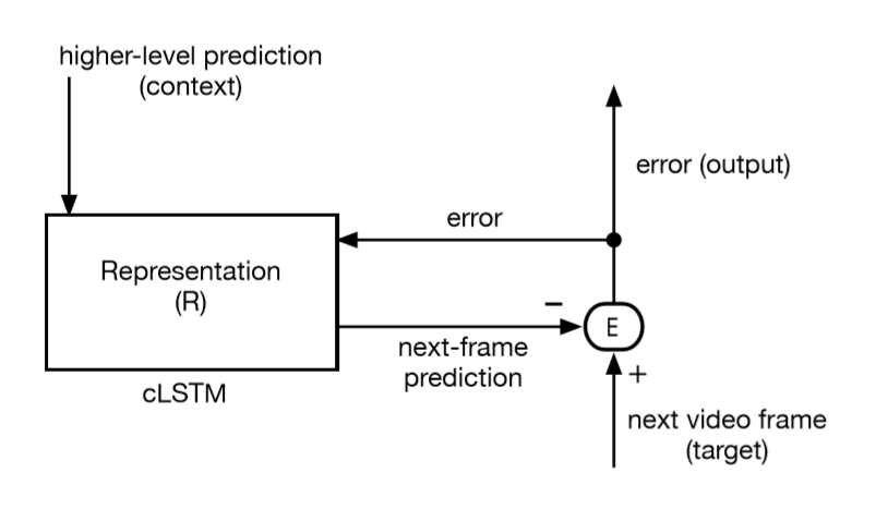
PredNet falls into the second category of models mentioned in the introduction. That is, it predicts prediction error. It is applied to the task of next-frame video prediction. Because PredNet manipulates video data, the representation modules in this model consist of convolutional LSTMs (cLSTMs) [42]22 2 A convolutional LSTM is an LSTM whose internal data structure is a multichannel image.. LSTMs are recurrent networks with trainable gating operations to help them remember or forget different types of relevant or irrelevant past information when performing sequence processing. The internal data structure that they manipulate is a feature vector and this is suitable for applications like natural language processing. cLSTMs are a modification of LSTMs that use multi-channel images as their internal data structure in place of feature vectors. Accordingly, cLSTMs replace gate operations based on affine weight multiplication (used in regular LSTMs) with convolutional gate operations that apply to multi-channel images. This allows them to develop useful representations of image sequences such as video.
Fig. 7 shows a PredNet predictive element for the lowest layer of the model where the representation module on the left is implemented as a cLSTM. By using the cLSTM, PredNet’s architecture generalizes predictive coding models to perform more complex tasks than, say, that of [41]. Note that the output of the representation module projects to the error calculation module, which sends its output back to the representation module. The model learns to predict the next frame in a video (target) by comparing its prediction with the target frame and using the prediction error as a cost function. Since Fig. 7 does not show how the feedforward and feedback connections link to the next higher layer, we cannot determine whether it is a model that predicts prediction error. At this point, it is generic as a predictive coding model.
Although, PredNet is inspired by predictive coding principles, its design diverges fundamentally from the models of [41], [16], and [46]. The most noticeable difference is that it uses cLSTMs to implement the representation modules instead of layers of neurons.
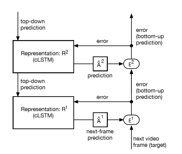
A more subtle and fundamental difference between PredNet and the earlier models is that the intermodule connectivity in PredNet diverges from the previous models we have examined. Specifically, PredNet does not use the RB protocol. This cannot be readily seen in Fig.7, but is more apparent in Fig. 8(a) which shows a two-layer version of the model. The module interconnectivity pattern differs from the RB protocol. For example, the second-layer representation projects to the first-layer representation, whereas, if using the RB protocol, it would project to the first-layer error. Similarly, if using the RB protocol, the first-layer should project to the second-layer representation. Instead it projects to the second-layer error.
Let us examine intuitively how PredNet works when a new video frame is given to the network. We start with the lowest layer. The representation layer () generates a prediction for the next video frame on the basis of the knowledge encoded in its weights. The prediction is sent to the error module () via the convolution module () which modifies the dimensions coming from so that it matches the error module. The error module also receives the target, which is the actual video frame that appears next in the sequence. The error module computes prediction errors by performing two subtractions. The prediction is subtracted from the target (e), and the prediction error is sent back to the representation, as well as to the next higher layer. Similar to the previous models [41, 6], the error module is subtractive.
Learning adjusts the weights for the convolutional filters as well as the weights for the internal gates within the cLSTM.
The error modules, , in the model are subtractive as in the previous models [41, 6]. When the representation and error modules are combined, they form a network layer as shown in Fig. 7. These layers can be stacked and a two-layer version of the model is shown in Fig. 8(a). In this figure, the inter-layer connectivity becomes apparent. The network weights are trained by backpropagation where the cost function is a weighted sum of the prediction errors generated by the modules for all of the layers. For the four-layer version of their network, they used two versions of a training loss function, and , which are based on how the are weighted.33 3 In the [34] model, these loss weightings are static throughout training, in the earlier models discussed they are dynamically weighted according to the calculated precision. For the loss, the four are weighted as . The loss uses which gives a small weighting to each of the higher layers. The model performed slightly better when the loss was used, which means that incorporating loss in the high-level modules, very surprisingly, reduced performance quality.
Once trained, their model predicts the next frame in a video sequence after seeing some number of previous frames in the sequence (e.g., 10). The model uses a hierarchy of predictive coding layers with bottom-up (feedforward) and top-down (feedback) connections. The feedforward connections convey prediction errors to the error module in the next higher layer and the feedback connections convey representation updates to the representation module in the previous layer (see Fig. 8(a)). The prediction at the lowest layer is intended to predict and match the next frame in the video sequence. Characteristic of deep learning, the model uses convolutional and recurrent (cLSTM) modules. As such, it is an important contribution that merges deep learning with predictive coding.
First, as seen in Figure 8a, the feedforward connections project to prediction error neurons instead of representation neurons. Second, the feedback connections project to representation neurons and not prediction error neurons. Both of these properties depart from the Rao-Ballard protocol used in the above mentioned models.
Specifically, the prediction error for a lower layer is sent directly to the error calculation for the next higher layer in contrast to the Rao-Ballard protocol where prediction error would be sent to the next higher representation layer. The representation for a higher layer is sent to the representation for the previous layer in contrast to the Rao-Ballard protocol where it would be sent to the error calculation for the previous layer. Thus, PredNet diverges from the earlier predictive coding models.
We now present the training cycle for the architecture. This can be compared with the Free Energy algorithm in Section 3.3.
Performs network activation update during training. Operates on one frame of input in a video stream. Model attempts to predict the next video frame and calculates prediction error. An activation update step is described below.
- 1.
Input current video frame.
- 2.
Perform top-down update sweep on the representations.
- 3.
Perform bottom-up update sweep on the predictive errors.
Weight update is controlled by backpropagation on the mean absolute error (MAE). MAE is calculated by summing the prediction errors across layers and the previous history ten steps into the past. Backpropagation is applied to reduce MAE.
The [41] model showed how larger spatial context from a higher layer can provide information to a lower layer to reduce prediction error. Although the [34] model provides higher-level feedback from a higher layer representation module to the previous layer representation module, the nature of the information provided is different. The representation module in the second layer of the Lotter model (see Fig. 8(a)) appears to be trained (more explanation shortly) to predict the prediction error generated by the first layer. That is, it is not being trained to predict the input to the lower layer, as was the case for previous models. This means that the nature of the higher-level information provided is different. It provides information to predict the prediction error and it is not obvious how this is useful in actually reducing prediction error. There is a missing link in the theory. Heuristically, it seems counter intuitive and [34] do not provide a rationale for making this choice. Although there is evidence that the model gives good performance, there is not a well articulated theory of why this model functions.
Let us analyze Fig. 8a to try to develop a theory of how the model functions. We focus on how the two-layer model should be better than the one-layer model. When using the training loss, the error value is not part of the training loss function, so learning in the representation at Layer 2 only reduces the loss . The hedge “appears to be trained” used in the previous paragraph relates to this. The network architecture suggests that level-two representation is reducing higher-order error, but the loss function contradicts this. Since is not influencing the training, The information for the backpropagated weight updates, originating with , flows in the opposite direction that the arrows point.
Hypothesis: If we cut the link labeled “1”, it should have a negligible effect on performance. If this hypothesis turns out to be true, then the higher-level predictive error calculations perform no significant function. This would mean that the Lotter model is not really a predictive coding network, and that its principle of function is similar to that of a traditional deep network. Specifically, it is a hierarchical cLSTM network that uses sum-of-squared error loss at the lowest layer.
Although not explicitly shown in the figures, pooling is used on the upward links and upsampling is used on the downward links between consecutive layers. This implements some form of hierarchical spatial context but, as mentioned above, it is difficult to heuristically interpret by virtue of it treating prediction error as the higher-level representation.
The unit activations in the model do not have obvious probabilistic interpretations but the model does appear to be generative in the way that it creates its next frame predictions.

4.1 Modifying the Lotter Model to use the Rao-Ballard Protocol
Because of the novelty of the [34] model’s design, it is useful to compare the original [34] model with a version that obeys the more established Rao-Ballard protocol. This comparison has not yet been performed. Thus, we propose a novel revision to [34] so that its module connectivity conforms to the Rao-Ballard protocol which can be used as a baseline to evaluate the original model. Our revised deep-learning-based architecture, which is heuristically similar to the [41] or [16] design, is shown in Fig. 9. It should be compared with Fig. 8(b). The original [34] model uses top-down feedback to directly update the next lower representation. The version that incorporates the Rao-Ballard protocol uses the top-down information as a prediction that enables prediction error to be computed. The loss function used for training should be .
Fig. 9 depicts a novel model not yet studied. It differs form the original [34] model in two ways. First, vertical links between the representation components and between the error components are dropped. Thus, there are no direct feedback connections between representations in consecutive layers. Direct feedforward connections between error modules in consecutive layers is also dropped. Second, horizontal links between the representation and error components are added. So, the representation in a given layer receives input from the error module in the current layer and also from the error module in the previous layer. This figure should also be compared with Fig. 1(b). This model matches the original heuristic intentions of the Rao-Ballard protocol although we do not supply a formal probabilistic interpretation.

4.2 Potential for bioplausibility
Recent simulation experiments have been conducted in an effort to support the biological plausibility of the model [35, 53].
The Lotter et al. model predicts several neuroscience phenomena [35, 53] including the time-course of neural firing rates after stimulus onset, end-stopping and other phenomena related to non-classical receptive fields, and a number optical illusions. Regarding firing rates, neurons exhibit an on/off temporal dynamics in regard to presenting and removing visual inputs in some parts of the visual cortex (area V2). This applies to stimuli to which the neuron is tuned. Such neurons have a low baseline firing rate before stimulus presentation. After stimulus onset, the neuron’s firing rate transiently increases and then returns to baseline. After returning to baseline, the same neuron’s firing rate will transiently increase when that same stimulus is turned off. This naturally fits a predictive coding interpretation where the neuron becomes active in response to prediction failures (It predicts constancy in the stimulus). [35] have shown that artificial neurons within prednet can exhibit this behavior at a population level (but not at an individual neuron level). They presented PredNet with static inputs of a range of naturalistic objects at time-step zero. Then they removed the stimulus at time-step six. When averaged over the stimuli and units for a given layer, the population response matched the response dynamics of primate V2 neurons. This is consistent with the interpretation that the population dynamics of PredNet were operating within a predictive coding regime. It also suggests analogies between the function of PredNet and the visual cortex.
[35] and [53] have shown that PredNet can account for some visual illusions. These include illusory contours, the flash-lag illusion, and illusory motion in static images. [53] showed that PredNet can predict illusory motion. This phenomenon arises when motion is perceived in static images. For examples, see Akiyoshi’s illusion pages http:www.ritsumei.ac.jp/~akitaoka/index-e.html. These experiments were conducted because previous papers suggested that predictive coding offered an explanation of motion illusions [38, 39, 43]. One important aspect of this study is the methods they introduced to analyze effects of the predictive coding mechanism within the network. Their most impressive analysis was an optical flow analysis used to guide image [36] registration for predicted images as a means measure the predicted motion in consecutive image frames.
4.3 Additional potential for bioplausibility
As stated earlier, other representations can be used in place of the convolutional LSTM. The convolutional LSTM can be replaced by a reduced-gate network which, under some circumstances, gives comparable performance with fewer parameters [13]. It can also be replaced by an Inception-based LSTM [26].
More biologically plausible alternatives are possible. [10] developed an LSTM that uses subtractive gating (because subtractive inhibition exists in the brain, Fig. 5), instead of multiplicative gating. If this subtractive LSTM were extended to be convolutional, then it would be a candidate to be used in the [34] model to increase its bioplausibility. Possible research idea. In another vein, [47] and Section 3.2 explored using divisive inhibition (versus subtractive inhibition) as a more bioplausible means of implementing predictive coding. This could be incorporated in [34].
4.4 Significance of the Lotter model
The [34] model may be the first predictive coding model implemented within a deep learning framework. This model is much larger and more comprehensive than using a formally specified statistical model (e.g., [16]). It moves in the nonparametric direction, dropping specific statistical assumptions like Gaussian priors. The free-energy principle is as compatible with deep learning models as it is with formally specified statistical models. [41] used a neural network implementation but because they did not have access to a deep learning development environment, they were limited in the size, complexity, and variety of the models they could study.
4.5 Revising the Lotter Model
[34] used an architecture which forwarded prediction errors as a prediction for the next level in the hierarchy. The [41] model did this also. They differ in where the representation information for a given layer is sent. For [41], the representation information is used to compute prediction error for Layer , whereas [34] uses that information to compute the prediction error for Layer .
The [34] representation acquired in Layer is trained to reduce only prediction errors from the previous layer. It seems that the [34] model is trained to acquire a hierarchy of high-order errors.44 4 A loose analogy to the Taylor series might provide intuition here. Think of the higher layers as corresponding to the higher-order derivatives of the Taylor expansion. It is not clear that these higher order derivatives would be useful in a representational context. The [41] design seems better suited to acquire a representation hierarchy.
Open questions and possible further experiments:
- 1.
Does the Lotter model give state-of-the-art video prediction performance? There do not appear to be comparisons with other approaches.
- 2.
Quantifying the effect of the number of layers. The [34] model was applied to two data sets using five (face rotations data set) and four layers (KITTI traffic data set), respectively. However, their short paper did not quantify the effect of adding more layers. Experiments should be done to confirm that adding more than one layer does indeed improve performance and the potential improvement should be quantified. Without these experiments, we do not know for a fact that the larger spatial context of higher layers improves performance on these data sets. If this is not confirmed, the predictive coding theory associated with the model is meaningless.
- 3.
Experiments with moving MNIST [50], as well as our own experiments with the Lotter model, show that it is easier to predict the movement of the digits than it is to predict their shape (even though digit shape is fixed). One could say that the digit shapes are low-pass filtered but this is not very informative. It only says there is information loss in the system. Why is it so hard for this version of the architecture to acquire knowledge of digit shape? What needs to be added? Maybe position information is less memory intensive and that some form of auto-encoder functionality should be added to encode shape.
- 4.
Analysis of prediction accuracy. It was pointed out earlier that the [34] model lacks a clear theory of why the model functions. We must understand what predictive information is learned in the representation module. In regard to movement (but not shape), measuring optical flow (using the CV2 library) between the representations of consecutive images may help. Our own experiments lack this analysis. Four types of comparisons would help.
- (a)
An optical flow comparison between predicted and target images. This would give detailed information about the mismatch between the predicted and target images and could serve as a cost function that is more informative than the SSE cost function.
- (b)
An optical flow comparison between the previous and current target. This would give ground truth information about how the image changes.
- (c)
Comparison between the previous target and current prediction. Combining this with information from item b, gives information about how the predictions go wrong.
- (d)
Visualizations of within-channel optical flow in the representation module could reveal quantitative information about the properties of the internal representations. Is optical flow the same for all channels?
- (a)
- 5.
Increasing bio-plausibility. Many papers offer hypotheses [4, 43] citations about how predictive coding can be implemented in minicolumns. We should compare these with PredNet and similar models. If we built a subtractive convLSTM, would that work in the Lotter model? Which is more compatible with the minicolumn hypothesis: the original Lotter model, or the model modified to use the Rao-Ballard protocol?
- 6.
Improving Prednet by using trainable upsampling. The top-down feedback in the Prednet implementation uses the Keras UpSampling2D API. This just resizes the image. Performance may be improved by instead using the Conv2DTranspose API which has trainable weights. This allows search to find the best upsampling to reduce the cost. This increases the parameter budget and may require more training data to prevent overfitting.
5 Predictive update can improve classification
Except for [48], the previously discussed models have not been used for classification. Predictive update (inference) is the second step in Free-Energy Algorithm . A pair of studies has shown that predictive update can improve the performance, of convolutional feature hierarchies [54, 23], including better state-of-the-art classification accuracy, faster convergence time, and the need for fewer layers.
When using a feedforward hierarchy of feature representations, the presumption is that the representation in each layer within the hierarchy should use different features.55 5 With some exceptions such as ResNet layers which are bypassed because of skip connections. Consider two consecutive layers, and , which are fully and bidirectionally connected, have the same number of units, and also have identical linear activations, that is, the representations are identical. If the feedback connections from to implement the identity transform, then layer can perfectly reconstruct the representation in . In this case, there is no prediction error to trigger learning, and the higher-layer representation is stable [55]66 6 There are empirical results [23] described later in this section that the representation converges under predictive update. when identical to the lower-layer representation. When identical, there is no need to have both layers in the hierarchy. Additional constraint must be added to the system, most likely at layer , to make the representations in consecutive layers different, so that deep learning is useful. That is, some constraint must be imposed on layer so that, while it uses layer to create a representation, it is forced to create a different (higher-level) representation.
To set up a baseline predictive coding model within a deep learning framework for classification, consider a feedforward convolutional architecture with layers. Now extend the standard feedforward convolutional architecture to include predictive coding by adding feedback connections to each layer. The feedback connections originating in layer use the representation in layer to reconstruct and predict the representation in layer . Prediction errors are communicated forward from layer to layer and these errors guide learning (minimize reconstruction errors by gradient descent on error) of the feedforward and feedback weights to reduce future reconstruction errors. We will call this the basic PredCode architecture.
5.1 The Purdue group and predictive activation update
A pair of studies [54, 23] from Purdue introduced the above basic PredCode architecture. They added predictive activation update, similar to that described in Section 3.3, into deep convolutional architectures. They compare identical deep learning architectures with and without predictive activation update so that the effects can be assessed. It was found that predictive activation update yields faster learning convergence and better classification accuracy as compared to the plain deep-learning versions of these networks when tested on data sets like CIFAR, MNIST, and SVHN, regardless of whether the predictive activation update is global or local. Their results also show that predictive activation reduces the need for extremely deep feature hierarchies. These predictive coding networks were less than ten layers deep. The improved prediction accuracy remained even when the number of parameters between the plain and PCN versions were held constant.
5.1.1 Adding predictive update to a baseline convNet
The first study mentioned above, [54], used a global version of predictive update. This method propagates the updates throughout the hierarchy for each update cycle. They studied visual classification problems on the data sets mentioned above and started with a baseline VGG-like CNN classification architecture [44] that was upgraded to use global average pooling [33]. This was called the plain CNN. The enhanced network was called predictive coding net (PCN). PCN was directly compared to the plain CNN and achieved the improved results described at the beginning of Section 5.1.
To add predictive update functionality to the plain CNN, [54] introduced recurrent processing for each pair of consecutive layers of the network like that suggested in Section 5 to build the basic predictive coding architecture. They derived their equations for a fully connected network although their actual implementation used a convolutional network. Working within the framework of a fully connected network with linear layers, they started with the equations below to compute prediction error:
| (22a) | ||||
| (22b) | ||||
The above equations are consistent with the [41] Eqns. 1a and 1b, except that they are formulated to apply in a hierarchical context. denotes the feedback weight matrix originating in layer and projecting to layer . Unlike Eqn. 1a, it is not required that be equal to . is the prediction error for layer , where is the feedback prediction from layer . By examining the communication within and between layers and , we see that it uses part of the Rao-Ballard protocol, namely, the P and LT links (Fig. 1). Later, we will see that it also uses the P link as seen in Fig. 10. However, it does not use the LTE link. When comparing with Equation Set 1, we see that the update equation has not yet been specified.
To obtain the recurrent update equations, we take the derivative of the loss with respect to the representation activations for a particular layer, , to set up gradient descent. Following Eqn. 2, the loss for layer is given as:
| (23) |
The derivative of the loss with respect to changes in the activation level of representation neurons in layer is given below. The process for predictive activation will cycle between feedforward and feedback updates. Eqn. 24a will be used to derive feedforward updates and follows the derivation in Equation Set 3. Eqn. 24b will be used to derive feedback updates.
| (24a) | ||||
| (24b) | ||||
The derivatives above give us a means to perform the predictive activation update step (Step 2) in Free-Energy Algorithm . They are used in the gradient-descent-based feedforward and feedback update equations given below where we have substituted the derivatives and simplified.
| (25a) | ||||
| (25b) | ||||
Eqn. 25a is used for the feedforward update and it matches Eqn. 4 and uses the same rate parameter . Eqn. 25b is used for the feedback update in the recurrent cycle and does not have an equivalent in the [41] model.
These equations can also be compared with the free-energy model in Section 3.3. They have a similar purpose to those in Eqn. 17a and serve as an example of implementing a free-energy-like network within a convolutional deep learning framework. Updating this recurrent set of equations corresponds to implementing the equivalent of Step 2 of Free-Energy Algorithm . In contrast to the free-energy model, the loss function is different and does not formally incorporate priors. This latter point seems to be the most important difference from the free-energy model. The PCN model generates predictions from the next higher layer to the preceding layer. This is intuitive and natural, but these predictions come from a convolutional network which does not formally incorporate prior probabilities. Although the model minimizes prediction errors, the prediction errors do not appear to be based on prior probabilities.
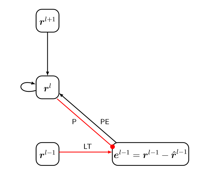
The data flow diagram in Fig. 10 shows the information flow for the predictive update step for layer in the [54] model. The shown connectivity is based on Equations Sets 22 and 25. When compared with Figs. 1(b) and 6(b), we see that it does not use the Rao-Ballard protocol. Specifically, its use of top-down information is different and this indicates that it treats prior information differently.
5.1.2 The global prediction error learning algorithm
We now describe how the above equations are incorporated into the predictive update cycle. The steps below present the PCN algorithm for one batch of training. Learning occurs only in Step 3 and this step uses a standard, backpropagation based algorithm. The similarities of this PCN algorithm to the Free-Energy Algorithm in Section 3.3 are fairly clear. Also, this algorithm is similar to the [34] algorithm with the exception that is constrained to be one.
[Global Version] Operates on one input batch, , of a convolutional network.
- 1.
Perform feedforward convolutional sweep on .
- 2.
Do recurrent activation updates, both feedforward and feedback, over all layers for () timesteps. The intention is to use updates to converge the network activations to a minimum prediction error. An expanded description is given below.
- 3.
Update all weights, including feedback weights, according to cross-entropy classification loss.
Informally, the feedforward sweep in Step 1 initializes the activations for the entire network. The predictive update in Step 2 refines these activation levels. The feedforward weights are shared between Steps 1 and 2. The feedback weights are only used in Step 2. Updates in Step 2 are determined by gradient descent on the predictive error. Following these two steps, Step 3 occurs where all weights (feedforward and feedback) are trained by gradient descent on the cross-entropy classification loss. Since the recurrent network is unrolled, the weight updates affect both the feedfoward and ultimately the recurrent weights. Note that the classification error (cross entropy), and not prediction error, controlls the weight updates. On the subsequent batch, the new feedforward sweep initializes the activations to improved values as a result of the training on the previous cycle.
Steps 1 and 3, without Step 2 (or ), in PCN Algorithm 5.1.2 above is a plain feedforward algorithm with gradient-based learning on a convolution network for one input batch. The novelty of global PCN lies in Step 2 where the recurrent updates take place. To see why the above is a global algorithm, we examine the details of the recurrent updates in Step 2. The algorithm below expands Step 2 and is performed for iterations where is a small integer-valued hyperparameter.
Expansion of Step 2 in PCN Alg 1: Performs predictive activation update for one time step.
- 1.
- 2.
This is considered global update because each loop in Steps 1 and 2 traverse all of the layers in the network and can propagate the effects of any layer to an arbitrary number of layers forward or backward.
To summarize, the top-down component (Step 1) computes predictions for each layer (except the top layer) and then updates the activations of those layers to take into account the predictions. Since the predictions for layer will ultimately depend on the updated activations for Layer via Layers , , …, this is a global algorithm. Updates for a higher layer can in principle influence updates for a lower layer a long distance below. A similar long-distance effect can occur in the activation updates from the bottom-up sweep. For these reasons, the authors describe the predictive update algorithm as global.
5.1.3 Local prediction error model
[23] replaced the global predictive update scheme described above with a local scheme that prevented predictive update effects from propagating to earlier layers in the network. The modified network’s classification performance did not suffer from this restriction, suggesting that the original long-distance, top down information flow had a negligible effect on the original performance. There are some caveats in drawing this conclusion, however, because other aspects of the architecture were changed from the global model. The original VGG-like architecture was replaced with a ResNet-like architecture having skip connections. The ResNet architecture may have compensated for removing the global aspect of the predictive update. Also, this local architecture used batch normalization, which is known to improve performance, whereas global average pooling was used in the previous architecture.
The local model’s design has much in common with the global model. The architecture is a feedforward convolutional network extended with recurrency and it uses the same predictive update equations (Equation Set 25). As in the global model, the recurrent steps are unfolded in time to transform the network into a feedforward achitecture. The full feedforward sweep can be broken down as: 1) the classic feedforward sweep and 2) the unrolled recurrent sweep (which becomes feedforward). The predictive activation equations are the same as in the global model, namely Equation Set 25.
Training the local model
To see how the local model differs from the global model, we examine the network activation and training algorithm more closely. A bottom-up sweep performs the recurrent updates between the lowest pair of consecutive layers for times steps, and then repeats the process for the next higher layer. Unlike PCN Algorithm 5.1.2, there is no top-down sweep. The algorithm is shown below. Weight-update learning occurs in Step 2.
[Local Version] Operates on one input batch, , of a convolutional network.
- 1.
Perform bottom-up forward sweep. For each layer and starting with Layer up to layer do:
- (a)
Layer relu(conv2D(batchNormalize layer ))
- (b)
Do recurrent activation updates for time steps on Layers and to compute the converged activations of Layer .
- (c)
Add a skip connection from Layer to via a bypass convolution.
- (a)
- 2.
Update all weights according to cross-entropy classification loss.
The bottom-up sweep constrains the effect of the predictive activation updates to affect activations only at a higher layer (and not lower layers). The details of the recurrent updates in Step 1b are given below.
Expansion of Step 1b in PCN Alg 2: Performs predictive activation update for one local recurrent time step on Layers and .
- 1.
Apply Conv2DTranspose to Layer to generate prediction for Layer . Denote it by .
- 2.
Compute prediction error for Layer by subtracting from the activations, . Denote the prediction error by .
- 3.
Add to the activations in Layer .
In the above, the conv2D in Step 3 uses the same weights as Step 1(a) of the overview. There is a difference because in Step 1(a) the input is the activations of Layer and the input for Step 3 is the prediction error. That is, the same weights are used for two different purposes.
5.2 Summary of predictive update with convolutional networks
The previous section reviewed two papers, known as PCN models, that introduced predictive update into deep convolutional architectures. The predictive update served to fine tune the network activations to reduce prediction error after the initial feedfoward sweep. Gradient descent on the classification loss (cross entropy) was used to adjust the weights after the fine tuning. For the model that used global predictive update, PCN Algorithm 5.1.2, the steps in the algorithm are quite similar to those in Free-Energy Algorithm . Both algorithms perform predictive update in Step 2 and weight training in Step 3.
In the PCN models, predictive update seems to prevent information loss from the representations in the lower layers to the higher layers. By improving the ability of the higher layer to predict the representation activations in the lower layer, the updated representation in the higher layer improves information preservation of the information contained in the lower layer. In a plain convolutional network without predictive activation, the only factor influencing weight update is the cross-entropy loss function designed to maximize classification accuracy. This goal of learning only what is needed for the immediate classification event could filter information deemed irrelevant to the classification task, yet may be still relevant to longer term learning.
Delete?
A deep network using shared weights across layers can be viewed as a shallow recurrent network [32].
How many training cycles did it take to converge?
For the local version, 300 epochs with batch size of 128, and initial learning rate of .
Compare the trained feedfoward weights between the normal and enhanced architectures. The bypass connection in [23] adds the representation in layer to that of layer .
Mutual information. Measure the mutual information between adjacent layers before and after predictive update. This is a way to test whether predictive update reduces information loss.
6 Design for revised Lotter et al. model using RB protocol
This appendix specifies more details of the RBP-PredNet model and initial experiments comparing it to the original PredNet [34]. Although our RBP model uses the same modules as the original PredNet, their communication is reconfigured to match the RB protocol. Fig. 11 shows design details for a 3-layer version of our model. In addition to the module input connectivity, the figure shows the number of input and output channels for each module. This provides enough information to calculate the parameter count as seen in Table 1.
All trainable parameters are in the , , and modules. All three module types perform multi-channel, 2D convolutional operations. The and modules use one operation, whereas the module, because it is a convolutional LSTM, uses four sets of identical operations. If the number of output channels is , then multi-channel convolutions are required to calculate this output, and this is the size of the convolution set. The convolutional LSTM has three gate operations and one input update operation, each of which calculates one multi-channel convolution set.77 7 Recurrent and nonrecurrent inputs are stacked, and this contributes to the number of input channels. These sets are identical, except for the weight values in their kernels. The number of input channels, denoted , to an module is the sum of the feedforward, lateral, and feedback inputs. All convolutional operations use square filters with kernel size on one dimension denoted by . Taking these factors into account, the formula below gives the parameter count for a set of multi-channel convolutions, henceforth called a convolution set.
| (26) |
Above, the number of weights for a multi-channel, convolutional filter is given in parentheses. Each filter has one bias. For each output channel, one multi-channel convolution is needed. Table 1 illustrates the calculation for the Fig. 11 model and reveals that the model has 65,799 trainable weights.

We will compare the Fig. 11 RBP model with a 3-layer version of the original Lotter et al. design that is shown in Fig. 12. Both variants use the same eleven modules. Both models are constrained to use the same output channels in the modules. However, to make the modules fit together, this entails that the input channel counts for the modules are different, as well as the channel counts for the and modules, and the and modules bridging them. Since the input channel counts are different, the Fig. 12 model has 103,020 parameters (cf., Table 2), instead of 65,799.
The arrows connecting the modules in both figures show direction of information flow. Numeric labels on the arrows show channel counts for that path. The number of output channels in the modules for each model are matched. However, the output channel count in the modules is less for the RBP model. The image dimensions for the three layers also match. There are more parameters in the Lotter et al. model than in the RBP model. This is because the number of parameters is primarily controlled by the number of input channels to the modules.
In both models, the module has three channels because of the RGB image encoding. The output channels for the modules separately encode positive prediction error and negative prediction error, so the number of output channels is twice the number of input channels.
| Parameter Count for RBP Model | ||||||
| # of conv | filter | input chans | output chans | Calculation | parameter | |
| Module | sets | () | () | count | ||
| 1 | 3 | 3 | 84 | |||
| 4 | 15 | 3 | 1,632 | |||
| 1 | 3 | 3 | 84 | |||
| 1 | 12 | 3 | 327 | |||
| 4 | 42 | 12 | 18,192 | |||
| 1 | 12 | 12 | 1,308 | |||
| 1 | 24 | 12 | 2,604 | |||
| 4 | 48 | 24 | 41,568 | |||
| Total parameters: | 65,799 | |||||


| Parameter Count for Lotter et al. PredNet Model | ||||||
| # of conv | filter | input chans | output chans | Calculation | parameter | |
| Module | sets | () | () | count | ||
| 1 | 3 | 3 | 84 | |||
| 4 | 21 | 3 | 2,280 | |||
| 1 | 6 | 12 | 660 | |||
| 1 | 12 | 12 | 1,308 | |||
| 4 | 60 | 12 | 25,968 | |||
| 1 | 24 | 24 | 5,208 | |||
| 1 | 24 | 24 | 5,208 | |||
| 4 | 72 | 24 | 62,304 | |||
| Total parameters: | 103,020 | |||||
Method. All models were trained for twenty epochs, using the Adam optimizer, on the preprocessed KITTI traffic data set used in [34]. This data set was preprocessed by [34] to obtain three-channel color images of size pixels. Successful prediction on this dataset requires the model to detect and track several moving and nonmoving objects in a video frame.
Three architectures were tested. The first was the RBP architecture where the modules were built from convolutional LSTMs. The second was the RBP architecture where the modules were built from convolutional GRUs. The third was tested using the original [34] architecture. Two sets of loss function weights were used, namely, and .
Several architectures were tested as specified in Table 3.
The first experiment used the loss function weights with values . The second experiment used loss function weights with values . Two experiments were performed. We also studied a GRU based version of the RBP model. This replaced the LSTMs in the modules with GRUs.
For all experiments, three performance measures were recorded: mean absolute error (MAE), mean squared error (MSE), and structural similarity index (SSIM). All measures were calculated on a baseline control condition [34] for comparison with the neural network performance measures. The baseline used the current video frame as the prediction for the next frame.
| Model Parameters as a Function of ID | |||||
|---|---|---|---|---|---|
| Model ID | R type | stack_sizes | R_stack_sizes | Loss weights | Params |
| Pred1 | LSTM | [3, 12, 24] | [3, 12, 24] | [.5, .4, .2] | 103,020 |
| Pred2 | LSTM | [3, 12, 24] | [3, 12, 24] | [1.0, 0, 0] | 103,020 |
| RB1 | LSTM | [3, 3, 12] | [3, 12, 24] | [.5, .4, .2] | 65,799 |
| RB2 | LSTM | [3, 3, 12] | [3, 12, 24] | [1.0, 0, 0] | 65,799 |
| RB3 | LSTM | [3, 12, 24] | [10, 16, 30] | [1.0, 0, 0] | 162,641 |
| RB3_gru | GRU | [3, 12, 24] | [10, 16, 30] | [.5, .4, .2] | 125,523 |
| RB4_gru | GRU | [3, 12, 24] | [10, 16, 30] | [1.0, 0, 0] | 125,523 |
| RB5 | LSTM | [3, 3 , 12] | [ 3, 12, 24] | [.33, .33, .33] | 65,799 |
| RB6 | LSTM | [3, 3] | [ 3, 12] | [1.0, 0] | 9,951 |
| RB7 | LSTM | [3, 3] | [ 3, 12] | [.5, .5] | 9,951 |
| Model | Model | MAE | MAE | MAE | MSE | SSIM |
|---|---|---|---|---|---|---|
| Type | ID | train | valid | predict | predict | predict |
| Baseline | .0757 | .0212 | .6750 | |||
| Lotter | Pred1 | .0187 | .0243 | .0694 | .0162 | .7138 |
| RBP | RB1 | .0191 | .0245 | .0704 | .0163 | .7116 |
| RBP_gru | RB3_gru | .0195 | .0245 | .0692 | .0160 | .7159 |
Results. The performance results appear in Tables 4 and 5. The simulations in Table 4 use loss function weights of and the simulations in Table 5 use loss function weights of . The prediction error scores should be compared with the appropriate baseline scores.
The results for the first experiment appear in Table 4 and in Fig. 15(a) and (b). Given the Model ID, the architecture can be found in Table 3. During training, the RBP model achieves a mean absolute error (MAE) for training data of and for validation error it achieves an MAE of . For testing, the MSE next frame prediction accuracy is in comparison to a baseline prediction accuracy of that uses the previous frame as the prediction. These results are very close to the comparable [34] model. Fig. 15(a) and (b) shows that the qualitative structure of the training loss curves are virtually identical. Tables 4 and 5 also so the structural similarity index (SSIM). This gives a better measure of perceived image similarity than MSE [52]. These results indicate that the two models are virtually equivalent despite their different communication structures.
The second experiment with loss weights of showed a different pattern. The prediction performance of both models improved. In the case of the Lotter et al. version of the model, this is expected because the result was reported in the original paper. [34].
Testing the hybrid model. Four experiments were performed to test the hybrid model. We assessed SSIM performance on testing data for two- and three-layer versions of the model, after for training for 50 epochs. We also tested two types of loss weights. These were first balanced, [.5, .5] and [.33, .33, .33], for the two- and three-layer models, respectively. Secondly, we tested loss weights that used the first layer only, that is [1, 0] and [1, 0, 0]. The results are shown in Figure 14.
From the figure, we see that the two-layer SSIM performance was the same for both types of loss function. Also, regardless of loss function, three-layer performance was better than two-layer performance. Finally, the layer-1-only loss improved performance for the three layer network.


Discussion. One would expect that loss weights balanced across the layers (or weighted by precision) would yield better performance in a predictive coding model. Empirically, we observed that it is not true. Shifting all of loss to the first layer gives better performance.
However, in retrospect, the above results makes sense. The layer 1 loss weights emphasize to the task at hand. Reducing the loss in a higher layer is irrelevant if it does not improve performance in the target task. Using balanced loss weights might produce a more versatile representation allowing improved transfer learning.
| Model | Model | MAE | MAE | MAE | MSE | SSIM |
|---|---|---|---|---|---|---|
| Type | ID | train | valid | predict | predict | predict |
| Baseline | .0757 | .0212 | .6750 | |||
| Lotter | Pred2 | .0295 | .0374 | .0568 | .0109 | .7906 |
| RBP | RB2 | .0378 | .0486 | .0699 | .0160 | .7137 |
| RBP | RB3 | .0371 | .0482 | .0683 | .0155 | .7196 |
| RBP_gru | RB4_gru | .0384 | .0482 | .0685 | .0154 | .7210 |
| Model | Model | MAE | MAE | MAE | MSE | MSE | MSE | SSIM |
|---|---|---|---|---|---|---|---|---|
| Type | ID | train | valid | predict | train | valid | predict | predict |
| Baseline | .0757 | .0212 | .6750 | |||||
| RBP | RB5 | .0126 | .0162 | .0705 | .0163 | .7116 | ||
| RBP | RB6 | .0386 | .0488 | .0701 | .0017 | .0026 | .0161 | .7134 |
| RBP | RB7 | .0193 | .0245 | .0710 | .0164 | .7107 |


7 Summary and Conclusions
We have presented a brief overview of some of the core predictive coding models. It should be noted that we have omitted discussing a highly influential model [16, 6] because it is too advanced to explain in the space available. It is however essential reading for those interested in the subject. This preparatory survey forms a good foundation for approaching those more advanced topics.
Early predictive coding models [41, 16, 47] all use the Rao-Ballard protocol as the underpinning of their architecture. This protocol is well grounded in Bayesian generative frameworks. Models that deviate from this protocol (e.g., [34]) should justify their reasons and also explain the trade-offs they considered when developing their model.
Earlier, we had stated that the RB protocol provides a rubric to assess the fidelity of deep learning models that claim to implement predictive coding. The [34] model built a hierarchy of error-driven representations but it deviates from the Rao-Ballard protocol. The inputs to construct the higher-level representations were prediction errors, in contrast to lower level representations, coming from the immediately preceding layer. In an error hierarchy framework, it is not obvious what would cause hierarchical feature representations to arise? Predictive errors trigger learning but is there anything more needed to trigger learning of feature hierarchies?
What kinds of representations are created by predictive coding? By definition, predictive coding learning algorithms reduce prediction error. If these representations arise only by reducing prediction error, then there is no a priori reason that the representations are useful for other purposes, such as classification. The Purdue research group, using convolutional networks for classification, has provided results relevant to this question.
This is not the only possible type of hierarchy. More commonly, instead of an error hierarchy, we see a feature hierarchy typical of a convolutional network. One expects to detect more complex, or higher-level, features at higher layers in the hierarchy. In a purely feedforward convolutional network, the creation of higher-level features is an emergent property of the supervised learning algorithm operating on the convolutional architecture. The higher-level features apparently arise from decreasing the image size and increasing the number of channels in the feature maps of layers deeper in the hierarchy.
8 Other approaches not involving predictive coding
Although the present manuscript is about predictive coding, we must address the question of whether predictive coding is essential for a brain-like, intelligent system. Thus, it is a good idea to examine other approaches which do not use predictive coding and their reasons for success.
Architectures which have these properties are autoencoders and deep belief networks.
8.1 Recurrent computations and pattern completion
Implementations of predictive update always use recurrent computation in some form. In contrast, [51] used recurrent computations to improve category recognition of poorly visible and occluded objects, but their model did not use predictive coding. Their premise was that category recognition of poorly visible objects is performed by a pattern completion process and the classic, recurrent Hopfield network [25] can serve as a model for this. Let’s compare this strategy with predictive coding.
[51] present three lines of empirical evidence consistent with the hypothesis of recurrent computation underlying recognition of poorly visible and partially occluded objects. The first line concerns backward masking phenomena in humans. Backward masking does not disrupt the recognition of fully visible objects, but it does disrupt the recognition of occluded objects. The phenomenon is interpreted is allowing the faster feedforward computations to complete while disproportionately preventing the slower recurrent computations from coming into play, thereby impairing the reconstruction of occluded objects. The feedforward computations are sufficient to recognize fully visible objects. The second line of evidence is that measured response latencies in the human ventral pathway to visual stimuli increase with partially visible or occluded stimuli. These increased latencies are consistent with the need for recurrent computations to iteratively perform the pattern completion. Finally, category recognition of AlexNet [28] and other more recent state-of-the-art [44] purely feedforward artificial neural networks was shown to degrade dramatically with occlusion and partial visibility. All studied feedforward networks were pretrained and used five categories. This lack of robustness is consistent with the need for additional computations to support pattern completion of degraded objects.
[51] showed that adding Hopfield recurrency to even a single layer of a feedforward network greatly improved the network’s ability to perform pattern completion. The recurrency took the form of a Hopfield network in which weights were preset to create attractors that allowed a predetermined small set of categories to be recognized via pattern completion. Their initial tests used AlexNet and added Hopfield recurrency to layer fc7. This layer had 4096 features (units), so the associated recurrent network was fully connected and used these features. The weights were preset to use the five categories as attractors. Because the original Hopfield networks had low storage capacity [24], it is an open question as to whether this approach would scale to a much larger number of categories. Specifically, the capacity of a binary Hopfield network that stores uncorrelated patterns is about 0.138. This means that a network with units has a capacity of about random patterns. Although both the feedforward weights were pretrained and the recurrent weights were preset, they were ultimately governed by cost functions. For the feedforward network, the cost function reduced classification error. For the Hopfield network, the weights were set (via the generalized Hebbian rule) so to create attractors for categories such that there were at locally minimal energy states. Neither of these cost functions are related to predictive coding.
Research questions related to pattern completion:
- 1.
Can an STDP-based spiking network implement a Hopfield attractor network?
- 2.
Can we develop a predictive coding architecture for pattern completion? It seems to be an inherently predictive problem. Perhaps the Purdue group’s models can work in this situation.
8.2 Other ways to reduce reconstruction error
There are two other approaches to creating hierarchical representations by reducing reconstruction error, namely, stacked auto-encoders and deep belief networks (which are stacked restricted Boltzmann machines). Examining them may offer insights into whether predictive coding is essential.
9 Open questions
How does the residual error that guides the construction of higher-level representations improve the learning ability of the [34] model (How?). Since the only purpose of the representations in the [34] model is to reduce higher-order residual errors, they may not form good stand alone representations for other tasks such as object classification.
10 Predictive coding as the basis for a unified cognitive architecture
- 1.
Next-frame prediction
- 2.
Classification
- 3.
Anomaly detection. There seems to be a relationship between prediction failures and anomaly (outlier) detection. It has been hypothesized that the residual errors in the higher layers of the [34] PredNet could be used for anomaly detection because they signal prediction errors. See Matin’s write-up. Also look at Fig 2 of 2018 Lotter paper.
References
- [1] L. Aitchison and M. Lengyel. With or without you: predictive coding and Bayesian inference in the brain. Curr Opin Neurobio., 46:219–227, 2017.
- [2] W. H. Alexander and J. W. Brown. Hierarchical error representation: A computational model of anterior cingulate and dorsolateral prefrontal cortex. Neural Computation, 27:2354–2410, 2015.
- [3] W. H. Alexander and J. W. Brown. Frontal cortex function as derived from hierarchical predictive coding. Scientific Reports, 8(3483):1–11, 2018.
- [4] A. M. Bastos, W. M. Usrey, R. A. Adams, G. R. Mangun, P. Fries, and K. J. Friston. Canonical microcircuits for predictive coding. Neuron, 76(4):695–711, 2012.
- [5] Y. Bengio, A. C. Courville, and P. Vincent. Representation learning: A review and new perspectives. CoRR, abs/1206.5538, 2014.
- [6] R. Bogacz. A tutorial on the free-energy framework for modelling perception and learning. Journal of Mathematical Psychology, 76:198–211, 2017.
- [7] J. Bolz and C. D. Gilbert. Generation of end-inibition in the visual cortex via interlaminar connections. Nature, 320:362–365, 1986.
- [8] R. Chalasani and J. C. Príncipe. Deep predictive coding networks. CoRR, abs/1301.3541, 2013.
- [9] A. Clark. Surfing Uncertainty: Prediction, Action, and the Embodied Mind. Oxford University Press, 2016.
- [10] R. Costa, Y. Assael, B. Shillingford, N. de Freitas, and T. P. Vogels. Cortical microcircuits as gated-recurrent neural networks. In Advances in Neural Information Processing Systems, volume 30, 2017.
- [11] P. Dayan and L. F. Abbott. Theoretical Neuroscience: Computational and Mathematical Modeling of Neural Systems. MIT Press, 2001.
- [12] R. Desimone and J. Duncan. Neural mechanisms of selective visual attention. Annual Review of Neuroscience, 18(193-222), 1995.
- [13] N. Elsayed, A. S. Maida, and M. Bayoumi. Reduced-gate convolutional LSTM using predictive coding for spatiotemporal prediction. CoRR, abs/1810.07251, 2018.
- [14] D. J. Felleman and D. C. V. Essen. Distributed hierarchical processing in the primate cerebral cortex. Cerebral Cortex, 1:1–47, 1991.
- [15] K. Friston. Learning and inference in the brain. Neural Networks, 16:1325–1352, 2003.
- [16] K. Friston. A theory of cortical responses. Phil. Trans. R. Soc. B, 360:815–836, 2005.
- [17] K. Friston. The free-energy principle: a rough guide to the brain? Trends in Cognitive Sciences, 13(7):293–301, 2009.
- [18] K. Friston. The free-energy principle: A unified brain theory? Nature Reviews Neuroscience, 11:127–138, 2010.
- [19] K. Friston. Does predictive coding have a future? Nature Neuroscience, 21:1019–1021, 2018.
- [20] I. Goodfellow, Y. Bengio, and A. C. Courville. Deep Learning. MIT Press, 2016.
- [21] S. Goudarzvand, J. S. Sauver, M. M. Mielke, P. Y. Takahashi, Y. Lee, and S. Sohn. Early temporal characteristics of elderly patient cognitive impairment in electronic health records. BMC medical informatics and decision making, 19(4):149, 2019.
- [22] K. Greff, R. K. Srivastava, J. Koutník, B. R. Steunebrink, and J. Schmidthuber. LSTM: A search space odyssey. IEEE Transactions on Neural Networks and Learning Systems, 28(10):2222–2232, 2017.
- [23] K. Han, H. Wen, Y. Zhang, D. Fu, E. Culurciello, and Z. Liu. Deep predictive coding network with local recurrent processing for object recognition. In Advances in Neural Information Processing (NIPS), 2018.
- [24] J. Hertz, A. Krogh, and R. G. Palmer. Introduction to the Theory of Neural Computation. Addison-Wesley, Reading, Massachusetts, 1991.
- [25] J. J. Hopfield. Neural networks and physical systems with emergent collective computational abilities. Proceedings of the National Academy of Sciences, 79:2554–2558, 1982.
- [26] M. Hosseini, A. S. Maida, M. Hosseini, and G. Raju. Inception lstm for next-frame video prediction. 2019.
- [27] G. B. Keller and T. D. Mrsic-Flogel. Predictive processing: A canonical cortical computation. Neuron, 100:424–435, 2018.
- [28] A. Krizhevsky, I. Sutskever, and G. Hinton. ImageNet classification with deep convolutional neural networks. In Advances in Neural Information Processing (NIPS), volume 25, pages 1097–1105, 2012.
- [29] D. D. Lee and H. S. Seung. Learning the parts of objects by non-negative matrix factorization. Nature, 401:788–791, 1999.
- [30] D. D. Lee and H. S. Seung. Algorithms for non-negative matrix factorization. In T. G. D. T. K. Leen and V. Tresp, editors, Advances in Neural Information Processing Systems (NIPS), volume 13, pages 556–562, Cambridge, MA, 2001. MIT Press.
- [31] T. S. Lee and D. Mumford. Hierarchical Bayesian inference in the visual cortex. Journal of the Optical Society of America, 20(7):1434–1448, 2003.
- [32] Q. Liao and T. Poggio. Bridging the gaps between residual learning, recurrent neural networks and visual cortex. CoRR, abs/1604.03640, 2016.
- [33] M. Lin, Q. Chen, and S. Yan. Network in network. CoRR, abs/1312.4400, 2013.
- [34] W. Lotter, G. Kreiman, and D. Cox. Deep predictive coding networks for video prediction and unsupervised learning. In International Conference on Learning Representations. Computational and Biological Learning Society, 2017.
- [35] W. Lotter, G. Kreiman, and D. Cox. A neural network trained to predict future video frames mimics critical properties of biological neuronal responses and perception. CoRR, arXiv:1805.10734, 2018.
- [36] B. D. Lucas and T. Kanada. An iterative image registration technique with an application to stereo vision. In Proceedings of the Image Understanding Workshop (Vancouver), 1981.
- [37] D. Mumford. On the computational architecture of the neocortex. II. The role of cortico-cortico loops. Biological Cybernetics, 66(241-251), 1992.
- [38] C. E. Notredame, D. Pins, S. Deneve, and R. Jardri. What visual illusions teach us about schizophrenia. Frontiers in Integrative Neuroscience, 8(63):1–16, 2014.
- [39] M. M. Nour and J. M. Nour. Perception, illusions and Bayesian inference. Psychopathology, 48:217–221, 2015.
- [40] R. P. Rao and D. H. Ballard. Dynamic model of visual recognition predicts neural response properties in the visual cortex. Neural Computation, 9(4):721–763, 1997.
- [41] R. P. Rao and D. H. Ballard. Predictive coding in the visual cortex: a functional interpretation of some extra-classical receptive-field effects. Nature Neuroscience, 2(1):79, 1999.
- [42] X. Shi, Z. Chen, H. Wang, D. Yueng, W. Wong, and W. Woo. Convolutional LSTM network: A machine learning approach for precipitation nowcasing. In C. Cortes, N. D. Lawrence, D. D. Lee, M. Sugiyama, and R. Garnett, editors, Advances in Neural Information Processing Systems 28, pages 802–810. Curran Associates, Inc., 2015.
- [43] S. Shipp. Neural elements for predictive coding. Frontiers in Psychology, 7(1792):1–21, 2016.
- [44] K. Simonyan and A. Zisserman. Very deep convolutional networks for large-scale image recognition. In International Conference on Learning Representations, 2015.
- [45] M. W. Spratling. Reconciling predictive coding and biased competition models of cortical function. Frontiers in Computational Neuroscience, 2:1–8, 2008.
- [46] M. W. Spratling. Unsupervised learning of overlapping image components using divisive input modulation. Computational Intelligence and Neuroscience, 2009(381457):1–19, 2009.
- [47] M. W. Spratling. Predictive coding as a model of response properties in cortical area V1. The Journal of Neuroscience, 30(9):3531–3543, 2010.
- [48] M. W. Spratling. A hierarchical predictive coding model of object recognition in natural images. Cognitive Computation, 9(2):151–167, 2017.
- [49] M. W. Spratling. A review of predictive coding algorithms. Brain and Cognition, 112:92–97, 2017.
- [50] N. Srivastava, E. Mansimov, and R. Salakhutdinov. Unsupervised learning of video representations using LSTMs. CoRR, abs/1502.04681, 2015.
- [51] H. Tang, M. Schrimpf, W. Lotter, C. Moerman, A. Paredes, J. Ortega Caro, W. Hardesty, D. Cox, and G. Kreiman. Recurrent computations for visual pattern completion. Proceedings of the National Academy of Sciences, 115(35):8835–8840, 2018.
- [52] Z. Wang, A. C. Bovik, H. R. Sheigh, and E. P. Simoncelli. Image quality assessment: From error visibility to structural similarity. IEEE Transactions on Image Processing, 13(4):600–612, 2004.
- [53] E. Watanabe, A. Kitaoka, K. Sakamoto, M. Yasugi, and K. Tanaka. Illusory motion reproduced by deep neural networks trained for prediction. Fronties in Psychology, 9(345):1–12, March 2018.
- [54] H. Wen, K. Han, J. Shi, Y. Zhang, E. Culurciello, and Z. Liu. Deep predictive coding network for object recognition. Proceedings of Machine Learning Research, 80:5263–5272, 2018.
- [55] J. Whittington and R. Bogacz. An approximation of the error backpropagation algorithm in a predictive coding network with local Hebbian plasticity. Neural Computing, 29:1229–1262, 2017.
- [56] Wopauli. Video anomaly detection with deep predictive coding networks. https://techcommunity.microsoft.com/t5/AI-Customer-Engineering-Team/Video-Anomaly-Detection-with-Deep-Predictive-Coding-Networks/ba-p/560598, May 2019.
- [57] M. Zolnoori, M. Huang, C. A. Patten, J. E. Balls-Berry, S. Goudarzvand, T. A. Brockman, E. Sagheb, and L. Yao. Mining news media for understanding public health concerns. Journal of Clinical and Translational Science, pages 1–10.
Appendix A Appendix: How the Keras code for Cox Lab PredNet works
The Keras code runs on the KITTI data set and, when used in training mode, has two main files: kitti_train.py and prednet.py. To train the model, execute kitti_train.py which will call prednet.py to build the model, before training begins.
The file prednet.py builds a custom PredNet layer. Within that file, the class PredNet is subclassed from the abstract class Recurrent (which is a legacy class and is in turn subclassed from Layer). The PredNet class has the methods:
- 1.
___init___() A constructor that initializes a set of instance variables associated with self. Examples are the variables stack_sizes and R_stack_sizes. The former codes the number of channels in targets and predictions for each layer. The latter codes the number of channels in the representation module for each layer.
- 2.
compute_output_shape() Needed for any custom layer. Lets Keras do automatic shape inference.
- 3.
get_initial_state()
- 4.
build() This builds all of the Conv2D objects used in the original Prednet. It turns out that the modified Prednet uses exactly the same modules as the original. Only the information flow between the modules needs to be changed to implement the Rao-Ballard protocol. This is done in step().
- 5.
step() The update operations take place by explicit calls to inputs for the gates. The inputs are created in a customized fashion. The purpose of this appears to be to implement the unique top-down and bottom-up sweeps on the representation and error modules, respectively.
- 6.
get_config()
The code in this file builds custom convolutional LSTMs and does not use the Keras convLSTM2D API. However it does import from keras.layers the classes: Recurrent, Conv2D, UpSampling2D, and MaxPooling2D.
The code in file kitti_train.py builds and runs a multi-layer model on the KITTI data set. When this happens, many of the methods in prednet.py are called implicitly.
Appendix B Appendix: How the PyTorch code for Purdue PredNet works
The PyTorch code runs on the CIFAR and ImageNet data sets and goes with the paper [23] that describes the local model and can be found at: github.com/libilab. We describe here the code that runs on the CIFAR data set. This code has three files: main_cifar.py, prednet.py, and utils.py.