Observability of Dark Matter Substructure with Pulsar Timing Correlations
Abstract
Dark matter substructure on small scales is currently weakly constrained, and its study may shed light on the nature of the dark matter. In this work we study the gravitational effects of dark matter substructure on measured pulsar phases in pulsar timing arrays (PTAs). Due to the stability of pulse phases observed over several years, dark matter substructure around the Earth-pulsar system can imprint discernible signatures in gravitational Doppler and Shapiro delays. We compute pulsar phase correlations induced by general dark matter substructure, and project constraints for a few models such as monochromatic primordial black holes (PBHs), and Cold Dark Matter (CDM)-like NFW subhalos. This work extends our previous analysis, which focused on static or single transiting events, to a stochastic analysis of multiple transiting events. We find that stochastic correlations, in a PTA similar to the Square Kilometer Array (SKA), are uniquely powerful to constrain subhalos as light as , with concentrations as low as that predicted by standard CDM.
I Introduction
The nature of the dark matter and its associated forces, known as the dark sector, remains unknown. To uncover its identity, interactions with the Standard Model have been probed through production at colliders, direct detection in laboratory experiments, indirect detection of dark matter annihilation products in the galaxy, and the impact of the dark sector on stellar and cosmological evolution. However, dark matter may interact with the Standard Model only via gravity. If this is the case, gravitational probes of dark matter substructure will be the only avenue to learn more about the underlying theory of dark matter.
The dark matter halo structure observed on cosmological and galactic scales is observed to be consistent with adiabatic density perturbations generated by inflation, and (at least at leading order) is independent of the particle nature of dark matter. On smaller mass scales, however, many theories of dark matter leave unique fingerprints on primordial density perturbations that grow into characteristic Halo Mass Functions (HMFs). The Weakly Interacting Massive Particle (WIMP), for example, features a scale-invariant adiabatic primordial power spectrum set by inflation, with a characteristic damping below in the HMF, due to WIMP free-streaming Green et al. 2005. On the other hand the QCD axion has large isocurvature fluctuations that can collapse to form very dense halos called miniclusters Hogan and Rees 1988; Kolb and Tkachev 1993; Kolb and Tkachev 1994; Zurek et al. 2007; Buschmann et al. 2020; Arvanitaki et al. 2020, enhancing the HMF on small scales. Many other theories predict enhanced matter power on small scales, including vector bosons produced during inflation Graham et al. 2016 and theories with early matter domination Erickcek and Sigurdson 2011; Barenboim and Rasero 2014; Fan et al. 2014; Blinov et al. 2020. At present, these theories are poorly constrained by observations.
The challenge of observing structure on scales much smaller than galaxies arises because, once the virial temperature of halos halos drops below the baryon temperature, baryons no longer effectively trace the dark matter halos. At masses below , star formation is suppressed so that stars cannot be used to trace dark matter. Thus neither galaxy surveys nor observations of the Lyman- absorption of the spectra of distant quasars can give information on dark matter halos on comoving scales below . Smaller structures have instead been observed with strong lensing of quasars Gilman et al. 2020 and with fluctuations in stellar streams Bonaca et al. 2019, both confirming subhalos down to about . cm cosmology Muñoz et al. 2020 for masses in the range , strong gravitational lensing Diaz Rivero et al. 2018 and stellar wakes Buschmann et al. 2018 for , astrometric lensing Van Tilburg et al. 2018; Mondino et al. 2020; Mishra-Sharma et al. 2020 for , and disruption of compact stellar systems Brandt 2016 for , have all been proposed to extend constraints on the HMF to lower masses.
For sub-solar mass halos, microlensing of stars towards the Large Magellanic Cloud (e.g., MACHO Allsman et al. 2001, EROS Tisserand et al. 2007, OGLE Wyrzykowski et al. 2011), Andromeda (e.g. SUBARU Niikura et al. 2019; Smyth et al. 2019) or stars in the local neighborhood (from Gaia Mondino et al. 2020 and KEPLER Griest et al. 2014) constrains sufficiently dense halos to be a sub-dominant component of the dark matter. However, microlensing becomes ineffective in detecting subhalos below Smyth et al. 2019. In the future, lensing of gamma ray bursts Katz et al. 2018 and fast radio bursts Katz et al. 2019 may be able to reach these small masses, but these searches are typically only sensitive to very compact objects rather than halos. Astrometric lensing cannot constrain halos even a thousand times more dense than the local dark matter density, while micro-lensing loses reach even for halos times more dense (see for example Ref. Van Tilburg et al. 2018; Dror et al. 2019; Croon et al. 2020); Cold Dark Matter (CDM) halos, and even axion-like or scalar miniclusters (as discussed in Ref. Zurek et al. 2007), are often too ‘fluffy’ to be observed, particularly with microlensing. Recently, photometric monitoring of caustic transiting stars has been proposed as a probe of subhalos down to Dai and Miralda-Escudé 2020 and with a lower central density, although this requires dedicated monitoring by telescopes such as the Hubble Space Telescope or the James Web Space Telescope.
For low mass and low concentration subhalos, Pulsar Timing Arrays (PTAs) are a unique and powerful probe of dark matter substructure, as considered in Refs. Siegel et al. 2007a; Seto and Cooray 2007a; Clark et al. 2016; Schutz and Liu 2017; Baghram et al. 2011; Kashiyama and Seto 2012; Kashiyama and Oguri 2018; Dror et al. 2019. We previously demonstrated that individual transiting subhalos and PBHs can be detected in the future by the Square Kilometer Array (SKA) Rosado et al. 2015 in the range Dror et al. 2019. Owing to the sensitivity of an individual pulsar far exceeding that of a traditional gravitational lens, we showed in Ref. Dror et al. 2019 that PTA constraints on dark matter substructure remain in force (over certain mass ranges) even for halo concentration typical of ordinary CDM subhalos. This implies that they will have great sensitivity to a wide range of models with even a moderate amount of additional matter power on small scales.
To cover this wide mass range, we considered four different signal types: static and dynamic signals from Doppler or Shapiro effects induced by a single transiting subhalo. The Doppler delay is an acceleration effect from the subhalos gravitationally pulling the Earth or pulsars; the Shapiro delay is a gravitational redshift effect on the travel time of photons due to metric perturbations along the photon trajectory. Static and dynamic signals are differentiated by the time scale of their events. A static signal persists over the observing time and leaves its imprint on the, usually small, second derivative of the pulsar frequency; a dynamic signal is shorter than the observing time, and gives rise to a characteristic signal shape. In Ref. Dror et al. 2019 constraints in the dynamic regime were set using only the single strongest event (statistically drawn from a spatial distribution of halos). Because the characteristic signal shape is predictive, one can filter the data for the signal shape on an event-by-event basis; we will refer to single dynamic signals as deterministic throughout this work.
The natural extension of this deterministic analysis is to study the effect from an ensemble of events, where the observable is a correlation of signal shapes and the signal is stochastic in nature. The purpose of this paper is to compute the reach on dark matter substructure using a stochastic signal for the Doppler and Shapiro delays. Such a statistical observable was considered previously in Ref. Baghram et al. 2011; the present study improves over the previous analysis in important ways, by taking into account finite volume effects and the impact of the pulsar fit parameters on the signal-to-noise ratio (SNR). Additionally we provide the correct subtraction procedure to capture the effect of the pulsar model fit on a general signal. We perform this subtraction for the stochastic signal, as well as the deterministic signal of Ref. Dror et al. 2019; for the latter we find the pulsar model fit gives rise to a substantial correction on the reach. Note that the actual impact of the pulsar model fit will be dependent on the precise timing model and the pulsar sample, and we leave an analysis utilizing existing data for future work.
The outline of this paper is as follows. We begin by determining how a stochastic dark matter signal affects the PTA observable i.e. the residual phase, in Sec. II. This includes a general discussion of the pulsar model fit and dark matter signal in Sec. II.1, a concrete calculation of the signal correlator (for both Doppler and Shapiro delays) in Sec. II.2, and a derivation of the optimal signal-to-noise ratio (SNR) in Sec. II.3. We then turn to dark matter model reach in Sec. III. We compute constraints for monochromatic mass distribution of PBHs and more diffuse halos in Sec. III.1, and generalize these results in Sec. III.2 to a slightly broadened HMF, along with a CDM-like HMF. Lastly we conclude with future directions for applying our results to existing PTA data, and to a broader class of dark matter models.
II Dark Matter Signatures in Pulsar Phase Correlations
The goal of this section is to compute the signal-to-noise ratio (SNR) in PTAs generated by an ensemble of transiting dark matter subhalos. We begin with a discussion of the PTA observable, pulsar phases, and how dark matter subhalos can produce correlations in them. These correlations are the signal which we compare with PTA timing noise to construct an SNR. This SNR, for a general model of dark matter substructure, will then be our basis for projecting constraints in the next section.
II.1 Pulsar Phase Correlator
Pulsars with millisecond periods, observed over decades, are known to be good clocks. This is because, while the pulsar period may fluctuate on short time scales, these fluctuations do not accumulate, such that the arrival time of light pulses can be predicted with a simple model of the pulsar phase evolution,
| (1) |
where , are the phase offset, pulsar frequency, and its first time derivative. The success of this model implies that any deviations due to dark matter substructure can be observed or constrained. These deviations are characterized by the residual phase,
| (2) |
where , and are obtained by fitting the measured pulsar phase with the timing model. In the absence of dark matter substructure, this residual is well-fit by stationary white noise, , where is defined by its statistical properties, , with the measurement cadence and the root-mean-square post-fit timing residual, discussed further in Appendix A.
If dark matter substructure is present, the residual phase will have additional contributions, which we quantify as
| (3) |
with the subtracted dark matter signal,
| (4) |
Here is the phase modification induced by the dark matter substructure, and is the part of the signal absorbed by the pulsar timing model fit, as detailed in Appendix B. can be written in terms of a frequency shift,
| (5) |
We consider two gravitational effects from transiting subhalos that induce a frequency shift. The Doppler effect arises when transiting subhalos induce an acceleration in the Earth or pulsar, while the Shapiro effect is due to the change in the gravitational potential along the photon’s trajectory; see Refs. Siegel et al. 2007b; Seto and Cooray 2007b; Baghram et al. 2011; Kashiyama and Seto 2012; Dror et al. 2019 for more details. These shifts, for a single transiting subhalo, are given by
| (6) | ||||
| (7) |
for the Doppler and Shapiro delay respectively, where is the gravitational potential from a single subhalo, is the subhalos velocity, and is the direction from the Earth to the pulsar. In Ref. Dror et al. 2019 these expressions were utilized to constrain the abundance of PBHs and compact halos via single transiting subhalos, though only the signal from the closest subhalo was considered. The advantage of this approach is the ability to predict the specific signal shape in order to filter the data accordingly. The disadvantage is that, at small masses, even the closest subhalo does not produce a measurable signal. However, in this small mass regime there is an abundance of subhalos which could cumulatively leave a discernible signal. This signal from a statistical ensemble of transiting subhalos,
| (8) |
where is the phase modification from the th event, is our starting point. Correlations can then be written,
| (9) |
where () contains contributions from averaging over one (two) subhalo(s).
II.2 Dark Matter Signal Correlator
We now compute the dark matter induced phase correlation, in Eq. (9), for the Doppler and Shapiro delays. The expectation, , averages over the random variables that determine the phase shifts from all subhalos. Similar to the treatment in Ref. Diaz Rivero et al. 2018, we take these random variables to be the subhalo masses, , initial positions , and velocities . The 1-subhalo term, , in does not include subhalo correlations, while depends on the subhalo correlation power spectrum, , defined from the subhalo number density, as,
| (10) | ||||
| (11) | ||||
| (12) | ||||
| (13) |
where denotes an ensemble average.11 1 For a monochromatic mass distribution, one can show that the matter power spectrum, , and the correlation power spectrum, , are related by The statistical nature of the signal is similar to Ref. Baghram et al. 2011, with important differences accounting for finite observation volume. The comparisons between the formalisms is discussed in Appendix C. We leave a discussion of , which is non-zero when , for future work, as we expect to be subdominant to the leading effect from uniformly distributed subhalos. For notational simplicity, we will refer to as from here on.
Assuming are independent and have identical probability distribution functions, we can write in terms of the frequency shift, averaged over a single subhalo of mass with position and velocity ,
| (14) |
where is the HMF, is a boosted Maxwell-Boltzmann velocity distribution, with kms, kms, and kms. Assuming uniformly distributed subhalos means the probability distribution function in is simply , where is the observing volume. We expect a relatively weak dependence on the velocity distribution, and from here on will take the velocity to be an average value. The Doppler delay signal will depend on the average velocity, kms, whereas the Shapiro delay will depend on the velocity component perpendicular to the Earth pulsar direction, kms.22 2 To compute we calculate the expectation value of (the magnitude of the components perpendicular to the Earth-pulsar direction, ) and average over all directions of the Earth velocity,
We now compute for the Doppler and Shapiro delays.
II.2.1 Shapiro delay
We begin by simplifying the building block of a statistical signal by writing the Shapiro delay from a single subhalo, in Eq. (7), as
| (15) |
where we have used the relation between the gravitational potential , density profile , and window function : . It will be useful to define a coordinate system with along the Earth-pulsar direction, and a plane perpendicular to such that , with the impact parameter. The position of a subhalo is thus .
Evaluating the , integrals, in the limit and , gives (similar to Ref. Baghram et al. 2011)
| (16) |
This expression can be written in terms of Bessel functions
| (17) |
We have defined a form factor ,
| (18) |
with the first order Bessel function. In the PBH limit, , Eq. (17) reduces to the corresponding expression in Ref. Dror et al. 2019. We further take , which we expect to be reasonable as the signal is peaked near . We then obtain
| (19) |
We can now compute the signal correlator in Eq. (14). In order to account for a finite observing volume we decompose the integral over the initial position as , where are orthogonal directions. We note that in the large limit, , and for simplicity will extend the bounds on the integral to infinity. Finally,
| (20) |
where
| (21) |
II.2.2 Doppler delay
The derivation of the signal correlator for the Doppler delay begins analogously to the Shapiro delay. We write the frequency shift of an individual subhalo from the th pulsar, ,
| (22) |
where we have again used the relation between the gravitational potential , density profile , and the window function : . is the the direction pointing from the Earth to the th pulsar, and , where is the impact parameter and orthogonal to . We evaluate the integral with the identity and decompose into the coordinate system spanned by , i.e. , where lies in the plane of the impact parameter (and therefore ). We obtain
| (23) |
The first two terms can be combined and simplified when () using the identity , and written as,
| (24) |
where is defined in Eq. (18). Each event causes a jump in the pulsar frequency, signaling that a series of such step functions causes the pulsar frequency to undergo a random walk.33 3 Ref. Baghram et al. 2011 dropped the second term in Eq. (23), which is necessary for obtaining this random walk behavior. The third term in Eq. (23) corresponds to a transient – the signal does not accumulate in the pulsar frequency with each passing event – as in Ref. Dror et al. 2019; we expect such terms to have a subdominant effect and hence drop them.
For the Shapiro correlator, the signal accumulates along an Earth-pulsar path, implying that different Earth-pulsar contributions are uncorrelated. By contrast, for the Doppler correlator, a subhalo may give rise to an acceleration of the Earth alone, indicating that one event will leave a signal across the entire array of pulsars. This allows for correlation across pulsars, , which will result in a larger SNR than contributions without this correlation.
II.3 Constructing the Signal to Noise Ratio
We now have all the ingredients to compute the SNR, which gives the significance of the measured dark matter signal over the pulsar timing noise. The dark matter signal is subtracted to take into account the effect of the pulsar fit model, , as discussed in Sec. II.1 and derived in Appendix B. We quote the result here,
| (27) |
where , and are the Legendre polynomials. The sum is from zero to two in order to include and in the timing model fit. It follows that correlators of , , are related to correlators of and by (see details in Appendix B):
| (28) | ||||
| (29) | ||||
| (30) |
Having defined the subtracted signal we construct the SNR using a matched filter procedure as in Refs. Moore et al. 2015; Smith and Caldwell 2019. We begin with the deterministic signal, as in Ref. Dror et al. 2019, where we study the SNR, , from the subhalo which imprints the largest signal. The expressions for the SNR are derived in Appendix A.1, and depend on whether the signal is uncorrelated across pulsars (the ‘pulsar’ term, ) or correlated (the ‘Earth’ term, ):
| (31) | ||||
| (32) |
where the maximum over denotes the maximum signal across all pulsars in the array. denotes averaging over the pulsar positions, , is the observing time, the cadence, and the residual timing noise is .
There are two key differences between the SNR here and in Ref. Dror et al. 2019. The first is that, in order to unify the formalism presented here with the analysis in Ref. Dror et al. 2019, we cast the signal in the residual phase and not residual frequency shift, (related to each other by Eq. (5)). Second, and more importantly, the signal in the SNR is the subtracted signal, , as opposed to , which was neglected in Ref. Dror et al. 2019. This causes an difference in the overall SNR and is discussed in more detail in Sec. III.1.
The pulsar and Earth term SNR for the stochastic signal ( and respectively) are derived in Appendices A.2, A.3, and we quote the result here,
| (33) | ||||
| (34) |
The indices run over the pulsars in the array and averages over the pulsar positions. The pulsar timing array parameters, , are drawn based on the capabilities of current PTAs, extrapolated to the potential of future PTAs. The currently operating PTAs are European Pulsar Timing Array (EPTA) Desvignes et al. 2016, Parkes Pulsar Timing Array (PPTA) Manchester et al. 2013, North American Nanohertz Observatory for Gravitational Waves (NANOGrav) Arzoumanian et al. 2016; the MeerKAT telescope has a pulsar timing program (MeerTime Bailes et al. 2018), along with the Five-hundred-meter Aperture Spherical Telescope (FAST) Hobbs et al. 2019. The International Pulsar Timing Array (IPTA) Perera et al. 2019 is comprised of EPTA Desvignes et al. 2016, PPTA Reardon et al. 2016, and NANOGrav Arzoumanian et al. 2015, and between the three collaborations has measured unique millisecond pulsars for years, with timing residuals in the range , at a distance of kpc, and a cadence of week. The future Square Kilometer Array (SKA) Rosado et al. 2015 could increase the number of pulsars to , with timing residuals of ns. The FAST telescope could optimistically reduce the timing residuals to ns, assuming the current limitation is statistics Hobbs et al. 2019. Our baseline PTA parameters, which we utilize in the next section, and assume when simplifying analytic results, are based on the estimated capability of the future SKA PTA: , ns, week, years, kpc.
III Observability of Dark Matter Substructure with Pulsar Timing Arrays
We can now determine the observability of dark matter substructure. In this Section, we consider both monochromatic and CDM-like HMFs, with constituent subhalos having either PBH or NFW density profiles. We determine the constraints on the mass fraction, , in these models with a future PTA with SKA-like capabilities (defined in Sec. II.3).
III.1 Monochromatic Mass Distribution
To gain intuition for how PTAs derive the power of their constraints, we begin with the simplest case of a monochromatic mass distribution of subhalos of mass , . Before deriving these constraints in detail it will be important to understand the length scales which shape our results, summarized in Fig. (1).
The first important length scales are the range of impact parameters of transiting subhalos to which the PTA measurement is sensitive. The distance a subhalo can travel over the observation time is
| (35) |
shown in Fig. (1). A subhalo must have an impact parameter smaller than to be observable in a stochastic or dynamic search. On the lower end of the impact parameter range, the smallest impact parameter over an ensemble of events can be derived (from evenly spatially distributed subhalos), as in Ref. Dror et al. 2019, for the Shapiro and Doppler delays,
| (36) |
where we have quoted the 90th percentile result. The number of subhalos in the observing volume is . The observing volume (as appears in Eq. (14)) is a cylinder for the Doppler effect, , and a rectangular box for the Shapiro effect, . We have the minimum impact parameters labeled in Fig. (1) for . In order to constrain a subhalo of mass , this minimum impact parameter must be less than the maximum in Eq. (35), and by examining Fig. (1), we see that a Shapiro search will have greater sensitivity to larger mass subhalos than a Doppler signal.
For subhalos with NFW profile the size of the subhalo is also a relevant scale. There are two important sizes, the virial radius, , which contains all the mass, and the scale radius, ,
| (37) |
which quantifies the compactness of a subhalo, parameterized by the concentration parameter, . If then the subhalo can be treated as point-like, and if , there is only a modest loss in sensitivity (as we will discuss in more detail below, Sec. (III.1.2)). From Fig. (1), we see that the Doppler search in particular has strong sensitivity to low concentration subhalos, while the Shapiro search will more rapidly lose its reach for extended subhalos in comparison to PBHs.
We now discuss constraints for point-like (PBH) and NFW density profiles in more detail.
III.1.1 Point-like subhalo (PBH)
We begin by laying out the constraints in the simplest case: a point-like subhalo (or PBH), where the impact form factor in Eq. (18) simplifies to . The projected constraints are shown in Fig. (2) for the PTA parameters discussed in Sec. II.3, where the new results, labeled by ‘DopStoch’ and ‘ShapStoch’, are from the stochastic signal caused by the Doppler and Shapiro effects respectively. Shown in orange and green are the reach curves derived in Ref. Dror et al. 2019 from deterministic (‘Det’) or static (‘Static’) events, corrected to include the subtraction effects. Fig. (3) shows the same results as Fig. (2) but for more futuristic PTA parameters described in the caption.
We first note that the deterministic signal constraints shown in Fig. (2) differ from those in Ref. Dror et al. 2019 even for the same sets of PTA parameters. This is because subtraction of fitted pulsar parameters was neglected previously. To better understand the effect of the subtraction, we look at both the signal and noise power in frequency space.
In Fig. (4) we plot the signal and noise strain ( and respectively) for the deterministic and stochastic signals, following the conventions in Ref. Moore et al. 2015, and show the effects of subtracting different terms in the timing model, as in Eq. (1). We define the signal strains for the deterministic and stochastic signals, such that
| (38) | ||||
| (39) |
where the overall dependence for pulsar and Earth terms, is absorbed in , and is used for frequency, to avoid confusion with the dark matter mass fraction, . These definitions allow one to estimate the contribution from different decades in frequency to the SNR using Fig. (4). For comparison with white noise we show the white noise strain, , and for an SKA-like PTA.
The deterministic signal strain, shown in the top row of Fig. (4), is from the pulsar term SNR and therefore
| (40) |
where is the subtracted signal in Eq. (27). The stochastic signal SNR depends on a two dimensional integral, as seen in Eq. (39), and therefore the signal strain cannot be plotted as simply as the deterministic signal strain. Instead we show a one-dimensional slice , where the signal strains for the Doppler (Shapiro) delays, , can be written in terms of a power, ,
| (41) |
The signal strains are then
| (42) |
In each panel of Fig. (4) the strain corresponding to the unsubtracted signal is contrasted with the strain from signals with increasingly higher order subtractions corresponding to and . Subtraction has the largest effect at frequencies , and increasing the number of terms subtracted increases the power law scaling at low frequencies. However, there is also substantial reduction in the strain at large frequencies, although the noise strain is larger and therefore these decades in frequency contribute less to the SNR than the frequencies . For a rough estimate of the SNR one simply needs to estimate the area between the signal and noise strain curves in Fig. (4) near .
We now discuss in more detail how the subtracted signals shown in Fig. (4) were obtained. Consider first the deterministic Doppler and Shapiro signals. The raw signal, , is found by integrating Eqs. (19), (24), and the subtracted signal, , is subsequently computed by Eq. (98). The pulsar term SNR from Eq. (31) for a subtracted and centered () Doppler signal (), in the limit, is given by44 4 In the limit the Doppler signal is a step function, as seen in Eq. (24), similar to the gravitational wave memory effect discussed in Ref. Van Haasteren and Levin 2018. We also observe that the deterministic SNR is peaked at a signal offset of .
| (43) |
where the maximum is taken over all events, , in all the pulsars, . This subtracted result is a factor of smaller compared to Ref. Dror et al. 2019 where no subtraction was done. Likewise, the subtracted pulsar term SNR for a subtracted and centered () Shapiro signal (), in the limit, is given by
| (44) |
which is a factor of smaller in Ref. Dror et al. 2019. Subtraction has a larger effect on the Doppler delay because the Shapiro signal is much more peaked, and therefore less susceptible to subtraction. The projected constraints for the deterministic signals shown in our reach plots have been appropriately rescaled to account for this change in the SNR. Also note that we have considered a centered signal, , to mirror the analysis done in Dror et al. 2019. A more accurate analysis would include the dependence when computing the SNR via a Monte Carlo (MC) simulation; we expect this effect to be small, however, as the SNR only decreases rapidly when is near the observation edge: or .
Lastly, in Ref. Dror et al. 2019 the Doppler Earth term was considered subdominant compared to the pulsar term and ignored. This is true for PBHs, as the PBH closest to the Earth is farther than the one closest to any pulsar. However, this effect is compensated by a factor of in the Earth term SNR, and for more diffuse subhalos this increase in the minimum impact parameter extends the reach, as more subhalo mass is contained within the impact parameter. The Earth term will therefore be more sensitive to diffuse subhalos relative to the pulsar term, as seen in Fig. (2). The Earth term SNR, for a centered Doppler signal, is given by
| (45) |
where is over all of the events near the Earth, and the average over the pulsar positions gives a factor of relative to Eq. (43).
Next we discuss and derive in detail the features from the new analysis of the stochastic signal (curves labeled ‘stoch’ in Fig. (2)), which can be understood from the distance scales discussed in the previous subsection. First, the right-hand side of the ‘stoch’ reach curves in Fig. (2), , is derived from the requirement that events transit the Earth-pulsar system during the observation time, i.e. . Utilizing Eq. (36) we obtain:
| (46) | ||||
| (47) |
The opposite (left-hand) side of the ‘Stoch’ constraints are derived by the strength of the SNR. Evaluating Eqs. (20), (25),
| (48) | ||||
| (49) |
which must then be substituted in to Eq. (30) before computing the SNR with Eqs. (33), (34). Beginning with the Shapiro stochastic signal, which has an unsubtracted correlator given in Eq. (48), the SNR in Eq. (33) is approximately,
| (50) |
in the limit. Setting , gives the left-hand side of the ‘ShapStoch’ constraint, ,
| (51) |
The left-hand side of the ‘DopStoch’ curves in Fig. (2) are derived similarly. The average over the pulsar positions contributes a factor of
| (52) |
and the SNR in Eq. (34) is then,
| (53) |
The constraint is again derived from . There is no simple scaling law as there is dependence inside the logarithm.
In deriving analytic results for the stochastic signals, we are using the expressions for from Eq. (36), and we justify their use here. The SNRs in Eqs. (33), (34) have been calculated by averaging over the subhalo random variables, e.g. . The subtlety is that the average can be skewed by unlikely values. For example, the Doppler delay SNR, diverging with the lower cut-off on the integral; even though small values of are unlikely, their effect on the SNR is large enough to skew the average. This calls into question the robustness of our analytic prescription with calculated from Eq. (36).
The solution is to calculate a skew-independent statistic of the signal, such as a percentile, which we obtain via a Monte Carlo (MC) simulation. We find good agreement between the reach calculated analytically, with from Eq. (36), and the th percentile SNR computed from the MC. The results are compared in Fig. (5). Because of the strong agreement, we will proceed to use the analytic results in the remainder of this paper.

III.1.2 NFW Subhalo
We now turn to less concentrated subhalos and, for concreteness, consider an NFW density profile,
| (54) |
where is the scale radius, and the scale density is given by,
| (55) |
where is the critical density and is the concentration parameter. As emphasized in Eq. (37), for a given subhalo mass , larger concentration parameters lead to more compact subhalos, with the PBH limit . -body simulations of CDM subhalos indicate that , but more concentrated subhalos can be formed from earlier collapse, as , where is the collapse redshift.
With the density profile defined, the steps to calculating the constraints are the same as that of a point-like subhalo but now the form factor appears in Eqs. (20), (25); the results are similar to those in Eqs. (48), (49), except now we do not take :
| (56) | ||||
| (57) |
The result of computing the constraints on the dark matter mass fraction, , are shown in Fig. (2) for . Because the signal depends on the integral from to , the difference in constraints between finite and can be understood from the behavior of the form factor over this range of impact parameters. This is shown in Fig. (6) (obtained from Eq. (18) and simplified analytically in Appendix D) as a function of and . when and the masses can be treated as point-like. As long as , remains relatively large. Only once does drop rapidly and the signal becomes very weak. This relative insensitivity to the subhalo radius allows PTAs to constrain a wide range of concentration parameters.
For example, the ‘DopStoch’ constraints are relatively -independent because, even for , (see Fig. (1)), such that over the integration region. On the other hand, the Shapiro search is only sensitive to larger mass subhalos (as seen in Fig. (2)) that have larger radii. is typically thus much smaller, and is rapidly suppressed, as shown in Fig. (6), so that the Shapiro search has much less reach to low concentration subhalos.
In summary, in order for subhalos to be sufficiently compact to be observable by PTAs, we require their scale radius be smaller than the radius of the observing volume, , which is only satisfied for large concentration parameters:
| (58) |
Overall, this means that PTAs are particularly powerful probes for low concentration subhalos with .
In Refs. Arvanitaki et al. 2020; Blinov et al. 2020 the effect of tidal stripping on diffuse subhalos was incorporated by assuming that only cores survive until late times. This was modeled by an abrupt fall-off in density outside the scale radius in Eq. (54). For these subhalos, where is the mass contained inside the radius . Constraints from different probes were projected in the versus plane, where is the scale density, for monochromatic subhalos which make up a fraction of the dark matter. For a direct comparison with other futuristic proposals, we show constraints from PTAs with optimistic pulsar parameters in Fig. (7). For each probe, we show two contours corresponding to the minimum scale density that can be probed for a particular core mass, , for and . Also shown are projections from photometric lensing Dai and Miralda-Escudé 2020, as computed in Blinov et al. 2020, constraints from astrometric and lensing from Gaia data Van Tilburg et al. 2018; Mondino et al. 2020; Mishra-Sharma et al. 2020, and diffraction of gravitational wave from BH mergers observable at aLIGO Dai et al. 2018; Arvanitaki et al. 2020 in dashed gray. The hatched region corresponds to subhalos with , to account for CDM-like subhalos at masses much lower than those typically found in simulations Moline et al. 2017; Wang et al. 2019. The black dot-dashed line corresponds to the local DM density; subhalos cannot make up all of dark matter, without sufficiently overlapping, below this line. The robustness of constraints with respect to the concentration parameter, as seen in Figs. (2), (3), translates to sensitivities to very small in Fig. (7). Remarkably, with optimistic PTA parameters, a combination of the different Doppler constraints will be sensitive to a monochromatic mass distribution with even the most diffuse cores, in a mass window spanning as low as to well above a solar mass.
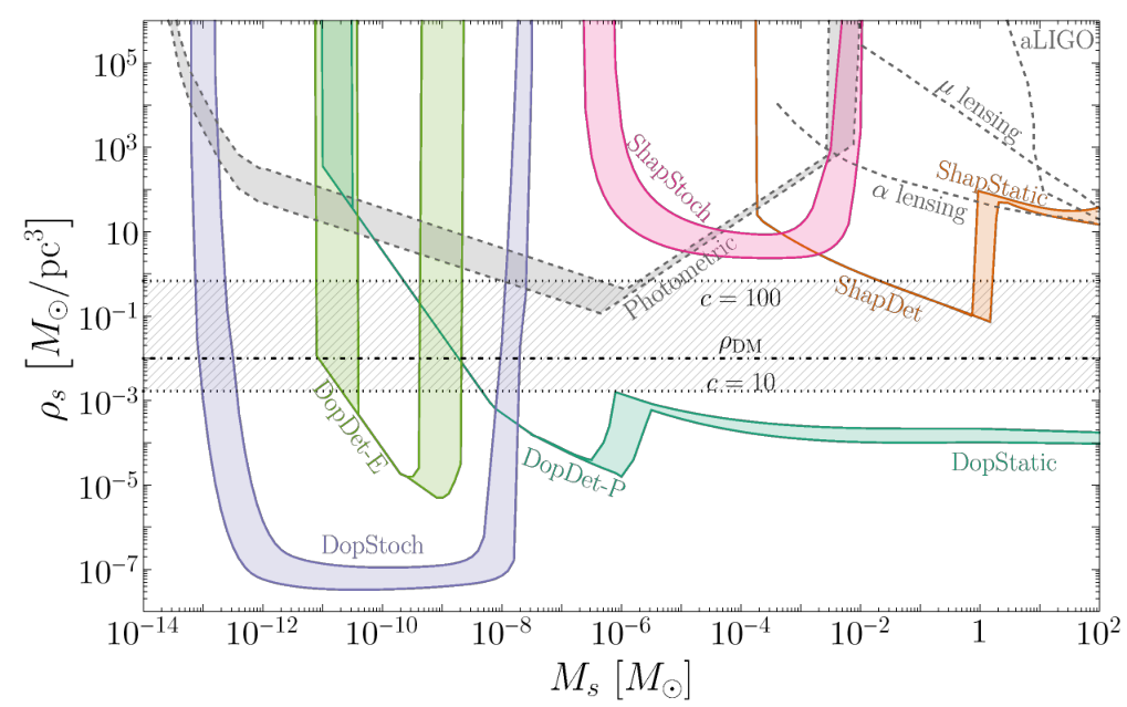
III.2 Extended Halo Mass Functions
We now consider a mass distribution that is not simply monochromatic, focusing on the highly relevant case of the Cold Dark Matter (CDM) paradigm where scale invariant perturbations are seeded by inflation. The (nearly) scale invariant nature of the perturbations fairly firmly fixes the spectrum of the Halo Mass Function (HMF), which can be parameterized as
| (59) | ||||
| (60) |
where the overall normalization, , is found by requiring that the expected matter density is equal to its measured value, . The total number of subhalos within a volume is given by,
| (61) |
One can estimate with the standard Press-Schechter theory Press and Schechter 1974, assuming a scale invariant primordial power spectrum. For large the power spectrum today scales as , up to the free-streaming scale (which sets ), corresponding to . This scale invariant spectrum gives equal mass density in equal logarithmic intervals.
Cosmological -CDM -body simulations have, however, made more precise estimates which indicate that Springel et al. 2008; Fiacconi et al. 2016. As innocent as this difference seems, it has a large impact on the constraints that can be placed at low subhalo masses where PTA constraints are most powerful. This is because, for , the mass density is dominated by the large mass subhalos. Since and are largely model-dependent, we allow them to vary, but choose parameters that do not dramatically vary from a scale invariant spectrum.
-body simulations, having dark matter only, favor constituent subhalos with an NFW profile.55 5 Baryons tend to change these profiles near the core of the subhalo, but the small subhalos that we consider here do not hold baryons Furthermore, CDM subhalos, obtained from galactic simulations Wang et al. 2019; Ludlow et al. 2014; Springel et al. 2008; Diemer and Joyce 2019, are typically quoted to have concentration parameters with for subhalos below . These models, however, are usually obtained from simulation data with . More recent simulations which study lower mass subhalos suggest that, below , the concentration parameter decreases with decreasing mass Wang et al. 2019. While the ‘Doppler-stoch’ search will have some reach for , it will only be at masses much smaller than the typical minimum mass of CDM subhalos from WIMP dark matter which have . Given the uncertainty on the concentration parameters of low mass subhalos, we show our results in Figs. (8), (9) for , and the , PBH limit for comparison.
The constraints shown in Figs. (8), (9) were derived from the monochromatic mass distribution, following Ref. Carr et al. 2017. The method advocated there re-weights the monochromatic distribution constraints shown in Fig. (2), , according to the relation
| (62) |
To check the validity of this approximation, we compare the results obtained utilizing this analytic prescription with a Monte Carlo, in Fig. (11). We see good agreement for more than one HMF, and proceed to use this analytic formula in our main results, Figs. (8), (9).
The first row in Fig. (8) shows constraints for , and the second . We take (the Milky Way galaxy mass) and to show the dependence on in the left and middle columns, and lastly , in the right column. Such narrow HMFs can be produced in theories with peaks in the primordial power spectrum Hogan and Rees 1988; Kolb and Tkachev 1993; Kolb and Tkachev 1994; Zurek et al. 2007; Buschmann et al. 2020; Arvanitaki et al. 2020; Graham et al. 2016; Erickcek and Sigurdson 2011; Barenboim and Rasero 2014; Fan et al. 2014. We will use a shorthand for the variety of search types: ‘DopDet-P+Static’ for the combined deterministic and static Doppler searches that involve the pulsar term, ‘ShapDet+Static’ for the combined deterministic and static Shapiro searches, ‘DopStoch’ for the stochastic Doppler signal, and ‘ShapStoch’ for stochastic Shapiro signal. The ‘DopDet-P+Static’ and ‘ShapDet+Static’ curves were derived in Ref. Dror et al. 2019 and corrected due to the subtraction procedure here, while ‘DopStoch’ and ‘ShapStoch’ were derived here.
It is clear from Eq. (62) that there is enhanced sensitivity to Halo Mass Functions with large support to masses for which a particular type of PTA search is sensitive. We show this in Fig. (10) by comparing PTA search constraints from Fig. (3) and the mass fraction in , , for a few different HMFs. This translates to sensitivity in Fig. (8) when and encapsulate the entire mass sensitivity range of a particular type of search. In addition, if is substantially larger than the sensitivity range of a particular search, this results in the reduction of reach to such dark matter masses; this is simply because the fraction of dark matter in the sensitivity range is diluted. Across the board, this is seen in weaker limits for compared to . However this reduction scales only as for , such that there is only a logarithmic decline for small enough in the top row, left and middle panels of Fig. (8). For , so that the reach curves flatten out for small enough in the left and middle panels.
For and with , non-trivial constraints will be set with an SKA-like PTA for and above, from the deterministic Doppler and Shapiro constraints derived in Ref. Dror et al. 2019, primarily due to the sensitivity to a wide range in mass. There is less reach for due to the skew of the HMF towards larger mass subhalos, as can be seen in Fig. (10). There are more optimistic projections when , even for small concentration parameters.

In order to demonstrate what will be necessary from PTAs to probe CDM-like substructure, we also show improvements in projected reach as some PTA parameters are dialed to more optimistic values in Fig. (9). We take the SKA-like parameters discussed in Sec. II.3 and increase the observing time to years in the left panel, the number of pulsars to in the middle panel and finally a combined set of optimistic parameters (, , , , ) in the right panel. years of observation time will allow reach to HMFs with and subhalos with via the deterministic event Doppler constraints from Ref. Dror et al. 2019. With the optimistic set of PTA parameters shown in the right-hand panel, the stochastic Doppler signal can reach subhalos with concentration parameters composing less than two percent of dark matter.
III.3 Backgrounds
Similar to direct detection of dark matter, non-observation of a signal allows one to set constraints, but a claim for discovery requires careful noise discrimination. While the noise modeling adopted in this work assumes only white noise, red-noise has been observed in some pulsars primarily due to intrinsic deviations from the spin-down timing model Wang 2015 and fluctuations in the dispersion measure Becker et al. 2018. Similar to stochastic gravitational waves, the signal can be differentiated from the background exploiting the differences in the power spectral indices Wang 2015. The contributions from the interstellar medium are dependent on the pulsar light frequency and could be corrected for without removing the pulsar-frequency-independent dark matter signal. Furthermore in the case of the Earth term, variations unique to individual pulsars are suppressed when considering cross-correlations between pulsars.
Gravitational waves from supermassive black hole merger events are expected to be detected before a dark matter signal and hence will constitute another background to a dark matter signal Lommen 2015. A single merger event can be differentiated from the deterministic dark matter subhalo event via the characteristic signal shape, as outlined in Ref. Dror et al. 2019. The stochastic gravitational wave background will also have a different power spectral index compared to the stochastic dark matter signal analyzed in this work. Furthermore, dark matter signals are dipolar in nature and exhibit characteristically different angular correlations compared to gravitational waves which are quadrupolar signal. See e.g. Ref. Jenet and Romano 2015 for the analog of the Hellings and Downs analysis Hellings and Downs 1983 for other signal patterns.
Finally, baryonic objects could cause Doppler and Shapiro delays identical to dark matter subhalos in the mass range of sensitivity. However the baryonic matter is dominated by stars in the solar mass range Fukugita and Peebles 2004, which would only affect the static signals. A discovery here would necessarily involve supplemental analysis with luminosity discrimination. At lower masses (), sub-stellar objects including brown dwarfs make up less than one percent of the total baryon density. At even lower masses, planets make up less than of all the baryons. Furthermore these objects have to be transiting and not bound to the pulsar/solar system in order to mimic a dark matter signal. Nonetheless, pulsars in baryon rich environments might very well display irreducible backgrounds from these loose baryonic objects in certain mass ranges. However, for high latitude pulsars which have been discovered recently Lorimer 2008, the baryonic background will not be limiting in the near future due to the strong limits set on by gravitational MACHO lensing surveys.
IV Conclusions
Pulsar Timing Arrays offer a unique glimpse of dark matter substructure at previously inaccessible small scales. Current constraints from measurements of large scale structure, for diffuse CDM-like subhalos, become weak below . For objects as dense as primordial black holes, observational limits from disruption of structure in conjunction with lensing extend the reach down to , though these limits are rapidly lifted as soon as the subhalos become become even modestly less dense. By contrast, the methods presented here, and in our companion paper Dror et al. 2019, reach subhalos having a concentration parameter as small as and as light as . PTAs are thus potentially more powerful than other existing or proposed probes of dark matter substructure.
As summarized in Figs. (2), (3), we showed that future PTAs will be able to place strong constraints on the fraction of dark matter in such substructure, even for NFW subhalos having a concentration as small as where lensing cannot reach. We also found that our analysis utilizing multiple transiting subhalos causing a stochastic signal can extend constraints for both Doppler and Shapiro signals by more than an order of magnitude to smaller mass relative to the constraint obtained from a deterministic event of a single transiting subhalo Dror et al. 2019, as seen by comparing the curves labeled ‘stoch’ to the other curves in Fig. (2).
A definitive goal is to observe substructure consistent with ordinary CDM at as small of a mass scale as possible, to see to what mass scale such substructures persist. For the SKA-like PTA parameters described at the end of Sec. II.3, we find this will be difficult unless the power spectrum is significantly more skewed towards low mass subhalos than we expect from standard CDM, as shown in Fig. (8). We showed the requirements from a PTA in Fig. (9) to reach standard CDM. While in principle possible, standard CDM offers a challenge, though one that would offer an unprecedented view if reached.
On the other hand, dark matter often has dynamics that, on small scales, enhance the density perturbations seeded by adiabatic, scale-invariant inflation. The formalism developed here is sufficiently general to account for any HMF. In future work we will apply this to other well motivated forms of substructure, such as axion miniclusters, cosmologies with a period of matter domination, and vector bosons produced during inflation. Observing dark matter substructure on small scales gives a unique window into post-inflationary dynamics and the nature of the dark matter.
Acknowledgements.
We thank Nikita Blinov and Jeff Dror for useful discussions, and Steve Taylor and Michele Vallisneri for discussions on the NANOGrav data and analysis. H.R. is supported in part by the DOE under contract DE-AC02-05CH11231. Some of this work was done at the Aspen Center for Physics, which is supported by NSF grant PHY-1607611 and at KITP, supported in part by the National Science Foundation under Grant No. NSF PHY-1748958. T.T. would like to thank the Walter Burke Institute for Theoretical Physics for hospitality during the completion of this work.Appendix A Derivation of the Optimal SNR
We derive the optimal signal-to-noise ratio (SNR) for different signals using a matched filter procedure, similar to Refs. Smith and Caldwell 2019; Moore et al. 2015; Allen and Romano 1999. To generalize our discussion we define the measured signal, , the dark matter signal , and the noise in the detector, , which satisfies the relation for pulsar . We will derive the optimal SNR for a deterministic signal, where is known, as well as a stochastic signal where is known. We will consider both a pulsar term, which assumes an independent signal in each pulsar, and an Earth term, where correlations between pulsars can boost the SNR. For most of the derivation we assume that the detector noise is stationary and independent across pulsars,
| (63) |
Finally we will simplify the SNR in the limit where the timing residual noise is white and identical in each pulsar: , where is the measurement cadence. The residual noise is related to the timing residual by a factor of the pulsar frequency, and therefore66 6 The signals discussed in the main text also have an accompanying factor of , and, as we will show, the SNR is independent of this factor.
| (64) | ||||
| (65) |
A.1 Deterministic Signal SNR
We begin with computing the optimal SNR for a deterministic signal. This derivation will closely follow the discussion given in Ref. Moore et al. 2015. We begin by defining a test statistic,
| (66) |
where is a filter function chosen to maximize the SNR,
| (67) |
The subscripts on indicate what is assumed to be. We can compute the expectation values,
| (68) | ||||
| (69) | ||||
| (70) |
The SNR is then,
| (71) |
The which optimizes this SNR is , and therefore the optimal SNR is
| (72) |
Assuming the noise is white and pulsar independent we can further simplify,
| (73) |
If the signal is independent in each pulsar and the SNR is dominated by the largest signal across the array, then the SNR can be approximated as
| (74) |
which we define as the pulsar term SNR. If the signal has a similar amplitude, but not independent across the pulsars, then Eq. (73) will be parametrically larger by a factor of . We define this as the Earth term SNR, because it’s the SNR used when the dark matter interacts with the Earth. We can simplify this further by replacing the sum with an average over the pulsar positions, defined by
| (75) |
A.2 Stochastic Pulsar Term SNR
We begin by defining a test statistic, ,
| (76) |
where is a filter function applied to the time series of the th pulsar. Our goal is to find the ’s which maximize the SNR,
| (77) |
where the subscripts denote the assumptions under which we should evaluate the expectation values. We have
| (78) | ||||
| (79) | ||||
| (80) |
where . Evaluating the four point function of the noise,
| (81) |
which allows us to simplify Eq. (80). The two remaining terms are identical, and the whole expression can be simplified to
| (82) |
The which maximizes the SNR is and therefore the optimal SNR is
| (83) |
We can simplify further by assuming that the signal and noise are independent of the pulsar, and that the noise is white,
| (84) |
A.3 Stochastic Earth Term SNR
The derivation of the optimal Earth term SNR is similar to the pulsar term, except the test statistic is slightly different,
| (85) |
where the sum is over pairs of pulsars. There is no subtracted piece, as there is in Eq. (76), because the second term evaluates to zero when . Computing the terms in the SNR gives,
| (86) | ||||
| (87) | ||||
| (88) |
where and we use a finite time delta function to remove the integrals. Computing the four point function, noting that , by definition gives,
| (89) |
Substituting this expression in gives two identical terms which we can simplify to
| (90) |
Again one can show that the optimal is and therefore the optimal SNR is given by
| (91) |
Lastly, we assume that the noise is white and identical across pulsars, and replace the sum by taking an average over the pulsar positions, denoted by ,
| (92) |
Appendix B Subtraction of Best Fit Parameters in PTA Signal
We discuss how the parameters of the pulsar timing model, e.g. , impacts the inferred dark matter signal. Let denote the phase that is measured at time , and therefore the goodness of fit is characterized by 77 7 In a PTA measurement, is measured at an arrival time of the th pulse such that is subtracted in the standard discrete time formulation of . The analysis here only differs by working in continuous time.
| (93) |
The generalization to a timing model with higher order terms is straightforward. In order to find the best-fit parameters we minimize with respect to , which is more easily done by defining an inner product,
| (94) |
along with a set of polynomial basis functions, , with respect to this inner product, 88 8 These are related to the standard Legendre polynomials, , by a scaling and shift: .
| (95) |
Therefore in Eq. (93) can be written as
| (96) |
where . We can now minimize with respect to (and later work out if necessary). The minimization condition is
| (97) |
and therefore . The residual, , is then given by , and the subtracted DM signal, , is related to the unsubtracted signal, by,
| (98) |
This is how the subtraction procedure effects the single deterministic event analysis, as the SNR is only a function of . However for the stochastic signal the subtraction procedure enters through a correlator of subtracted signals. We can relate the unsubtracted correlator, , to the subtracted correlator, , by
| (99) |
where
| (100) | ||||
| (101) |
The results of this procedure are quoted in Eq. (30). The effect of this subtraction procedure on the reach to monochromatic PBHs can be seen in Fig. (12). Note that in this figure we have not included ‘Static’ constraints, as these are derived with only and higher order terms, such that subtraction cannot be meaningfully applied to this analysis.
Appendix C Relationship with the Power Spectrum Approach
In this section, we explain the difference between this work and the power spectrum procedure adopted in Ref. Baghram et al. 2011. If the observing volume is all of space then in Eq. (14), for the Doppler and Shapiro delays, can be written in terms of the matter power spectrum, as done in Ref. Baghram et al. 2011.99 9 The signal correlator we consider here and considered in Ref. Baghram et al. 2011 are related by . To show this, we simplify the gravitational potential correlator, from which both the Doppler and Shapiro signal correlators can be derived. For example, the Shapiro delay frequency shift correlator is
| (102) |
where is the Fourier transform of the gravitational potential at position , and represents all of the random variables, etc.
Since the object’s individual potentials only depend on the distance from the center of mass, ,
| (103) |
The potential correlator is then a sum over individual contributions as,
| (104) |
where the subscripted denotes averaging over only the subscripted random variable. In the limit where the integral is over all space, the exponential in the term becomes a delta function, and the potential correlator from a single subhalo can be simplified,
| (105) | ||||
| (106) |
where is the 1-subhalo matter power spectrum. It can be shown that the term in Eq. (104) simplifies similarly with being replaced by . Finally,
| (107) |
and the rest of the derivation for the signal correlator proceeds as in Ref. Baghram et al. 2011. However the Earth-pulsar system samples a finite volume of space, since subhalos at a larger distance are static, and hence susceptible to being absorbed in the fit. To obtain a physical result from a power spectrum approach one would need to introduce cuts on the integral to incorporate these finite volume effects. Here we simplify the signal correlators differently than Ref. Baghram et al. 2011 by incorporating finite volume effects directly in the subhalo position average.
Appendix D Form Factor Integral
We derive an analytic expression for the form factor in Eq. (18),
| (108) |
with the definition of ,
| (109) |
Substituting this in to Eq. (108),
| (110) |
and using
| (111) |
gives
| (112) |
Assuming is given by an NFW profile then
| (113) | ||||
| (114) |
and therefore
| (115) |
We can simplify further by changing variables. Defining , and
| (116) |
We see that the form factor is only a function of and , as shown in Fig. 6.
References
- Green et al. (2005) A. M. Green, S. Hofmann, and D. J. Schwarz, JCAP 0508, 003 (2005), arXiv:astro-ph/0503387 [astro-ph] .
- Hogan and Rees (1988) C. Hogan and M. Rees, Physics Letters B 205, 228 (1988).
- Kolb and Tkachev (1993) E. W. Kolb and I. I. Tkachev, Phys. Rev. Lett. 71, 3051 (1993), arXiv:hep-ph/9303313 [hep-ph] .
- Kolb and Tkachev (1994) E. W. Kolb and I. I. Tkachev, Phys. Rev. D49, 5040 (1994), arXiv:astro-ph/9311037 [astro-ph] .
- Zurek et al. (2007) K. M. Zurek, C. J. Hogan, and T. R. Quinn, Phys. Rev. D75, 043511 (2007), arXiv:astro-ph/0607341 [astro-ph] .
- Buschmann et al. (2020) M. Buschmann, J. W. Foster, and B. R. Safdi, Phys. Rev. Lett. 124, 161103 (2020), arXiv:1906.00967 [astro-ph.CO] .
- Arvanitaki et al. (2020) A. Arvanitaki, S. Dimopoulos, M. Galanis, L. Lehner, J. O. Thompson, and K. Van Tilburg, Phys. Rev. D 101, 083014 (2020), arXiv:1909.11665 [astro-ph.CO] .
- Graham et al. (2016) P. W. Graham, J. Mardon, and S. Rajendran, Phys. Rev. D93, 103520 (2016), arXiv:1504.02102 [hep-ph] .
- Erickcek and Sigurdson (2011) A. L. Erickcek and K. Sigurdson, Phys. Rev. D84, 083503 (2011), arXiv:1106.0536 [astro-ph.CO] .
- Barenboim and Rasero (2014) G. Barenboim and J. Rasero, JHEP 04, 138 (2014), arXiv:1311.4034 [hep-ph] .
- Fan et al. (2014) J. Fan, O. Özsoy, and S. Watson, Phys. Rev. D90, 043536 (2014), arXiv:1405.7373 [hep-ph] .
- Blinov et al. (2020) N. Blinov, M. J. Dolan, and P. Draper, Phys. Rev. D 101, 035002 (2020), arXiv:1911.07853 [astro-ph.CO] .
- Gilman et al. (2020) D. Gilman, S. Birrer, A. Nierenberg, T. Treu, X. Du, and A. Benson, Mon. Not. Roy. Astron. Soc. 491, 6077 (2020), arXiv:1908.06983 [astro-ph.CO] .
- Bonaca et al. (2019) A. Bonaca, D. W. Hogg, A. M. Price-Whelan, and C. Conroy, The Astrophysical Journal 880, 38 (2019).
- Muñoz et al. (2020) J. B. Muñoz, C. Dvorkin, and F.-Y. Cyr-Racine, Phys. Rev. D 101, 063526 (2020), arXiv:1911.11144 [astro-ph.CO] .
- Diaz Rivero et al. (2018) A. Diaz Rivero, F.-Y. Cyr-Racine, and C. Dvorkin, Phys. Rev. D97, 023001 (2018), arXiv:1707.04590 [astro-ph.CO] .
- Buschmann et al. (2018) M. Buschmann, J. Kopp, B. R. Safdi, and C.-L. Wu, Phys. Rev. Lett. 120, 211101 (2018), arXiv:1711.03554 [astro-ph.GA] .
- Van Tilburg et al. (2018) K. Van Tilburg, A.-M. Taki, and N. Weiner, JCAP 1807, 041 (2018), arXiv:1804.01991 [astro-ph.CO] .
- Mondino et al. (2020) C. Mondino, A.-M. Taki, K. Van Tilburg, and N. Weiner, (2020), arXiv:2002.01938 [astro-ph.CO] .
- Mishra-Sharma et al. (2020) S. Mishra-Sharma, K. Van Tilburg, and N. Weiner, (2020), arXiv:2003.02264 [astro-ph.CO] .
- Brandt (2016) T. D. Brandt, Astrophys. J. 824, L31 (2016), arXiv:1605.03665 [astro-ph.GA] .
- Allsman et al. (2001) R. A. Allsman et al. (Macho), The Astrophysical Journal 550, L169 (2001), arXiv:astro-ph/0011506 [astro-ph] .
- Tisserand et al. (2007) P. Tisserand et al. (EROS-2), Astronomy & Astrophysics 469, 387 (2007), arXiv:astro-ph/0607207 [astro-ph] .
- Wyrzykowski et al. (2011) L. Wyrzykowski et al., Monthly Notices of the Royal Astronomical Society 416, 2949 (2011), arXiv:1106.2925 [astro-ph.GA] .
- Niikura et al. (2019) H. Niikura, M. Takada, N. Yasuda, R. H. Lupton, T. Sumi, S. More, A. More, M. Oguri, and M. Chiba, Nature Astronomy 3, 524 (2019), arXiv:1701.02151 [astro-ph.CO] .
- Smyth et al. (2019) N. Smyth, S. Profumo, S. English, T. Jeltema, K. McKinnon, and P. Guhathakurta, (2019), arXiv:1910.01285 [astro-ph.CO] .
- Griest et al. (2014) K. Griest, A. M. Cieplak, and M. J. Lehner, Astrophys. J. 786, 158 (2014), arXiv:1307.5798 [astro-ph.CO] .
- Katz et al. (2018) A. Katz, J. Kopp, S. Sibiryakov, and W. Xue, JCAP 1812, 005 (2018), arXiv:1807.11495 [astro-ph.CO] .
- Katz et al. (2019) A. Katz, J. Kopp, S. Sibiryakov, and W. Xue, (2019), arXiv:1912.07620 [astro-ph.CO] .
- Dror et al. (2019) J. A. Dror, H. Ramani, T. Trickle, and K. M. Zurek, Phys. Rev. D100, 023003 (2019), arXiv:1901.04490 [astro-ph.CO] .
- Croon et al. (2020) D. Croon, D. McKeen, and N. Raj, Phys. Rev. D 101, 083013 (2020), arXiv:2002.08962 [astro-ph.CO] .
- Dai and Miralda-Escudé (2020) L. Dai and J. Miralda-Escudé, Astron. J. 159, 49 (2020), arXiv:1908.01773 [astro-ph.CO] .
- Siegel et al. (2007a) E. R. Siegel, M. Hertzberg, and J. Fry, Mon. Not. Roy. Astron. Soc. 382, 879 (2007a), arXiv:astro-ph/0702546 .
- Seto and Cooray (2007a) N. Seto and A. Cooray, Astrophys. J. 659, L33 (2007a), arXiv:astro-ph/0702586 .
- Clark et al. (2016) H. A. Clark, G. F. Lewis, and P. Scott, Mon. Not. Roy. Astron. Soc. 456, 1394 (2016), [Erratum: Mon.Not.Roy.Astron.Soc. 464, 2468 (2017)], arXiv:1509.02938 [astro-ph.CO] .
- Schutz and Liu (2017) K. Schutz and A. Liu, Phys. Rev. D 95, 023002 (2017), arXiv:1610.04234 [astro-ph.CO] .
- Baghram et al. (2011) S. Baghram, N. Afshordi, and K. M. Zurek, Phys. Rev. D84, 043511 (2011), arXiv:1101.5487 [astro-ph.CO] .
- Kashiyama and Seto (2012) K. Kashiyama and N. Seto, MNRAS 426, 1369 (2012), arXiv:1208.4101 .
- Kashiyama and Oguri (2018) K. Kashiyama and M. Oguri, (2018), arXiv:1801.07847 [astro-ph.CO] .
- Rosado et al. (2015) P. A. Rosado, A. Sesana, and J. Gair, Mon. Not. Roy. Astron. Soc. 451, 2417 (2015), arXiv:1503.04803 [astro-ph.HE] .
- Siegel et al. (2007b) E. R. Siegel, M. P. Hertzberg, and J. N. Fry, Monthly Notices of the Royal Astronomical Society 382, 879 (2007b), arXiv:astro-ph/0702546 [astro-ph] .
- Seto and Cooray (2007b) N. Seto and A. Cooray, Astrophys. J. 659, L33 (2007b), arXiv:astro-ph/0702586 [astro-ph] .
- Moore et al. (2015) C. J. Moore, R. H. Cole, and C. P. L. Berry, Class. Quant. Grav. 32, 015014 (2015), arXiv:1408.0740 [gr-qc] .
- Smith and Caldwell (2019) T. L. Smith and R. Caldwell, Phys. Rev. D 100, 104055 (2019) (2019), 10.5281/zenodo.3341817, arXiv:1908.00546v1 [astro-ph.CO] .
- Desvignes et al. (2016) G. Desvignes et al., Mon. Not. Roy. Astron. Soc. 458, 3341 (2016), arXiv:1602.08511 [astro-ph.HE] .
- Manchester et al. (2013) R. N. Manchester et al., Publ. Astron. Soc. Austral. 30, 17 (2013), arXiv:1210.6130 [astro-ph.IM] .
- Arzoumanian et al. (2016) Z. Arzoumanian et al. (NANOGrav), Astrophys. J. 821, 13 (2016), arXiv:1508.03024 [astro-ph.GA] .
- Bailes et al. (2018) M. Bailes et al., Proceedings, MeerKAT Science: On the Pathway to the SKA (MeerKAT2016): Stellenbosch, South Africa, May 25-27, 2016, PoS MeerKAT2016, 011 (2018), arXiv:1803.07424 [astro-ph.IM] .
- Hobbs et al. (2019) G. Hobbs, S. Dai, R. N. Manchester, R. M. Shannon, M. Kerr, K. J. Lee, and R. Xu, Res. Astron. Astrophys. 19, 020 (2019), arXiv:1407.0435 [astro-ph.IM] .
- Perera et al. (2019) B. B. P. Perera et al., Mon. Not. Roy. Astron. Soc. 490, 4666 (2019), arXiv:1909.04534 [astro-ph.HE] .
- Reardon et al. (2016) D. Reardon, G. Hobbs, W. Coles, Y. Levin, M. Keith, M. Bailes, N. Bhat, S. Burke-Spolaor, S. Dai, M. Kerr, et al., Monthly Notices of the Royal Astronomical Society 455, 1751 (2016).
- Arzoumanian et al. (2015) Z. Arzoumanian et al. (NANOGrav), Astrophys. J. 813, 65 (2015), arXiv:1505.07540 [astro-ph.IM] .
- Zumalacárregui and Seljak (2018) M. Zumalacárregui and U. Seljak, Physical Review Letters 121 (2018), 10.1103/physrevlett.121.141101.
- Laha et al. (2020) R. Laha, J. B. Muñoz, and T. R. Slatyer, (2020), arXiv:2004.00627 [astro-ph.CO] .
- Van Haasteren and Levin (2018) R. Van Haasteren and Y. Levin, Mon. Not. R. Astron. Soc, Tech. Rep. 0000 (2018) arXiv:0909.0954v1 .
- Dai et al. (2018) L. Dai, S.-S. Li, B. Zackay, S. Mao, and Y. Lu, Phys. Rev. D 98, 104029 (2018), arXiv:1810.00003 [gr-qc] .
- Moline et al. (2017) A. Moline, M. A. Sanchez-Conde, S. Palomares-Ruiz, and F. Prada, Mon. Not. Roy. Astron. Soc. 466, 4974 (2017), arXiv:1603.04057 [astro-ph.CO] .
- Wang et al. (2019) J. Wang, S. Bose, C. S. Frenk, L. Gao, A. Jenkins, V. Springel, and S. D. M. White, (2019), arXiv:1911.09720 [astro-ph.CO] .
- Press and Schechter (1974) W. H. Press and P. Schechter, Astrophys. J. 187, 425 (1974).
- Springel et al. (2008) V. Springel, J. Wang, M. Vogelsberger, A. Ludlow, A. Jenkins, A. Helmi, J. F. Navarro, C. S. Frenk, and S. D. M. White, Mon. Not. Roy. Astron. Soc. 391, 1685 (2008), arXiv:0809.0898 [astro-ph] .
- Fiacconi et al. (2016) D. Fiacconi, P. Madau, D. Potter, and J. Stadel, Astrophys. J. 824, 144 (2016), arXiv:1602.03526 [astro-ph.GA] .
- Ludlow et al. (2014) A. D. Ludlow, J. F. Navarro, R. E. Angulo, M. Boylan-Kolchin, V. Springel, C. Frenk, and S. D. M. White, Mon. Not. Roy. Astron. Soc. 441, 378 (2014), arXiv:1312.0945 [astro-ph.CO] .
- Diemer and Joyce (2019) B. Diemer and M. Joyce, Astrophys. J. 871, 168 (2019), arXiv:1809.07326 [astro-ph.CO] .
- Carr et al. (2017) B. Carr, M. Raidal, T. Tenkanen, V. Vaskonen, and H. Veermäe, Phys. Rev. D96, 023514 (2017), arXiv:1705.05567 [astro-ph.CO] .
- Wang (2015) Y. Wang, J. Phys. Conf. Ser. 610, 012019 (2015), arXiv:1505.00402 [astro-ph.IM] .
- Becker et al. (2018) W. Becker, M. Kramer, and A. Sesana, Space Sci. Rev. 214, 30 (2018), arXiv:1705.11022 [astro-ph.IM] .
- Lommen (2015) A. N. Lommen, Reports on Progress in Physics 78, 124901 (2015).
- Jenet and Romano (2015) F. A. Jenet and J. D. Romano, Am. J. Phys. 83, 635 (2015), arXiv:1412.1142 [gr-qc] .
- Hellings and Downs (1983) R. Hellings and G. Downs, Astrophys. J. 265, L39 (1983).
- Fukugita and Peebles (2004) M. Fukugita and P. E. Peebles, Astrophys. J. 616, 643 (2004), arXiv:astro-ph/0406095 .
- Lorimer (2008) D. R. Lorimer, Living reviews in relativity 11, 8 (2008).
- Allen and Romano (1999) B. Allen and J. D. Romano, Physical Review D 59 (1999), 10.1103/physrevd.59.102001.