Interface-resolved simulation of the evaporation and combustion of a fuel droplet suspended in normal gravityJournal: Fuel
Abstract
An interface-resolved simulation of the combustion of a fuel droplet suspended in normal gravity is presented in this work, followed by an extensive analysis on the physical aspects involved. The modeling is based on DropletSMOKE++, a multiphase solver developed for the modeling of droplet vaporization and combustion in convective conditions. A wide range of phenomena can be described by the model, including the interface advection, the phase-change, the combustion chemistry, non-ideal thermodynamics and multicomponent mixtures. To our knowledge, this is the most detailed simulation performed on this configuration, providing a useful theoretical and numerical support for the experimental activity on this field. A recent experimental work is used as a reference, in which a methanol droplet is suspended on a quartz fiber and ignited at different oxygen concentrations. The numerical analysis offers a detailed insight into the physics of the problem and a satisfactory agreement with the experiments in terms of diameter decay, radial temperature profiles and sensitivity to the oxygen concentration. The vaporization rate is affected by the thermal conduction from the fiber, due to the high temperatures involved. Moreover, the fiber perturbs the flame itself, providing quenching at its surface. The combustion physics is compared to the one predicted at zero-gravity, evidencing a lower standoff-ratio, a higher flame temperature and an intense internal circulation. The distribution of the species around the droplet shows (i) a local accumulation of intermediate oxidation products at the fiber surface and (ii) water absorption in the liquid phase, affecting the vaporization rate.
Keywords:
droplet combustion , evaporation , flame , VOF , support fiber , methanolNomenclature
- Acronyms
[VOF]Volume Of Fluid
- Greek letters
-
VOF marker function
-
scalar dissipation rate
-
enthalpy of reaction
-
evaporation enthalpy
-
Dirac delta
-
activity coefficient
-
mixture gas-phase fugacity coefficient
-
curvature
-
dynamic viscosity
-
stoichiometric coefficient
-
mass fraction
-
pure gas-phase fugacity coefficient
-
generic variable
-
density
-
surface tension
- Roman letters
-
evaporation flux
-
heat flux per unit volume
-
mass diffusion coefficient
- f
force per unit volume
- j
diffusion flux
- v
velocity
- x
position vector
-
absorption coefficient
-
constant pressure specific heat
-
diameter
-
height of the mesh
-
thermal conductivity
-
base radius of the mesh
-
molecular weight
-
Number of species
-
pressure
-
vapor pressure
-
dynamic pressure
-
reaction rate
-
radius
-
time
-
temperature
-
molar volume
-
mole fraction
-
mixture fraction
- Superscripts and subscripts
-
initial, reference
-
boiling
-
ambient
-
fiber
-
gas
-
-th species
-
-th reaction
-
liquid
-
radiative
-
solid
1 Introduction
Spray and droplet combustion technologies are adopted in a wide range of practical applications: power generation, propulsion, fuel injectors etc. The numerical simulation of burning sprays is rapidly advancing, but major difficulties remain due to the inherent complexity of the problem: breakups, coalescence phenomena, surface tension instabilities, interactions with a turbulent gas flow are very complex phenomena, not yet fully understood tryggvason2011direct. Phase-change and gas-phase combustion further complicate the problem, while the wide range of spatial scales involved (several orders of magnitude), makes the numerical modeling extremely expensive in terms of computational resources. Hence, the need of simplified but still physically representative configurations: in this context, the study of the evaporation and combustion of a single isolated droplet represents an essential step towards the better understanding of a complex system like a spray.
The research on isolated droplets has been of interest for nearly 70 years, as testified by the numerous theoretical and experimental works in the field faeth1979current, law1982recent, helenbrook2002quasi, okajima1975further, dietrich1996droplet, cuoci2005autoignition, farouk2014isolated, cuoci2017flame, morin2004vaporization, birouk2000turbulence, chauveau2019analysis, avedisian1988low, yang1991combustion, jackson1991soot, liu2016comprehensive, xu2017combustion. These works are typically based on relatively large droplets ( mm) if compared to the ones generated by a spray atomizer ( m). This aspect is often adopted to question on the relevance of single droplet investigations for practical applications. It is worth pointing out the importance of studying isolated droplets, which is very relevant for different reasons:
- 1.
It allows to isolate and focus on the phase-change and reactive processes, decoupling them from the interactions typically involved in a spray such as breakups, coalescence and fragmentation. It also serves as a simplified/ideal system to investigate the sensitivity and quality of the sub-models included in the numerical description (e.g. kinetic mechanism, species mass diffusion etc.);
- 2.
It provides a basis for refining the understanding of vaporization, ignition and extinction processes and allows to quantitatively assess the capability to predict these phenomena and their mutual interaction (e.g. the diffusion-reaction interaction, the effect of buoyancy on evaporation, the role of radiation on flame extinction, the effect of convection on the ignition properties etc.);
- 3.
Sprays are commonly treated as a collection of zero-dimensional points tracked in a Lagrangian way, adopting a RANS/LES approach for turbulence modeling. The coupling between the flow and the particles requires additional subgrid scale models for the droplet source terms (e.g. heat and mass transfer rates) and for the particle-flow interaction (e.g. drag force). These closure models need to be developed and validated based on the detailed analysis of simpler configurations, such as single droplets helenbrook2002quasi.
It is clear, however, that the first step is the development of dedicated numerical simulations, at a level of detail necessary to describe of the physico-chemical phenomena involved in droplet combustion. In the last decades, researchers mainly focused on a simple, idealized condition in which a spherical droplet was investigated in microgravity okajima1975further, dietrich1996droplet, because of the absence of buoyancy effects and droplet deformation. This was also attractive for the relatively simple mathematical modeling, exploiting the spherical symmetry of the system and leaving room for a more detailed chemistry description cuoci2005autoignition, farouk2014isolated, cuoci2017flame. However, even if the microgravity condition still represents a valuable method for droplets analysis, there is a strong interest in considering more realistic situations in which convection and gravity play a significant role (like in sprays). The most common case is represented by the vaporization, ignition and combustion of a single droplet suspended in normal gravity, for which a very large number of experimental works is available morin2004vaporization, birouk2000turbulence, chauveau2019analysis, pfeil2013effects, chauveau2000effects, chauveau1999effects, shaw2012combustion. Despite the amount of experiments on convective droplet combustion, the attempts to model these systems are scarce.
The main reason lies in the high complexity of the mathematical description, which requires a CFD multiphase model that incorporates: (i) a numerical method for the interface advection, (ii) the solution of a two-phase velocity field, (iii) a resolved-boundary layer model for evaluating the vaporization rate in convective conditions, (iv) a multi-region approach to model the flame-fiber thermal interaction chauveau2008experimental and (v) the implementation of gas-phase combustion. Some noteworthy papers can be found for pure evaporation in normal gravity george2017detailed, wang2019vaporization, but very few numerical works on combustion are available and mainly limited to non-shrinking, motionless droplets wang2018fully or adopting one-step/global schemes for chemistry jin2010computational. Only recently a skeletal mechanism (20 reactions) was used by Ghata et al. ghata2015computational within a multiphase approach, limiting however the application to microgravity conditions.
This work presents a full interface-resolved numerical simulation of the vaporization and combustion of a suspended fuel droplet in normal gravity and demonstrates the potential of this approach in unraveling several physical phenomena not obtainable otherwise. The recent experimental work of Yadav et al. yadav2017interferometric has been adopted as a reference case for the detailed analysis of convective droplet combustion: a methanol droplet is suspended on a quartz vertical fiber (at ambient temperature and pressure) and ignited with a spark, tracking the combustion phenomena and the droplet characteristics over time.
The numerical modeling is based on the DropletSMOKE++ solver saufi2019dropletsmoke++, saufi2019experimental, a CFD code conceived for the vaporization and combustion modeling of fuel droplets (including i, ii, iii, iv, v). The analysis of the numerical simulation allows to get a very detailed insight into the physics of the problem, which is the main objective of this work. The paper organization reflects this purpose, including: a description of the main mathematical model (Section 3), the numerical methodology (Section 4), the numerical modeling of the experiments and the extended analysis on the main physical peculiarities of the system (Section 5), such as the flame-fiber interaction, the effect of gravity on the flame properties, the main species distribution around the droplet and the impact of water absorption in the liquid phase. The paper finishes with the conclusions.
2 Experimental setup
The experiments are carried out in a closed combustion chamber (70x70x100 mm3) in which a methanol droplet ( mm) is suspended with a syringe on a quartz vertical fiber ( mm) at 300 K and atmospheric pressure. The chamber is much larger than the maximum droplet diameter ( 50) to avoid significant changes in the boundary conditions due to oxygen depletion. Two steel electrodes (attached to a 14.5 kV ignition transformer) initiate the combustion, which is followed in two ways: a digital camera (60 fps) tracks the droplet surface regression, while a Mach Zehnder interferometer provides the whole temperature field distribution in a non-intrusive manner. More specific details (not necessary for the present modeling work) can be found in the reference work yadav2017interferometric.
3 Mathematical model
DropletSMOKE++ is a multiphase CFD code based on the Volume Of Fluid (VOF) methodology for the interface advection. In addition to the governing equations enforcing the conservation of momentum, energy and species mass, a detailed description of the interface thermodynamics is implemented (based on cubic Equations of State). The evaporation rate is directly calculated from the gas-phase boundary layer and a multiregion approach for the thermal perturbation of the fiber on the droplet is included.
3.1 Interface advection
The VOF methodology hirt1981volume is an interface capturing method within an Eulerian formulation, adopting a marker function to represent the fluid phases. The marker function represents the liquid volumetric fraction, assuming value 0 in the gas-phase and value 1 in the liquid phase. The following equation for is solved:
| (1) |
where the source terms represent the contribution of the evaporation/condensation rate (depending on the sign of ) and the droplet dilation due to the change of density . The interface is advected using the isoAdvector library roenby2016computational developed by Roenby and Jasak, reconstructing the interface with a geometrical methodology. As shown in the reference paper, the isoAdvector is based on the usage of efficient isosurface calculations to estimate the distribution of fluids inside computational cells and its performances are superior to the semi-empirical compressive scheme commonly adopted in greenshields2015openfoam in terms of shape preservation, volume conservation, interface sharpness and efficiency.
3.2 Governing equations
The velocity field is shared between the two phases, solving a single Navier-Stokes equation in the whole computational domain:
| (2) |
where is the dynamic pressure, which greatly simplifies the definition of boundary conditions. The momentum equation is coupled with the following continuity equation:
| (3) |
in which the term provides the interfacial velocity jump due to the phase-change (i.e. Stefan flow). Additionally, the energy equation is included:
| (4) |
The term accounts for the interface cooling due to the evaporation of the liquid species, while the term represents the energy source due to the combustion reactions. describes the radiative heat transfer contribution. are the diffusion fluxes based on the species mole fractions gradient bird2002transport:
| (5) |
The transport equations for the species in the gas phase are:
| (6) |
where the species source term is due to the combustion reactions. represent the stoichiometric coefficient of the -th species in the -th reaction. Finally, the liquid species transport is needed for multicomponent liquids. The only difference is that a source term has to be explicitly included to account for the amount of species lost at the liquid interface for evaporation () or added by condensation ():
| (7) |
Liquid-phase reactions are not considered. Equation 7 will be adopted when dealing with water condensation on the surface (Section 5.7).
3.3 Interface thermodynamics
At the interface, vapor-liquid equilibrium conditions are assumed. Adopting a cubic Equation of State, the general equation for a two-phase systems is smithintroduction:
| (8) |
where is the vapor pressure of species , is the gas-phase fugacity coefficient for the pure species and is the gas-phase mixture fugacity coefficient. The exponential term represents the Poynting correction, while is the activity coefficient for non-ideal mixtures. For fuels burning at atmospheric pressure, the equation can be well approximated with a modified Raoult’s law:
| (9) |
The equilibrium gaseous mole fraction is evaluated explicitly:
| (10) |
as well as the equilibrium gaseous mass fraction :
| (11) |
and assigned to the whole liquid phase. Equation 6 is then solved to advect the gaseous species.
3.4 Evaporation rate
The vaporization flux of each liquid species is directly calculated from a species mass balance at the interface, imposing the gas and liquid fluxes (sum of diffusive and convective) to be equal at the interface:
| (12) |
where applies the evaporation flux only at the interface and accounts only for the normal component of . For monocomponent liquids, and . Therefore:
| (13) |
Equation 13 can be re-arranged to give the total evaporation rate reutzsch2020consistent:
| (14) |
which is equal to for monocomponent fuels. If the dot product is negative we have evaporation (), otherwise we have condensation (). Summing over the liquid species on both sides of Equation 12, the total evaporation rate for multicomponent fuels is easily obtained:
| (15) |
The total evaporation flux is used as a source term in Equation 1. The evaporation flux of each species (only needed for multicomponent cases) can be calculated using either sides of Equation 12 once is known. We use the gas-phase side:
| (16) |
3.5 Droplet suspension
In normal gravity evaporation experiments, the surface tension force suspends the liquid droplet against gravity:
| (17) |
where is the interface curvature and is a Dirac delta applied on the interface. Modeling surface tension is one of the main challenges in multiphase flows at small scales (mm and below), for two main reasons:
- 1.
The surface tension force is only applied at the interface and this makes its numerical discretization very difficult (i.e. the Dirac delta ). Standard or trivial discretization methods are not able to perfectly balance the pressure gradient and the surface tension force, developing artificial velocity spikes at the interface (called spurious currents), which can eventually grow and break the droplet apart;
- 2.
Within a VOF approach the interface curvature is not easily accessible, due to the discontinuous nature of the marker :
(18) which makes the interface normal n calculation very difficult. Numerical errors on represents another source of spurious currents, in addition to incorrect interface discretizations.
These issue is very well known in literature brackbill1992continuum, popinet2009accurate: available solutions either rely on simple filtering of the function raeini2012modelling or more rigorous methods both for the surface tension discretization (e.g. Ghost Fluid Method vukvcevic2017implementation) and curvature computation (e.g. Height Functions popinet2009accurate). While filtering techniques are proved to be non-consistent popinet2018numerical and hardly generalizable, rigorous techniques require a great effort to be correctly implemented. In particular, the framework lacks of reliable models for surface tension driven flows and no valid and general solution has been proposed so far. Moreover, the aforementioned methods are not proved to efficiently work in evaporative conditions: the presence of evaporation further worsens the problem, since the Stefan flow tends to destabilize the interface thickness. The research in this sense is still at the beginning and only few results are available palmore2019volume.
In order to overcome this problem, a centripetal force directed towards the droplet center is introduced, in order to keep the droplet attached to the fiber and suspended in the presence of a gravity field. In this way the surface tension force is not needed anymore and it can be suppressed, eliminating parasitic currents directly from their source. The Navier-Stokes equation becomes:
| (19) |
This methodology allows to model the droplet evaporation process whatever the droplet size, without worrying about the detrimental effect of spurious currents. More details about the implementation can be found in the DropletSMOKE++ reference work saufi2019dropletsmoke++.
3.6 Multiregion approach for conjugate heat transfer
The fuel droplet is suspended on a vertical fiber and evaporated under a normal gravity field. Numerous experimental and numerical analyses yang2001discrepancies, chauveau2019analysis, liu2015effect, avedisian2000soot showed that the tethering system can significantly affect the vaporization process from a thermal point of view. The solid is heated by the gaseous environment and conducts heat towards the droplet, providing a preferential path for the heat flux on the liquid. This phenomenon becomes extremely important in combustion processes (due to the high gas temperature) and when adopting large fiber diameters (due to the larger surface available for the heat transfer). The DropletSMOKE++ code includes a multiregion approach to account for the fiber thermal perturbation, firstly presented in saufi2019experimental. The heat transfer is modeled considering the real geometry of the fiber, with no need of semi-empirical correlations or approximate approaches to account for the tethering system. The fluid and the solid regions are independently meshed, solved and connected with dynamic boundary conditions, providing a full detailed numerical simulation of the three-phase system. The following equation is solved for the solid phase:
| (20) |
while the fluid temperature field is provided by Equation 4 and is the radiative heat flux from the fiber. The external surface of the solid fiber is the contact boundary between the phases. The boundary conditions describe the conservation of heat fluxes across the boundary as well as the continuity of temperature.
3.7 Gas, liquid and solid properties
The fluid properties are computed with the OpenSMOKE++ library cuoci2015opensmoke++. In particular, the gas physical properties () are based on the kinetic theory of gases, while liquid (, , ) and solid () properties are evaluated based on the correlations available in the Yaws yaws2015yaws database. The activity coefficient for non-ideal mixtures is calculated based on the UNIFAC approach fredenslund1975group. Within a VOF approach, the mixture properties to be used in the governing equations are computed as follows (e.g. for density ):
| (21) |
3.8 Combustion modeling
The DropletSMOKE++ code has been extensively validated for evaporation cases against numerous experimental data saufi2019dropletsmoke++, saufi2019experimental in a wide range of operating conditions, both in natural and forced convection. In this work, the model is extended to include the gas-phase combustion and related phenomena. In particular:
- 1.
In order to overcome the stiffness of reacting processes, the gas-phase chemistry implementation is based on an operator-splitting approach strang1968construction, separating transport and reaction terms within the same time step. The methodology is well established and in this work we adopt the specific implementation from Cuoci et al. cuoci2013computational included in the laminarSMOKE++ solver for the modeling of laminar flames with very detailed kinetic mechanisms (hundreds of species and thousands of species). In particular, the reaction step is based on the OpenSMOKE++ library cuoci2015opensmoke++, specifically developed to efficiently solve stiff ODE systems and manage detailed kinetic mechanisms. It is important to specify that reactions only occur in the gas-phase: within a VOF approach this requires the resolution of the reactive step only if in the computational cell of interest;
- 2.
An optically thin model is used for radiative heat transfer, considering H2O, CO, CO2 and CH4 as main radiating species. This is justified by the small optical depth of the system (, where is the maximum local average absorptivity and the maximum length in the domain). Planck absorption coefficients are calculated for each species and averaged based on the species mole fractions to obtain :
(22) where are the number of radiating species. Radiation is included in the temperature equation as the divergence of the radiating flux:
(23) where is the Stefan-Boltzmann constant and K. Radiation from the solid fiber is also considered in Equation 20, with for quartz yaws2015yaws:
(24) also incorporates sophisticated models for radiative heat transfer, such as P1 and DOM greenshields2015openfoam. We did not notice any significant difference for the case examined in this work (), but, if needed, their application to more geometrically complex configurations would be immediate;
- 3.
When a droplet evaporates in a mildly-hot (few hundreds degrees K) environment, the liquid surface reaches (after a transient period) a steady wet-bulb temperature, below the liquid boiling point , due to the balance of the incoming heat flux and vaporization enthalpy (Equation 4). The internal liquid temperature is generally lower. The evaporation rate in these conditions is governed by the species diffusion flux from the surface (Equations 14, 15). On the other hand, the presence of a significant thermal perturbation from the fiber (typical case in combustion processes, with tens of hundreds degrees K in the gas-phase) can push the internal liquid temperature towards the boiling point . In this case the liquid temperature profile should reach and instantaneously flatten, remaining constant.
However, Equation 4 cannot predict this profile discontinuity inside the liquid phase (the cooling term is zero outside the interface) and the internal droplet temperature would continue to increase above . In fact, the heat flux per unit volume acting on a point in the droplet is entirely used to vaporize the liquid, maintaining the local temperature constant. Therefore, the vaporization rate in the liquid phase should be calculated as:
(25) where is the vaporization enthalpy. Equation 25 is to be applied at every point in the liquid phase in which , avoiding over-heating. If the liquid is a monocomponent fuel, the species vaporization flux is obviously equal to . Equation 25 is also valid for multicomponent droplets, with the only difference that the boiling temperature depends on the local composition through Raoult’s law (Equation 9) and it should be calculated in every point in the liquid phase. In this case the vaporization flux can be calculated from the equilibrium gas-phase mass fraction (Equation 11):
(26)
The rigorous treatment of boiling is extremely difficult, both from a theoretical and numerical point of view: it requires a detailed knowledge of the nucleation phenomena for the bubble generation and an accurate representation of surface tension at small scales for the bubble dynamics, with all the consequent issues in terms of spurious currents and interface stability popinet2009accurate. Such a detailed treatment is beyond the aim of this work, since we are mainly interested in the droplet vaporization due to the gas-phase reaction. For this purpose, the internal boiling flux contribution () is redistributed on the droplet interface to evaluate the interface regression (Equation 1).
It is important to point out that in principle boiling occurs at temperatures higher than , due to the superheat needed for bubbles nucleation and to overcome the surface tension energy barrier. However, in the presence of heterogeneous nucleation (due to the presence of the fiber, impurities in the fuel etc.) we can safely assume the superheat to be negligible in this case. The vaporization rate calculations are summarized in Table 1 both for monocomponent and multicomponent droplets.
| monocomponent | multicomponent | |
|---|---|---|
4 Numerical setup
The DropletSMOKE++ solver is based on the framework, adopting a finite-volume discretization of the governing equations. These are solved in a segregated approach and adopting the PIMPLE algorithm, a combination between SIMPLE (Semi-Implicit Method for Pressure-Linked Equations) and PISO (Pressure Implicit Splitting of Operators), to manage the pressure-velocity coupling greenshields2015openfoam. The time step size is controlled by the stability condition governed by the Courant number (Co0.5), while time integration adopts an implicit Euler method.
4.1 Kinetic mechanism
The kinetic mechanism for methanol combustion was obtained from the CRECK kinetic framework ranzi2014reduced, which describes the pyrolysis, partial oxidation and combustion of hydrocarbons up to C16. The C0-C3 mechanism ranzi1994wide was recently updated following the works of Metcalfe metcalfe2013hierarchical (for H2/O2 and C1/C2), Burke burke2015experimental (for C3) and implementing the thermodynamics from Burcat database burcat2005third. To limit the computational cost, the resulting mechanism (115 species, 1998 reactions) was finally reduced to a skeletal mechanism (20 species, 129 reactions) using the DoctorSMOKE++ software stagni2016skeletal, based on a combination of the Direct Relation Graph with Error Propagation and a species-targeted sensitivity analysis pepiot2008efficient with a maximum error on the ignition delay time set to . The detailed and the reduced mechanisms are compared in Figure 1, in terms of methanol laminar flame speed. The reduced mechanism is available in the supplementary data.

4.2 Computational mesh
The computational mesh is built with the commercial CFD code v19.2 and then converted in format. The geometry represents a cylinder (radius , height ) with a central vertical fiber (radius ) on which the droplet is suspended (Figure 2). Only a slice (5 degrees) of the total geometry is modeled exploiting the axial symmetry. The total number of cells is 92,000 for the fluid region and 10,000 for the solid region. The resulting droplet resolution is , necessary to solve the gas film thickness and to resolve the heat and mass transfer processes. A grid refinement analysis is reported in Appendix A, proving mesh independence. The solid and the fluid regions are meshed independently and then connected with the shared boundary fiber. The fluid region is refined around the droplet to provide a sufficiently sharp interface and resolve the boundary layer. The resulting mesh is non-structured, with a non-orthogonality coefficient equal to 57 (safe values are ) and a maximum skewness of 1.56 greenshields2015openfoam.
4.3 Boundary conditions
There are five boundaries in the computational domain named leftSide, inlet, outlet, symmetry axis and fiber (Figure 2). The computational geometry is smaller than the real one (in order to reduce the computational cost), therefore the external boundaries leftSide, inlet and outlet are considered open to not perturb the combustion process. Outlet boundary conditions are managed in as a zero gradient condition, which switches to a fixed value condition if the boundary velocity vector is directed inside the domain (backward flow). The fiber boundary condition enforces the thermal fluxes conservation and the continuity of the temperature profile. The coupled heat transfer is included in the turbulentTemperatureCoupledBaffleMixed boundary condition, available in for conjugate heat transfer problems greenshields2015openfoam. A summary of the boundary conditions is presented in Table 2.
| Boundary | v | Temperature | ||
|---|---|---|---|---|
| inlet, outlet, leftSide | open | open | open | |
| fiber | fluid-solid coupling |
4.4 Parallelization
The DropletSMOKE++ code works in parallel mode, adopting the Domain Decomposition Method already included in . Almost of the CPU time is used for the chemical step (the resolution of the ODE systems). Since this is a local step (no data transfer across the processors is needed), the parallelization efficiency is very high. The simulations presented in this work were run on a multi-processor machine (Intel Xeon X5675, 3.07 GHz). Using 60 processors the average CPU time was h.
5 Combustion of methanol droplets
| Case | [mm] | [-] |
|---|---|---|
| 1 | 1.8 | 0.17 |
| 2 | 1.8 | 0.21 |
| 3 | 1.8 | 0.25 |
5.1 Initial conditions
In this work three cases of methanol droplet combustion are considered, varying the oxygen mole fraction in the gas-phase. The cases are summarized in Table 3. The spark ignition is simulated as a small sphere ( mm) having a temperature K placed at 1 mm from the droplet surface (on a horizontal line passing through the center). A short sensitivity analysis on the spark position did not show any substantial difference in the vaporization dynamics. The spark is applied after a short time of pure evaporation ( 0.02 s) to facilitate the ignition, for a total duration of 0.05 s. The initial conditions for the function and for the methanol mass fraction are shown in Figure 2. The fluid and solid initial temperatures are K and the initial pressure is bar.
5.2 Ignition and droplet combustion


The ignition and combustion dynamics of Case 2 is qualitatively presented in Figure 3 by means of temperature and methanol mass fraction fields. In Figure 4 the main combustion products (H2O, CO2, CO) and O2 are presented in terms of mass fractions. The gas-phase ignites at s, developing a buoyant diffusion flame. In Figure 3a the ignition spark is still visible close to the droplet surface. The flow regime around the droplet is laminar () and previous authors helenbrook2002quasi report that, for spheres immersed in a convective field, values of the Reynolds number below 200 are sufficient to justify the assumption of axial symmetry. It is useful to analyze the flame structure adopting a passive scalar poinsot2005theoretical. Following Bilger’s approach bilger1990reduced, we define the parameter :
| (27) |
where the mass fraction of the -th element (C, H, O) are calculated as:
| (28) |
where is the number of atoms in species . The mixture fraction is defined as:
| (29) |
The fuel composition used to calculate is the gaseous composition at the droplet interface, including the dilution with the surrounding species. Therefore, assumes value 1 on the interface and 0 in the pure oxidizer. The stoichiometric is easily calculated imposing (whatever the chemical reactions involved):
| (30) |
The isocontour is evidenced in Figure 3. It is colored by the local scalar dissipation rate :
| (31) |
The inverse of is proportional to the flame thickness poinsot2005theoretical. As can be seen in Figure 3, the lower part of the flame is thinner because it behaves similarly to a counterflow flame: the Stefan flow generated by the droplet vaporization is opposed to the upward flow due to buoyancy, moving the iso-surfaces closer and reducing the thickness of the reactive region. As a consequence, the highest concentration of radical species (OH, H, HO2) are localized in this region. The flame becomes thicker in the upper part of the flame because of the absence of a significant relative velocity component normal to the iso-surfaces.
5.3 The thermal effect of the fiber
The temperature of the fiber increases due to the vicinity of the flame (up to K, Figure 3c) and this is known to affect the combustion process chauveau2008experimental, creating a preferential path for the heat flux on the droplet (especially for large fiber diameters).
In order to quantify the thermal perturbation caused by the fiber, Case 2 has also been simulated considering it as adiabatic. Figure 5a shows that if the fiber heat transfer is neglected, the model is not able to predict the correct diameter decay, since the vaporization rate is strongly underestimated. In particular, two main processes govern the liquid temperature (Figure 5b): initially, after a slight decrease of due to evaporation, the droplet surface receives heat from the flame, releasing vapor in the gas-phase and rapidly reaching an equilibrium temperature (i.e. wet-bulb temperature 320 K). In the meantime the fiber temperature increases, conducting heat directly inside the liquid. Since evaporation is not possible inside the droplet, the temperature rapidly increases and reaches the boiling temperature in the center. The evaporation rate evaluation switches to the boiling model (Table 1) and the temperature remains constant and equal to (blue solid line in Figure 5b). This creates a situation in which the liquid surface evaporates at , while the droplet interior boils (). At the initial stages, the heat absorbed from the droplet surface governs the vaporization while the fiber plays a major role towards the end of the simulation (when the fiber is hotter and the droplet smaller), mainly affecting the internal temperature. If the fiber (Equation 20) and the boiling (Equation 25) are accounted for, the model predicts the diameter decay (Figure 5a) with a much higher accuracy.
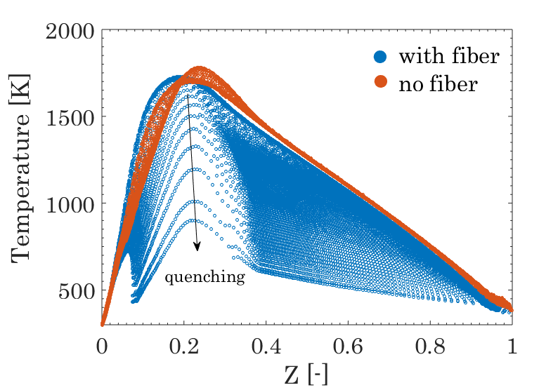
Another interesting effect of the fiber is the partial quenching of the flame (Figure 3) close to the fiber surface, due to its thermal inertia. In Figure 5c a scatterplot of the temperature with respect to the passive scalar (Equation 29) is reported, using all the points in the gas-phase region (). These scatterplots are typically used for turbulent flames, but in this case they are useful to describe in a compact way the temperature profiles orthogonal to the flame (). The scatterplot clearly shows a wide quenching zone (blue region) when the fiber is accounted for: focusing on the , the flame temperature, defined as the maximum temperature in the domain, decreases of K approaching the fiber along the flame front providing an incomplete combustion in this region. This effect is of primary importance since it leads to an accumulation of radicals and partial oxidation products at the fiber surface.
5.4 The effect of the oxygen concentration
In Figure 6a the numerical diameter decays of Cases 1, 2, 3 are presented and compared with the experiments. The numerical results have been shifted, so that time represents the ignition time. As expected, the diameter decay is very sensitive to the atmosphere composition: increasing the oxygen concentration leads to a higher temperature of (i) the flame and thus (ii) of the fiber. Both induce a more intense vaporization of the liquid, diminishing the droplet lifetime. The maximum temperature profile over time is reported in Figure 6d: after the ignition the flame temperature stabilizes at a constant value, which is higher for higher oxygen concentrations in the gas-phase. This can also be observed from the radial temperature profiles, taken along an horizontal line passing through the droplet center (for Cases 1, 3 in Figures 6b, 6c). The model predicts the experimental data with a reasonable accuracy, considering the error associated with the measurements (up to , as reported in yadav2017interferometric). Experimental errors can also be seen in the slight asymmetry of the temperature profiles. The difference in the maximum flame temperatures is K, with the peak for Case 3 slightly closer to the droplet surface. As reported in the last section of this paper, the agreement with the experimental results concerning the radial temperature profile improves including water condensation on the droplet surface.
Finally, it is worth analyzing the flame position with respect to the droplet interface (standoff ratio) for the three cases (Figure 6e). The flame diameter is indicated in Figure 3c and corresponds to the maximum horizontal distance of the isoline from the symmetry axis. The flame position with respect to the droplet surface slightly increases over time for all the three cases. The flame approaches the droplet surface increasing the oxygen concentration, since the stoichiometric condition at is satisfied closer to the droplet. The vicinity of the flame increases the vaporization rate from the droplet, further enhancing the effect of the higher oxygen concentration. This is in agreement to what observed by other authors farouk2011microgravity, farouk2012extinction.
5.5 The effect of gravity
The presence of a gravity field creates an upward buoyant flow ( m/s) once the flame is ignited and stabilized, which significantly influences the droplet combustion physics. The external convection forms a thin boundary layer, which considerably affects the heat and mass transport rates. To better discuss and highlight the effects of gravity, we simulated the cases in Table 3 at zero-gravity, imposing . The results are compared with the cases simulated in normal gravity in terms of flame temperature, standoff ratio (), flame geometry and internal motion. The presence of external convection influences:

- 1.
The droplet shape: under a convective field the droplet geometry is no longer spherical, due to the deformation induced by the flow. On principle this can affect the vaporization rate, since the surface area available for the vaporization is different. However, we noticed that for small droplets this is usually a minor effect saufi2019dropletsmoke++ and that the sphericity coefficient is 1 for most of the cases of our interest;
- 2.
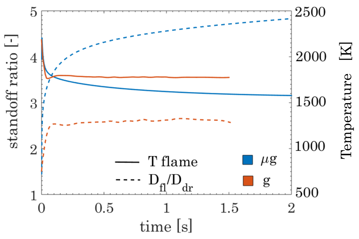
The flame geometry: in microgravity the flame is spherical and its distance from the droplet increases after the ignition, reaching a value of 4-5 times the droplet diameter (Figure 7a). As a consequence the flame temperature decreases, providing a possible radiative extinction if the flame diameter is large enough cuoci2017flame. On the other hand, in normal gravity the flame is axisymmetric and much closer to the droplet, maintaining its relative position almost constant in time (it is actually slightly increasing). This is due to the convective transfer of oxygen to the reactive region (much faster than pure diffusion), which satisfies the stoichiometric requirement of the flame front at a shorter distance. The average flame thickness is significantly reduced, especially in the lower part of the flame. As a result, the flame temperature is practically constant in time and higher than the case in microgravity (of 250 K). Moreover, the flame further approaches the droplet surface when the oxygen concentration increases. We found this effect to be similar both in microgravity and normal gravity, indicating that the presence of convection does not significantly affect the response of the flame distance to the oxygen concentration;
- 3.
The internal circulation: in microgravity the heat transfer in the liquid phase is mainly governed by conduction due to the absence of internal motion (if we neglect Marangoni flows). When gravity is present, the buoyancy-driven convection induces an internal motion in the liquid phase (shear stress continuity) which significantly enhances the internal heat transfer law1982recent. Figure 7b shows the two-phase velocity field for the burning droplet, highlighting the internal motion. The internal flow structure is commonly found in suspended droplets and resembles a Hill’s vortex sirignano1999fluid, having a toroidal core region within the droplet. The maximum velocity in the liquid phase ( cm/s) is an order of magnitude lower than the relative gas-phase velocity ( cm/s), in agreement to what observed by Prakash and Sirignano prakash1978liquid.
It is worth noticing that the gas-phase velocity field exhibits a substantial radial flow at the interface, due to the Stefan flow induced by the vaporization. Several authors observed that this radial flow leads to a significant reduction of the drag coefficient on the droplet jayawickrama2019effect, due to the expansion of the gas-phase boundary layer which significantly reduces the viscous force on the droplet. As an additional effect, this can make the liquid velocity field much less sensitive to the external convection, reducing the intensity of the internal motion. Following a fairly complex theoretical analysis, Sadhal sadhal1983flow observes that in the limit of extremely high radial flows the internal toroidal structure can be totally destroyed, due to the absence of a tangential component of the relative gas-phase velocity at the interface.
5.6 Distribution of the species in the gas phase

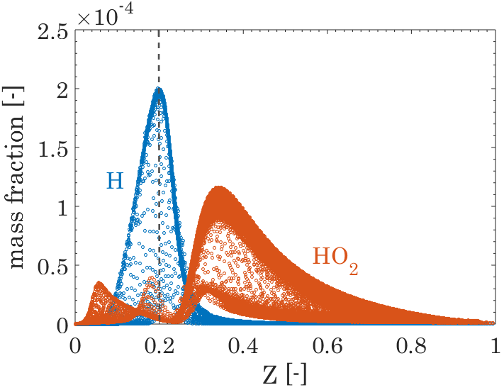
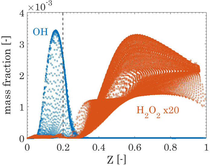

Once a passive scalar is defined (Equation 29), we can analyze the main species distribution (for Case 2 at s) along the flame coordinate. The results are reported in Figures 8 and 9, highlighting the . Analyzing the rate of production of the species, it is possible to get an insight on the methanol reactivity. As already reported, most of the species have a peak in the high scalar dissipation rate () region (low thickness), the lower part of the flame (Figure 8). The OH radical is slightly below the due to the need of O2 for its formation, while the H radical peak is at . The HO2 radical shows an interesting profile, with three peaks along : on the rich side, HO2 is mainly produced by O2+CH2OH HO2+CH2O, while on the lean side H+O2+(M)HO2+(M) is dominant, due to the high diffusivity of H, which escapes the flame front. The intermediate HO2 peak is due to the flame quenching at the fiber surface (clearly visible in the HO2 mass fraction map in Figure 8c), which decreases the temperature and stabilizes HO2. The important presence of HO2 for is also responsible for the hydrogen peroxide H2O2 formation (Figure 9b) through the abstraction reaction HO2+CH3OHH2O2+CH2OH, extensively investigated by other authors li2007comprehensive. At , OH recombination reaction (2OHH2O2) is the main responsible for H2O2 formation in the lean region. At there is an intermediate peak (not clearly visibile due to the very low concentration), still due to the flame quenching at the fiber which locally cools the flame.
The main combustion products are H2O and CO2 (Figure 9c), while CO is almost completely oxidized by OH at the flame front. With respect to the case without fiber, we notice a lower concentration of these species. It is worth noticing that CO, CO2 and H2O are present in significant amount at the droplet interface (), because of back diffusion from the flame. Differently from CO and CO2, water can condense on the droplet surface due to the low interface temperature ( 320 K). This will be analyzed in the next section.
5.7 Condensation of water
The water present among the combustion products in the gas-phase is miscible with methanol and it can condense on the droplet surface. If the liquid temperature is sufficiently high, water starts vaporizing as well and a two-component thermodynamics is established. This has been widely investigated in recent numerical and experimental works regarding alcohol combustion lee1992experimental, farouk2012extinction. From the modeling point of view it is only necessary to include the liquid species equation (Equation 7) and the correct evaporation rate for multicomponent mixtures (Table 1). As already reported, the boiling temperature is needed to trigger the boiling sub-model: in a two-component mixture (water and methanol) is not fixed with pressure, but it also depends on the local composition and it has to be calculated in every point in the liquid phase at every time step.
In order to highlight the effect of the absorbed water on the droplet combustion, we simulated the three cases in Table 3 including the water condensation flux. The results are reported in Figure 10. Referring to Figure 10a, we can identify two main vaporization regimes of the methanol-water mixture. During the first period the droplet is consumed faster when water absorption is accounted for: this happens because of the condensation heat released on the surface, which increases the temperature (4-5 K). Since methanol is (initially) the main component of the two-phase mixture, it vaporizes faster lee1992experimental. This can be clearly seen in Figure 10b, where the surface temperatures for the two cases are reported. Later on, the amount of condensed water becomes significant and the droplet global vaporization rate is retarded (also because of methanol dilution). This effect seems to be more enhanced at high temperatures (Case 3) due to the higher water concentration in the gas-phase. Moreover, the water absorbed at the surface is transported (by diffusion and internal convection) inside the liquid phase, close to the fiber. The vaporization enthalpy of the methanol-water mixture locally increases () and the internal boiling flux is diminished (Equation 25), further slowing the vaporization rate. At the droplet center the boiling conditions are reached for both cases (): while is constant for pure methanol vaporization, it constantly increases for the mixture because of water absorption () which changes the liquid composition (Figure 10c).
It is also worth analyzing the difference in the flame position with respect to the droplet surface (Figure 10d). The standoff ratio is higher due to the more intense methanol vaporization, which pushes the flame farther. This is reflected by the comparison of the radial temperature profiles (previously shown in Figure 6b, c) in Figures 11a, b: when water absorption is included, the temperature maximum slightly shifts away from the droplet and improves the agreement with the experimental data. Lee and Law lee1992experimental also report the existence of a final evaporation stage in which the condensed water starts to vaporize again once reached a significant concentration in the liquid. However, we did not notice this phenomena in our case probably because of the relatively low amount of water absorbed. In particular, we predict less than 10 (in mass) of water accumulation in the liquid phase at the end of the simulation (for all the cases). We found this effect to be negligible on the diameter decay (Figure 10a), since the vaporization rate is controlled by the internal boiling (mainly methanol) induced by the fiber.
To conclude, we want to mention the possibility to observe Marangoni effects in this configuration, i.e. internal flows caused by the gradients of surface tension along the interface hicks2010methanol. However, differently from microgravity systems, where this effect can significantly impact the combustion properties, in our cases the liquid motion is due to the external gas-phase convection and to the consequent shear-stress at the interface. Therefore, it is reasonable to assume the Marangoni flow to have a reduced impact on our simulation, since it is typically dominant in zero or very low Reynolds numbers () configurations raghavan2006surface. It is clear, however, that further investigations are needed: in particular towards the possibility of introducing advanced surface tension sub-models in multiphase CFD codes for droplet combustion in order to shed light on important effects such as Marangoni flows, contact angle effects and wetting phenomena.
6 Conclusions
In this paper we presented an interface-resolved numerical simulation of a methanol droplet suspended on a fiber in normal gravity, using a recent experimental work as a reference case. The multiphase VOF-based solver DropletSMOKE++ is adopted for the numerical modeling, because of its capability in describing in detail several physical phenomena such as the interface advection, the two-phase velocity field, the phase-change, the non-ideality of multicomponent mixtures, the combustion chemistry and the thermal interaction with the fiber. The high level of detail of the simulation allows to investigate interesting physical aspects related to suspended droplet combustion, in particular:
- 1.
The thermal perturbation of the fiber strongly affects the vaporization rate, conducting heat inside the liquid phase. The droplet interior is subjected to boiling, while the external surface evaporates by diffusion. A partial quenching of the flame occurs close to its surface, accumulating oxidized species;
- 2.
Higher oxygen concentrations increase the flame temperature, bring the flame closer to the droplet surface and diminish the droplet lifetime;
- 3.
The presence of a buoyant flow provides an axisymmetric flame geometry, with a lower standoff ratio and a higher flame temperature if compared to microgravity. Furthermore, the shear stress at the interface induces an internal circulation in the liquid phase, which enhances the internal heat transfer;
- 4.
The flame is thinner in the lower part of the droplet (high ), where we found the peak of most of the radical species. A brief analysis of the distribution of species in the gas phase shed light on the chemical behavior of H and HO2 radicals and on the quenching effect at the fiber;
- 5.
The water produced in the gas-phase condenses on the droplet surface, with two main effects: (i) an initial increase of the vaporization rate, due to the release of the condensation enthalpy at the droplet surface and (ii) a subsequent delay, because of water accumulation. The effect on the diameter decay is negligible, while the comparison of the radial temperature profiles slightly improves.
To conclude, we want to stress the importance of such fundamental analyses on isolated droplets to: (i) provide a general numerical support for the intense experimental activity on single droplet vaporization/combustion, including possible ways of improvement in the design of these systems (e.g. minimize the effect of the fiber) and (ii) the relevance for reduced numerical descriptions of sprays (e.g. LES), in particular for the development of accurate and reliable sub-models for mass transfer rates, drag force, Stefan flow, internal circulation etc. to be used in such complex numerical simulations.
In addition, we want to underline the generality and flexibility of this approach, which allows to easily introduce more complex kinetic mechanisms to investigate additional phenomena such as low temperature chemistry, soot formation and preferential vaporization, as well as the possibility to investigate multiple and interacting droplets.
Acknowledgments
We acknowledge the CINECA award under the ISCRA initiative, for the availability of high performance computing resources and support (ISCRA-B: HP10BGXWCZ).
| Variable | Refinement levels | O | |||
|---|---|---|---|---|---|
| n=1 | n=2 | n=3 | |||
| Tflame | 1711.29 | 1760.2 | 1759.95 | 1759.83 | 2.2 |
| Tsurface | 316.36 | 319.21 | 319.24 | 319.25 | 2.3 |
| COmax | 0.109 | 0.118 | 0.117 | 0.1165 | 1.8 |
| CO2,max | 0.248 | 0.236 | 0.234 | 0.233 | 1.8 |
| H2Omax | 0.171 | 0.146 | 0.143 | 0.142 | 2.3 |
| OHmax | 0.00311 | 0.00373 | 0.00364 | 0.0036 | 1.7 |
Appendix 0.A Grid refinement analysis
The sensitivity of the numerical results with respect to the mesh size is investigated. Case 2 (Table 3) is simulated at three levels of refinement: n=1 (37,000 cells), n=2 (92,000 cells) and n=3 (160,000 cells). The mesh is refined only in the fluid region, maintaining the proportions between the fine region (around the droplet) and the coarser one (outside the droplet). The analysis is reported in Table 4 at time s. The values are compared with the continuum value at zero grid spacing, evaluated adopting the Richardson extrapolation roache1993completed. The code shows convergence orders between 1.7 and 2.3 for the examined variables. Even though n=3 is the most accurate case, the refinement level n=2 (92,000 cells) has been used in this work, since the computational time is significantly reduced. Adopting this resolution, the average error for the reported variables remains between and .
References
- [1] G. Tryggvason, R. Scardovelli, S. Zaleski, Direct numerical simulations of gas–liquid multiphase flows, Cambridge University Press, 2011.
- [2] G. Faeth, Current status of droplet and liquid combustion, in: Energy and Combustion Science, Elsevier, 1979, pp. 149–182.
- [3] C. K. Law, Recent advances in droplet vaporization and combustion, Progress in energy and combustion science 8 (3) (1982) 171–201.
- [4] B. Helenbrook, C. Edwards, Quasi-steady deformation and drag of uncontaminated liquid drops, International journal of multiphase flow 28 (10) (2002) 1631–1657.
- [5] S. Okajima, S. Kumagai, Further investigations of combustion of free droplets in a freely falling chamber including moving droplets, in: Proceedings of the Combustion Institute, Vol. 15, Elsevier, 1975, pp. 401–407.
- [6] D. L. Dietrich, J. B. Haggard Jr, F. L. Dryer, V. Nayagam, B. D. Shaw, F. A. Williams, Droplet combustion experiments in spacelab, in: Proceedings of the Combustion Institute, Vol. 26, Elsevier, 1996, pp. 1201–1207.
- [7] A. Cuoci, M. Mehl, G. Buzzi-Ferraris, T. Faravelli, D. Manca, E. Ranzi, Autoignition and burning rates of fuel droplets under microgravity, Combustion and Flame 143 (3) (2005) 211–226.
- [8] T. I. Farouk, F. L. Dryer, Isolated n-heptane droplet combustion in microgravity: cool flames–two-stage combustion, Combustion and Flame 161 (2) (2014) 565–581.
- [9] A. Cuoci, A. E. Saufi, A. Frassoldati, D. L. Dietrich, F. A. Williams, T. Faravelli, Flame extinction and low-temperature combustion of isolated fuel droplets of n-alkanes, Proceedings of the Combustion Institute 36 (2) (2017) 2531–2539.
- [10] C. Morin, C. Chauveau, P. Dagaut, I. Goekalp, M. Cathonnet, Vaporization and oxidation of liquid fuel droplets at high temperature and high pressure: application to n-alkanes and vegetable oil methyl esters, Combustion science and technology 176 (4) (2004) 499–529.
- [11] M. Birouk, C. Chauveau, I. Gökalp, Turbulence effects on the combustion of single hydrocarbon droplets, Proceedings of the Combustion Institute 28 (1) (2000) 1015–1021.
- [12] C. Chauveau, M. Birouk, F. Halter, I. Gökalp, An analysis of the droplet support fiber effect on the evaporation process, International Journal of Heat and Mass Transfer 128 (2019) 885–891.
- [13] C. Avedisian, J. Yang, C. Wang, On low-gravity droplet combustion, Proceedings of the Royal Society of London. A. Mathematical and Physical Sciences 420 (1858) (1988) 183–200.
- [14] J. Yang, G. Jackson, C. Avedisian, Combustion of unsupported methanol/dodecanol mixture droplets at low gravity, in: Symposium (International) on Combustion, Vol. 23, Elsevier, 1991, pp. 1619–1625.
- [15] G. Jackson, C. Avedisian, J. Yang, Soot formation during combustion of unsupported methanol/toluene mixture droplets in microgravity, Proceedings of the Royal Society of London. Series A: Mathematical and Physical Sciences 435 (1894) (1991) 359–369.
- [16] Y. C. Liu, Y. Xu, M. C. Hicks, C. T. Avedisian, Comprehensive study of initial diameter effects and other observations on convection-free droplet combustion in the standard atmosphere for n-heptane, n-octane, and n-decane, Combustion and Flame 171 (2016) 27–41.
- [17] Y. Xu, M. C. Hicks, C. T. Avedisian, The combustion of iso-octane droplets with initial diameters from 0.5 to 5 mm: Effects on burning rate and flame extinction, Proceedings of the Combustion Institute 36 (2) (2017) 2541–2548.
- [18] M. A. Pfeil, L. J. Groven, R. P. Lucht, S. F. Son, Effects of ammonia borane on the combustion of an ethanol droplet at atmospheric pressure, Combustion and flame 160 (10) (2013) 2194–2203.
- [19] C. Chauveau, I. Gökalp, D. Segawa, T. Kadota, H. Enomoto, Effects of reduced gravity on methanol droplet combustion at high pressures, Proceedings of the Combustion Institute 28 (1) (2000) 1071–1077.
- [20] C. Chauveau, B. Vieille, I. Gökalp, D. Segawa, T. Kadota, A. Nakainkyo, Effects of gravitational acceleration on high pressure combustion of methanol droplets, Journal de Chimie Physique et de Physico-Chimie Biologique 96 (6) (1999) 1031–1037.
- [21] B. Shaw, J. Wei, Combustion of methanol droplets in air-diluent environments with reduced and normal gravity, Journal of Combustion 2012 (2012).
- [22] C. Chauveau, F. Halter, A. Lalonde, I. Gokalp, An experimental study on the droplet vaporization: effects of heat conduction through the support fiber, in: Proc. of 22 nd Annual Conference on Liquid Atomization and Spray Systems (ILASS Europe 2008), Vol. 59, 2008, p. 61.
- [23] O. A. George, J. Xiao, C. S. Rodrigo, R. Mercadé-Prieto, J. Sempere, X. D. Chen, Detailed numerical analysis of evaporation of a micrometer water droplet suspended on a glass filament, Chemical Engineering Science 165 (2017) 33–47.
- [24] Y. Wang, X. Chen, X. Wang, V. Yang, Vaporization of liquid droplet with large deformation and high mass transfer rate, ii: Variable-density, variable-property case, Journal of Computational Physics 394 (2019) 1–17.
- [25] B. Wang, A. Kronenburg, G. L. Tufano, O. T. Stein, Fully resolved DNS of droplet array combustion in turbulent convective flows and modelling for mixing fields in inter-droplet space, Combustion and Flame 189 (2018) 347–366.
- [26] Y. Jin, B. Shaw, Computational modeling of n-heptane droplet combustion in air–diluent environments under reduced-gravity, International Journal of Heat and Mass Transfer 53 (25-26) (2010) 5782–5791.
- [27] N. Ghata, B. D. Shaw, Computational modeling of unsupported and fiber-supported n-heptane droplet combustion in reduced gravity: a study of fiber effects, Combustion Science and Technology 187 (1-2) (2015) 83–102.
- [28] A. K. Yadav, A. Chowdhury, A. Srivastava, Interferometric investigation of methanol droplet combustion in varying oxygen environments under normal gravity, International Journal of Heat and Mass Transfer 111 (2017) 871–883.
- [29] A. Saufi, A. Frassoldati, T. Faravelli, A. Cuoci, DropletSMOKE++: A comprehensive multiphase CFD framework for the evaporation of multidimensional fuel droplets, International Journal of Heat and Mass Transfer 131 (2019) 836–853.
- [30] A. Saufi, R. Calabria, F. Chiariello, A. Frassoldati, A. Cuoci, T. Faravelli, P. Massoli, An experimental and CFD modeling study of suspended droplets evaporation in buoyancy driven convection, Chemical Engineering Journal (2019) 122006.
- [31] C. W. Hirt, B. D. Nichols, Volume of fluid (VOF) method for the dynamics of free boundaries, Journal of computational physics 39 (1) (1981) 201–225.
- [32] J. Roenby, H. Bredmose, H. Jasak, A computational method for sharp interface advection, Royal Society open science 3 (11) (2016) 160405.
- [33] C. J. Greenshields, OpenFOAM user guide, OpenFOAM Foundation Ltd, version 3 (1) (2015).
- [34] R. B. Bird, Transport phenomena, Applied Mechanics Reviews 55 (1) (2002) R1–R4.
- [35] J. M. Smith, Introduction to chemical engineering thermodynamics, ACS Publications, 1950.
- [36] J. Reutzsch, C. Kieffer-Roth, B. Weigand, A consistent method for direct numerical simulation of droplet evaporation, Journal of Computational Physics (2020) 109455.
- [37] J. Brackbill, D. B. Kothe, C. Zemach, A continuum method for modeling surface tension, Journal of computational physics 100 (2) (1992) 335–354.
- [38] S. Popinet, An accurate adaptive solver for surface-tension-driven interfacial flows, Journal of Computational Physics 228 (16) (2009) 5838–5866.
- [39] A. Q. Raeini, M. J. Blunt, B. Bijeljic, Modelling two-phase flow in porous media at the pore scale using the volume-of-fluid method, Journal of Computational Physics 231 (17) (2012) 5653–5668.
- [40] V. Vukčević, H. Jasak, I. Gatin, Implementation of the ghost fluid method for free surface flows in polyhedral finite volume framework, Computers & Fluids 153 (2017) 1–19.
- [41] S. Popinet, Numerical models of surface tension, Annual Review of Fluid Mechanics 50 (2018) 49–75.
- [42] J. Palmore Jr, O. Desjardins, A volume of fluid framework for interface-resolved simulations of vaporizing liquid-gas flows, Journal of Computational Physics 399 (2019) 108954.
- [43] J.-R. Yang, S.-C. Wong, On the discrepancies between theoretical and experimental results for microgravity droplet evaporation, International Journal of Heat and Mass Transfer 44 (23) (2001) 4433–4443.
- [44] Y. Liu, Y. Xu, C. Avedisian, M. Hicks, The effect of support fibers on micro-convection in droplet combustion experiments, Proceedings of the Combustion Institute 35 (2) (2015) 1709–1716.
- [45] C. T. Avedisian, G. S. Jackson, Soot patterns around suspended n-heptane droplet flames in a convection-free environment, Journal of Propulsion and Power 16 (6) (2000) 974–979.
- [46] A. Cuoci, A. Frassoldati, T. Faravelli, E. Ranzi, OpenSMOKE++: An object-oriented framework for the numerical modeling of reactive systems with detailed kinetic mechanisms, Computer Physics Communications 192 (2015) 237–264.
- [47] C. L. Yaws, The Yaws Handbook of Physical Properties for Hydrocarbons and Chemicals: Physical Properties for More Than 54,000 Organic and Inorganic Chemical Compounds, Coverage for C1 to C100 Organics and Ac to Zr Inorganics, Gulf Professional Publishing, 2015.
- [48] A. Fredenslund, R. L. Jones, J. M. Prausnitz, Group-contribution estimation of activity coefficients in nonideal liquid mixtures, AIChE Journal 21 (6) (1975) 1086–1099.
- [49] G. Strang, On the construction and comparison of difference schemes, SIAM journal on numerical analysis 5 (3) (1968) 506–517.
- [50] A. Cuoci, A. Frassoldati, T. Faravelli, E. Ranzi, A computational tool for the detailed kinetic modeling of laminar flames: Application to C2H4/CH4 coflow flames, Combustion and Flame 160 (5) (2013) 870–886.
- [51] P. S. Veloo, Y. L. Wang, F. N. Egolfopoulos, C. K. Westbrook, A comparative experimental and computational study of methanol, ethanol, and n-butanol flames, Combustion and Flame 157 (10) (2010) 1989–2004.
- [52] E. Ranzi, A. Frassoldati, A. Stagni, M. Pelucchi, A. Cuoci, T. Faravelli, Reduced kinetic schemes of complex reaction systems: fossil and biomass-derived transportation fuels, International Journal of Chemical Kinetics 46 (9) (2014) 512–542.
- [53] E. Ranzi, A. Sogaro, P. Gaffuri, G. Pennati, T. Faravelli, A wide range modeling study of methane oxidation, Combustion science and technology 96 (4-6) (1994) 279–325.
- [54] W. K. Metcalfe, S. M. Burke, S. S. Ahmed, H. J. Curran, A hierarchical and comparative kinetic modeling study of C1- C2 hydrocarbon and oxygenated fuels, International Journal of Chemical Kinetics 45 (10) (2013) 638–675.
- [55] S. M. Burke, U. Burke, R. Mc Donagh, O. Mathieu, I. Osorio, C. Keesee, A. Morones, E. L. Petersen, W. Wang, T. A. DeVerter, et al., An experimental and modeling study of propene oxidation. part 2: Ignition delay time and flame speed measurements, Combustion and Flame 162 (2) (2015) 296–314.
- [56] A. Burcat, B. Ruscic, et al., Third millenium ideal gas and condensed phase thermochemical database for combustion (with update from active thermochemical tables)., Tech. rep., Argonne National Lab.(ANL), Argonne, IL (United States) (2005).
- [57] A. Stagni, A. Frassoldati, A. Cuoci, T. Faravelli, E. Ranzi, Skeletal mechanism reduction through species-targeted sensitivity analysis, Combustion and Flame 163 (2016) 382–393.
- [58] P. Pepiot-Desjardins, H. Pitsch, An efficient error-propagation-based reduction method for large chemical kinetic mechanisms, Combustion and Flame 154 (1-2) (2008) 67–81.
- [59] T. Poinsot, D. Veynante, Theoretical and numerical combustion, RT Edwards, Inc., 2005.
- [60] R. Bilger, S. Stårner, R. Kee, On reduced mechanisms for methane air combustion in nonpremixed flames, Combustion and Flame 80 (2) (1990) 135–149.
- [61] T. Farouk, F. Dryer, Microgravity droplet combustion: effect of tethering fiber on burning rate and flame structure, Combustion Theory and Modelling 15 (4) (2011) 487–515.
- [62] T. I. Farouk, F. L. Dryer, On the extinction characteristics of alcohol droplet combustion under microgravity conditions–a numerical study, Combustion and flame 159 (10) (2012) 3208–3223.
- [63] W. A. Sirignano, Fluid dynamics and transport of droplets and sprays, Cambridge university press, 1999.
- [64] S. Prakash, W. Sirignano, Liquid fuel droplet heating with internal circulation, International Journal of Heat and Mass Transfer 21 (7) (1978) 885–895.
- [65] T. R. Jayawickrama, N. E. L. Haugen, M. U. Babler, M. A. Chishty, K. Umeki, The effect of stefan flow on the drag coefficient of spherical particles in a gas flow, International Journal of Multiphase Flow 117 (2019) 130–137.
- [66] S. S. Sadhal, P. S. Ayyaswamy, Flow past a liquid drop with a large non-uniform radial velocity, Journal of Fluid Mechanics 133 (1983) 65–81.
- [67] J. Li, Z. Zhao, A. Kazakov, M. Chaos, F. L. Dryer, J. J. Scire Jr, A comprehensive kinetic mechanism for CO, CH2O, and CH3OH combustion, International Journal of Chemical Kinetics 39 (3) (2007) 109–136.
- [68] A. Lee, C. K. Law, An experimental investigation on the vaporization and combustion of methanol and ethanol droplets, Combustion science and technology 86 (1-6) (1992) 253–265.
- [69] M. C. Hicks, V. Nayagam, F. A. Williams, Methanol droplet extinction in carbon-dioxide-enriched environments in microgravity, Combustion and flame 157 (8) (2010) 1439–1445.
- [70] V. Raghavan, D. N. Pope, D. Howard, G. Gogos, Surface tension effects during low-reynolds-number methanol droplet combustion, Combustion and Flame 145 (4) (2006) 791–807.
- [71] P. J. Roache, P. M. Knupp, Completed richardson extrapolation, Communications in Numerical Methods in Engineering 9 (5) (1993) 365–374.