Description of the newly observed $\Xi_{c}^{0}$ states as molecular states

During the past several decades, many narrow baryons with a heavy charm quark, a light up or down quark, and a strange quark have been reported by the LHCb,CDF Collaboration and so on Tanabashi:2018oca. Very recently, three other neutral resonances $\Xi_{c}^{*0}$ named $\Xi_{c}(2923)^{0}$, $\Xi_{c}(2939)^{0}$, and $\Xi_{c}(2965)^{0}$ have been observed in the $K^{-}\Lambda_{c}^{+}$ mass spectra by the LHCb Collaboration Aaij:2020yyt. The observed resonance masses and widths are

respectively. From the observed decay mode, the isospin of these three states are $1/2$. Although the quantum numbers of these states remain undetermined, it is very helpful to understand the spectroscopy of the heavy baryons containing $c$ and $s$ quark.

Due to their observed decay mode, the new structures $\Xi_{c}(2923)^{0}$, $\Xi(2938)^{0}$, and $\Xi(2964)^{0}$ contain at least three different valence quark components. In other word, these states may be candidates of conventional three-quark state. Indeed, the QCD sum rule suggests that the newly observed states $\Xi_{c}(2923)^{0}$, $\Xi(2938)^{0}$, and $\Xi(2964)^{0}$ are most likely to be considered as the $P$-wave $\Xi_{c}^{{}^{\prime}}$ baryons with the spin-parity $J^{p}=1/2^{-}$ or $J^{p}=3/2^{-}$ Yang:2020zjl. In Ref. Wang:2020gkn the $\Xi_{c}(2923)^{0}$, $\Xi(2938)^{0}$, and $\Xi(2964)^{0}$ ware suggested to be $1P$ $\Xi_{c}^{{}^{\prime}}$ state with spin-parity $J^{P}=3/2^{-}$ or $J^{P}=5/2^{-}$ in the chiral quark model. In Ref. Lu:2020ivo the two-body strong decays of the $\Xi_{c}(2923)^{0}$, $\Xi(2938)^{0}$, and $\Xi(2964)^{0}$ were calculated by employing the ${}^{3}P_{0}$ approach with the conclusion that the $\Xi_{c}(2923)^{0}$ and $\Xi(2938)^{0}$ can be $1P$ $\Xi_{c}^{{}^{\prime}}$ states, and the $\Xi(2964)^{0}$ can be regarded as the $2S$ $\Xi_{c}^{{}^{\prime}}$ state. The lattice QCD calculation was also performed and try to determine their quantum numbers Bahtiyar:2020uuj.

Although the authors in Refs. Yang:2020zjl; Wang:2020gkn; Lu:2020ivo; Bahtiyar:2020uuj try to assign these states into the conventional three-quark frames, it is obvious that the inner structure of $\Xi_{c}(2923)^{0}$, $\Xi(2938)^{0}$, and $\Xi(2964)^{0}$ are not finally determined. And another interpretation is treating them as $D\Lambda-D\Sigma$ molecular states, because the smallest mass gaps between the newly observed $\Xi_{c}$ baryons and the ground $\Xi_{c}$, about 450 MeV, is large enough to excite a light quark-antiquark pair to form a hadronic molecular. Indeed, it is shown in Refs. JimenezTejero:2009vq; Yu:2018yxl; Nieves:2019jhp that the interaction between $D$ meson and $\Lambda$ or $\Sigma$ baryon is strong enough to form a bound state with a mass about 2930 MeV.

The key point in this work is to explain whether the $\Xi_{c}(2923)^{0}$, $\Xi(2938)^{0}$, and $\Xi(2964)^{0}$ can be considered as a molecular state. Here, we will consider the strong $\Xi_{c}^{*}\to\Lambda_{c}^{+}K^{-}$,$\Sigma_{c}^{+}K^{-}$, and $\Xi_{c}^{+}\pi^{-}$ decays of the $\Xi_{c}(2923)^{0}$,
$\Xi(2938)^{0}$, and $\Xi(2964)^{0}$ with the possible quantum numbers $J^{p}=1/2^{\pm}$ and $3/2^{\pm}$ using an effective Lagrangian approach. The approach is based on the hypothesis that the $\Xi_{c}^{*}$ is a hadronic molecule state of $D\Lambda$-$D\Sigma$. The coupling of the $\Xi_{c}^{*}$ to the constituents is described by the effective Lagrangian. The corresponding coupling constant $g_{\Xi_{c}^{*}\Lambda{}D}$ and $g_{\Xi_{c}^{*}\Sigma{}D}$ are determined by the compositeness condition $Z=0$ Faessler:2007gv; Faessler:2007us; Dong:2009tg; Dong:2010xv; Dong:2010gu, which implies that the renormalization constant of the hadron wave function is set equal to zero. By constructing a phenomenological Lagrangian including the couplings of the bound state to its constituents and the constituents with other particles we calculated one-loop diagrams describing different decays of the molecular states.

This work is organized as follows. The theoretical formalism is explained in Sec. 2. The predicted partial decay widths are presented in Sec. 3, followed by a short summary in the last section.

In the molecular scenario, the details of the calculations for $\Xi_{c}^{0}\to\Lambda_{c}^{+}K^{-}$, $\Xi_{c}^{0}\to\Sigma_{c}^{+}K^{-}$, and $\Xi_{c}^{0}\to\Xi_{c}^{+}\pi^{-}$ are presented for $\Xi_{c}$ state with two different total angular momentum $J$ possibilities. The molecular structure of the $\Xi_{c}^{*}$ baryon with quantum numbers $J^{p}=1/2^{\pm}$ is described by the Lagrangian Dong:2010gu

while for the choice $J^{p}=3/2^{\pm}$ the Lagrangian contains a derivative

where $\Gamma$ is the corresponding Dirac matrix related to the spin-parity of the $\Xi_{c}^{*}$. In particular, for $J^{p}=1/2^{+},3/2^{-}$ we have $\Gamma=\gamma^{5}$ while for $J^{p}=1/2^{-},3/2^{+}$ the Dirac structure $\Gamma=1$. In the Lagrangian, an effective correlation function $\Phi(y^{2})$ is introduced to reflect the distribution of two constituents in the hadronic molecular $\Xi_{c}^{*}$ state. The introduced correlation function also makes the Feynman diagrams finite in the ultraviolet region of Euclidean space, which indicates that the Fourier transformation of the correlation function should drop fast enough in the ultraviolet region. Here we choose the Fourier transformation of the correlation in the Gaussian form Faessler:2007gv; Faessler:2007us; Dong:2009tg; Dong:2010xv; Dong:2010gu,

with $\alpha$ being the size parameter which characterize the distribution of components inside the molecule. Though the value of $\alpha$ could not be determined from first principles, it is usually chosen to be about $1$ GeV in the literature Faessler:2007gv; Faessler:2007us; Dong:2009tg; Dong:2010xv; Dong:2010gu. In this work, we set $\Lambda=1.0$ GeV.

With the help of the effective Lagrangian in Eq.( 1) and Eq.( 2), we can obtain the self energy of the $\Xi_{c}^{*}$

where $k_{0}^{2}=m^{2}_{\Xi_{c}^{*}}$ with $k_{0},m^{*}_{\Xi_{c}}$ denoting the four momenta and mass of the $\Xi_{c}^{*}$, respectively, $k_{1}$, $m_{D}$, and $m_{\Lambda}$, $m_{\Sigma}$ are the four-momenta, the mass of the $D$ meson, and the mass of the $\Lambda$ baryon, the mass of the $\Sigma$ baryon, respectively. The coupling constant $g_{\Xi_{c}^{*}\Lambda\bar{D}}$ and $g_{\Xi_{c}^{*}\Sigma{}D}$ is determined by the compositeness condition Weinberg:1962hj; Salam:1962ap. It implies that the renormalization constant of the hadron wave function is set equal to zero with

where the $x_{AB}$ is the probability to find the $\Xi_{c}^{*}$ in the hadronic state $AB$ with the normalization $x_{D\Lambda}+x_{D\Sigma}=1.0$. And the $\Sigma^{3/2-T}_{\Xi_{c}^{*}}$ is the transverse part of the self-energy operator $\Sigma^{3/2}_{\Xi_{c}^{*}}$, related to $\Sigma^{3/2}_{\Xi_{c}^{*}}$ via

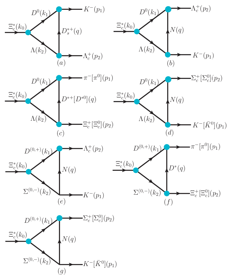
Fig. (2) shows the hadronic decay of the $\Lambda{}D-\Sigma{D}$ molecular state into the $\Lambda_{c}^{+}K^{-}$,$\Xi_{c}^{+}\pi^{-}$, and $\Sigma_{c}^{+}K^{-}$ final states occuring by exchanging nucleon, $D_{s}^{*}$ meson, and $D^{*}$ meson. To compute the amplitudes of the diagrams shown in Fig.( 2), we need the effective Lagrangian densities for the relevant interaction vertices. In Refs. Hofmann:2005sw; Montana:2017kjw, coupling of the vector meson to charm baryons are described from effective Lagrangians, which are obtained using the hidden gauge formalism and assuming SU(4) symmetry:

where the coupling constant $g=6.6$ is from Ref. Hofmann:2005sw. The symbol $V_{\mu}$ represents the vector fields of the 16-plet of the $\rho$, given by

and $B$ is the tensor of baryons belonging to the 20-plet of $p$

where the indices $i,j,k$ of $B^{ijk}$ denote the quark content of the baryon fields with the identification $1\leftrightarrow{u},2\leftrightarrow{d},3\leftrightarrow{}s$,and $4\leftrightarrow{}c$.

To evaluate the diagrams in Fig.( 2), in addition to the Lagrangian in Eq.( 1), Eq.( 2), and Eq.( 8), the following effective Lagrangians, responsible for vector mesons and pseudoscalar mesons interactions are needed as well Hofmann:2005sw

where $P$ is the $SU(4)$ pseudoscalar meson matrices, and $\langle...\rangle$ in the trace over the $SU(4)$ matrices. The meson matrices are Hofmann:2005sw

The coupling $g_{h}$ is fixed from the strong decay width of $K^{*}\to{}K\pi$. With the help of Eq. (12), the two-body decay width $\Gamma(K^{*+}\to{}K^{0}\pi^{+})$ is related to $g_{h}$ as

where ${\cal{P}}_{\pi{}K^{*}}$ is the three-momentum of the $\pi$ in the rest frame of the $K^{*}$. Using the experimental strong decay width($\Gamma_{K^{*+}}=50.3\pm 0.8$ MeV) and the masses of the particles needed in the present work are listed in Table. (1) we obtain $g=4.64$ Tanabashi:2018oca.

The vertexes for the meson-baryon interaction are needed and the form in the $SU(3)$ sector is given by the chiral Lagrangian Garzon:2012np

where $F=0.51$,$D=0.75$ Garzon:2012np and at lowest order in the pseudoscalar field $u^{\mu}=-\sqrt{2}\partial^{\mu}\phi/f$, with $f=93$ MeV. And ${\cal{B}}$ and $\phi$ is now the $SU(3)$ matrix of the baryon octet and meson, respectively.

Moreover, the effective Lagrangians for the $DN\Lambda_{c}$ and $DN\Sigma_{c}$ couplings are Xie:2015zga; Huang:2016ygf

with $\vec{\tau}$ being the usual Pauli matrices. The coupling constant $g_{\Lambda_{c}pD}=10.7^{+5.3}_{-4.3}$ and $g_{\Sigma_{c}pD}=-2.69$ are borrowed from Refs. Xie:2015zga; Huang:2016ygf; Khodjamirian:2011sp, where we take the central values $g_{\Lambda_{c}pD}=10.7$ in our calculation.

With the above vertices, the amplitudes of the triangle diagrams of Fig.( 2), evaluated in the center of mass frame of final states, are

References

• (1) M. Tanabashi et al. [Particle Data Group], Review of Particle Physics, Phys. Rev. D 98, 030001 (2018).
• (2) R. Aaij et al. [LHCb], Observation of new Ξc0\Xi_{c}^{0} baryons decaying to Λc+​K−\Lambda_{c}^{+}K^{-}, [arXiv:2003.13649 [hep-ex]].
• (3) H. Yang, H. Chen and Q. Mao, Identifying the Ξc0\Xi_{c}^{0} baryons observed by LHCb as PP-wave Ξc′\Xi_{c}^{\prime} baryons, [arXiv:2004.00531 [hep-ph]].
• (4) K. Wang, L. Xiao and X. Zhong, Understanding the newly observed Ξc0\Xi_{c}^{0} states through their decays, [arXiv:2004.03221 [hep-ph]].
• (5) Qi-Fang. Lü, Canonical interpretations of the newly observed Ξc​(2923)0\Xi_{c}(2923)^{0}, Ξc​(2939)0\Xi_{c}(2939)^{0} and Ξc​(2965)0\Xi_{c}(2965)^{0} resonances, [arXiv:2004.02374 [hep-ph]].
• (6) H. Bahtiyar, K. U. Can, G. Erkol, P. Gubler, M. Oka and T. T. Takahashi, Charmed baryon spectrum from lattice QCD near the physical point, [arXiv:2004.08999 [hep-lat]].
• (7) C. E. Jimenez-Tejero, A. Ramos and I. Vidana, Dynamically generated open charmed baryons beyond the zero range approximation, Phys. Rev. C 80, 055206 (2009).
• (8) Q. X. Yu, R. Pavao, V. R. Debastiani and E. Oset, Description of the Ξc\Xi_{c} and Ξb\Xi_{b} states as molecular states, Eur. Phys. J. C 79, 167 (2019).
• (9) J. Nieves, R. Pavao and L. Tolos, Ξc\Xi_{c} and Ξb\Xi_{b} excited states within a SU(6)lsf×{\rm SU(6)}_{\rm lsf}\times HQSS model, Eur. Phys. J. C 80, 22 (2020).
• (10) A. Faessler, T. Gutsche, V. E. Lyubovitskij and Y. L. Ma, Strong and radiative decays of the Ds​0∗​(2317)D_{s0}^{*}(2317) meson in the D​KDK-molecule picture, Phys. Rev. D 76, 014005 (2007).
• (11) A. Faessler, T. Gutsche, V. E. Lyubovitskij and Y. L. Ma, D∗​KD^{*}K molecular structure of the Ds​1​(2460)D_{s1}(2460) meson, Phys. Rev. D 76, 114008 (2007).
• (12) Y. Dong, A. Faessler, T. Gutsche and V. E. Lyubovitskij, Strong two-body decays of the Λc​(2940)+\Lambda_{c}(2940)^{+} in a hadronic molecule picture, Phys. Rev. D 81, 014006 (2010).
• (13) Y. Dong, A. Faessler, T. Gutsche, S. Kumano and V. E. Lyubovitskij, Radiative decay of Λc​(2940)+\Lambda_{c}(2940)^{+} in a hadronic molecule picture, Phys. Rev. D 82, 034035 (2010).
• (14) Y. Dong, A. Faessler, T. Gutsche and V. E. Lyubovitskij, Charmed baryon Sigmac(2800) as a ND hadronic molecule, Phys. Rev. D 81, 074011 (2010).
• (15) S. Weinberg, Elementary particle theory of composite particles, Phys. Rev. 130, 776 (1963).
• (16) A. Salam, Lagrangian theory of composite particles, Nuovo Cim. 25, 224 (1962).
• (17) J. Hofmann and M. F. M. Lutz, Coupled-channel study of crypto-exotic baryons with charm, Nucl. Phys. A 763, 90 (2005).
• (18) G. Montan~\tilde{n}a, A. Feijoo and à. Ramos, A meson-baryon molecular interpretation for some Ωc\Omega_{c} excited states, Eur. Phys. J. A 54, 64 (2018).
• (19) E. J. Garzon and E. Oset, Effects of pseudoscalar-baryon channels in the dynamically generated vector-baryon resonances, Eur. Phys. J. A 48, 5 (2012).
• (20) J. J. Xie, Y. B. Dong and X. Cao, Role of the Λc+​(2940)\Lambda^{+}_{c}(2940) in the π−​p→D−​D0​p\pi^{-}p\to D^{-}D^{0}p reaction close to threshold, Phys. Rev. D 92, 034029 (2015).
• (21) Y. Huang, J. He, J. J. Xie and L. S. Geng, Production of the Λc​(2940)\Lambda_{c}(2940) by kaon-induced reactions on a proton target, Phys. Rev. D 99, 014045 (2019).
• (22) A. Khodjamirian, C. Klein, T. Mannel and Y. M. Wang, How much charm can PANDA produce?, Eur. Phys. J. A 48, 31 (2012).
• (23) J. He, Understanding spin parity of Pc​(4450)P_{c}(4450) and Y⁡(4274)Y(4274) in a hadronic molecular state picture, Phys. Rev. D 95, 074004 (2017).