Model studies of fluctuations in the background for jets in heavy ion collisions
Abstract
Jets produced in high energy heavy ion collisions are quenched by the quark gluon plasma. Measurements of these jets are influenced by the methods used to suppress and subtract the large, fluctuating background and the assumptions inherent in these methods. We compare the measurements of the background in Pb+Pb collisions at = 2.76 TeV by the ALICE Collaboration (B. Abelev et al., J. High Energy Phys. , 053) to calculations in TennGen (a data-driven random background generator) and PYTHIA Angantyr. A detailed understanding of the width of these fluctuations is important for reducing uncertainties due to unfolding and extending measurements to lower momenta and larger resolution parameters. The standard deviation of the energy in random cones in TennGen is approximately in agreement with the form predicted in the ALICE paper, with deviations of 1–6%. The standard deviation of energy in random cones in Angantyr exceeds the same predictions by approximately 13%. Deviations in both models can be explained by the assumption that the single-particle is a gamma distribution in the derivation of the prediction, whereas the model uses a different distribution. This indicates that model comparisons are potentially sensitive to the treatment of the background. We demonstrate that unfolding methods used to remove background fluctuations from jets can affect the comparisons between models and data, . Our findings suggest the need to more carefully consider methods for comparing simulations and data.
pacs
25.75.-q,25.75.Gz,25.75.BhI Introduction
A hot, dense, strongly interacting liquid of quarks and gluons called the Quark Gluon Plasma (QGP) is briefly created in high energy heavy ion collisions Adcox:2004mh; Adams:2005dq; Back:2004je; Arsene:2004fa. Two of the key signatures of the formation of the QGP are hydrodynamical flow and jet quenching. The strong azimuthal asymmetry in the final state particles’ momenta is a signature of hydrodynamical flow. There are many measurements of jets which can, in principle, provide quantitative constraints on the properties of the medium Connors:2017ptx. While there have been some constraints on the properties of the medium from measurements of jets Burke:2013yra; JETSCAPE:2021ehl, the era of quantitative measurements is just beginning.
Improving quantitative constraints on the medium using jet measurements requires a quantitative understanding of the background. The correlations due to flow lead to an anisotropic background, which can in turn influence jet measurements. At the Relativistic Heavy Ion Collider (RHIC), mixed events were able to successfully describe the background in measurements of hadron-jet correlations Adamczyk:2017yhe, indicating that the background is dominated by random combinations of particles. Studies of the background at the Large Hadron Collider (LHC) by the ALICE Collaboration found that the distribution of background energy density measured by using random cones with the leading jet removed were described well by predictions for a random background with correlations due to flow ALICE:2012nbx.
We study the measurements in ALICE:2012nbx in two models. We compare to a data-driven random background generator, TennGen TennGenGITHUB, which uses the measured single-particle spectra and flow to generate a realistic background without any jets. We also use PYTHIA Angantyr Bierlich:2018xfw, a Monte Carlo generator based on PYTHIA 8.2Bierlich:2018xfw; Sjostrand:2006za, which models heavy ion collisions as a superposition of nucleon-nucleon collisions. We stress that an understanding of this background is important for reducing uncertainties in jet measurements, which would help extend measurements in heavy ion collisions to higher resolution parameters and lower momenta. The uncertainties due to unfolding are driven by the width of the distribution rather than the overall level of the background.
We emphasize that while models may simplify the physics of heavy ion collisions they still contain background and background fluctuations. We examine different approaches to unfolding to correct for background fluctuations in models. We discuss how the presence of this background can affect observables in Monte Carlo simulations, underscoring the need for a treatment of background in model studies similar to that in data.
II Simulations
II.1 TennGen
The measured single particle double differential spectra for , , and from Abelev:2012hxa are fit to a Boltzmann-Gibbs blast wave distribution Ristea:2013ara; Schnedermann:1993ws
| (1) |
where is the transverse momentum, is the rapidity, is the normalization, is the mass of the particle, is the surface velocity, is an exponent describing the evolution of the velocity profile, and is the kinetic freeze-out temperature. The and are modified Bessel functions. The reduced radius, , is integrated over from 0 to 1. The multiplicity of each particle species is determined from charged particle ratios Abelev:2013vea and is scaled up assuming a constant charged particle multiplicity per unit pseudorapidity, . This is a reasonable approximation for the pseudorapidity region used in this analysis, . The multiplicities are determined from measurements of the charged particle multiplicities in ALICE at the LHC Aamodt:1313050. Only the centrality bins in Abelev:2013vea are available (0–5%, 5–10%, 10–20%, 20–30%, 30–40%, and 40–50%) and there are no fluctuations in the multiplicity within a centrality bin. Only charged hadrons are generated for this analysis. Furthermore, all particles produced from TennGen are uncorrelated except through correlations with the event planes.
The azimuthal asymmetry in heavy ion collisions is decomposed using
| (2) |
where is the number of particles, the coefficients are defined as = , and is the azimuthal position of the track. The symmetry planes are set to zero for even for simplicity. This differs from the physical correlations between the second and fourth event plane, which have been observed to fluctuate relative to each other Aad:2014fla. While this difference between the TennGen simulation and measurements would affect observables sensitive to flow, the simulation is only intended to capture most of the correlations due to flow and not intended as an exact quantitative reproduction. The for odd are randomly thrown from a flat distribution for the odd , roughly matching correlations observed in data Aad:2014fla. A random is thrown from the distribution in Eq. 1, which is then used to determine the . This is used to construct an azimuthal distribution of particles at the momentum and a random is drawn from that distribution. This is repeated for all the particles in the event. The can also be set to zero to remove the impact of correlations due to flow, leaving a uniform distribution of particles.
When the are included, the -dependent from Adam:2016nfo are fit to a polynomial for . For , a rapidity-even comparable to and has been observed Luzum:2010fb; ATLAS:2012at; Retinskaya:2012ky, but it is difficult to measure and is still poorly constrained. To roughly match these measurements, we use , which will give a negative for low and a positive for high , roughly conserving momentum. The azimuthal coordinate is then randomly drawn from Eq. 2. The pseudorapidity () is randomly drawn from a uniform distribution for 0.9. For each centrality bin and combination of , 60000 events are generated. For the 0–10% centrality bin, the 0–5% and 5–10% bins are combined. The code for TennGen is available on Github TennGenGITHUB.
II.2 Angantyr
PYTHIA Angantyr Bierlich:2018xfw is a Monte Carlo model for heavy ion collisions included in PYTHIA 8 Bierlich:2018xfw; Sjostrand:2006za. It is primarily a superposition of nucleon-nucleon collisions and includes inelastic collisions, single-diffractive, double-diffractive, and absorptive collisions using a model with fluctuating radii. The fluctuating nucleon radii result in a fluctuating nucleon-nucleon cross section. This further results in multiplicity fluctuations. Angantyr includes hard scatterings, event-by-event multiplicity fluctuations, and multiparton interactions. Angantyr does not contain flow (string shoving is not enabled in this analysis) or jet quenching. As such, it is a good baseline for collisions in the absence of a QGP.
Default parameters are used and minimum bias Pb+Pb collisions at = 2.76 TeV and minimum bias Au+Au collisions at = 200 GeV were generated. The centrality is determined using the centrality class implemented in Rivet Buckley:2010ar, which uses the multiplicity in the forward pseudorapidity regions matching the ALICE V0-A (2.8 5.1) and V0-C (-3.7 -1.7) acceptance ALICE:2004ftm and bins the events in terms of the multiplicity in these regions in Angantyr.
II.3 Reconstruction efficiency
The measurements in ALICE:2012nbx did not include corrections for detector effects so we implement an approximate single track reconstruction efficiency, the dominant effect, to make these model calculations more realistic. We use a parametrized -dependent efficiency roughly matching the efficiency of the ALICE detector in Abelev:2014ffa when comparing to ALICE:2012nbx.
III Results
III.1 Background density
| 0.4 | |
| ghost max. rapidity | 2.0 |
| repeat | 1 |
| ghost area | 0.005 |
| grid scatter | 1.0 |
| scatter | 0.1 |
| GeV/ |
To match the analysis in ALICE:2012nbx, the background density is estimated using the jet finding algorithm implemented in FastJet Cacciari_2012 with the recombination scheme and a resolution parameter of . Reconstructed charged particles with 0.15 GeV/ are input into the jet finder and ghost particles are used to estimate the jet area, . Jet finding parameters are summarized in Tab. 1. For jet candidates with , the median is used to estimate the background momentum density for each event (as in Cacciari:2007fd). For Angantyr, the two leading jet candidates are excluded from the sample when calculating the median, as done in ALICE:2012nbx. Leading jets are not excluded in TennGen because it contains no hard scattering. We simulate the impact of the single track reconstruction efficiency in these calculations.
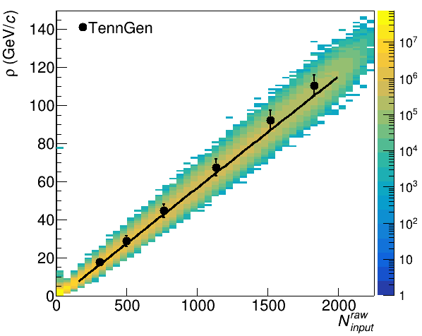
Figure 1 shows versus the reconstructed number of tracks for TennGen and Angantyr. These are fit to a straight line with the parameters given in Tab. 2 and compared to fits from ALICE:2012nbx. The multiplicity dependence is comparable to ALICE data in both models. Note that the data cover a wider range of multiplicities because TennGen only includes fixed multiplicities and Angantyr underestimates the multiplicity distribution by 5–10% Bierlich:2018xfw. This difference in the multiplicity means that neither model is directly comparable to the data. We therefore emphasize comparisons to expectations for a random background in the following sections.
| Slope | Intercept | |
|---|---|---|
| Angantyr | 0.0585 0.0002 | -1.67 0.09 |
| TennGen | 0.0610 0.0029 | -1.31 2.38 |
| ALICE data ALICE:2012nbx | 0.0623 0.0002 | -3.3 0.3 |
III.2 Distribution of
The soft background does not make jet measurements difficult because it is large, but because it fluctuates, which leads to large, jet-by-jet fluctuations. This smears the reconstructed jet energy. This smearing is corrected for in data and, because the background and its fluctuations are present in models which simulate the entire event, it also must be corrected for to make valid comparisons to Monte Carlo models which simulate the entire event. We therefore investigate the distribution of these background fluctuations and compare them to ALICE measurements of background fluctuations.
Two random cones with a radius are drawn within 0.5 for each event. The of all reconstructed charged hadrons in the cone are added and the background density estimated from jets found with the jet finder is subtracted to get
| (3) |
where . The distribution of is a measure of the fluctuations in the background.

Figure 2 shows the distribution of in 3 different sets of points: ALICE data in Pb+Pb collisions at = 2.76 TeV ALICE:2012nbx, TennGen, and Angantyr. The leading jet has been excluded from both the ALICE data and Angantyr. Even though TennGen uses ALICE single-particle spectra and , the distributions do not overlap. This is in part because TennGen uses the average multiplicity and does not include fluctuations in the number of particles, leading to a somewhat narrower distribution than the data. Furthermore, TennGen contains no hard processes, resonances, mini-jets or decays. Angantyr contains multiplicity fluctuations and the previously mentioned processes but underestimates the event multiplicity.
III.3 Width of the distribution
Understanding the width of fluctuations in the background is important for possible improvements in methods, since the width of the background fluctuations drives the uncertainties from unfolding. In ALICE:2012nbx, the width of the distribution is compared to predictions assuming only fluctuations in the number of particles in the random cone and their momenta and correlations in the distribution of background particles due to flow. There were small deviations between data and the predictions, but it is not possible to isolate the source of these deviations with studies of data alone. We compare our model to the same predictions.
The distribution of the sum of momenta from a random sample of particles is discussed in TANNENBAUM200129, where it is applied to distributions of transverse energy in events. These derivations were applied in ALICE:2012nbx to the problem of random cones. In TANNENBAUM200129, the single-particle spectrum is approximated as a gamma distribution
| (4) |
where and are constants and if is an integer. The -fold convolution of this distribution is itself another gamma distribution with a mean given by and standard deviation . The distribution in Fig. 2 can therefore be fit to a gamma distribution to extract the width.
When there are Poissonian fluctuations in the number of particles in the sample, the distribution is a sum of gamma distributions, with a standard deviation given by
| (5) |
For both TennGen with =0 and Angantyr, the distribution of the number of particles in the random cone were consistent with a Poissonian distribution. Appendix A.1 includes a detailed derivation of Eq. 5 and Appendix A.2 investigates how Eq. 5 would change if the spectrum were more complicated than a single gamma distribution.
The presence of hydrodynamic flow in Eq. 2 leads to non-Poissonian number fluctuations. If the fluctuations from each term are approximated as uncorrelated and constant as a function of momentum, the width is given by
| (6) |
In ALICE:2012nbx, only and terms were considered. These assumptions could be sources of deviations between Eq. 6 and the observed widths. In addition Eq. 6 assumes that the terms are independent of . For the calculations of Eq. 6 compared to TennGen in this analysis, the un-weighted average from TennGen is used. Note that in Eq. 5 and Eq. 6 is the number of particles in the random cone, not the charged particle multiplicity in the event. In Appendix A.3 we investigate the impact of flow in greater detail.
III.3.1 TennGen

Figure 3 shows in TennGen with =0 compared to Eq. 5 and with non-zero compared to Eq. 6. The predictions from Eq. 5 and Eq. 6 use , , and in TennGen. The slight deviations seen here are qualitatively consistent with ALICE:2012nbx, but the absence of any correlations other than flow makes the discrepancy easier to interpret in TennGen. The derivation of Eq. 5 assumed that the single particle spectra were a gamma distribution while TennGen uses a blast wave, which could explain the roughly 2% deviation between TennGen with =0 and Eq. 5. This indicates that the width is dependent on the shape of the spectrum. The derivation of Eq. 6 assumed that both the are independent of and that there are no correlations between number fluctuations due to flow, explaining the deviations as high as 6% between this prediction and TennGen with nonzero flow. The derivations in Appendices A.1 and A.2 confirm that these effects can explain the deviations from Eq. 5 and Eq. 6.
III.3.2 Angantyr
Figure 4 compares the widths in Angantyr with no jets excluded, the leading jet excluded, and the leading two jets excluded from the sample to Eq. 5. Leading jets are excluded by requiring a large separation between the axis of the random cone and the anti- jet axis, . The predictions from Eq. 5 use the , , and in Angantyr. The widths in Angantyr have an average difference of 12% with respect to what is predicted by Eq. 5 when no leading jets are removed. The discrepancy gets smaller when jets are excluded from the sample. The average differences are 4% and 3% when one or two leading jets are removed, respectively.
Figure 5 shows the widths in Pb+Pb collisions at = 2.76 TeV and Au+Au collisions at = 200 GeV with the two leading jets removed from the sample. The predictions from Eq. 5 use the , , and from Angantyr at each energy. The average difference from the prediction in Au+Au is 2%. The lower energy should have fewer jets than the higher energy, which could partially explain why the is closer to the prediction in Au+Au. Additional differences could be from the difference between the particle spectrum in Angantyr and a gamma distribution.
Figure 6 shows fits of the particle spectra from Pb+Pb collisions at = 2.76 TeV in data and in Angantyr to a gamma distribution. Since these are single particle spectra, it is not possible to remove particles from jets. The gamma distribution describes the data better than it describes Angantyr. This indicates that the deviations between Angantyr and predictions from Eq. 5 shown in Figure 4 may be largely due to the difference in the shapes of the spectra, as supported by the calculations in Appendix A.2.


III.4 Unfolding jets in heavy-ion collision Monte Carlo
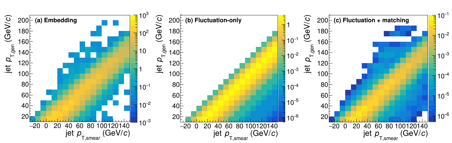
Experiments correct for the migration of jets from their correct momentum bin to another bin, which distorts the momentum, using a procedure called unfolding DAgostini:2010hil; Hocker:1995kb. In experiment, this smearing arises due to both detector effects and jet background fluctuations. Usually, a response matrix is determined from full simulation of the detector response to a jet. A simulated PYTHIA + collision may be embedded in data from a heavy ion collision in order to use a data-driven smearing due to fluctuations in the background; we construct a similar response matrix using a Pb+Pb collision from Angantyr and call this the “embedding response matrix”. Alternatively, a response matrix including both effects can be determined by multiplying two response matrices, one describing the detector response to a jet in + collision and one describing background fluctuations observed in the data ALICE:2015mjv. In the absence of detector effects, as is the case in these studies, the only effect is from background fluctuations; we construct a similar response matrix for Angantyr using the fluctuations in Fig. 2 and call this the “fluctuation-only response matrix”. We also construct a response matrix using a PYTHIA + event embedded in an Angantyr Pb+Pb event but only using the particles from the + event to determine the measured jet momentum, and then multiply this matrix by the background fluctuation response matrix. This should capture changes in the behavior of the jet finder in a heavy ion collision while still maintaining the assumption that the impact of changes in the behavior of the jet finder and fluctuations in the background can be factorized. We call this the “fluctuation plus matching response matrix.”
Two sets of jets are reconstructed, one containing only charged particles from the + event, which is considered the generated distribution, and another using all charged particles in either event, which is considered the smeared distribution. In order to build the response matrix, a match between the jets in the two sets is established by requiring a bijective match and where and are the differences in and between the generated and smeared jets. We do not include the impact of the finite single track reconstruction efficiency.
The response matrices are shown in Fig. 7. The fluctuation-only response matrix does not describe jets reconstructed well in the region where the reconstructed momenta is below the true momenta, which can be seen in the embedding response matrix, and it predicts a significant contribution from jets reconstructed well above their true momenta, which is not evident in the embedding response matrix. The fluctuation plus matching response matrix is also unable to capture this behavior.
In order to demonstrate closure, an unfolded distribution has to converge to the true distribution. We use only the jets in the combined Pb+Pb plus + event which were matched to a jet in the + event and unfold this transverse momentum spectrum using the different response matrices. We compare this to the true transverse momentum spectrum in PYTHIA + events. We use Bayesian unfolding implemented in the RooUnfold Adye:2011gm package. The singular value decomposition method was used as a cross-check and all results were consistent with those obtained with Bayesian unfolding.

The ratios of the unfolded spectra to the true distributions are shown in Fig. 8. The number of iterations in the Bayesian unfolding procedures is varied from 2 to 7. The results using the embedding response matrix converge quickly, with little change after the second iteration, and this procedure successfully recovers the true distribution to within around 4% . The results using the fluctuation-only response matrix change more and the difference between the results and the true distribution is about 5% below 110 GeV/, increasing to about 10% above that. The results from the fluctuation plus matching response matrix are comparable to those with the fluctuation-only response matrix.
The spectra unfolded using the fluctuation-only and the fluctuation plus matching response matrices are systematically lower than the true spectra. This could skew the interpretation of comparisons between models and data. This indicates that there is an interplay between background fluctuations and the behavior of the jet finder in a heavy ion environment, and that robust comparisons between data and full Monte Carlo models may require not just unfolding, but a response matrix created using embedding, just like the procedure for data analysis.
IV Discussion
Our first observation is that a large, fluctuating background uncorrelated with jet measurements is, indeed, present in Monte Carlos which simulate the full event, necessitating background subtraction in such models.
Other models, such as JEWEL Zapp:2008gi nominally give the user only the particles from signal jets with only some ambiguity as to which particles from the medium were influenced by the jet. This ambiguity can be approached by looking at the two extremes, when only particles from the hard parton shower are included and when medium particles which have interacted with the jet are included KunnawalkamElayavalli:2016lzw.
That works well if the only possible uncertainty is theoretical. However, the field has made incomplete assumptions about the background for jet measurements in the past, for instance omitting from the background for dihadron correlations, leading to several erroneous observations Connors:2017ptx. Biases, or even mistakes, in measurements due to incomplete assumptions about the background subtraction are possible. We therefore advocate following the philosophy of RIVET Bierlich:2020wms: the exact same strategy should be used in both the analysis and the Monte Carlo model, to the extent possible, in order to ensure that the comparison between data and the model is valid. In practice, this means that the background subtraction should be implemented in Monte Carlo. In dihadron correlations, this would have resulted in valid comparisons between models and data, even though the result would be more sensitive to the soft background than was intended in the measurement. For models such as JEWEL, which nominally contain only or mostly particles directly from the jet signal, aspects of the background subtraction could still be applied, particularly when they might impose a bias in the measurement. For example, reflection about for the background subtraction Chatrchyan:2014ava; Chatrchyan:2012gw could be implemented in JEWEL.
For Monte Carlo models which simulate the full event, such as Angantyr, this means that the exact same background subtraction method should be applied to the model as is used in data, including the corrections for fluctuations. Background fluctuations are significantly different in models and in data, so it is not sufficient for comparisons to use experimental observations of the fluctuations or an experimental response matrix. This poses some complications for uncorrected measurements, even if the response matrix is provided with the measurement, as the fluctuations will be different in the model and the data. The sensitivity of the shape of the background to subtle differences in the shape of the spectrum and the details of correlations between particles in background poses particular problems for comparisons between data and models. It implies that the corrections for the background fluctuations must be done separately for each model, using a method consistent with that used in data. Moreover, we find that it is necessary to unfold using a response matrix constructed in the same way as in the measurement.
V Conclusions
While our studies broadly support the conclusions in ALICE:2012nbx that the background fluctuations are dominated by random combinations of particles, we find that this width is sensitive to both details of the hydrodynamical background and the shape of the single particle momentum spectrum. These effects are less than 6% for TennGen, a data-driven random background generator, and around 13% in PYTHIA Angantyr depending on how many jets are removed from the events.
As measurements of jets in heavy-ion collisions reach higher precision, it is important to make sure that models are comparable to data. Some of the details of flow correlations would be difficult to fully describe in background subtraction methods. Area-based subtraction techniques such as those used by ALICE with a data-driven determination of the fluctuations Abelev:2013kqa; ALICE:2015mjv and the -reflection method used by CMS Chatrchyan:2014ava; Chatrchyan:2012gw should be robust to these effects.
It is less clear how these subtle effects in the width of fluctuations in the background would be incorporated into mixed events Adamczyk:2017yhe or impacted by the iterative subtraction techniques used by CMS Khachatryan:2016jfl and ATLAS Aad:2012vca. Many models, such as Angantyr, may not accurately reproduce the background in heavy ion collisions. Implementation of the full experimental method in model calculations, using tools such as Rivet, is essential for robust and meaningful comparisons between models and data.
We note that there are models which do not attempt to simulate the full event, such as JEWEL Zapp:2008gi, as well as models where it is possible to separate jet “signal.” This may reduce the direct sensitivity to background models, but it adds an additional theoretical uncertainty, since arbitrary distinctions between “signal” and “background” must be made. This may be less problematic for certain observables, particularly those less sensitive to soft radiation; however, it is precisely those observables which are likely to be most interesting for studies of partonic energy loss. We therefore urge care in comparisons between data and models, reproducing as many parts of the experimental method as possible.
VI Acknowledgements
We are grateful to Christian Klein-Bösing, Marco van Leeuwen, Leif Lönnblad, Mike Tannenbaum, and Gary Westfall for productive discussions and Alexandre Shabetai and Ejiro Umaka for feedback on the manuscript. This work was supported in part by funding from the Division of Nuclear Physics of the U.S. Department of Energy under Grant No. DE-FG02-96ER40982 and from the National Science Foundation under Grant No. OAC-1550300. We also acknowledge support from the UTK and ORNL Joint Institute for Computational Sciences Advanced Computing Facility.
References
- [1] K. Adcox et al. Formation of dense partonic matter in relativistic nucleus nucleus collisions at RHIC: Experimental evaluation by the PHENIX collaboration. Nucl. Phys., A757:184–283, 2005.
- [2] John Adams et al. Experimental and theoretical challenges in the search for the quark gluon plasma: The STAR collaboration’s critical assessment of the evidence from RHIC collisions. Nucl. Phys., A757:102–183, 2005.
- [3] B. B. Back et al. The PHOBOS perspective on discoveries at RHIC. Nucl. Phys., A757:28–101, 2005.
- [4] I. Arsene et al. Quark Gluon Plasma an Color Glass Condensate at RHIC? The perspective from the BRAHMS experiment. Nucl. Phys., A757:1–27, 2005.
- [5] Megan Connors, Christine Nattrass, Rosi Reed, and Sevil Salur. Jet measurements in heavy ion physics. Rev. Mod. Phys., 90:025005, 2018.
- [6] Karen M. Burke et al. Extracting the jet transport coefficient from jet quenching in high-energy heavy-ion collisions. Phys.Rev., C90(1):014909, 2014.
- [7] S. Cao et al. Determining the jet transport coefficient q from inclusive hadron suppression measurements using Bayesian parameter estimation. Phys. Rev. C, 104(2):024905, 2021.
- [8] L. Adamczyk et al. Measurements of jet quenching with semi-inclusive hadron+jet distributions in Au+Au collisions at = 200 GeV. Phys. Rev., C96(2):024905, 2017.
- [9] Betty Abelev et al. Measurement of Event Background Fluctuations for Charged Particle Jet Reconstruction in Pb-Pb collisions at TeV. JHEP, 03:053, 2012.
- [10] Charles Hughes and Christine Nattrass. TennGen Source Code and Documentation. https://github.com/chughes90/TennGen. Accessed: 2020-05-05.
- [11] Christian Bierlich, Gösta Gustafson, Leif Lönnblad, and Harsh Shah. The Angantyr model for Heavy-Ion Collisions in PYTHIA8. JHEP, 10:134, 2018.
- [12] Torbjorn Sjostrand, Stephen Mrenna, and Peter Z. Skands. PYTHIA 6.4 Physics and Manual. JHEP, 05:026, 2006.
- [13] Betty Abelev et al. Centrality Dependence of Charged Particle Production at Large Transverse Momentum in Pb–Pb Collisions at TeV. Phys. Lett., B720:52–62, 2013.
- [14] O. Ristea, A. Jipa, C. Ristea, T. Esanu, M. Calin, A. Barzu, A. Scurtu, and I. Abu-Quoad. Study of the freeze-out process in heavy ion collisions at relativistic energies. J. Phys. Conf. Ser., 420:012041, 2013.
- [15] Ekkard Schnedermann, Josef Sollfrank, and Ulrich W. Heinz. Thermal phenomenology of hadrons from 200-A/GeV S+S collisions. Phys. Rev. C, 48:2462–2475, 1993.
- [16] Betty Abelev et al. Centrality dependence of , K, p production in Pb-Pb collisions at = 2.76 TeV. Phys. Rev., C88:044910, 2013.
- [17] Kenneth Aamodt et al. Centrality dependence of the charged-particle multiplicity density at mid-rapidity in Pb-Pb collisions at = 2.76 TeV. Phys. Rev. Lett., 106(CERN-PH-EP-2010-071. CERN-PH-EP-2010-071):032301. 14 p, Dec 2010.
- [18] Georges Aad et al. Measurement of event-plane correlations in TeV lead-lead collisions with the ATLAS detector. Phys. Rev. C, 90(2):024905, 2014.
- [19] Jaroslav Adam et al. Higher harmonic flow coefficients of identified hadrons in Pb-Pb collisions at = 2.76 TeV. JHEP, 09:164, 2016.
- [20] Matthew Luzum and Jean-Yves Ollitrault. Directed flow at midrapidity in heavy-ion collisions. Phys. Rev. Lett., 106:102301, 2011.
- [21] Georges Aad et al. Measurement of the azimuthal anisotropy for charged particle production in TeV lead-lead collisions with the ATLAS detector. Phys. Rev., C86:014907, 2012.
- [22] Ekaterina Retinskaya, Matthew Luzum, and Jean-Yves Ollitrault. Directed flow at midrapidity in TeV Pb+Pb collisions. Phys. Rev. Lett., 108:252302, 2012.
- [23] Andy Buckley, Jonathan Butterworth, David Grellscheid, Hendrik Hoeth, Leif Lonnblad, James Monk, Holger Schulz, and Frank Siegert. Rivet user manual. Comput. Phys. Commun., 184:2803–2819, 2013.
- [24] P Cortese et al. ALICE technical design report on forward detectors: FMD, T0 and V0. 9 2004.
- [25] Betty Bezverkhny Abelev et al. Performance of the ALICE Experiment at the CERN LHC. Int. J. Mod. Phys. A, 29:1430044, 2014.
- [26] Matteo Cacciari, Gavin P. Salam, and Gregory Soyez. Fastjet user manual. The European Physical Journal C, 72(3), Mar 2012.
- [27] Matteo Cacciari and Gavin P. Salam. Pileup subtraction using jet areas. Phys. Lett. B, 659:119–126, 2008.
- [28] M.J. Tannenbaum. The distribution function of the event-by-event average pt for statistically independent emission. Physics Letters B, 498(1):29 – 34, 2001.
- [29] G. D’Agostini. Improved iterative Bayesian unfolding. In Alliance Workshop on Unfolding and Data Correction, 10 2010.
- [30] Andreas Hocker and Vakhtang Kartvelishvili. SVD approach to data unfolding. Nucl. Instrum. Meth. A, 372:469–481, 1996.
- [31] Jaroslav Adam et al. Measurement of jet suppression in central Pb-Pb collisions at = 2.76 TeV. Phys. Lett. B, 746:1–14, 2015.
- [32] Tim Adye. Unfolding algorithms and tests using RooUnfold. In PHYSTAT 2011, pages 313–318, Geneva, 2011. CERN.
- [33] Korinna Zapp, Gunnar Ingelman, Johan Rathsman, Johanna Stachel, and Urs Achim Wiedemann. A Monte Carlo Model for ’Jet Quenching’. Eur. Phys. J. C, 60:617–632, 2009.
- [34] Raghav Kunnawalkam Elayavalli and Korinna Christine Zapp. Medium Recoils and background subtraction in JEWEL. Nucl. Part. Phys. Proc., 289-290:368–371, 2017.
- [35] Christian Bierlich et al. Confronting experimental data with heavy-ion models: RIVET for heavy ions. Eur. Phys. J. C, 80(5):485, 2020.
- [36] Serguei Chatrchyan et al. Measurement of jet fragmentation in PbPb and pp collisions at TeV. Phys.Rev., C90(2):024908, 2014.
- [37] Serguei Chatrchyan et al. Measurement of jet fragmentation into charged particles in and PbPb collisions at TeV. JHEP, 1210:087, 2012.
- [38] B. Abelev et al. Measurement of charged jet suppression in Pb-Pb collisions at = 2.76 TeV. JHEP, 03:013, 2014.
- [39] Vardan Khachatryan et al. Measurement of inclusive jet cross sections in and PbPb collisions at 2.76 TeV. Phys. Rev., C96(1):015202, 2017.
- [40] Georges Aad et al. Measurement of the jet radius and transverse momentum dependence of inclusive jet suppression in lead-lead collisions at = 2.76 TeV with the ATLAS detector. Phys.Lett., B719:220–241, 2013.
*
Appendix A Derivations
A.1 Mean and width of the sum of particles drawn from a distribution
The derivation of the distribution of energies in [28] and the associated widths in [9] assumed a spectrum of the form
| (7) |
where is the number of particles, is the transverse momentum, and , , and are constants. The normalized probability distribution, , for the probability of a single random particle drawn from the distribution having a momentum takes the same form, with . As in [28], it is convenient to parametrize 7 in terms of the mean (b = ) and the variance (c = ):
| (8) |
It can be shown that the parameters and are in fact the mean and standard of deviation of 8:
| (9) | |||
| (10) |
The distribution of the sum of the momenta of two particles is given by the convolution where is 8:
| (11) |
This is repeated each time an additional particle is added, where each iteration is given by
| (12) |
where is the number of particles. The distribution of the total in the sample, , for particles drawn from this distribution is given by
| (13) |
with a corresponding mean in total cone given by
| (14) |
and variance
| (15) |
The total width of fluctuations of the sum of in a random cone is the quadrature sum of the Poissonian fluctuations in the number of particles in the random cone and the width of the n-fold convolution 15
| (16) |
where is the number of particles in the cone, is the mean of the single-particle distribution, and is the standard deviation of the of the single-particle distribution. Equation 16 is the same as Equation 3 in [13].
A.2 Deviations from a distribution
We note that the for integer form a complete set and we therefore can write an arbitrary spectral shape as
| (17) |
The prescription in Appendix Sec. A.1, in principle, also works for an arbitrary case such as this. Since a single term is shown in [9] to work well, we assume a form
| (18) |
where , , , , and are small and is much smaller than . Since the measured spectra are approximately a gamma distribution, this should provide a realistic quantification of deviations from a perfect gamma distribution. Taking into account an explicit normalization [such that the integral of 18 over all is 1], the mean of 18 is given by
| (19) |
and the variance is given by
| (20) |
Following the procedure laid out in Appendix A.1, we find the -fold convolution of 18. We do this using Laplace transforms, , and induction. The first convolution gives
| (21) |
The 2nd convolution gives:
| (22) |
By induction the n convolution is
| (23) |
The variance of 23 is
| (24) |
When combined with the Poissonian fluctuations in the number of particles in the cone, this can gives the width of the fluctuations for the sum of momentum in the cone as a function of particles in the cone:
| (25) |
This expression is difficult to simplify so that the impact of deviations from a Gamma distribution can be interpreted easily. Instead we use realistic numbers and show the impact in Fig. 9. Deviations from a single gamma distribution always increase the width, with the deviations increasing monotonically from that of a single gamma distribution. Thus we see that realistic deviations from a gamma distribution increase the width of the distribution of momenta in random cones.

In addition, we constructed gamma distributions with the same mean and standard deviation as the spectra in Angantyr and TennGen for Pb+Pb events at = 2.76 TeV. We drew several samples of the average number of particles observed in random cones for each generator and added up the total momentum. The track momentum distributions and the distribution of the total momenta are given in Fig. 10 and the properties of these distributions are given in Tab. 3. This exercise isolates the impact of the shape of the spectra alone. The shifts in the mean of the sums of all momenta are small. The shift in the standard deviation of the sum of all momenta from the true distribution to the gamma distribution is small for both, but larger for Angantyr. This also demonstrates that the shapes of the spectra are important for describing fluctuations in the background.
| (GeV/) | (GeV/) | ||
|---|---|---|---|
| Angantyr | 58 | 37.54 0.02 | 6.29 0.01 |
| Angantyr | 58 | 36.12 0.02 | 6.12 0.01 |
| TennGen | 52 | 35.68 0.02 | 6.12 0.01 |
| TennGen | 52 | 35.70 0.01 | 6.11 0.01 |


A.3 Including azimuthal anisotropy
We consider the azimuthal anisotropy due to and show that this is a special case of that derived in Sec. A.2. The standard expression of azimuthal anisotropy in a heavy ion collision is
| (26) |
where is a normalization factor, is the azimuthal angle of a particle’s momentum vector, is the azimuthal position of the th order event plane, and the are the th order azimuthal anisotropies. Without loss of generality, we can express the momentum dependence of the with a Taylor expansion
| (27) |
where the are constants so that Eq. 26 can be rewritten as
| (28) |
The dominant can be chosen so that this can be rewritten in the form of Eq. 17. If only the first term is kept, corresponding to constant , the momentum and azimuthal dependencies factorize. The analysis in Appendix A.1 can be applied to the momentum dependence. The mean is given by
| (29) |
The average does not change because the average over all azimuthal angles is one. The standard deviation is given by
| (30) |
This also does not change. The change in standard deviation due to in Eq. 6 is entirely because of the change in the number of particles. However, including a single momentum dependent term in the in Eq. 28 increases deviations of from a single gamma distribution, increasing the width. Since the are momentum-dependent, any realistic will increase the width.