A robust algorithm for explaining unreliable machine learning survival models using the Kolmogorov-Smirnov bounds
Abstract
A new robust algorithm based of the explanation method SurvLIME called SurvLIME-KS is proposed for explaining machine learning survival models. The algorithm is developed to ensure robustness to cases of a small amount of training data or outliers of survival data. The first idea behind SurvLIME-KS is to apply the Cox proportional hazards model to approximate the black-box survival model at the local area around a test example due to the linear relationship of covariates in the model. The second idea is to incorporate the well-known Kolmogorov-Smirnov bounds for constructing sets of predicted cumulative hazard functions. As a result, the robust maximin strategy is used, which aims to minimize the average distance between cumulative hazard functions of the explained black-box model and of the approximating Cox model, and to maximize the distance over all CHFs in the interval produced by the Kolmogorov-Smirnov bounds. The maximin optimization problem is reduced to the quadratic program. Various numerical experiments with synthetic and real datasets demonstrate the SurvLIME-KS efficiency.
Keywords: interpretable model, explainable AI, survival analysis, censored data, linear programming, the Cox model, Kolmogorov-Smirnov bounds.
1 Introduction
A rapid and significant success in applying machine learning models to a wide range of applications, especially to medicine [31], meets a problem of understanding results provided by the models, for example, a doctor has to have an explanation of a stated diagnosis in order to choose a corresponding treatment. However, many models are black-box, i.e., their inputs and outcomes may be known for users, but it is not clear what information in the input data makes them actually arrive at their decisions. Therefore, explanations of the machine learning model prediction can help machine users or machine learning experts to understand the obtained results, and the model explainability becomes to be an important component of machine learning and even a key factor of decision making [8, 26, 51, 54].
One of the groups of explanation methods consists of the so-called local methods which derive explanation locally around a test example. They aim to assign to every feature of the test example some number quantified its impact on the prediction in order to explain the contribution of individual input features. One of the first local explanation methods is the Local Interpretable Model-agnostic Explanations (LIME) [59], which uses simple and easily understandable linear models to locally approximate the predictions of black-box models. According to LIME, the explanation may be derived locally from a set of synthetic examples generated randomly in the neighborhood of the example. A thorough theoretical analysis of LIME is given by Garreau and Luxburg [24] where the authors note that LIME is flexible to provide explanations for different data types, including text and image data.
Among a large variety of machine learning models, we select the models which try to solve a fundamental problem of survival analysis to understand the relationship between the covariates and the distribution of survival times to events of interest. Survival analysis is an important field of statistics which aims at predicting the time to events of interest, and it can simultaneously model event data and censored data [32]. By taking into account the importance of the survival analysis tasks, a lot of machine learning survival models have been developed [42, 81, 91]. One of the main peculiarities of the survival models is that their outcomes are functions (the survival function, the hazard function, the cumulative hazard function, etc.) as predictions instead of points.
A popular model, which establishes the relationship between the covariates and the distribution of survival times, is the semi-parametric Cox proportional hazards model [18]. The model assumes that a patient’s log-risk of failure is a linear combination of the example covariates. This is a very important property of the Cox model, which can be used below in explanation models.
Taking into account the need to explain the machine learning black-box survival models, Kovalev et al. [41] proposed an explanation method called SurvLIME, which deals with censored data and can be regarded as an extension of LIME on the case of survival data. The basic idea behind SurvLIME is to apply the Cox model to approximate the black-box survival model at a local area around a test example. The Cox model is chosen due to its assumption of the linear combination of covariates. This assumption implies that coefficients of the covariates can be viewed as quantitative impacts on the prediction.
The main problem of using SurvLIME is a lack of robustness to cases of a small amount of training data or outliers of survival data. There are many machine learning methods which try to cope with this problem. One of the ways to implement the robust models is to incorporate the imprecise probability or statistical inference models [78], which use sets of probability distributions on data instead of a single distribution. The robust models based on imprecise probabilities use the maximin strategy, which can be interpreted as an insurance against the worst case because it aims at minimizing the expected loss in the least favorable case [61]. Robust models have been widely exploited in regression and classification problems due to the opportunity to avoid some strong assumptions underlying the standard classification models [87]. The imprecise probability models have been applied also to survival models (see, for example, [46]). However, we have to point out that the above robust models have been incorporated into the machine learning models themselves, but not to their explanations. Therefore, our aim is to develop an algorithm for explaining the machine learning survival models, which could be robust to the small amount of training data and to outliers in the training or testing sets.
Pursuing this goal, we propose a robust explanation algorithm which is called as SurvLIME-KS and can be regarded as a modification of SurvLIME. It uses the well-known Kolmogorov-Smirnov (KS) bounds [36] for the predicted cumulative hazard function (CHF). KS bounds make no distributional assumptions and can be considered in the framework of the imprecise statistical models. KS bounds have been used to realize robust machine learning models (see, for example, [71]). The following ideas are the basis for SurvLIME-KS:
- 1.
SurvLIME is used as a basis for the proposed robust algorithm. It generates many points at a local area around a test example, and the CHF is predicted for every generated example by the black-box machine learning model which has to be explained.
- 2.
Every CHF predicted by the black-box machine learning model is transformed to a cumulative distribution function for which KS bounds are determined in accordance with the predefined confidence probability. In order to construct bounds for the CHF, the inverse transformation is carried out.
- 3.
A maximin optimization problem is stated and solved for getting optimal coefficients of the approximating Cox model, where the minimum is defined for the average distance between logarithms of CHFs produced by the explained black-box model and by the approximating Cox model, it is taken over coefficients of the approximating Cox model, the maximum is taken over logarithms of all CHFs restricted by the obtained bounds. The distance between two functions is based on -norm. Chebyshev distance metrics is used because it has an inferior computational cost due to its simple formulation.
- 4.
The problem is reduced to a standard quadratic optimization problem with linear constraints.
Many numerical experiments illustrate SurvLIME-KS under different conditions of training data. It is shown on synthetic and real data that the algorithm provides outperforming results for small data and under outliers.
The paper is organized as follows. Related work is in Section 2. Basic concepts of survival analysis and the Cox model are given in Section 3. A brief description of the method LIME is provided in Section 4. An introduction to KS bounds is given in Section 5. Section 6 provides a description of the proposed algorithm SurvLIME-KS and its basic ideas. A derivation of the optimization problem for determining important features under condition of the lack of KS bounds, i.e., when the predicted CHFs are precise, can be found in Section 7. Questions of incorporating KS bounds into the explanation method and reducing the maximin optimization problem to the quadratic programming problem are considered in Section 8. Numerical experiments with synthetic data and real data are provided in Section 9. Concluding remarks can be found in Section 10.
2 Related work
Local explanation methods. Due to importance of the machine learning model explanation in many applications, a lot of methods have been proposed to locally explain black-box models. Following the original LIME [59], a lot of its modifications have been developed due to a simple nice idea underlying the method to construct a linear approximating model in a local area around a test example. These modifications are ALIME [63], NormLIME [6], DLIME [88], Anchor LIME [60], LIME-SUP [33], LIME-Aleph [56], GraphLIME [34], SurvLIME [41]. Another explanation method, which is based on linear approximation, is the SHAP [45, 65], which takes a game-theoretic approach for optimizing a regression loss function based on Shapley values.
In order to get intuitive and human-friendly explanations, another explanation technique called as counterfactual explanations [77] was developed by several authors [25, 30, 43, 75]. The corresponding methods tell us what to do in order to achieve a desired outcome. Counterfactual modifications of the LIME were proposed by Ramon et al. [57] and White and Garcez [82].
Another important group of explanation methods is based on perturbation techniques [22, 23, 55, 76], which are also used in LIME. The basic idea behind the perturbation techniques is that contribution of a feature can be determined by measuring how a prediction score changes when the feature is altered [20]. Perturbation techniques can be applied to a black-box model without any need to access the internal structure of the model. However, the corresponding methods are computationally complex when samples are of the high dimensionality.
A lot of explanation methods, their analysis and critical review can be found in survey papers [5, 7, 14, 26, 62, 86].
Most explanation methods deal with the point-valued results produced by explainable black-box models, for example, with classes of examples. In contrast to these models, outcomes of survival models are function, for example, SFs or CHFs. It follows that LIME should be extended on the case of models with functional outcomes, in particular, with survival models. An example of such the extended model is SurvLIME [41].
Machine learning models in survival analysis. Wang et al. [81] provided a comprehensive review of the machine learning models dealing with survival analysis problems. The most powerful and popular method for dealing with survival data is the Cox model [18]. Following this model, a lot of its modifications have been developed in order to relax some strong assumption underlying the Cox model. In order to take into account the high dimensionality of survival data and to solve the feature selection problem with these data, Tibshirani [66] presented a modification based on the Lasso method. Similar Lasso modifications, for example, the adaptive Lasso, were also proposed by several authors [40, 84, 90]. The next extension of the Cox model is a set of SVM modifications [39, 83]. Various architectures of neural networks, starting from a simple network [21] proposed to relax the linear relationship assumption in the Cox model, have been developed [27, 38, 58, 92] to solve prediction problems in the framework of survival analysis. In spite of many powerful machine learning approaches for solving the survival problems, the most efficient and popular tool for survival analysis under condition of small survival data is the extension of the standard random forest [13] called the random survival forest (RSF) [35, 50, 80, 85].
Most of the above models dealing with survival data can be regarded as black-box models and should be explained. However, only the Cox model has a simple explanation due to its linear relationship between covariates. Therefore, it can be used to approximate more powerful models, including survival deep neural networks and random survival forests, in order to explain predictions of these models.
Imprecise probabilities in classification and regression. There are a lot of results devoted to application of the imprecise probability models [79] to classification and regression problems. Several authors [17, 89] proposed “imprecise” classifiers that are reliable even in the presence of small sample sizes and missing values due to use of imprecise statistical models. Modifications of SVM and random forests on the basis of incorporating the imprecise models have been presented in papers [67, 68, 69].
Robust classification and regression models using the Kolmogorov-Smirnov bounds have been applied to classification [71] and regression problems [70, 74] to take into account the lack of sufficient training data and for constructing accurate classification or regression models. One of the first ideas of applying imprecise probability models to classification decision trees was presented in [4], where probabilities of classes at decision tree leaves are estimated by using an imprecise model. Following this work, several papers devoted to applications of imprecise probabilities to decision trees and random forests were proposed [1, 2, 3, 47, 53], where the authors developed new splitting criteria taking into account imprecision of training data and noisy data. Imprecise probabilities have also been used in classification problems in [19, 49, 52].
Imprecise probabilities in survival analysis. One of the ways for getting robust survival models is to incorporate imprecise probability models into survival analysis. Mangili et al. [46] proposed a robust estimation of survival functions from right censored data by introducing a robust Dirichlet process. In this paper, special bounds for SFs and the corresponding survival curve estimator are presented.
Another approach illustrating how the imprecise Dirichlet model can be used to determine upper and lower values on the survival function was proposed in [11, 12]. Application of the imprecise Dirichlet model to survival data was also studied by Coolen [15]. Coolen and Yan [16] considered a generalization of Hill’s assumption, which is used for prediction in case of extremely vague prior knowledge about the underlying distribution, for dealing with right-censored observations. Modifications of random survival forests by assigning weights to decision trees in a way that allows us to control the imprecision and to implement the robust strategy of decision making are proposed in [72, 73].
In spite of many papers devoted to the robust machine learning models mentioned above, there are no methods of the robust local explanation of survival models. Therefore, the proposed incorporating KS bounds into SurvLIME can be regarded as the first robust explanation method of the survival model predictions.
3 Some elements of survival analysis
3.1 Basic concepts
In survival analysis, an example (patient) is represented by a triplet , where is the vector of the patient parameters (characteristics) or the vector of the example features; is time to event of the example. If the event of interest is observed, corresponds to the time between baseline time and the time of event happening, in this case , and we have an uncensored observation. If the example event is not observed and its time to event is greater than the observation time, corresponds to the time between baseline time and end of the observation, and the event indicator is , and we have a censored observation. Suppose a training set consists of triplets , . The goal of survival analysis is to estimate the time to the event of interest for a new example (patient) with feature vector denoted by by using the training set .
The survival and hazard functions are key concepts in survival analysis for describing the distribution of event times. The survival function (SF) denoted by as a function of time is the probability of surviving up to that time, i.e., . The hazard function is the rate of event at time given that no event occurred before time , i.e., , where is the density function of the event of interest. The hazard rate is defined as
| (1) |
Another important concept is the CHF , which is defined as the integral of the hazard function and can be interpreted as the probability of an event at time given survival until time , i.e.,
| (2) |
The SF can be expressed through the CHF as .
To compare the survival models, the C-index proposed by Harrell et al. [29] is used. It estimates how good the model is at ranking survival times. It estimates the probability that, in a randomly selected pair of examples, the example that fails first had a worst predicted outcome. In fact, this is the probability that the event times of a pair of examples are correctly ranking.
3.2 The Cox model
Let us consider main concepts of the Cox proportional hazards model, [32]. According to the model, the hazard function at time given predictor values is defined as
| (3) |
Here is a baseline hazard function which does not depend on the vector and the vector ; is the covariate effect or the risk function; is an unknown vector of regression coefficients or parameters. It can be seen from the above expression for the hazard function that the reparametrization is used in the Cox model. The function in the model is linear, i.e.,
| (4) |
In the framework of the Cox model, the survival function is computed as
| (5) |
Here is the cumulative baseline hazard function; is the baseline survival function. It is important to note that functions and do not depend on and .
The partial likelihood in this case is defined as follows:
| (6) |
Here is the set of patients who are at risk at time . The term “at risk at time ” means patients who die at time or later.
4 LIME
Let us briefly consider the original LIME [59]. It is an explanation framework for the decision of many machine learning classifiers. The method proposes to approximate a black-box explainable model denoted as with a simple function in the vicinity of the point of interest , whose prediction by means of has to be explained, under condition that the approximation function belongs to a set of explanation models , for example, linear models. In order to construct the function in accordance with LIME, a new dataset consisting of perturbed samples is generated, and predictions corresponding to the perturbed samples are obtained by means of the explained model. New samples are assigned by weights in accordance with their proximity to the point of interest by using a distance metric, for example, the Euclidean distance.
An explanation (local surrogate) model is trained on new generated samples by solving the following optimization problem:
| (7) |
Here is a loss function, for example, mean squared error, which measures how the explanation is close to the prediction of the explainable model; is the model complexity.
Finally, LIME provides a local linear model which explains the prediction by analyzing its coefficients.
5 Kolmogorov-Smirnov bounds
One of the ways for taking into account the amount of statistical data and for constructing bounds for the set of probability distributions is using the Kolmogorov-Smirnov confidence limits for the empirical cumulative distribution function constructed on the basis of observations.
Suppose that function is a true probability distribution function of points from the training set. It is assumed that is unknown. If the training set consists of examples, then a critical value of the test statistic can be chosen such that a band of width around will entirely contain with probability , which is to be interpreted as a confidence statement in the frequentist statistical framework. In other words, we can write , where the quantity is called the Kolmogorov-Smirnov statistic. Denote the -quantile of the Kolmogorov distribution by . The ways for computing for given and as well as the values of can be found in the book [36]. In particular, according to [36], a good approximation for the test statistic for is given by
| (8) |
For another approximation can be used [36]:
| (9) |
Taking into account that the bounds are cumulative distribution functions, we write the following bounds and for some unknown distribution function :
| (10) |
where
| (11) |
| (12) |
It can be seen from the above inequality that the left tail of the upper probability distribution is . The right tail of the lower probability distribution is . The corresponding jump is located at boundary points of the sample space far from all data points (see [70] for details).
It is also important to note that KS bounds depend on the number of training examples . This implies that these bounds can be applied to the robust explanation of the survival machine learning model predictions. The bounds allow us to develop new explanation models which take into account the lack of sufficient training data.
6 A sketch of SurvLIME-KS
SurvLIME-KS can be regarded as an extension of SurvLIME. Therefore, the first part of the sketch is devoted to SurvLIME. The second part is its extension.
Given a training set and a black-box model which produces an output in the form of the CHF for every new example . An idea behind SurvLIME is to approximate the output of the black-box model by means of the Cox model with the CHF denoted as for the same input example , where parameters are unknown a priori. This approximation allows us to get the coefficients of the approximating Cox model, whose values can be regarded as quantitative impacts on the prediction . The largest coefficients indicate the corresponding important features.
Optimal coefficients make the distance between CHFs and for the example as small as possible. Similarly to LIME, we consider many nearest examples generated in a local area around . For every generated , the CHF of the black-box model is predicted. By taking into account generated points and the corresponding CHFs , optimal values of minimize the weighted average distance between every pair of CHFs and over all points . Weight is assigned to the distance between points and in accordance with its value. In particular, smaller distances between and produce larger weights of distances between CHFs.
The distance metric between CHFs and defines the corresponding optimization problem for computing optimal coefficients . One of the possible ways is to apply -norms as a measure of a distance between two function. However, the direct use of -norms for defining distances between CHFs and may lead to extremely complex optimization problems. Therefore, SurvLIME [41] uses the -norm applied to logarithms of CHFs and , which leads to a convex optimization problem.
In contrast to SurvLIME, SurvLIME-KS uses the -norm as a distance between logarithms of CHFs and . It leads to a simpler optimization problem for computing the vector .
The first idea behind the SurvLIME-KS implementation is to define bounds for CHFs provided by the black-box model and their logarithms for all generated points . The logarithm is taken to simplify the optimization problem. The second idea is to extend the minimization problem for computing coefficients on a maximin optimization problem, where the maximum is taken over all logarithms of CHFs restricted by the defined bounds. The problem is solved by representing the minimization problem by the dual one. As a result, we get the maximization problem over logarithms of CHFs and coefficients . By adding the regularization term in the form of the quadratic norm, we get the standard quadratic optimization problem with linear constraints.
Fig. 1 illustrates the explanation algorithm. It can be seen from Fig. 1 that a set of examples are fed to the black-box survival model, which produces a set of CHFs . Simultaneously, we write CHFs , , as functions of coefficients for all generated examples. Then for every obtained CHF , the lower and upper bounds are introduced by using Kolmogorov-Smirnov bounds. The maximin optimization problem is written with the objective function which maximizes minimal weighted average distance between logarithms of CHFs and from a set of functions restricted by boundary functions and . Optimal values of coefficients is the solution to the problem.

7 -norm and the first part of SurvLIME-KS
In accordance with the sketch of the algorithm, points , , are generated in a local area around . Let us find the distances between CHFs provided by the black-box model for generated points , , and the CHF provided by the approximating Cox model for point . Before deriving the distances, we introduce some notations and conditions.
Let be the distinct times to event of interest from the set , where and . The black-box model maps the feature vectors into piecewise linear CHFs such that for all and . Let us introduce the time in order to restrict the function , where is a very small positive number. Let and divide it into subsets such that ; , , ; , .
Since the CHF is piecewise constant, then it can be written as
| (13) |
under additional condition , where is a small positive number. Here is a part of the CHF in interval , is the indicator function which takes value if , and otherwise.
It is important that does not depend on and is constant in interval . The last condition will be necessary below in order to deal with logarithms of the CHFs.
Let be a monotone function. Then there holds
| (14) |
The same expressions can be written for the CHF provided by the Cox model
| (15) |
The introduced condition allows us to use logarithms. Therefore, the distance between two CHFs is replaced with the distance between logarithms of the corresponding CHFs for the optimization problem. Let and be logarithms of and , respectively. Here is a generated point in a local area around . The difference between functions and can be written as follows:
| (16) |
Generally, the -norm can be used to write the distance between and . However, we consider the -norm or the Chebyshev distance because it leads to a maximin optimization problem which is rather simple from computational point of view and can be solved in a reasonable time. The -norm is a measure of the approximation quality, which is defined as the maximum of the absolute values or the maximum deviation between the function being approximated and the approximating function. Several authors [48, 64] pointed out that minimization is not robust to outliers, i.e., minimization may fit the outliers and not the good data. However, this disadvantage can be compensated by the introduce imprecision.
The distance between and is defined as
| (17) |
Hence, the optimization problem for computing is
| (18) |
Let us introduce the optimization variables
| (19) |
They are restricted as follows:
| (20) |
Every above constraint can be represented as the following pair of constraints:
| (21) |
| (22) |
Let us denote for short. Since the function is for all , and it is constant for all , then the last constraints can be rewritten as
| (26) |
| (27) |
The term does not depend on . Hence, the constraints can be reduced to the following simple constraints:
| (28) |
| (29) |
where
| (30) |
8 Kolmogorov-Smirnov bounds for robustifying explanations
Let us consider how to take into account the fact that the black-box model provides unreliable and inaccurate results due to a restricted number of training data or outliers. Let us return to the CHF representation (13) under condition considered above. We also assume that . Let us introduce the following function:
| (32) |
The function behaves like the empirical cumulative distribution function constructed on the basis of observations. This implies that KS bounds can be defined for this function with a band of width as follows:
| (33) |
| (34) |
By returning to the CHF, we get bounds and for :
| (35) |
| (36) |
Here the value of is derived as follows. Let us take values such that . Then there holds for the lower bound
| (37) |
Hence, we write
| (38) |
It follows from the above that
| (39) |
Hence, there holds .
In the same way, we can consider the upper bound.
It should be noted that the obtained bounds cannot be regarded as true KS bounds for an empirical cumulative distribution function. Therefore, we do not define these bounds as a function of the number of observations . The bounds or confidence should be viewed as a tuning parameter of the machine learning algorithm. At the same time, we can always imagine a “normalized” non-decreasing step-wise function as an empirical cumulative distribution function of some random variable. The corresponding KS bounds in this case provide confidence bounds for a set of possible probability distributions. Therefore, the inverse transformation of the bounds presented above provides some type of confidence intervals for the CHFs under condition that the CHF is bounded above.
The logarithmic function is monotone. Therefore, we can write bounds for the function as
| (40) |
where
| (41) |
| (42) |
We have to point out that are elements of a non-decreasing function (logarithm of the CHF). Therefore, we have to extend constraints for by the following constraints:
| (43) |
Let us replace the values with values for simplicity purposes. Then constraints (40) and (43) can be rewritten as follows:
| (44) |
| (45) |
It is proposed to robustify the explanation algorithm by replacing the precise values of obtained as an output of the black-box model with their intervals . One of the well-known ways for dealing with the interval-valued expected risk is to use the maximin (pessimistic or robust) strategy for which a vector is selected from the set such that the loss function achieves its largest value or its upper bound for fixed values of . In other words, we use the upper bound of for computing optimal . Since the maximin strategy provides the largest value of the expected loss, then it can be interpreted as an insurance against the worst case because it aims at minimizing the expected loss in the least favorable case [61]. In sum, the following maximin optimization problem can be written:
| (46) |
First, we consider the minimization problem and write the corresponding dual one. Introduce non-negative vectors of variables and such that . Then we get the problem with non-negative variables
| (47) |
subject to , , , , , and
| (48) |
| (49) |
The dual problem is of the form:
| (50) |
subject to , , and
| (51) |
| (52) |
Now the maximin problem (46) can be rewritten as the following maximization problem:
| (53) |
All constraints in (53) are linear. Moreover, it is interesting to note that constraints for differ from constraints for and .
Let us consider the objective function in detail. First, if we fix all variables , , then it can be seen that optimal values of and do not depend on optimal values of and , , respectively. Indeed, constraints (44) and (45) are different for every and do not intersect each other. Second, it is obvious that variable has to be as large as possible, and variable has to be as small as possible. Let us prove that their optimal values do not depend on variables and . Indeed, it follows from the definition of and that, by solving the linear optimization problems with constraints (44) and (45), we find the largest value corresponding to some value , i.e., . The obtained value belongs to the set , i.e., it belongs to the feasible region defined by constraints (44) and (45). In the same way, we find the smallest value corresponding to some value , i.e., . The obtained value belongs to the set . The values and are different if there is at least one point which differ two functions and , i.e., the function has a non-zero value at least at one . If and are obtained identical, then and the corresponding term in the sum (53) is not used. As a results, we can separately find values of and for every , as follows:
| (54) |
Let us prove that optimal values of and are and , respectively. Assume that we have only conditions (44). Then it is obvious that the optimal value of for computing is . It is easy to show that this optimal value satisfies constraints (45). Let us return to the same constraint in the form of , i.e., (43), where corresponds to . One can see that because the function is increasing with . This implies that we can always find which is larger than , for example, . The same can be said about and because and . In sum, we have the optimal value of . Hence, the optimal value of is . A similar proof can be given for .
By using the obtained results, we can return to the primal optimization problem (31)-(29):
| (55) |
subject to
| (56) |
| (57) |
The linear optimization problem is computationally simple, but it may have the sparse solution because an optimal can be found among extreme points of the feasible set, In order to restrict the space of admissible solutions, we add the standard Tikhonov regularization term which can be regarded as a constraint which enforces uniqueness by penalizing functions with wild oscillation. As a result, we get the following objective function
| (58) |
where is a hyper-parameter which controls the strength of the regularization.
9 Numerical experiments
To perform numerical experiments, we use the following general scheme.
1. The black-box Cox model and the RSF are trained on synthetic or real survival data. The outputs of the trained models in the testing phase are CHFs and SFs.
2. In order to analyze and to compare results of experiments for different initial data, we consider two measures: the Root Square Error (RSE) and the Mean Root Square Error (MRSE). These measures are defined as
| (59) |
| (60) |
Here and are two compared CHFs under condition that , , i.e., and by . In other words, we consider differences between values of CHFs at intervals . The CHF is obtained by testing the black-box model (the Cox model or the RSF), and the CHF is computed from the Cox approximation by substituting into the model optimal values of coefficients . can be regarded as a normalized distance between two corresponding discrete functions, i.e. it characterizes the difference between the CHFs and . The second measure is the mean of s defined for testing points.
3. In order to study the proposed explanation algorithm by means of synthetic data, we generate random survival times to events by using the Cox model estimates. This generation allows us to compare initial data for generating every points and results of SurvLIME-KS.
4. We investigate the approximating Cox model by changing the hyper-parameter of the regularization and the confidence probability of KS bounds. The parameter takes values from interval for the black-box Cox model and from interval for the RSF. The probability is taken from the set . The case corresponds to the lack of bounds.
5. In order to compare different cases, we train every black-box model (the Cox model and the RSF) on a large dataset consisting of examples, on a small dataset consisting of examples which are randomly selected from the large dataset. The corresponding models will be denoted as and . We compute three measures: , , , where and are CHFs provided by the approximating Cox model without KS bounds for black-box models (the Cox model and the RSF) and , respectively; is the CHF provided by the approximating Cox model with KS bounds for . In other words, we perform experiments with the large dataset and then cut it to get the small dataset in order to study whether the use of KS bounds provides better results in comparison with the models trained without KS bounds.
9.1 Synthetic data
9.1.1 Initial parameters of numerical experiments with synthetic data
Synthetic training and testing sets are composed as follows. Random survival times to events are generated by using the Cox model estimates. For performing numerical experiments, covariate vectors are randomly generated from the uniform distribution in the -sphere with predefined radius . Here . The center of the sphere is . There are several methods for the uniform sampling of points in the -sphere with the unit radius , for example, [9, 28]. Then every generated point is multiplied by .
In order to generate random survival times by using the Cox model estimates, we apply results obtained by Bender et al. [10] for survival time data for the Cox model with Weibull distributed survival times. The Weibull distribution with the scale and shape parameters is used to generate appropriate survival times because this distribution shares the assumption of proportional hazards with the Cox regression model [10]. For experiments, we take the vector , which has two almost zero-valued elements () and three “large” elements (, , ) which will correspond to important features. Random survival times are generated in accordance with [10] by using parameters , , as follows:
| (61) |
where is the random variable uniformly distributed in interval .
Generated values are restricted by the condition: if , then is replaced with value . The event indicator is generated from the binomial distribution with probabilities , .
According to the proposed algorithm, nearest points are generated in a local area around point as its perturbations. These points are uniformly generated in the -sphere with some predefined radius and with the center at point . The weights to every point is assigned as follows:
| (62) |
9.1.2 The black-box Cox model
The first part of numerical experiments is performed with the black-box Cox model. We study how the MRSE depends on the hyper-parameter of the regularization and the probability , which defines the interval of CHFs when KS bounds are used. The corresponding results are shown in Fig. 2. It can be seen from Fig. 2 that the smallest value of the MRSE is achieved for . This implies that the lack of bounds leads to the best results. The same can be seen from Table 1, where the RSE measures under different experiment conditions are shown for training examples. The measure is obtained under condition . The best results for the small dataset corresponding to the use of KS bounds is shown in bold. We show in bold only these results because our aim is to study how KS bounds impact on the explanation. It can be seen from Table 1 that most examples ( from ) show inferior results for the KS bounds. This fact can be explained as follows. First of all, training examples are generated from the same distribution. There are no outliers in the dataset. Second, the black-box model (the Cox model) coincides with the approximating model. At that, we do not approximate training data. We approximate results of the black-box model. Therefore, the introduced imprecision for the approximating Cox model by means of KS bounds makes the approximation worse.

| datasets | |||
|---|---|---|---|
| large | small | ||
| examples | |||
| 0 | |||
| 1 | |||
| 2 | |||
| 3 | |||
| 4 | |||
| 5 | |||
| 6 | |||
| 7 | |||
| 8 | |||
| 9 | |||
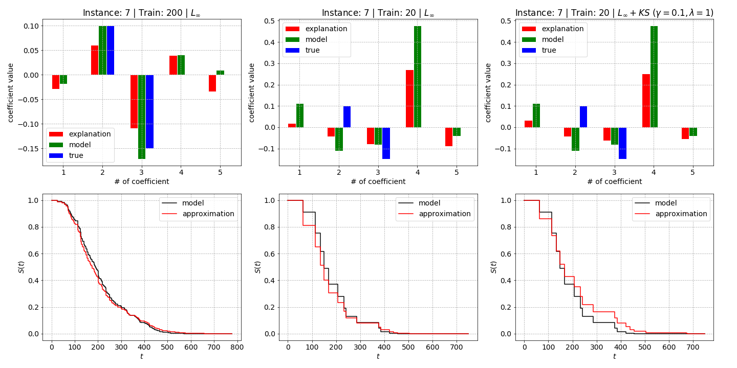
The corresponding results are illustrated in Figs. 3-5. In particular, Fig. 3 shows three considered cases of experiments (every column of pictures). The first row illustrates the coefficients of important features for the three conditions, where “model” or are coefficients of the Cox model which is used as the black-box model; “true” or are coefficients used for training data generation (see (61)); “explanation” or are explaining coefficients obtained by using the proposed algorithm. One can see from Fig. 3 that coefficients are close to and to at the first picture because the black-box Cox model is trained on the large dataset, and this trained model is of the high quality. A different relationship is observed in the second and the third pictures of the first row, which correspond to condition of small data. At the same time, it can be seen from these pictures that the explanation almost coincides with the coefficients of the black-box Cox model . This is due to the fact that we explain the model results, i.e., results obtained by the black-box Cox model, but not the training dataset. The second row of pictures in Fig. 3 illustrates how the SFs obtained by means of the black-box Cox model (“model”) and by means of the approximating Cox model (“approximation”) are close to each other. It can be seen from these pictures that the corresponding SFs under condition of large data are very close to each other. Moreover, we can clearly see that the lack of imprecision for small data provides better results than the use of KS bounds. Fig. 3 is an example of a “bad” case when the introduction of KS bounds leads to the worse approximation and explanation. A similar example is illustrated in Fig. 4. In contrast to the examples in Figs. 3 and 4, Fig. 5 illustrates a “good” case when the introduction of KS bounds leads to the better approximation and explanation.


9.1.3 The RSF
The second part of numerical experiments is performed with the RSF as a black-box model. We again study how the MRSE depends on the hyper-parameter of the regularization and the probability . The corresponding results are shown in Fig. 6. We can observe quite different results. It can be seen from Fig. 6 that the smallest value of the MRSE is achieved for very small values of . This implies that the introduction of KS bounds leads to the best results. The same can be seen from Table 2, where the RSE measures under different conditions of the experiment are shown for training examples. The measure is obtained under condition . It can be seen from Table 1 that, in contrast to the previous experiments (with the black-box Cox model), the studied part of experiments shows outperforming results with the KS bounds for most examples ( from ).

| datasets | |||
|---|---|---|---|
| large | small | ||
| examples | |||
| 0 | |||
| 1 | |||
| 2 | |||
| 3 | |||
| 4 | |||
| 5 | |||
| 6 | |||
| 7 | |||
| 8 | |||
| 9 | |||
The corresponding results are illustrated in Figs. 7-9. In particular, Fig. 7 shows three considered cases of experiments. Values of coefficients of important features are not depicted for the RSF because the RSF does not provide the important features like the Cox model. All figures illustrate pairs of SFs obtained by means of the RSF and by means of the approximating Cox model. Figs. 7 and 8 are examples of a “good” case when the introduction of KS bounds leads to the better approximation and explanation. In contrast to the examples in Figs. 7 and 8, Fig. 9 illustrates a “bad” case when the introduction of KS bounds leads to the worse approximation and explanation.


9.1.4 Contamination case
The next part of numerical experiments aims to study how the proposed explanation model deals with contaminated data, i.e., the objective is to get the black-box model explanation which is robust to contaminated data. In order to describe or generate so-called outliers in univariate statistical survival data, we assume that some subset of examples from all training examples is shifted, whereas other examples still come from some common target distribution. Two clusters of covariates are randomly generated such that points of every cluster are generated from the uniform distribution in the unit sphere. Centers of clusters are and , respectively. Parameters of the generated clusters are chosen such that the clusters do not intersect each other. The second cluster with the center is viewed as contaminated data. The number of points in every cluster is . They are depicted in Fig. 10 using the well-known t-SNE algorithm.
Times to event are generated by using (61) with parameters , , and , where and are coefficient of the Cox model for generating random points from clusters and , respectively. The parameters are taken in a way to get distinguished sets of SFs for both clusters as it is shown in Fig. 11, where two areas of SFs are depicted corresponding to different clusters.


Two cases are studied: the black-box model is trained on the large dataset ( examples) and on the small dataset ( examples). The model is tested on examples.
The basic (uncontaminated) large training set is formed from randomly selected examples of cluster . The basic (uncontaminated) small training set is formed from randomly selected examples of the same cluster. The contaminated dataset is formed as follows. We find the largest time to event from uncontaminated examples. The first quarter of the uncontaminated set consisting of and examples from the large and small datasets, respectively, is selected. These examples are replaced with examples from cluster 1 having times to event larger than . As a result, we have a mix of two clusters. For numerical experiments, we consider two methods: without KS bounds and with KS bounds. In sum, we get four cases for studying:
Case 1. The explanation model without KS bounds is trained on the uncontaminated dataset.
Case 2. The explanation model with KS bounds is trained on the uncontaminated dataset.
Case 3. The explanation model without KS bounds is trained on the contaminated dataset.
Case 4. The explanation model with KS bounds is trained on the contaminated dataset.
Measures are computed for Cases 1-4 denoted as , , , , respectively, by testing examples. The results of numerical experiments corresponding to all the considered cases for the black-box Cox model and the RSF are shown in Table 3 where the best performance on each dataset is shown in bold. It can be seen from Table 3 that three cases from four ones of the contaminated dataset show outperforming results by using KS bounds. Moreover, when the studied black-box model is the RSF, then the use of KS bounds in all cases leads to better results.
| dataset | uncontaminated | contaminated | |||
|---|---|---|---|---|---|
| without KS | with KS | without KS | with KS | ||
| model | |||||
| large | Cox | ||||
| large | RSF | ||||
| small | Cox | ||||
| small | RSF | ||||
In order to illustrate the difference between the results, we show the SFs in Figs. 12-15. Every figure consists of four pictures illustrating a pair of the black-box model SF and the approximating SF. Pictures in the first (the second) row show SFs of models trained on the uncontaminated (contaminated) dataset. Pictures in the first (the second) column illustrate SFs obtained without (with) using KS bounds. The same pictures can be found in Figs. 13-15. Results in Figs. 12-15 confirm conclusions which have been made by analyzing Table 3. In the case of uncontaminated datasets, the use of KS bounds gives comparable approximations except for the case of the RSF trained on the small dataset (see Fig. 15). At the same time, one can see quite different results when the black-box models are trained on the contaminated datasets where the use of KS bounds provides outperforming or comparable approximations. Moreover, the quality of approximation increases when the models are trained on the small dataset.


9.2 Numerical experiments with real data
We consider the following well-known real datasets to study SurvLIME-KS.
The Veterans’ Administration Lung Cancer Study (Veteran) Dataset [37] contains data on 137 males with advanced inoperable lung cancer. The subjects were randomly assigned to either a standard chemotherapy treatment or a test chemotherapy treatment. Several additional variables were also measured on the subjects. The number of features is 6, but it is extended till 9 due to categorical features.
The NCCTG Lung Cancer (LUNG) Dataset [44] records the survival of patients with advanced lung cancer, together with assessments of the patients performance status measured either by the physician and by the patients themselves. The data set contains 228 patients, including 63 patients that are right censored (patients that left the study before their death). The number of features is 8, but it is extended till 11 due to categorical features.
The above datasets can be downloaded via R package “survival”.
Approximation accuracy measures (, , ) are obtained for three cases: 1) approximating without KS bounds on the large dataset; 2) approximating without KS bounds on the small dataset; 3) approximating with KS bounds on the small dataset. The corresponding results for the black-box Cox model and the RSF trained on the Veteran dataset are shown in Table 4. It can be seen from Table 4 that the Cox model provides better results without KS bounds for the large dataset as well as the small dataset. The RSF shows quite different results. One can see that the introduction of KS bounds gives better result shown in bold ( from ). We again show in bold only results corresponding to the use of KS bounds.
| Cox model | RSF | |||||
|---|---|---|---|---|---|---|
| dataset | large | small | large | small | ||
| 0 | ||||||
| 1 | ||||||
| 2 | ||||||
| 3 | ||||||
| 4 | ||||||
| 5 | ||||||
| 6 | ||||||
| 7 | ||||||
| 8 | ||||||
| 9 | ||||||
Similar results for the LUNG dataset are given in Table 5. The use of KS bounds for this dataset shows even better results than for the Veteran dataset. One can see from Table 5 that outperforming results are available for the small dataset with using the Cox model.
| Cox model | RSF | |||||
|---|---|---|---|---|---|---|
| dataset | large | small | large | small | ||
| 0 | ||||||
| 1 | ||||||
| 2 | ||||||
| 3 | ||||||
| 4 | ||||||
| 5 | ||||||
| 6 | ||||||
| 7 | ||||||
| 8 | ||||||
| 9 | ||||||
Fig. 16 illustrates numerical results for the black-box Cox model trained on the Veteran dataset again under three conditions (approximating without KS bounds on the large dataset; approximating without KS bounds on the small dataset; approximating with KS bounds on the small dataset). The first row of pictures in Fig. 16 illustrates the coefficients of important features for the three conditions (see similar pictures in Figs. 3-5 for synthetic data). Two vectors of features are depicted in the form of diagrams: and . The second row of pictures in Fig. 16 illustrates how the SFs obtained by means of the black-box Cox model (“model”) and by means of the approximating Cox model (“approximation”) are close to each other. The same results for the RSF trained on the Veteran dataset are shown in Fig. 17.


10 Conclusion
A new robust explanation algorithm called SurvLIME-KS which can be regarded as a modification of the method SurvLIME has been presented in the paper. Its aim is to get robust explanation under condition of small training data and possible outliers. The basic idea behind the method is to approximate a set of CHFs, which are predicted by the black-box survival model and are restricted by KS bounds, by the CHF of the Cox proportional hazards model. The approximating Cox model allows us to get important features explaining the survival model. In contrast to SurvLIME, the proposed algorithm considers sets of CHFs produced by the KS bounds.
Various numerical experiments with synthetic and real data have illustrated the advantage of SurvLIME-KS in comparison with SurvLIME for certain conditions on the training data.
It should be noted that we have used KS bounds which are rather conservative bounds. However, there are other interesting bounds and imprecise statistical models which also could be studied and incorporated into SurvLIME to get robust algorithms, for example, the imprecise Dirichlet model [79], the imprecise pari-mutuel model, the linear-vacuous mixture or -contaminated model, the constant odds-ratio model [78]. These models may significantly improve the algorithm under some conditions. Their use is another direction for further research.
We have studied only the case when KS bounds are used for predicted CHFs which are produced by the black-box survival model. However, it is very interesting to consider the same bounds or other bounds for CHFs produced by the approximating Cox model. This case is more complicated, but it may enhance robust properties of the algorithm. This is also a direction for further research.
Acknowledgement
The reported study was funded by RFBR, project number 20-01-00154.
References
- [1] J. Abellan, R.M. Baker, F.P.A. Coolen, R.J. Crossman, and A.R. Masegosa. Classification with decision trees from a nonparametric predictive inference perspective. Computational Statistics and Data Analysis, 71:789–802, 2014.
- [2] J. Abellan, C.J. Mantas, and J.G. Castellano. A random forest approach using imprecise probabilities. Knowledge-Based Systems, 134:72–84, 2017.
- [3] J. Abellan, C.J. Mantas, J.G. Castellano, and S. Moral-Garcia. Increasing diversity in random forest learning algorithm via imprecise probabilities. Expert Systems With Applications, 97:228–243, 2018.
- [4] J. Abellan and S. Moral. Building classification trees using th building classification trees using the total uncertainty criterion. International Journal of Intelligent Systems, 18(12):1215–1225, 2003.
- [5] A. Adadi and M. Berrada. Peeking inside the black-box: A survey on explainable artificial intelligence (XAI). IEEE Access, 6:52138–52160, 2018.
- [6] I. Ahern, A. Noack, L. Guzman-Nateras, D. Dou, B. Li, and J. Huan. NormLime: A new feature importance metric for explaining deep neural networks. arXiv:1909.04200, Sep 2019.
- [7] A.B. Arrieta, N. Diaz-Rodriguez, J. Del Ser, A. Bennetot, S. Tabik, A. Barbado, S. Garcia, S. Gil-Lopez, D. Molina, R. Benjamins, R. Chatila, and F. Herrera. Explainable artificial intelligence (XAI): Concepts, taxonomies, opportunities and challenges toward responsible AI. arXiv:1910.10045, October 2019.
- [8] V. Arya, R.K.E. Bellamy, P.-Y. Chen, A. Dhurandhar, M. Hind, S.C. Hoffman, S. Houde, Q.V. Liao, R. Luss, A. Mojsilovic, S. Mourad, P. Pedemonte, R. Raghavendra, J. Richards, P. Sattigeri, K. Shanmugam, M. Singh, K.R. Varshney, D. Wei, and Y. Zhang. One explanation does not fit all: A toolkit and taxonomy of AI explainability techniques. arXiv:1909.03012, Sep 2019.
- [9] F. Barthe, O. Guedon, S. Mendelson, and A. Naor. A probabilistic approach to the geometry of the l-ball. The Annals of Probability, 33(2):480–513, 2005.
- [10] R. Bender, T. Augustin, and M. Blettner. Generating survival times to simulate cox proportional hazards models. Statistics in Medicine, 24(11):1713–1723, 2005.
- [11] M. Bickis. The imprecise logit-normal model and its application to estimating hazard functions. Journal of Statistical Theory and Practice, 3(1):183–195, 2009.
- [12] M. Bickis and U. Bickis. Predicting the next pandemic: An exercise in imprecise hazards. In 5th International Symposium on Imprecise Probability: Theories and Applications, pages 41–46, Prague, Czech Republic, 2007.
- [13] L. Breiman. Random forests. Machine learning, 45(1):5–32, 2001.
- [14] D.V. Carvalho, E.M. Pereira, and J.S. Cardoso. Machine learning interpretability: A survey on methods and metrics. Electronics, 8(832):1–34, 2019.
- [15] F.P.A. Coolen. An imprecise Dirichlet model for Bayesian analysis of failure data including right-censored observations. Reliability Engineering and System Safety, 56:61–68, 1997.
- [16] F.P.A. Coolen and K.J. Yan. Nonparametric predictive inference withright-censored data. Journal of Statistical Planning andInference, 126:25–54, 2004.
- [17] G. Corani and M. Zaffalon. Learning reliable classifiers from small or incomplete data sets: the naive credal classifier 2. Journal of Machine Learning Research, 9:581–621, 2008.
- [18] D.R. Cox. Regression models and life-tables. Journal of the Royal Statistical Society, Series B (Methodological), 34(2):187–220, 1972.
- [19] S. Destercke and V. Antoine. Combining imprecise probability masses with maximal coherent subsets: Application to ensemble classification. In Synergies of Soft Computing and Statistics for Intelligent Data Analysis, pages 27–35. Springer, Berlin, Heidelberg, 2013.
- [20] M. Du, N. Liu, and X. Hu. Techniques for interpretable machine learning. arXiv:1808.00033, May 2019.
- [21] D. Faraggi and R. Simon. A neural network model for survival data. Statistics in medicine, 14(1):73–82, 1995.
- [22] R. Fong and A. Vedaldi. Explanations for attributing deep neural network predictions. In Explainable AI, volume 11700 of LNCS, pages 149–167. Springer, Cham, 2019.
- [23] R.C. Fong and A. Vedaldi. Interpretable explanations of black boxes by meaningful perturbation. In Proceedings of the IEEE International Conference on Computer Vision, pages 3429–3437. IEEE, 2017.
- [24] D. Garreau and U. von Luxburg. Explaining the explainer: A first theoretical analysis of LIME. arXiv:2001.03447, January 2020.
- [25] Y. Goyal, Z. Wu, J. Ernst, D. Batra, D. Parikh, and S. Lee. Counterfactual visual explanations. arXiv:1904.07451, Apr 2019.
- [26] R. Guidotti, A. Monreale, S. Ruggieri, F. Turini, F. Giannotti, and D. Pedreschi. A survey of methods for explaining black box models. ACM computing surveys, 51(5):93, 2019.
- [27] C. Haarburger, P. Weitz, O. Rippel, and D. Merhof. Image-based survival analysis for lung cancer patients using CNNs. arXiv:1808.09679v1, Aug 2018.
- [28] R. Harman and V. Lacko. On decompositional algorithms for uniform sampling from n-spheres and n-balls. Journal of Multivariate Analysis, 101:2297–2304, 2010.
- [29] F. Harrell, R. Califf, D. Pryor, K. Lee, and R. Rosati. Evaluating the yield of medical tests. Journal of the American Medical Association, 247:2543–2546, 1982.
- [30] L.A. Hendricks, R. Hu, T. Darrell, and Z. Akata. Grounding visual explanations. In Proceedings of the European Conference on Computer Vision (ECCV), pages 264–279, 2018.
- [31] A. Holzinger, G. Langs, H. Denk, K. Zatloukal, and H. Muller. Causability and explainability of artificial intelligence in medicine. WIREs Data Mining and Knowledge Discovery, 9(4):e1312, 2019.
- [32] D. Hosmer, S. Lemeshow, and S. May. Applied Survival Analysis: Regression Modeling of Time to Event Data. John Wiley & Sons, New Jersey, 2008.
- [33] L. Hu, J. Chen, V.N. Nair, and A. Sudjianto. Locally interpretable models and effects based on supervised partitioning (LIME-SUP). arXiv:1806.00663, Jun 2018.
- [34] Q. Huang, M. Yamada, Y. Tian, D. Singh, D. Yin, and Y. Chang. GraphLIME: Local interpretable model explanations for graph neural networks. arXiv:2001.06216, January 2020.
- [35] N.A. Ibrahim, A. Kudus, I. Daud, and M.R. Abu Bakar. Decision tree for competing risks survival probability in breast cancer study. International Journal Of Biological and Medical Research, 3(1):25–29, 2008.
- [36] N.L. Johnson and F. Leone. Statistics and experimental design in engineering and the physical sciences, volume 1. Wiley, New York, 1964.
- [37] J. Kalbfleisch and R. Prentice. The Statistical Analysis of Failure Time Data. John Wiley and Sons, New York, 1980.
- [38] J.L. Katzman, U. Shaham, A. Cloninger, J. Bates, T. Jiang, and Y. Kluger. Deepsurv: Personalized treatment recommender system using a Cox proportional hazards deep neural network. BMC medical research methodology, 18(24):1–12, 2018.
- [39] F.M. Khan and V.B. Zubek. Support vector regression for censored data (SVRc): a novel tool for survival analysis. In 2008 Eighth IEEE International Conference on Data Mining, pages 863–868. IEEE, 2008.
- [40] J. Kim, I. Sohn, S.-H. Jung, S. Kim, and C. Park. Analysis of survival data with group lasso. Communications in Statistics - Simulation and Computation, 41(9):1593–1605, 2012.
- [41] M.S. Kovalev, L.V. Utkin, and E.M. Kasimov. SurvLIME: A method for explaining machine learning survival models. arXiv:2003.08371, March 2020.
- [42] C. Lee, W.R. Zame, J. Yoon, and M. van der Schaar. Deephit: A deep learning approach to survival analysis with competing risks. In 32nd Association for the Advancement of Artificial Intelligence ( AAAI) Conference, pages 1–8, 2018.
- [43] A. Van Looveren and J. Klaise. Interpretable counterfactual explanations guided by prototypes. arXiv:1907.02584, Jul 2019.
- [44] C.L. Loprinzi, J.A. Laurie, H.S. Wieand, J.E. Krook, P.J. Novotny, J.W. Kugler, J. Bartel, M. Law, M. Bateman, and N.E. Klatt. Prospective evaluation of prognostic variables from patient-completed questionnaires. north central cancer treatment group. Journal of Clinical Oncology, 3(12):601–607, 1994.
- [45] S.M. Lundberg and S.-I. Lee. A unified approach to interpreting model predictions. In Advances in Neural Information Processing Systems, pages 4765–4774, 2017.
- [46] F. Mangili, A. Benavoli, C.P. de Campos, and M. Zaffalon. Reliable survival analysis based on the Dirichlet process. Biometrical Journal, 57(6):1002–1019, 2015.
- [47] C.J. Mantas and J. Abellan. Analysis and extension of decision trees based on imprecise probabilities: Application on noisy data. Expert Systems with Applications, 41(5):2514–2525, 2014.
- [48] T. Marosevic. A choice of norm in discrete approximation. Mathematical Communications, 1(2):147–152, 1996.
- [49] P.-A. Matt. Uses and computation of imprecise probabilities from statistical data and expert arguments. International Journal of Approximate Reasoning, 81:63–86, 2017.
- [50] U.B. Mogensen, H. Ishwaran, and T.A. Gerds. Evaluating random forests for survival analysis using prediction error curves. Journal of Statistical Software, 50(11):1–23, 2012.
- [51] C. Molnar. Interpretable Machine Learning: A Guide for Making Black Box Models Explainable. Published online, https://christophm.github.io/interpretable-ml-book/, 2019.
- [52] S. Moral. Learning with imprecise probabilities as model selection and averaging. International Journal of Approximate Reasoning, 109:111–124, 2019.
- [53] S. Moral-Garcia, C.J. Mantas, J.G. Castellano, M.D. Benitez, and J. Abellan. Bagging of credal decision trees for imprecise classification. Expert Systems with Applications, 141(Article 112944):1–9, 2020.
- [54] W.J. Murdoch, C. Singh, K. Kumbier, R. Abbasi-Asl, and B. Yua. Interpretable machine learning: definitions, methods, and applications. arXiv:1901.04592, Jan 2019.
- [55] V. Petsiuk, A. Das, and K. Saenko. Rise: Randomized input sampling for explanation of black-box models. arXiv:1806.07421, June 2018.
- [56] J. Rabold, H. Deininger, M. Siebers, and U. Schmid. Enriching visual with verbal explanations for relational concepts: Combining LIME with Aleph. arXiv:1910.01837v1, October 2019.
- [57] Y. Ramon, D. Martens, F. Provost, and T. Evgeniou. Counterfactual explanation algorithms for behavioral and textual data. arXiv:1912.01819, December 2019.
- [58] R. Ranganath, A. Perotte, N. Elhadad, and D. Blei. Deep survival analysis. arXiv:1608.02158, September 2016.
- [59] M.T. Ribeiro, S. Singh, and C. Guestrin. “Why should I trust You?” Explaining the predictions of any classifier. arXiv:1602.04938v3, Aug 2016.
- [60] M.T. Ribeiro, S. Singh, and C. Guestrin. Anchors: High-precision model-agnostic explanations. In AAAI Conference on Artificial Intelligence, pages 1527–1535, 2018.
- [61] C.P. Robert. The Bayesian Choice. Springer, New York, 1994.
- [62] C. Rudin. Stop explaining black box machine learning models for high stakes decisions and use interpretable models instead. Nature Machine Intelligence, 1:206–215, 2019.
- [63] S.M. Shankaranarayana and D. Runje. ALIME: Autoencoder based approach for local interpretability. arXiv:1909.02437, Sep 2019.
- [64] K. Sim and R. Hartley. Removing outliers using the norm. In IEEE Computer Society Conference on Computer Vision and Pattern Recognition (CVPR’06), volume 1, pages 485–494, New York, NY, USA, 2006.
- [65] E. Strumbel and I. Kononenko. An efficient explanation of individual classifications using game theory. Journal of Machine Learning Research, 11:1–18, 2010.
- [66] R. Tibshirani. The lasso method for variable selection in the cox model. Statistics in medicine, 16(4):385–395, 1997.
- [67] L.V. Utkin. A framework for imprecise robust one-class classification models. International Journal of Machine Learning and Cybernetics, 5(3):379–393, 2014.
- [68] L.V. Utkin. An imprecise extension of svm-based machine learning models. Neurocomputing, 331:18–32, 2019.
- [69] L.V. Utkin. An imprecise deep forest for classification. Expert Systems with Applications, 141(112978):1–11, 2020.
- [70] L.V. Utkin and F.P.A. Coolen. On reliability growth models using Kolmogorov-Smirnov bounds. International Journal of Performability Engineering, 7(1):5–19, 2011.
- [71] L.V. Utkin and F.P.A. Coolen. Classification with support vector machines and Kolmogorov-Smirnov bounds. Journal of Statistical Theory and Practice, 8(2):297–318, 2014.
- [72] L.V. Utkin, M.S. Kovalev, and F. Coolen. Robust regression random forests by small and noisy training data. In Proceedings of XXII International Conference on Soft Computing and Measurements (SCM)), pages 134–137, St. Petersburg, Russia, 2019. IEEE.
- [73] L.V. Utkin, M.S. Kovalev, A.A. Meldo, and F.P.A. Coolen. Imprecise extensions of random forests and random survival forests. In Proceedings of Machine Learning Research, volume 103, pages 404–413, 2019.
- [74] L.V. Utkin and A. Wiencierz. Improving over-fitting in ensemble regression by imprecise probabilities. Information Sciences, 317:315–328, 2015.
- [75] J. van der Waa, M. Robeer, J. van Diggelen, M. Brinkhuis, and M. Neerincx. Contrastive explanations with local foil trees. arXiv:1806.07470, June 2018.
- [76] M.N. Vu, T.D. Nguyen, N. Phan, and M.T. Thai R. Gera. Evaluating explainers via perturbation. arXiv:1906.02032v1, Jun 2019.
- [77] S. Wachter, B. Mittelstadt, and C. Russell. Counterfactual explanations without opening the black box: Automated decisions and the GPDR. Harvard Journal of Law & Technology, 31:841–887, 2017.
- [78] P. Walley. Statistical Reasoning with Imprecise Probabilities. Chapman and Hall, London, 1991.
- [79] P. Walley. Inferences from multinomial data: Learning about a bag of marbles. Journal of the Royal Statistical Society, Series B, 58:3–57, 1996. with discussion.
- [80] H. Wang and L. Zhou. Random survival forest with space extensions for censored data. Artificial intelligence in medicine, 79:52–61, 2017.
- [81] P. Wang, Y. Li, and C.K. Reddy. Machine learning for survival analysis: A survey. arXiv:1708.04649, August 2017.
- [82] A. White and A.dA. Garcez. Measurable counterfactual local explanations for any classifier. arXiv:1908.03020v2, November 2019.
- [83] A. Widodo and B.-S. Yang. Machine health prognostics using survival probability and support vector machine. Expert Systems with Applications, 38(7):8430–8437, 2011.
- [84] D.M. Witten and R. Tibshirani. Survival analysis with high-dimensional covariates. Statistical Methods in Medical Research, 19(1):29–51, 2010.
- [85] M.N. Wright, T. Dankowski, and A. Ziegler. Unbiased split variable selection for random survival forests using maximally selected rank statistics. Statistics in Medicine, 36(8):1272–1284, 2017.
- [86] N. Xie, G. Ras, M. van Gerven, and D. Doran. Explainable deep learning: A field guide for the uninitiated. arXiv:2004.14545, April 2020.
- [87] H. Xu, C. Caramanis, and S. Mannor. Robustness and regularization of support vector machines. The Journal of Machine Learning Research, 10(7):1485–1510, 2009.
- [88] M.R. Zafar and N.M. Khan. DLIME: A deterministic local interpretable model-agnostic explanations approach for computer-aided diagnosis systems. arXiv:1906.10263, Jun 2019.
- [89] M. Zaffalon. Credible classification for environmental problems. Environmental Modelling and Software, 20(8):1003 – 1012, 2005.
- [90] H.H. Zhang and W. Lu. Adaptive Lasso for Cox’s proportional hazards model. Biometrika, 94(3):691–703, 2007.
- [91] L. Zhao and D. Feng. Dnnsurv: Deep neural networks for survival analysis using pseudo values. arXiv:1908.02337v2, March 2020.
- [92] X. Zhu, J. Yao, and J. Huang. Deep convolutional neural network for survival analysis with pathological images. In 2016 IEEE International Conference on Bioinformatics and Biomedicine (BIBM), pages 544–547. IEEE, 2016.