跳到论文正文
W Papers独立论文阅读器 arXiv:2005.02172 论文正文 计算阅读时间 · 0%
引用这篇论文根据当前论文元数据生成,正式投稿前建议核对。


License: arXiv.org perpetual non-exclusive license
arXiv:2005.02172v1 [hep-th] 02 May 2020

Algebra for Fractional Statistics - interpolating from fermions to bosons

Satish Ramakrishna Email: ramakrishna@physics.rutgers.edu Affiliation: Department of Physics & Astronomy, Rutgers, The State University of New Jersey, 136 Frelinghuysen Road Piscataway, NJ 08854-8019
August 11, 2026
Abstract

This article constructs the Hilbert space for the algebra α​β−ei​θ​β​α=1\alpha\beta-e^{i\theta}\beta\alpha=1 that provides a continuous interpolation between the Clifford and Heisenberg algebras. This particular form is inspired by the properties of anyons. We study the eigenvalues of a generalized number operator (𝒩=β​α{\cal N}=\beta\alpha) and construct the Hilbert space, classified by values of a complex coordinate (λ0\lambda_{0}): the eigenvalues lie on a circle. For θ\theta being an irrational multiple of 2​π2\pi, we get an infinite-dimensional representation, however for a rational multiple (MN\frac{M}{N}) of 2​π2\pi, it is finite-dimensional, parametrized by the complex coordinate λ0\lambda_{0}. The case for N=2;θ=πN=2\>;\>\theta=\pi is the usual Clifford algebra for fermions, while the case for N=∞;θ=0N=\infty\>;\>\theta=0 is the Heisenberg algebra of bosons, albeit with two copies for positive and negative eigenvalues. We find a smooth transition from the fermion to the boson situation as N→∞N\rightarrow\infty from N=2N=2. After constructing the Hilbert space from the algebra, the cases for N=2,3N=2,3 can be mapped to S​U​(2)SU(2). Then, we motivate the study of coherent states, rather generally. The coherent states are eigenstates of α\alpha, the annihilation operator and are labeled by complex numbers for non-zero λ0\lambda_{0}.

The notion of fractional or generalized statistics has been studied intensively from many different directions. There are three main approaches. The oldest is the study of q-commutators (or q-statistics), which studied deviations from the Pauli principle by studying small deviations from the basic anti-commutator for fermions. The second is the study of q-deformed oscillators, which studies the deformation of the harmonic oscillator algebra under a rather general scheme. This second approach is further differentiated into whether we consider the non-bosonic states to be only singly-occupied or not. We approach this topic from the point of view of interpolating between fermions and bosons, with an aim to encompass fractional statistics, with variable occupancy.

We start with the following bracket relation, which we refer to as a θ\theta-commutator

α​β−ei​θ​β​α≡(α,β)θ=1\displaystyle\alpha\beta-e^{i\theta}\beta\alpha\equiv\bigg(\alpha,\beta\bigg)_{\theta}=1 (1)

Formally, this is a special case of q-on (or q-deformed) algebra, for q=ei​θq=e^{i\theta}, while the right-hand-side is 1 instead of the usual qNq^{N} for a q-deformed algebra. This may be regarded as an interpolation between the commutator for bosons and the anti-commutator for fermions. By analogy with the algebra for bosons and fermions, the operator α\alpha may be taken as the annihilation operator for the algebra, while β\beta is the creation operator, though we could switch the identifications and derive an entirely similar algebra (see Appendix 1). We do not assume that α\alpha and β\beta are hermitian conjugates of each other.

This algebra is also inspired by the braiding requirements for anyonic variables, where we can braid variables “over” and “under” each other, with factors e±i​θe^{\pm i\theta}. We have chosen to work with the plus sign in the above; accordingly, we will use the notation z=ei​θz=e^{i\theta}. We have two classes of possibilities for θ\theta. θ\theta could be a rational multiple of 2​π2\pi, i.e., of the form θ=2​π​MN\theta=\frac{2\pi M}{N} where M,NM,N are co-prime non-zero natural numbers: in full generality, we could assume that M<NM<N. Alternatively, θ\theta could be an irrational multiple of 2​π2\pi. We will primarily study the rational multiple case, but make comments where necessary about the other (irrational multiple) case. Note that with M=1M=1 and N=2N=2, the expression above reduces to a fermionic anti-commutator while for N=∞N=\infty, to a bosonic commutator.

For general integral NN, we begin by thinking of α,β\alpha,\beta as ordinary matrices and construct the vector space they operate on. As we will discover, the results will indeed satisfy the axioms for a Hilbert space - the defining eigenvectors will constitute a complete vector space and we can define the usual inner product with positive norm.

We start by considering the operator 𝒩=β​α{\cal N}=\beta\alpha. The following bracket relations can be quickly verified

(α,𝒩)θ=α\displaystyle\bigg(\alpha,{\cal N}\bigg)_{\theta}=\alpha (2)
(𝒩,β)θ=β\displaystyle\bigg({\cal N},\beta\bigg)_{\theta}=\beta (3)

These relations imply

𝒩​α=α​𝒩−1z\displaystyle{\cal N}\alpha=\alpha\frac{{\cal N}-1}{z}
𝒩​β=β⁡(1+z​𝒩)\displaystyle{\cal N}\beta=\beta(1+z{\cal N}) (4)

Suppose ϕ→a\vec{\phi}_{a} were an eigenvector of the operator 𝒩\cal N, with eigenvalue sas_{a}. If we were to operate on ϕ→a\vec{\phi}_{a} with α\alpha, using the above relations, we would get an eigenvector of 𝒩\cal N with eigenvalue sa−1z\frac{s_{a}-1}{z}. We could label this state ϕ→a−1\vec{\phi}_{a-1}. Conversely, β\beta takes the eigenvector ϕ→a−1\vec{\phi}_{a-1} and produces an eigenvector of 𝒩\cal N, presumably ϕ→a\vec{\phi}_{a}, with eigenvalue sas_{a}. In this sense, we can think of α\alpha and β\beta as decrementing and incrementing operators.

In fact, the recursion relation for the eigenvalues of the operator 𝒩\cal N is

sa=1+z​sa−1\displaystyle s_{a}=1+zs_{a-1} (5)

Next, we reason in the following manner. We define the real and imaginary parts of 𝒩{\cal N}, i.e., 𝒩R,𝒩I{\cal N}_{R},{\cal N}_{I} and require that [𝒩R,𝒩I]=0[{\cal N}_{R},{\cal N}_{I}]=0. This immediately implies that [𝒩,𝒩†]=0[{\cal N},{\cal N}^{\dagger}]=0, which condition is the definition of a ”normal” matrix, viz. 𝒩{\cal N} is a normal matrix. If 𝒩{\cal N} is normal, then 𝒩,𝒩†{\cal N},{\cal N}^{\dagger} and the combinations 𝒩𝒩†{\cal N}{\cal N}^{\dagger} and 𝒩†​𝒩{\cal N}^{\dagger}{\cal N} all commute with each other, i.e., they share the same eigenvectors.

Since 𝒩†​𝒩{\cal N}^{\dagger}{\cal N} and 𝒩𝒩†{\cal N}{\cal N}^{\dagger} are both hermitian, their eigenvectors form an orthonormal, complete set. In this orthonormal basis, since α\alpha is a decrementing operator, while β\beta is an incrementing operator, we immediately deduce that α\alpha is an upper-diagonal matrix, while β\beta is a lower-diagonal matrix. Additionally, it is possible to arrange things so that α\alpha and β\beta are transposes of each other, though this is not the only possibility (see the text after Equation (9)).

One consequence of the above is that any operator in this space can be written as a polynomial with powers of α\alpha and β\beta. This is because any operator will take states in this complete, orthonormal basis to linear combinations of the basis vectors. Such a linear combination of states can be formed by repeatedly applying powers of α\alpha and β\beta to a starting state such as ϕ→a\vec{\phi}_{a}. In addition, only specific types of combinations of α\alpha and β\beta commute with 𝒩\cal N, as discussed in Appendix 4.

Suppose we start with an eigenvector with eigenvalue (for the operator 𝒩\cal N) of λ0\lambda_{0}, with θ=2​π​MN\theta=2\pi\frac{M}{N}. Applying β\beta successively to this eigenvector produces new eigenvectors with eigenvalues: 1+z​λ0, 1+z+z2​λ0, 1+z+z2+z3​λ0,…,, 1+z+z2+…+zN−2+zN−1​λ0, 1+z+z2+…+zN−1+zN​λ0,…1+z\lambda_{0},\>1+z+z^{2}\lambda_{0},\>1+z+z^{2}+z^{3}\lambda_{0},...,,\>1+z+z^{2}+...+z^{N-2}+z^{N-1}\lambda_{0},\>1+z+z^{2}+...+z^{N-1}+z^{N}\lambda_{0},.... With θ\theta of the form 2​π​MN2\pi\frac{M}{N}, then 1+z+z2+…+zN−1=01+z+z^{2}+...+z^{N-1}=0 and zN=1z^{N}=1, so that the sequence of eigenvalues repeats after N−1N-1 applications of α\alpha to the starting eigenvector with eigenvalue λ0\lambda_{0}. There are thus NN independent eigenvalues. Also, we note that 1+z​λ0=λ0−(1+z+…+zN−2)zN−11+z\lambda_{0}=\frac{\lambda_{0}-(1+z+...+z^{N-2})}{z^{N-1}} etc., so that the sequence of eigenvalues of β\beta are the same as the eigenvalues of α\alpha, except they are traversed in the opposite direction upon repeated application of β\beta. This is how we would expect decrementing and incrementing operators to work on the eigenvectors.

In addition, the actual eigenvalues for the case M=1M=1 as well as the case M>1M>1, with M,NM,N co-prime are the same, just arrived at in different order. Hence, we could, in all generality, assume M=1M=1 (the α\alpha and β\beta are the same matrices if M>1M>1, just with permuted rows).

If θ\theta were an irrational multiple of 2​π2\pi, the eigenvalues would never repeat upon repeated applications of α\alpha or β\beta, yet, since the relations λ0→λ1=(1+z​λ0)\lambda_{0}\rightarrow\lambda_{1}=(1+z\lambda_{0}) and λ1→λ0=λ1−1z\lambda_{1}\rightarrow\lambda_{0}=\frac{\lambda_{1}-1}{z}, the set of eigenvalues of α\alpha and β\beta are the same, though infinite in number. Summarizing, the matrix representation of α\alpha and β\beta are NN-dimensional for θ=2​π​MN\theta=2\pi\frac{M}{N} and infinite-dimensional for θ\theta an irrational multiple of 2​π2\pi.

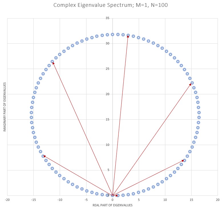
These eigenvalues sit on the same circle in the complex plane, for all θ\theta. For what follows, however, we specialize to the case where θ\theta is a rational multiple of 2​π2\pi and also set M=1M=1. Then we construct the matrix representations of α\alpha and β\beta in the eigen basis of 𝒩\cal N.

The sequence of eigenvalue points on the complex plane is λ0\lambda_{0}, followed by the successive eigenvalues 1+λ0​z,q+z+λ0​z2,q+z+z2+λ0​z3,…,1+z+z2+…+zN−2+λ0​zN−11+\lambda_{0}z,q+z+\lambda_{0}z^{2},q+z+z^{2}+\lambda_{0}z^{3},...,1+z+z^{2}+...+z^{N-2}+\lambda_{0}z^{N-1} (where, since M=1M=1, z=e2​π​iNz=e^{\frac{2\pi i}{N}}).

There are a few simple ways to show that these points lie on a circle. One method is as follows, a second is described in Appendix 2. The average of all the complex eigenvalues is 𝒵=11−z{\cal Z}=\frac{1}{1-z} (independent of λ0\lambda_{0}), which is the complex coordinate for the center. Then, the magnitude of the difference between each of the points in the above sequence and this central point is ℛ=|1+(z−1)×λ01−z|{\cal R}=|\frac{1+(z-1)\times\lambda_{0}}{1-z}|, i.e., each eigenvalue point is the same distance |1+(z−1)×λ01−z||\frac{1+(z-1)\times\lambda_{0}}{1-z}| from the center (see Appendix 2). This can then be identified as the radius of the circle.

Explicitly, the average of the points is 𝒪{\cal O}

=(λ0)+(1+z​λ0)+(1+z+z2​λ0)+(1+z+z2+z3​λ0)+…+(1+z+z2+…+zN−2+zN−1​λ0)N\displaystyle=\frac{(\lambda_{0})+(1+z\lambda_{0})+(1+z+z^{2}\lambda_{0})+(1+z+z^{2}+z^{3}\lambda_{0})+...+(1+z+z^{2}+...+z^{N-2}+z^{N-1}\lambda_{0})}{N}\>\>\>\>\>\>\>\>\>\>
=λ0​(1+z+z2+…+zN−1)+(N−1)​z0+(N−2)​z1+(N−3)​z2+…+(N−[N−1])​zN−2N\displaystyle=\frac{\lambda_{0}(1+z+z^{2}+...+z^{N-1})+(N-1)z^{0}+(N-2)z^{1}+(N-3)z^{2}+...+(N-[N-1])z^{N-2}}{N}\>\>\>\>\>\>\>\>\>\>\>\>\>\>\>\>\>\>\>
=0+(N−1)​z0+(N−2)​z1+(N−3)​z2+…+(N−[N−1])​zN−2N\displaystyle=\frac{0+(N-1)z^{0}+(N-2)z^{1}+(N-3)z^{2}+...+(N-[N-1])z^{N-2}}{N}\>\>\>\>\>\>\>\>\>\>\>\>\>\>\>\>\>\>\>\>\>\>\>\>\>\>\>\>\>\>\>\>\>\>\>\>\>\>
=11−z=i​e−i​θ22​sin⁡θ2=12+i2​tan⁡θ2\displaystyle=\frac{1}{1-z}=\frac{ie^{-i\frac{\theta}{2}}}{2\sin\frac{\theta}{2}}=\frac{1}{2}+\frac{i}{2\tan\frac{\theta}{2}}\>\>\>\>\>\>\>\>\>\>\>\>\>\>\>\>\>\>\>\>\>\>\>\>\>\>\>\>\>\>\>\>\>\>\>\>\>\>\>\>\>\>\>\>\>\>\>\>\>\>\>\>

i.e., the center of the eigenvalue circle is exactly at the same spot for all values of the starting eigenvalue λ0\lambda_{0}. The radius does depend on λ0\lambda_{0}, it is the magnitude of the difference between any eigenvalue and the complex coordinate of the center.

The angle between the lines connecting the center 11−z\frac{1}{1-z} and successive points 1+z+…+zp−2+λ0​zp−11+z+...+z^{p-2}+\lambda_{0}z^{p-1} and 1+z+z2+…+zp−1+λ0​zp1+z+z^{2}+...+z^{p-1}+\lambda_{0}z^{p} is easily computed by the ratio of the complex differences to the center - it is zz, i.e., the angle between the lines is θ\theta.

From the above, it is clear that we can label the representations (for a given NN) by either the complex number λ0\lambda_{0} (two real numbers) or the two real numbers representing the radius of the eigenvalue circle ℛ{\cal R} and the polar angle χ∈(0,2​πN)\chi\in(0,\frac{2\pi}{N}).

If λ0=0\lambda_{0}=0, then the first point in the above sequence is 00 and it is (one of the) lowest point(s) on the circle. When we consider non-zero λ0\lambda_{0}, that lowest point is mapped to a rotated point on a bigger circle (radius |1+(z−1)​λ0||1+(z-1)\lambda_{0}| with the same center. It is easily checked that the polar angle of the rotated point is bigger than that of the initial point by α=1i​log⁡1+(z−1)​λ0|1+(z−1)​λ0|\alpha=\frac{1}{i}\log\frac{1+(z-1)\lambda_{0}}{|1+(z-1)\lambda_{0}|}. This is easily proved to be true for every eigenvalue in the λ0=0\lambda_{0}=0 circle - it is rotated by the above angle when moved to the larger circle for λ0≠0\lambda_{0}\neq 0.

In addition, the magnitude of the separation distance between successive eigenvalues on the circle is |1+(z−1)​λ0||1+(z-1)\lambda_{0}|.

Figure 1: Eigenvalue Circle, M=1, N=100, λ0\lambda_{0}=0, as well as λ0=15+3​i\lambda_{0}=15+3i
Refer to caption
Refer to caption

Since α\alpha “decrements” states, it is an N×NN\times N matrix with upper diagonal non-zero terms only (as well as one in the bottom left corner to cycle through states again), in the basis where 𝒩=β​α{\cal N}=\beta\alpha is diagonal. Let’s state that β​α\beta\alpha is diagonal, with eigenvalues denoted by, say λi\lambda_{i}, i=0​…​(N−1)i=0...(N-1). Hence, purely by inspection and the expected upper-diagonal structure of α\alpha, as well as requiring that we “split” the eigenvalues to make β\beta and α\alpha transposes of each other, it must have λi+1\sqrt{\lambda_{i+1}} as elements. Hence the matrix α†​α\alpha^{\dagger}\alpha, by inspection, must have diagonal elements |λi||\lambda_{i}|, 0=1​…​(N−1)0=1...(N-1). Also by inspection, the matrices α​β\alpha\beta and α​α†\alpha\alpha^{\dagger} are diagonal; in fact, the elements of α​β\alpha\beta must be λi+1\lambda_{i+1}, i=0​…​(N−1)i=0...(N-1), where λN=λ0\lambda_{N}=\lambda_{0}. This additionally implies that the matrix α​α†\alpha\alpha^{\dagger} must have diagonal elements |λi+1||\lambda_{i+1}|, i=0​…​(N−1)i=0...(N-1).

Visually,

β​α=(λ𝟎   0   0   0   0...   000λ𝟏   0   0   0...   000   0λ𝟐   0   0...   000   0   0λ𝟑   0...   00...0   0   0   0   0...λ𝐍−𝟐00   0   0   0   0...   0λ𝐍−𝟏)\displaystyle\beta\alpha=\left(\begin{array}[]{cccccccc}{\bf\lambda_{0}}&\>\>\>0&\>\>\>0&\>\>\>0&\>\>\>0&...&\>\>\>0&0\\ 0&\>\>\>{\bf\lambda_{1}}&\>\>\>0&\>\>\>0&\>\>\>0&...&\>\>\>0&0\\ 0&\>\>\>0&\>\>\>{\bf\lambda_{2}}&\>\>\>0&\>\>\>0&...&\>\>\>0&0\\ 0&\>\>\>0&\>\>\>0&\>\>\>{\bf\lambda_{3}}&\>\>\>0&...&\>\>\>0&0\\ .\\ .\\ .\\ 0&\>\>\>0&\>\>\>0&\>\>\>0&\>\>\>0&...&\>\>\>{\bf\lambda_{N-2}}&0\\ 0&\>\>\>0&\>\>\>0&\>\>\>0&\>\>\>0&...&\>\>\>0&{\bf\lambda_{N-1}}\end{array}\right)
α​β=(λ𝟏   0   0   0   0...   000λ𝟐   0   0   0...   000   0λ𝟑   0   0...   000   0   0λ𝟒   0...   00...0   0   0   0   0...λ𝐍−𝟏00   0   0   0   0...   0λ𝟎)\displaystyle\alpha\beta=\left(\begin{array}[]{cccccccc}{\bf\lambda_{1}}&\>\>\>0&\>\>\>0&\>\>\>0&\>\>\>0&...&\>\>\>0&0\\ 0&\>\>\>{\bf\lambda_{2}}&\>\>\>0&\>\>\>0&\>\>\>0&...&\>\>\>0&0\\ 0&\>\>\>0&\>\>\>{\bf\lambda_{3}}&\>\>\>0&\>\>\>0&...&\>\>\>0&0\\ 0&\>\>\>0&\>\>\>0&\>\>\>{\bf\lambda_{4}}&\>\>\>0&...&\>\>\>0&0\\ .\\ .\\ .\\ 0&\>\>\>0&\>\>\>0&\>\>\>0&\>\>\>0&...&\>\>\>{\bf\lambda_{N-1}}&0\\ 0&\>\>\>0&\>\>\>0&\>\>\>0&\>\>\>0&...&\>\>\>0&{\bf\lambda_{0}}\end{array}\right)
α=(𝟎λ1   0   0   0...   000   0λ2   0   0...   000   0   0λ3   0...   000   0   0   0λ4...   00...0   0   0   0   0...   0λN−1λ0   0   0   0   0...   0𝟎)\displaystyle\alpha=\left(\begin{array}[]{cccccccc}{\bf 0}&\>\>\>\sqrt{\lambda_{1}}&\>\>\>0&\>\>\>0&\>\>\>0&...&\>\>\>0&0\\ 0&\>\>\>{\bf 0}&\>\>\>\sqrt{\lambda_{2}}&\>\>\>0&\>\>\>0&...&\>\>\>0&0\\ 0&\>\>\>0&\>\>\>{\bf 0}&\>\>\>\sqrt{\lambda_{3}}&\>\>\>0&...&\>\>\>0&0\\ 0&\>\>\>0&\>\>\>0&\>\>\>{\bf 0}&\>\>\>\sqrt{\lambda_{4}}&...&\>\>\>0&0\\ .\\ .\\ .\\ 0&\>\>\>0&\>\>\>0&\>\>\>0&\>\>\>0&...&\>\>\>{\bf 0}&\sqrt{\lambda_{N-1}}\\ \sqrt{\lambda_{0}}&\>\>\>0&\>\>\>0&\>\>\>0&\>\>\>0&...&\>\>\>0&{\bf 0}\end{array}\right)
β=αT=(𝟎   0   0   0   0...   0λ0λ1   0   0   0   0...   000λ2   0   0   0...   000   0λ3   0   0...   000   0   0λ4   0...   00...0   0   0   0   0...λN−1𝟎)\displaystyle\beta=\alpha^{T}=\left(\begin{array}[]{cccccccc}{\bf 0}&\>\>\>0&\>\>\>0&\>\>\>0&\>\>\>0&...&\>\>\>0&\sqrt{\lambda_{0}}\\ \sqrt{\lambda_{1}}&\>\>\>{\bf 0}&\>\>\>0&\>\>\>0&\>\>\>0&...&\>\>\>0&0\\ 0&\>\>\>\sqrt{\lambda_{2}}&\>\>\>{\bf 0}&\>\>\>0&\>\>\>0&...&\>\>\>0&0\\ 0&\>\>\>0&\>\>\>\sqrt{\lambda_{3}}&\>\>\>{\bf 0}&\>\>\>0&...&\>\>\>0&0\\ 0&\>\>\>0&\>\>\>0&\>\>\>\sqrt{\lambda_{4}}&\>\>\>{\bf 0}&...&\>\>\>0&0\\ .\\ .\\ .\\ 0&\>\>\>0&\>\>\>0&\>\>\>0&\>\>\>0&...&\sqrt{\lambda_{N-1}}&{\bf 0}\end{array}\right)
α∗=(𝟎λ1∗   0   0   0...   000   0λ2∗   0   0...   000   0   0λ3∗   0...   000   0   0   0λ4∗...   00...0   0   0   0   0...   0λN−1∗λ0∗   0   0   0   0...   0𝟎)\displaystyle\alpha^{*}=\left(\begin{array}[]{cccccccc}{\bf 0}&\>\>\>\sqrt{\lambda_{1}^{*}}&\>\>\>0&\>\>\>0&\>\>\>0&...&\>\>\>0&0\\ 0&\>\>\>{\bf 0}&\>\>\>\sqrt{\lambda_{2}^{*}}&\>\>\>0&\>\>\>0&...&\>\>\>0&0\\ 0&\>\>\>0&\>\>\>{\bf 0}&\>\>\>\sqrt{\lambda_{3}^{*}}&\>\>\>0&...&\>\>\>0&0\\ 0&\>\>\>0&\>\>\>0&\>\>\>{\bf 0}&\>\>\>\sqrt{\lambda_{4}^{*}}&...&\>\>\>0&0\\ .\\ .\\ .\\ 0&\>\>\>0&\>\>\>0&\>\>\>0&\>\>\>0&...&\>\>\>{\bf 0}&\sqrt{\lambda_{N-1}^{*}}\\ \sqrt{\lambda_{0}^{*}}&\>\>\>0&\>\>\>0&\>\>\>0&\>\>\>0&...&\>\>\>0&{\bf 0}\end{array}\right)
β∗=α†=(𝟎   0   0   0   0...   0λ0∗λ1∗   0   0   0   0...   000λ2∗   0   0   0...   000   0λ3∗   0   0...   000   0   0λ4∗   0...   00...0   0   0   0   0...λN−1∗𝟎)\displaystyle\beta^{*}=\alpha^{\dagger}=\left(\begin{array}[]{cccccccc}{\bf 0}&\>\>\>0&\>\>\>0&\>\>\>0&\>\>\>0&...&\>\>\>0&\sqrt{\lambda_{0}^{*}}\\ \sqrt{\lambda_{1}^{*}}&\>\>\>{\bf 0}&\>\>\>0&\>\>\>0&\>\>\>0&...&\>\>\>0&0\\ 0&\>\>\>\sqrt{\lambda_{2}^{*}}&\>\>\>{\bf 0}&\>\>\>0&\>\>\>0&...&\>\>\>0&0\\ 0&\>\>\>0&\>\>\>\sqrt{\lambda_{3}^{*}}&\>\>\>{\bf 0}&\>\>\>0&...&\>\>\>0&0\\ 0&\>\>\>0&\>\>\>0&\>\>\>\sqrt{\lambda_{4}^{*}}&\>\>\>{\bf 0}&...&\>\>\>0&0\\ .\\ .\\ .\\ 0&\>\>\>0&\>\>\>0&\>\>\>0&\>\>\>0&...&\sqrt{\lambda_{N-1}^{*}}&{\bf 0}\end{array}\right)
α†​α=(|λ𝟎|   0   0   0   0...   000|λ𝟏|   0   0   0...   000   0|λ𝟐|   0   0...   000   0   0|λ𝟑|   0...   00...0   0   0   0   0...|λ𝐍−𝟐|00   0   0   0   0...   0|λ𝐍−𝟏|)\displaystyle\alpha^{\dagger}\alpha=\left(\begin{array}[]{cccccccc}{\bf|\lambda_{0}|}&\>\>\>0&\>\>\>0&\>\>\>0&\>\>\>0&...&\>\>\>0&0\\ 0&\>\>\>{\bf|\lambda_{1}|}&\>\>\>0&\>\>\>0&\>\>\>0&...&\>\>\>0&0\\ 0&\>\>\>0&\>\>\>{\bf|\lambda_{2}|}&\>\>\>0&\>\>\>0&...&\>\>\>0&0\\ 0&\>\>\>0&\>\>\>0&\>\>\>{\bf|\lambda_{3}|}&\>\>\>0&...&\>\>\>0&0\\ .\\ .\\ .\\ 0&\>\>\>0&\>\>\>0&\>\>\>0&\>\>\>0&...&\>\>\>{\bf|\lambda_{N-2}|}&0\\ 0&\>\>\>0&\>\>\>0&\>\>\>0&\>\>\>0&...&\>\>\>0&{\bf|\lambda_{N-1}|}\end{array}\right)
α​α†=(|λ𝟏|   0   0   0   0...   000|λ𝟐|   0   0   0...   000   0|λ𝟑|   0   0...   000   0   0|λ𝟒|   0...   00...0   0   0   0   0...|λ𝐍−𝟏|00   0   0   0   0...   0|λ𝟎|)\displaystyle\alpha\alpha^{\dagger}=\left(\begin{array}[]{cccccccc}{\bf|\lambda_{1}|}&\>\>\>0&\>\>\>0&\>\>\>0&\>\>\>0&...&\>\>\>0&0\\ 0&\>\>\>{\bf|\lambda_{2}|}&\>\>\>0&\>\>\>0&\>\>\>0&...&\>\>\>0&0\\ 0&\>\>\>0&\>\>\>{\bf|\lambda_{3}|}&\>\>\>0&\>\>\>0&...&\>\>\>0&0\\ 0&\>\>\>0&\>\>\>0&\>\>\>{\bf|\lambda_{4}|}&\>\>\>0&...&\>\>\>0&0\\ .\\ .\\ .\\ 0&\>\>\>0&\>\>\>0&\>\>\>0&\>\>\>0&...&\>\>\>{\bf|\lambda_{N-1}|}&0\\ 0&\>\>\>0&\>\>\>0&\>\>\>0&\>\>\>0&...&\>\>\>0&{\bf|\lambda_{0}|}\end{array}\right)

We can now write down regular and θ\theta commutators for α\alpha and α†\alpha^{\dagger} too, as

α​β−β​α=(λ𝟏−λ𝟎   0   0   0   0...   000λ𝟐−λ𝟏   0   0   0...   000   0λ𝟑−λ𝟐   0   0...   000   0   0λ𝟒−λ𝟑   0...   00...0   0   0   0   0...λ𝐍−𝟏−λ𝐍−𝟐00   0   0   0   0...   0λ𝟎−λ𝐍−𝟏)\displaystyle\alpha\beta-\beta\alpha=\left(\begin{array}[]{cccccccc}{\bf\lambda_{1}-\lambda_{0}}&\>\>\>0&\>\>\>0&\>\>\>0&\>\>\>0&...&\>\>\>0&0\\ 0&\>\>\>{\bf\lambda_{2}-\lambda_{1}}&\>\>\>0&\>\>\>0&\>\>\>0&...&\>\>\>0&0\\ 0&\>\>\>0&\>\>\>{\bf\lambda_{3}-\lambda_{2}}&\>\>\>0&\>\>\>0&...&\>\>\>0&0\\ 0&\>\>\>0&\>\>\>0&\>\>\>{\bf\lambda_{4}-\lambda_{3}}&\>\>\>0&...&\>\>\>0&0\\ .\\ .\\ .\\ 0&\>\>\>0&\>\>\>0&\>\>\>0&\>\>\>0&...&\>\>\>{\bf\lambda_{N-1}-\lambda_{N-2}}&0\\ 0&\>\>\>0&\>\>\>0&\>\>\>0&\>\>\>0&...&\>\>\>0&{\bf\lambda_{0}-\lambda_{N-1}}\end{array}\right)

and

α​α†−α†​α\displaystyle\alpha\alpha^{\dagger}-\alpha^{\dagger}\alpha\>\>\>\>\>\>\>\>\>\>\>\>\>\>\>\>\>\>\>\>\>\>\>\>\>\>\>\>\>\>\>\>\>\>\>\>\>\>\>\>\>\>\>\>\>\>\>\>\>\>\>\>\>\>\>\>\>\>\>\>\>\>\>\>\>\>\>\>\>\>\>\>\>\>\>\>\>\>\>\>
=(|λ𝟏|−|λ𝟎|   0   0   0   0...   000|λ𝟐|−|λ𝟏|   0   0   0...   000   0|λ𝟑|−|λ𝟐|   0   0...   000   0   0|λ𝟒|−|λ𝟑|   0...   00...0   0   0   0   0...|λ𝐍−𝟏|−|λ𝐍−𝟐|00   0   0   0   0...   0|λ𝟎|−|λ𝐍−𝟏|)\displaystyle=\left(\begin{array}[]{cccccccc}{\bf|\lambda_{1}|-|\lambda_{0}|}&\>\>\>0&\>\>\>0&\>\>\>0&\>\>\>0&...&\>\>\>0&0\\ 0&\>\>\>{\bf|\lambda_{2}|-|\lambda_{1}|}&\>\>\>0&\>\>\>0&\>\>\>0&...&\>\>\>0&0\\ 0&\>\>\>0&\>\>\>{\bf|\lambda_{3}|-|\lambda_{2}|}&\>\>\>0&\>\>\>0&...&\>\>\>0&0\\ 0&\>\>\>0&\>\>\>0&\>\>\>{\bf|\lambda_{4}|-|\lambda_{3}|}&\>\>\>0&...&\>\>\>0&0\\ .\\ .\\ .\\ 0&\>\>\>0&\>\>\>0&\>\>\>0&\>\>\>0&...&\>\>\>{\bf|\lambda_{N-1}|-|\lambda_{N-2}|}&0\\ 0&\>\>\>0&\>\>\>0&\>\>\>0&\>\>\>0&...&\>\>\>0&{\bf|\lambda_{0}|-|\lambda_{N-1}|}\end{array}\right)

as well as

α​α†−𝒞​α†​α=1→\displaystyle\alpha\alpha^{\dagger}-{\cal C}\alpha^{\dagger}\alpha=1\rightarrow\>\>\>\>\>\>\>\>\>\>\>\>\>\>\>\>\>\>\>\>\>\>\>\>\>\>\>\>\>\>\>\>\>\>\>\>\>\>\>\>\>\>\>\>\>\>\>\>\>\>\>\>\>\>\>\>\>\>\>\>\>\>\>\>\>\>\>\>\>\>\>\>\>\>\>\>\>\>\>\>
𝒞=(|λ𝟏|−𝟏|λ𝟎|   0   0   0   0...   000|λ𝟐|−𝟏|λ​𝟏|   0   0   0...   000   0|λ𝟑|−𝟏|λ𝟐|   0   0...   000   0   0|λ𝟒|−𝟏|λ𝟑|   0...   00...0   0   0   0   0...|λ𝐍−𝟏|−𝟏|λ𝐍−𝟐|00   0   0   0   0...   0|λ𝟎|−𝟏|λ𝐍−𝟏|)\displaystyle{\cal C}=\left(\begin{array}[]{cccccccc}{\bf\frac{|\lambda_{1}|-1}{|\lambda_{0}|}}&\>\>\>0&\>\>\>0&\>\>\>0&\>\>\>0&...&\>\>\>0&0\\ 0&\>\>\>{\bf\frac{|\lambda_{2}|-1}{|\lambda 1|}}&\>\>\>0&\>\>\>0&\>\>\>0&...&\>\>\>0&0\\ 0&\>\>\>0&\>\>\>{\bf\frac{|\lambda_{3}|-1}{|\lambda_{2}|}}&\>\>\>0&\>\>\>0&...&\>\>\>0&0\\ 0&\>\>\>0&\>\>\>0&\>\>\>{\bf\frac{|\lambda_{4}|-1}{|\lambda_{3}|}}&\>\>\>0&...&\>\>\>0&0\\ .\\ .\\ .\\ 0&\>\>\>0&\>\>\>0&\>\>\>0&\>\>\>0&...&\>\>\>{\bf\frac{|\lambda_{N-1}|-1}{|\lambda_{N-2}|}}&0\\ 0&\>\>\>0&\>\>\>0&\>\>\>0&\>\>\>0&...&\>\>\>0&{\bf\frac{|\lambda_{0}|-1}{|\lambda_{N-1}|}}\end{array}\right)

Summarizing the results,

  1. 1.

    The eigenvalues of β​α\beta\alpha are λi\lambda_{i}

  2. 2.

    The eigenvalues of α†​α\alpha^{\dagger}\alpha are |λi||\lambda_{i}|.

  3. 3.

    𝒩†=α†​β†=α†​α∗=(αT​α)∗{\cal N}^{\dagger}=\alpha^{\dagger}\beta^{\dagger}=\alpha^{\dagger}\alpha^{*}=(\alpha_{T}\alpha)^{*}, i.e., the operator α†​β†\alpha^{\dagger}\beta^{\dagger} is diagonal in the same basis and has eigenvalues λi∗\lambda_{i}^{*}.

  4. 4.

    The eigenbasis of β​α\beta\alpha is also the eigenbasis for α†​α\alpha^{\dagger}\alpha, hence the eigenvectors can be constructed to be orthonormal, as will be shown below. In addition, the eigenbasis forms a Hilbert space, since the norms of the eigenvectors are positive-definite.

  5. 5.

    The operators 𝒩=β​α\cal N=\beta\alpha, 𝒩R=𝒩+𝒩†2=β​α+α†​β†2{\cal N}_{R}=\frac{{\cal N}+{\cal N}^{\dagger}}{2}=\frac{\beta\alpha+\alpha^{\dagger}\beta^{\dagger}}{2} and 𝒩I=𝒩−𝒩†2​i=β​α−α†​β†2​i{\cal N}_{I}=\frac{{\cal N}-{\cal N}^{\dagger}}{2i}=\frac{\beta\alpha-\alpha^{\dagger}\beta^{\dagger}}{2i} commute with each other and the eigenvalues of each are distinct. Hence, we can label the eigenvectors interchangeably by the eigenvalues of 𝒩{\cal N}, 𝒩R{\cal N}_{R} or 𝒩I{\cal N}_{I}.

  6. 6.

    In particular, since 𝒩R{\cal N}_{R} and 𝒩I{\cal N}_{I} are hermitian, the eigenvectors can be constructed to be orthonormal. In fact, noting the fact that the eigenvectors of a Hermitian matrix have positive norm, the space of eigenvectors satisfy all the axioms for a Hilbert space.

The above visual argument can be made precise. We start with an eigenvector of 𝒩\cal N, which is also an eigenstate of 𝒩R{\cal N}_{R} and 𝒩I{\cal N}_{I}), eigenvalue λ0\lambda_{0} under 𝒩\cal N (eigenvalues λ0+λ0∗2\frac{\lambda_{0}+\lambda_{0}^{*}}{2}, λ0−λ0∗2​i\frac{\lambda_{0}-\lambda_{0}^{*}}{2i} under 𝒩R{\cal N}_{R}, 𝒩I{\cal N}_{I} respectively). Then, we derive all the successive eigenvectors and their eigenvalues. As proved in Appendix 3, the eigenvectors of 𝒩R{\cal N}_{R}, 𝒩I{\cal N}_{I} and 𝒩{\cal N} are all the same and can be labeled simultaneously by the eigenvalues of the three operators, as 12​(λi+λi∗)\frac{1}{2}(\lambda_{i}+\lambda^{*}_{i}), 12​i​(λi−λi∗)\frac{1}{2i}(\lambda_{i}-\lambda^{*}_{i}) and λi\lambda_{i}. The eigenvalues we get by repeated applications of α\alpha are,

  1. 1.

    for 𝒩{\cal N}: λ0\lambda_{0}, λ0−1z\frac{\lambda_{0}-1}{z}, λ0−(1+z)z2\frac{\lambda_{0}-(1+z)}{z^{2}}, λ0−(1+z+z2)z3\frac{\lambda_{0}-(1+z+z^{2})}{z^{3}}, … λ0−(1+z+z2+…+zN−2)zN−1\frac{\lambda_{0}-(1+z+z^{2}+...+z^{N-2})}{z^{N-1}}, λ0−(1+z+z2+…+zN−1)zN,…\frac{\lambda_{0}-(1+z+z^{2}+...+z^{N-1})}{z^{N}},...\>\>.

  2. 2.

    for 𝒩R{\cal N}_{R}: Re λ0\lambda_{0}, Re λ0−1z\frac{\lambda_{0}-1}{z}, Re λ0−(1+z)z2\frac{\lambda_{0}-(1+z)}{z^{2}}, Re λ0−(1+z+z2)z3\frac{\lambda_{0}-(1+z+z^{2})}{z^{3}}, … Re λ0−(1+z+z2+…+zN−2)zN−1\frac{\lambda_{0}-(1+z+z^{2}+...+z^{N-2})}{z^{N-1}}, Re λ0−(1+z+z2+…+zN−1)zN,…\frac{\lambda_{0}-(1+z+z^{2}+...+z^{N-1})}{z^{N}},...\>\>.

  3. 3.

    for 𝒩I{\cal N}_{I}: Im λ0\lambda_{0}, Im λ0−1z\frac{\lambda_{0}-1}{z}, Im λ0−(1+z)z2\frac{\lambda_{0}-(1+z)}{z^{2}}, Im λ0−(1+z+z2)z3\frac{\lambda_{0}-(1+z+z^{2})}{z^{3}}, … Im λ0−(1+z+z2+…+zN−2)zN−1\frac{\lambda_{0}-(1+z+z^{2}+...+z^{N-2})}{z^{N-1}}, Im λ0−(1+z+z2+…+zN−1)zN,…\frac{\lambda_{0}-(1+z+z^{2}+...+z^{N-1})}{z^{N}},...\>\>.

Studying the above, since we already know that there are NN independent eigenvectors, the NN distinct eigenvalues of 𝒩\cal N are most appropriate to label the eigenvectors. The other commuting operators, viz 𝒩R{\cal N}_{R} and 𝒩I{\cal N}_{I} have degenerate eigenvalues, as is evident from an inspection of Fig. 2.

Hence, we define the normalized eigenstates of 𝒩=β​α{\cal N}=\beta\alpha as |λ0⟩,|λ1⟩,|λ2⟩,…,|λN−1⟩\ket{\lambda_0},\ket{\lambda_1},\ket{\lambda_2},...,\ket{\lambda_{N-1}}, where λ1=(1+zλ0),λ2=(1+z+z2λ0),…,λN−1=1+z+z2+…+zN−2+zN−1λ0\lambda_{1}=(1+z\lambda_{0}),\lambda_{2}=(1+z+z^{2}\lambda_{0}),...,\lambda_{N-1}=1+z+z^{2}+...+z^{N-2}+z^{N-1}\lambda_{0} and equivalently λ0=λ1−1z,λ1=λ2−1z,…,λN−1=λ0−1z\lambda_{0}=\frac{\lambda_{1}-1}{z},\lambda_{1}=\frac{\lambda_{2}-1}{z},...,\lambda_{N-1}=\frac{\lambda_{0}-1}{z}. Then, we construct the components of α\alpha and β\beta. We begin with the relationships (the CC’s and DD’s are normalization constants).

α​|λ0⟩=C0​|λN−1≡λ0−1z⟩\displaystyle\alpha\ket{\lambda_0}=C_{0}\ket{\lambda_{N-1} \equiv\frac{\lambda_0-1}{z}}
α​|λN−1⟩=CN−1​|sN−2=λ0−(1+z)z2≡λ0z2−1z−1z2⟩\displaystyle\alpha\ket{\lambda_{N-1}}=C_{N-1}\ket{s_{N-2}=\frac{\lambda_0 - (1+z)}{z^2} \equiv\frac{\lambda_0}{z^2}-\frac{1}{z}-\frac{1}{z^2}}
.
.
.
α​|λ0⟩=C0​|λN−1⟩\displaystyle\alpha\ket{\lambda_0}=C_{0}\ket{\lambda_{N-1}}
α​|λ1⟩=C1​|λ0⟩\displaystyle\alpha\ket{\lambda_1}=C_{1}\ket{\lambda_0}
α​|λ2⟩=C2​|λ1⟩\displaystyle\alpha\ket{\lambda_2}=C_{2}\ket{\lambda_1}
\displaystyle...
β​|λ0⟩=D0​|λ1≡(1+z​λ0)⟩\displaystyle\beta\ket{\lambda_0}=D_{0}\ket{\lambda_1 \equiv(1+z \lambda_0)}
β​|λ1⟩=D1​|λ2≡(1+z+z2​λ0)⟩\displaystyle\beta\ket{\lambda_1}=D_{1}\ket{\lambda_2 \equiv(1+z+z^2 \lambda_0)}
.
.
.
β​|λN−1⟩=DN−1​|λ0⟩\displaystyle\beta\ket{\lambda_{N-1}}=D_{N-1}\ket{\lambda_0} (116)

For consistency with the results of applying the number operator 𝒩=β​α{\cal N}=\beta\alpha to these states, given that λ0,λ1,…,λN−1\lambda_{0},\lambda_{1},...,\lambda_{N-1} are the eigenvalues of the number operator, we get the following conditions,

C0×DN−1=λ0\displaystyle C_{0}\times D_{N-1}=\lambda_{0}
C1×D0=λ1\displaystyle C_{1}\times D_{0}=\lambda_{1}
C2×D1=λ2\displaystyle C_{2}\times D_{1}=\lambda_{2}
.
.
.
CN−1×DN−2=λN−1\displaystyle C_{N-1}\times D_{N-2}=\lambda_{N-1} (117)

A natural choice (only one of several choices, though, as explained after Equation (9)) for the coefficients is

C0=DN−1=λ0\displaystyle C_{0}=D_{N-1}=\sqrt{\lambda_{0}}
C1=D0=λ1\displaystyle C_{1}=D_{0}=\sqrt{\lambda_{1}}
\displaystyle...
CN−1=DN−2=λN−1\displaystyle C_{N-1}=D_{N-2}=\sqrt{\lambda_{N-1}} (118)

This implies the matrix representations for the operators are

α=(𝟎C1   0   0   0...   000   0C2   0   0...   000   0   0C3   0...   000   0   0   0C4...   00...0   0   0   0   0...   0CN−1C0   0   0   0   0...   0𝟎)​β=(𝟎   0   0   0   0...   0DN−1D0   0   0   0   0...   000D1   0   0   0...   000   0D2   0   0...   000   0   0D3   0...   00...0   0   0   0   0...DN−2𝟎)\displaystyle\alpha=\left(\begin{array}[]{cccccccc}{\bf 0}&\>\>\>C_{1}&\>\>\>0&\>\>\>0&\>\>\>0&...&\>\>\>0&0\\ 0&\>\>\>{\bf 0}&\>\>\>C_{2}&\>\>\>0&\>\>\>0&...&\>\>\>0&0\\ 0&\>\>\>0&\>\>\>{\bf 0}&\>\>\>C_{3}&\>\>\>0&...&\>\>\>0&0\\ 0&\>\>\>0&\>\>\>0&\>\>\>{\bf 0}&\>\>\>C_{4}&...&\>\>\>0&0\\ .\\ .\\ .\\ 0&\>\>\>0&\>\>\>0&\>\>\>0&\>\>\>0&...&\>\>\>{\bf 0}&C_{N-1}\\ C_{0}&\>\>\>0&\>\>\>0&\>\>\>0&\>\>\>0&...&\>\>\>0&{\bf 0}\end{array}\right)\>\>\beta=\left(\begin{array}[]{cccccccc}{\bf 0}&\>\>\>0&\>\>\>0&\>\>\>0&\>\>\>0&...&\>\>\>0&D_{N-1}\\ D_{0}&\>\>\>{\bf 0}&\>\>\>0&\>\>\>0&\>\>\>0&...&\>\>\>0&0\\ 0&\>\>\>D_{1}&\>\>\>{\bf 0}&\>\>\>0&\>\>\>0&...&\>\>\>0&0\\ 0&\>\>\>0&\>\>\>D_{2}&\>\>\>{\bf 0}&\>\>\>0&...&\>\>\>0&0\\ 0&\>\>\>0&\>\>\>0&\>\>\>D_{3}&\>\>\>{\bf 0}&...&\>\>\>0&0\\ .\\ .\\ .\\ 0&\>\>\>0&\>\>\>0&\>\>\>0&\>\>\>0&...&D_{N-2}&{\bf 0}\end{array}\right)

These matrices are transposes (β=αT\beta=\alpha^{T}) of each other, based on the choice made in Equation (8) and the discussions after Equation (9).

Additionally, we find

βN=αN=C0×C1×…×CN−1=D0×D1×…×DN−1\displaystyle\beta^{N}=\alpha^{N}=C_{0}\times C_{1}\times...\times C_{N-1}=D_{0}\times D_{1}\times...\times D_{N-1}
=λ0×λ1×λ2×λ3​…×λN−1\displaystyle=\sqrt{\lambda_{0}\times\lambda_{1}\times\lambda_{2}\times\lambda_{3}...\times\lambda_{N-1}} (138)

For the special case λ0=0\lambda_{0}=0, this is 00.

It is not necessary for us to choose the conditions as in Equation (8), i.e., that β=αT\beta=\alpha^{T}. Suppose we chose to not pick this choice. In the basis where 𝒩{\cal N} is diagonal, however, we note a symmetry (based on a diagonal matrix 𝐐\bf Q)

α→α​𝐐\displaystyle\alpha\rightarrow\alpha{\bf Q}
β→𝐐−1​β\displaystyle\beta\rightarrow{\bf Q}^{-1}\beta
α​β−z​β​α→α​𝐐𝐐−1​β−z​𝐐−1​β​α​𝐐=1\displaystyle\alpha\beta-z\beta\alpha\rightarrow\alpha{\bf Q}{\bf Q}^{-1}\beta-z{\bf Q}^{-1}\beta\alpha{\bf Q}=1 (139)

such that the modified α\alpha and β\beta are transposes of each other. The eigenvalues of β​α\beta\alpha are, however, unaffected. The eigenvalues still sit on the same circle on the complex plane. Some further generalizations of the concepts discussed above can yield interesting deviations from a circle SatishUnpub.

Though the α\alpha and β=αT\beta=\alpha^{T} are λ0\lambda_{0}-dependent, the original θ\theta-commutator (Equation (1)) is independent of λ0\lambda_{0}, i.e., α​β−z​β​α=1\alpha\beta-z\beta\alpha=1. However, the usual commutator does dependent on λ0\lambda_{0}, through the eigenvalues of β​α\beta\alpha. In fact,

α​β−β​α=α​αT−αT​α=(1+(z−1)​β​α)\displaystyle\alpha\beta-\beta\alpha=\alpha\alpha^{T}-\alpha^{T}\alpha=\bigg(1+(z-1)\beta\alpha\bigg) (140)

The diagonal elements qmq_{m} of the commutator matrix in the usual eigenbasis are qm=1+(z−1)​smq_{m}=1+(z-1)s_{m}. This can be simply re-written as (for m>0\>m>0)

qm=1+(z−1)​sm=1+(z−1)​(1+z+z2+…+zm−1+zm​λ0)\displaystyle q_{m}=1+(z-1)s_{m}=1+(z-1)\bigg(1+z+z^{2}+...+z^{m-1}+z^{m}\lambda_{0}\bigg)
=zm−1​(1+(z−1)​λ0)\displaystyle=z^{m-1}\bigg(1+(z-1)\lambda_{0}\bigg)

Hence, we can write the full matrix form as below

α​β−β​α=α​αT−αT​α=(1+(z−1)​λ0)×(𝟏   0   0   0   0...00𝐳   0   0   0...   000   0𝐳𝟐   0   0...   000   0   0𝐳𝟑   0...   000   0   0   0𝐳𝟒...   00...0   0   0   0   0...𝐳𝐍−𝟐   00   0   0   0   0...   0𝐳𝐍−𝟏)\displaystyle\alpha\beta-\beta\alpha=\alpha\alpha^{T}-\alpha^{T}\alpha=(1+(z-1)\lambda_{0})\times\left(\begin{array}[]{cccccccc}{\bf 1}&\>\>\>0&\>\>\>0&\>\>\>0&\>\>\>0&...&0\\ 0&\>\>\>{\bf z}&\>\>\>0&\>\>\>0&\>\>\>0&...&\>\>\>0&0\\ 0&\>\>\>0&\>\>\>{\bf z^{2}}&\>\>\>0&\>\>\>0&...&\>\>\>0&0\\ 0&\>\>\>0&\>\>\>0&\>\>\>{\bf z^{3}}&\>\>\>0&...&\>\>\>0&0\\ 0&\>\>\>0&\>\>\>0&\>\>\>0&\>\>\>{\bf z^{4}}&...&\>\>\>0&0\\ .\\ .\\ .\\ 0&\>\>\>0&\>\>\>0&\>\>\>0&\>\>\>0&...&{\bf z^{N-2}}&\>\>\>0\\ 0&\>\>\>0&\>\>\>0&\>\>\>0&\>\>\>0&...&\>\>\>0&{\bf z^{N-1}}\end{array}\right)\>\>\>\>\>\>\>\>\>\>\>\>
=(1+(z−1)​λ0)×d​i​a​g​[1,z,z2,z3,…,zN−1]=(1+(z−1)​λ0)×Ω\displaystyle=(1+(z-1)\lambda_{0})\times diag\left[1,z,z^{2},z^{3},...,z^{N-1}\right]=(1+(z-1)\lambda_{0})\times\Omega\>\>\>\>\>\>\>\>\>\>\>\>\>\>\>\>\>\>\>\>\>\>\>\>\>\>\>\>\>\>\>\>\>\>\>\>\>\> (152)

which is a scaled version (with scale 1+(z−1)​λ01+(z-1)\lambda_{0}) of the usual clock matrix (Ω\Omega)Beau.

Some additional properties of the α\alpha matrices are discussed in Appendix 3. Additionally, we plot the eigenvalue spectrum for the special case λ0=0\lambda_{0}=0 in Fig. 2.

Figure 2: Eigenvalue Spectrum
Refer to caption
Refer to caption

I Eigenstates of α\alpha     :  Coherent States

We can now construct the eigenvalues of α\alpha. The technique to deduce them is similar to how one deduces eigenvalues for coherent states.

Let’s say that α\alpha has NN eigenstates, denoted by |μ⟩\ket{\mu}, with eigenvalue μ\mu. Let’s expand |μ⟩\ket{\mu} in the usual eigen-basis, i.e., the eigenstates of the number operator

|μ⟩=∑i=0N−1aiμ​|si⟩\displaystyle\ket{\mu}=\sum_{i=0}^{N-1}a^{\mu}_{i}\ket{s_i}

Applying the condition that |μ⟩\ket{\mu} is an eigenstate, we derive,

α​|μ⟩=μ​|μ⟩\displaystyle\alpha\ket{\mu}=\mu\ket{\mu}
→α​∑i=0N−1ai(μ)​|si⟩=μ​∑i=0N−1ai(μ)​|si⟩\displaystyle\rightarrow\alpha\sum_{i=0}^{N-1}a^{(\mu)}_{i}\ket{s_i}=\mu\sum_{i=0}^{N-1}a^{(\mu)}_{i}\ket{s_i}
ai+1(μ)​si+1=μ​ai(μ)\displaystyle a^{(\mu)}_{i+1}\sqrt{s_{i+1}}=\mu a_{i}^{(\mu)}
→ai+1(μ)=μ​ai(μ)si+1\displaystyle\rightarrow a^{(\mu)}_{i+1}=\frac{\mu a_{i}^{(\mu)}}{\sqrt{s_{i+1}}} (153)

The element a0a_{0} thus sets the other coefficients. In addition, we also have a normalization condition for the eigenstates. Combining all this, we get

a1(μ)=μ​a0(μ)λ1\displaystyle a^{(\mu)}_{1}=\frac{\mu a_{0}^{(\mu)}}{\sqrt{\lambda_{1}}}
a2(μ)=μ2​a0(μ)λ1​λ2\displaystyle a^{(\mu)}_{2}=\frac{\mu^{2}a_{0}^{(\mu)}}{\sqrt{\lambda_{1}\lambda_{2}}}
a3(μ)=μ3​a0(μ)λ1​λ2​λ3\displaystyle a^{(\mu)}_{3}=\frac{\mu^{3}a_{0}^{(\mu)}}{\sqrt{\lambda_{1}\lambda_{2}\lambda_{3}}}
.
.
.
aN−1(μ)=μN−1​a0(μ)λ1​λ2​…​sN−\displaystyle a^{(\mu)}_{N-1}=\frac{\mu^{N-1}a_{0}^{(\mu)}}{\sqrt{\lambda_{1}\lambda_{2}...s_{N-}}}
→|a0(μ)|2​(1+|μ|2|λ1|+(|μ|2)2|λ1​λ2|+…+(|μ|2)N−1|λ1​λ2​…​λN−1|)=1\displaystyle\rightarrow\bigg|a_{0}^{(\mu)}\bigg|^{2}\bigg(1+\frac{|\mu|^{2}}{|\lambda_{1}|}+\frac{(|\mu|^{2})^{2}}{|\lambda_{1}\lambda_{2}|}+...+\frac{(|\mu|^{2})^{N-1}}{|\lambda_{1}\lambda_{2}...\lambda_{N-1}|}\bigg)=1 (154)

In addition, we also have, from the circular position of the eigenvalues,

a0(μ)×λ0=μ×aN−1μ=μ×a0(μ)×μN−1λ1​λ2​…​λN−1\displaystyle a^{(\mu)}_{0}\times\sqrt{\lambda_{0}}=\mu\times a^{\mu}_{N-1}=\mu\times a^{(\mu)}_{0}\times\frac{\mu^{N-1}}{\sqrt{\lambda_{1}\lambda_{2}...\lambda_{N-1}}}
→μN=λ0​λ1​…​λN−1\displaystyle\rightarrow\mu^{N}=\sqrt{\lambda_{0}\lambda_{1}...\lambda_{N-1}} (155)

In addition, as the eigenvalues μm\mu_{m} have the same magnitude |μ|=(|λ0​λ1​…​λN−1)1N||\mu|=\bigg(|\sqrt{\lambda_{0}\lambda_{1}...\lambda_{N-1}}\bigg)^{\frac{1}{N}|}, a0μma^{\mu_{m}}_{0} can be written as a0a_{0}, independent of the exact value mm (this is evident from Equation (13)).

μ\mu is therefore just the Nt​hN^{th} root of unity times the Nt​hN^{th} root of the magnitude of λ0​λ1​…​λN−1\sqrt{\lambda_{0}\lambda_{1}...\lambda_{N-1}}. There are NN Nt​hN^{th} roots of unity, all arranged in a circle, hence the eigenvalues of α\alpha, for m=0,1,…​N−1m=0,1,...N-1, are (λ0​λ1​…​λN−1)1N×zm\bigg(\sqrt{\lambda_{0}\lambda_{1}...\lambda_{N-1}}\bigg)^{\frac{1}{N}}\times z^{m}. We denote these states by |μm⟩\ket{\mu_m} and

|μm⟩=a0​(|λ0⟩+μmλ1​|λ1⟩+μm2λ1​λ2​|λ2⟩+…++μmN−1λ1​λ2​…​λN−1​|λN−1⟩)\displaystyle\ket{\mu_m}=a_{0}\>\bigg(\ket{\lambda_0}+\frac{\mu_{m}}{\sqrt{\lambda_{1}}}\ket{\lambda_1}+\frac{\mu_{m}^{2}}{\sqrt{\lambda_{1}\lambda_{2}}}\ket{\lambda_2}+...++\frac{\mu_{m}^{N-1}}{\sqrt{\lambda_{1}\lambda_{2}...\lambda_{N-1}}}\ket{\lambda_{N-1}}\bigg) (156)

There are, hence, NN eigenstates of α\alpha in the case λ0≠0\lambda_{0}\neq 0. These eigenstates are not orthogonal to each other; α\alpha is not hermitian (though its determinant is non-zero if λ0≠0\lambda_{0}\neq 0, so there is no particular requirement that its eigenvectors are orthogonal.

The eigenstates of α∗\alpha^{*} are the complex conjugates of those of α\alpha.

If we were to apply this equation at λ0=0\lambda_{0}=0, we’d discover that all the roots would have to be zero, if they were ordinary complex numbers, since μN=0\mu^{N}=0.

When λ0≠0\lambda_{0}\neq 0, we can also construct eigenstates of β=αT\beta=\alpha^{T}. They are

|νm⟩=a0​(|λ0⟩+λ1νm​|λ1⟩+λ1​λ2νm2​|λ2⟩+…++λ1​λ2​…​λN−1νmN−1​|λN−1⟩)\displaystyle\ket{\nu_m}=a_{0}\>\bigg(\ket{\lambda_0}+\frac{\sqrt{\lambda_{1}}}{\nu_{m}}\ket{\lambda_1}+\frac{\sqrt{\lambda_{1}\lambda_{2}}}{\nu_{m}^{2}}\ket{\lambda_2}+...++\frac{\sqrt{\lambda_{1}\lambda_{2}...\lambda_{N-1}}}{\nu_{m}^{N-1}}\ket{\lambda_{N-1}}\bigg)
β​|νm⟩=νm​|νm⟩\displaystyle\beta\ket{\nu_m}=\nu_{m}\ket{\nu_m}\>\>\>\>\>\>\>\>\>\>\>\>\>\>\>\>\>\>\>\>\>\>\>\>\>\>\>\>\>\>\>\>\>\>\>\>\>\>\>\>\>\>\>\>\>\>\>\>\>\>\>\>\>\>\>\>\>\>\>\>\>\>\>\>\>\>\>\>\>\>\>\>\>\> (157)

and, again, |νm|=(|λ0λ1…λN−1)1N|\nu_{m}|=\bigg(\sqrt{|\lambda_{0}\lambda_{1}...\lambda_{N-1}}\bigg)^{\frac{1}{N}}. The eigenstates of β\beta are a different basis spanning the same space spanned by the eigenvectors of α\alpha. They are also not orthogonal to each other.

We can also compute the elements of the commutator 𝒪=α​β−β​α{\cal O}=\alpha\beta-\beta\alpha in the basis |μm⟩\ket{\mu_m}. Note that in the eigen-basis we considered before (of the number operator), this was the well-known clock matrix. To do this, we re-write the operator as 𝒪=1+(z−1)​β​α=1+(z−1)​𝒩{\cal O}=1+(z-1)\beta\alpha=1+(z-1){\cal N}, where 𝒩=β​α{\cal N}=\beta\alpha as defined previously. It helps to write down the scalar product

Sn​m=⟨μn|μm⟩=|a0|2​(1+μn∗​μm|λ1|+…+(μn∗)N−1​(μm)N−1|λ1​λ2​…​λN−1|)\displaystyle S_{nm}=\bra{\mu_n}\ket{\mu_m}=|a_{0}|^{2}\bigg(1+\frac{\mu_{n}^{*}\mu_{m}}{|\lambda_{1}|}+...+\frac{(\mu_{n}^{*})^{N-1}(\mu_{m})^{N-1}}{|\lambda_{1}\lambda_{2}...\lambda_{N-1}|}\bigg) (158)

Then,

⟨μn|𝒪|μm⟩=⟨μn|1+(z−1)𝒩|μm⟩=|a0μ|2[(1+μn∗​μm|λ1|+…+(μn∗)N−1​(μm)N−1|λ1​λ2​…​λN−1|)\displaystyle\bra{\mu_n}{{\cal O}}\ket{\mu_m}=\bra{\mu_n}1+(z-1){\cal N}\ket{\mu_m}=|a_{0}^{\mu}|^{2}\bigg[\bigg(1+\frac{\mu_{n}^{*}\mu_{m}}{|\lambda_{1}|}+...+\frac{(\mu_{n}^{*})^{N-1}(\mu_{m})^{N-1}}{|\lambda_{1}\lambda_{2}...\lambda_{N-1}|}\bigg)
+(z−1)(1+μn∗​μm​λ1|λ1|+…+(μn∗)N−1​(μm)N−1​λN−1|λ1​λ2​…​λN−1|)]\displaystyle+(z-1)\bigg(1+\frac{\mu_{n}^{*}\mu_{m}\lambda_{1}}{|\lambda_{1}|}+...+\frac{(\mu_{n}^{*})^{N-1}(\mu_{m})^{N-1}\lambda_{N-1}}{|\lambda_{1}\lambda_{2}...\lambda_{N-1}|}\bigg)\bigg]\>\>\>\>\>\>\> (159)

The diagonal element is (note that |μm|=|λ0​λ1​…​λN−1||\mu_{m}|=\sqrt{|\lambda_{0}\lambda_{1}...\lambda_{N-1}|} is independent of mm).

⟨μm|𝒪|μm⟩=|a0|2[(1+|μm|2|λ1|+…+(|μm|2)N−1|λ1​λ2​…​λN−1|)\displaystyle\bra{\mu_m}{{\cal O}}\ket{\mu_m}=|a_{0}|^{2}\bigg[\bigg(1+\frac{|\mu_{m}|^{2}}{|\lambda_{1}|}+...+\frac{(|\mu_{m}|^{2})^{N-1}}{|\lambda_{1}\lambda_{2}...\lambda_{N-1}|}\bigg)
+(z−1)(1+|μm|2​λ1|λ1|+…+(|μm|2)N−1​λN−1|λ1​λ2​…​λN−1|)]\displaystyle+(z-1)\bigg(1+\frac{|\mu_{m}|^{2}\lambda_{1}}{|\lambda_{1}|}+...+\frac{(|\mu_{m}|^{2})^{N-1}\lambda_{N-1}}{|\lambda_{1}\lambda_{2}...\lambda_{N-1}|}\bigg)\bigg]\>\>\>\>\>\>\>
=1+(z−1)​(1+|μm|2​λ1|λ1|+…+(|μm|2)N−1​λN−1|λ1​λ2​…​λN−1|)\displaystyle=1+(z-1)\bigg(1+\frac{|\mu_{m}|^{2}\lambda_{1}}{|\lambda_{1}|}+...+\frac{(|\mu_{m}|^{2})^{N-1}\lambda_{N-1}}{|\lambda_{1}\lambda_{2}...\lambda_{N-1}|}\bigg) (160)

II The N→∞N\rightarrow\infty (boson) limit

Let’s start with λ0≠0\lambda_{0}\neq 0 and a finite NN. The eigenvalues are ...,λ0−1z,λ0,1+zλ0,…...,\frac{\lambda_{0}-1}{z},\lambda_{0},1+z\lambda_{0},... and there are NN of them.

We take λ0→0\lambda_{0}\rightarrow 0 first, followed by the limit N→∞N\rightarrow\infty, which implies θ→0,z→1\theta\rightarrow 0,z\rightarrow 1. The center of the circle would be found at 12+i​N2​π\frac{1}{2}+i\frac{N}{2\pi} and the radius would tend to N2​π​1+4​π2N2​λ02→N2​π\frac{N}{2\pi}\sqrt{1+\frac{4\pi^{2}}{N^{2}}\lambda_{0}^{2}}\rightarrow\frac{N}{2\pi}. The part of the circle tangent to the real axis would represent the usual bosonic ladder of states. However, there would be negative and positive eigenvalues. We’d have the eigenstates ...−2,−1,0,1,2,…...-2,-1,0,1,2,..., where the states to the left and right of 00 would be separated - the α\alpha and β\beta operators would not allow traversal across the 00 state, since α​|0⟩=0\alpha\ket{0}=0 and β​|N−1⟩=0\beta\ket{N-1}=0. The positive eigenvalues correspond to the ones expected for a bosonic oscillator.

On the other hand, if we keep λ0≠0\lambda_{0}\neq 0 and then take the limit N→∞N\rightarrow\infty, we’d get a sequence of states ...,λ0−1,λ0,λ0+1,…...,\lambda_{0}-1,\lambda_{0},\lambda_{0}+1,.... The center of the circle would be still at 12+i​N2​π\frac{1}{2}+i\frac{N}{2\pi}, which would be infinitely far away along the direction of the imaginary axis. The states would come to lie on a straight, horizontal line at λ0\lambda_{0} on the complex eigenvalue plane.

III A visual model

A visual model, inspired by the ”fuzzy” sphere description of quantized angular momentum states, comes from the realization that for N=2N=2, we can establish the following correspondence, i.e.,

[α,α†]=2​Jz\displaystyle[\alpha,\alpha^{\dagger}]=2J_{z}\>\>\>\>\>\>\>
Jz=12​(𝟏00−1),Jx=α+α†2=12​(0𝟏𝟏0),Jy=α−α†2​i=12​(0−𝐢𝐢0)\displaystyle J_{z}=\frac{1}{2}\left(\begin{array}[]{cc}{\bf 1}&0\\ 0&-1\end{array}\right)\>,\>J_{x}=\frac{\alpha+\alpha^{\dagger}}{2}=\frac{1}{2}\left(\begin{array}[]{cc}0&{\bf 1}\\ {\bf 1}&0\end{array}\right)\>,\>J_{y}=\frac{\alpha-\alpha^{\dagger}}{2i}=\frac{1}{2}\left(\begin{array}[]{cc}0&{\bf-i}\\ {\bf i}&0\end{array}\right)
[Jx,Jy]=i​Jz,[Jy,Jz]=i​Jx,[Jz,Jx]=i​Jy\displaystyle\left[J_{x},J_{y}\right]=iJ_{z}\>,\>\left[J_{y},J_{z}\right]=iJ_{x}\>,\>\left[J_{z},J_{x}\right]=iJ_{y} (168)

The J→\vec{J}’s can now be interpreted as coordinates in three dimensions, with x→=κ​J→\vec{x}=\kappa\vec{J}, with x2+y2+z2=R2x^{2}+y^{2}+z^{2}=R^{2} being the radius of a sphere. In that case, since J→2=j⁡(j+1)\vec{J}^{2}=j(j+1), this means

κ2=R2j⁡(j+1)\displaystyle\kappa^{2}=\frac{R^{2}}{j(j+1)} (169)

The commutators between the coordinates are

[xi,xj]=i​κ​ϵi​j​k​xk\displaystyle\left[x_{i},x_{j}\right]=i\kappa\>\epsilon_{ijk}x_{k}

This is a ”fuzzy” instead of a full sphere because in this particular situation, JzJ_{z} is allowed to have only two components ±1\pm 1 (since j=12j=\frac{1}{2}), which restricts the resolution of the x,y,z-coordinates on the sphere. It is possible to generalize this to the full angular momentum algebra for all jj. For higher spin jj, we obtain, since κ→0\kappa\rightarrow 0 in that limit, a classical, fully resolved sphere.

Incidentally, the Casimir invariant quantity for the spin-12\frac{1}{2} particle is

Jx2+Jy2+Jz2=34\displaystyle J_{x}^{2}+J_{y}^{2}+J_{z}^{2}=\frac{3}{4}

However, as will be explained in a future paper, these operators (for spin-12\frac{1}{2} operators, i.e., N=2N=2) are also consistent with the equation

12​(Jx2+Jy2)2+12​Jz2=14\displaystyle\frac{1}{2}(J_{x}^{2}+J_{y}^{2})^{2}+\frac{1}{2}J_{z}^{2}=\frac{1}{4}

For N=3N=3, we obtain, again

[α,α†]=2​Jz\displaystyle[\alpha,\alpha^{\dagger}]=2J_{z}\>\>\>\>\>\>\>
Jz=12​(𝟏000|𝟏+𝐳|−𝟏000−|𝟏+𝐳|),Jx=α+α†2=12​(0𝟏0𝟏0𝟏+𝐳0𝟏+𝐳−𝟏0),\displaystyle J_{z}=\frac{1}{2}\left(\begin{array}[]{ccc}{\bf 1}&0&0\\ 0&{\bf|1+z|-1}&0\\ 0&0&{\bf-|1+z|}\end{array}\right)\>,\>J_{x}=\frac{\alpha+\alpha^{\dagger}}{2}=\frac{1}{2}\left(\begin{array}[]{ccc}0&{\bf 1}&0\\ {\bf 1}&0&{\bf\sqrt{1+z}}\\ 0&{\bf\sqrt{1+z^{-1}}}&0\end{array}\right)\>,
Jy=α−α†2​i=i2​(0−𝟏0𝟏0−𝟏+𝐳0𝟏+𝐳−𝟏0)\displaystyle\>J_{y}=\frac{\alpha-\alpha^{\dagger}}{2i}=\frac{i}{2}\left(\begin{array}[]{ccc}0&{\bf-1}&0\\ {\bf 1}&0&-\bf{\sqrt{1+z}}\\ 0&\bf{\sqrt{1+z^{-1}}}&0\end{array}\right)
[Jx,Jy]=i​Jz,[Jy,Jz]=i⁡(1−|1+z|2)​Jx,[Jz,Jx]=i⁡(1−|1+z|2)​Jy\displaystyle\left[J_{x},J_{y}\right]=iJ_{z}\>,\>\left[J_{y},J_{z}\right]=i\left(1-\frac{|1+z|}{2}\right)\>J_{x}\>,\>\left[J_{z},J_{x}\right]=i\left(1-\frac{|1+z|}{2}\right)\>J_{y}\>\>\> (181)

To simplify the above, we define the rescaled operators

𝒜=(1−|1+z|2)→12​(f​o​r​N=3)\displaystyle{\cal A}=\left(1-\frac{|1+z|}{2}\right)\rightarrow\frac{1}{2}\>(\>for\>N=3)
Jx=𝒜​J^x\displaystyle J_{x}=\sqrt{\cal A}\hat{J}_{x}\>\>\>\>\>\>\>\>\>\>
Jy=𝒜​J^y\displaystyle J_{y}=\sqrt{\cal A}\hat{J}_{y}\>\>\>\>\>\>\>\>\>\>
Jz=𝒜​J^z\displaystyle J_{z}={\cal A}\hat{J}_{z}\>\>\>\>\>\>\>\>\>\> (182)

such that the operators J^x,y,x\hat{J}_{x,y,x} satisfy the usual angular momentum algebra. In that case, we can write

Jx2𝒜+Jy2𝒜+Jz2𝒜2=j⁡(j+1)\displaystyle\frac{J_{x}^{2}}{{\cal A}}+\frac{J_{y}^{2}}{{\cal A}}+\frac{J_{z}^{2}}{{\cal A}^{2}}=j(j+1) (183)

which would correspond to a “fuzzy” ellipsoid, with j=1j=1.

Unfortunately, while this is illustrative, it does not appear to generalize to higher values of NN in quite the same way.

We note, in passing that the above equation is consistent with

(Jx2+Jy2)2​sin2​π6+Jz2​cos2​π6=14\displaystyle(J_{x}^{2}+J_{y}^{2})^{2}\>\sin^{2}{\frac{\pi}{6}}\>+J_{z}^{2}\>\cos^{2}{\frac{\pi}{6}}\>=\frac{1}{4}

The origin of this will, as mentioned earlier, be discussed in a forthcoming paper.

IV Conclusions

We have studied in detail the Hilbert space of an interpolating algebra, that allow us to explore the eigenvalue spectrum at fermion and boson limits as well as between. We have also traced the evolution of the geometrical properties of these eigenstates from each limit to the other. We have then provided an elementary visual mapping, akin to the fuzzy sphere for spin-12\frac{1}{2} particles for two particular cases. Generalizations of this will be considered in a future article Satish2.

V Acknowledgments

SR acknowledges the hospitality and intellectual stimulation of the Rutgers Department of Physics & Astronomy and the NHETC at Rutgers. Many parts of this work benefited from very useful advice and suggestions from Professor Scott Thomas. He also acknowledges the collaborative atmosphere provided at the ITP, Santa Barbara.

VI Appendix 1

If we start with α​β−z​β​α=1\alpha\beta-z\beta\alpha=1, then the re-definition below

α=iz​α^;β=iz​β^\displaystyle\alpha=\frac{i}{\sqrt{z}}\hat{\alpha}\>\>;\>\>\beta=\frac{i}{\sqrt{z}}\hat{\beta}

implies

→β^​α^−1z​α^​β^=1\displaystyle\rightarrow\>\hat{\beta}\hat{\alpha}-\frac{1}{z}\hat{\alpha}\hat{\beta}=1 (184)

For bosons, the number operator 𝒩=β​α\cal N=\beta\alpha switches sign when we make the transformation, while for fermions, the number operator does not suffer a change of sign.

In fact the mapping

α→iz​β;β→iz​α\displaystyle\alpha\rightarrow\frac{i}{\sqrt{z}}\beta\>\>;\>\>\beta\rightarrow\frac{i}{\sqrt{z}}\alpha
θ→−θ\displaystyle\theta\rightarrow-\theta (185)

is a symmetry of the algebra - it represents a background automorphism of the algebra.

VII Appendix 2

Consider the distance of the nt​hn^{th} eigenvalue from the center at 11−z\frac{1}{1-z}. This is

𝒟n=|1+z+z2+z3+…+zn−1+zn​λ0−11−z|\displaystyle{\cal D}_{n}=|1+z+z^{2}+z^{3}+...+z^{n-1}+z^{n}\lambda_{0}-\frac{1}{1-z}|
=|(1+z+z2+z3+…+zn−1+zn​λ0)−(z+z2+z3+…+zn−1+zn​λ0)−1||1−z|\displaystyle=\frac{|(1+z+z^{2}+z^{3}+...+z^{n-1}+z^{n}\lambda_{0})-(z+z^{2}+z^{3}+...+z^{n-1}+z^{n}\lambda_{0})-1|}{|1-z|}
=|1+(z−1)​λ01−z|\displaystyle=|\frac{1+(z-1)\lambda_{0}}{1-z}|\>\>\>\>\>\>\>\>\>\>\>\>\>\>\>\>\>\>\>\>\>\>\>\>\>\>\>\>\>\>\>\>\>\>\>\>\>\>\>\>\>\>\>\>\> (186)

as in the text.

A simple way to see that the points lie on a circle is to write the nt​hn^{th} eigenvalue as

λn=1+z+z2+z3+…+zn−1+zn​λ0=1−zn1−z+zn​λ0\displaystyle\lambda_{n}=1+z+z^{2}+z^{3}+...+z^{n-1}+z^{n}\lambda_{0}=\frac{1-z^{n}}{1-z}+z^{n}\lambda_{0}
=11−z+zn​1+(z−1)​λ0z−1\displaystyle=\frac{1}{1-z}+z^{n}\frac{1+(z-1)\lambda_{0}}{z-1} (187)

which writes the complex eigenvalue λn\lambda_{n} as a complex coordinate for the center, i.e., 11−z\frac{1}{1-z} plus a progressively rotated (by znz^{n}) radius complex vector 1+(z−1)​λ0z−1\frac{1+(z-1)\lambda_{0}}{z-1}.

VIII Appendix 3

Passing α\alpha and α†\alpha^{\dagger} through diagonal matrices, we get

α.(𝐀𝟎   0   0   0   0...   000𝐀𝟏   0   0   0...   000   0𝐀𝟐   0   0...   000   0   0𝐀𝟑   0...   00.0   0   0   0   0...𝐀𝐍−𝟐00   0   0   0   0...   0𝐀𝐍−𝟏)\displaystyle\alpha\>.\>\left(\begin{array}[]{cccccccc}{\bf A_{0}}&\>\>\>0&\>\>\>0&\>\>\>0&\>\>\>0&...&\>\>\>0&0\\ 0&\>\>\>{\bf A_{1}}&\>\>\>0&\>\>\>0&\>\>\>0&...&\>\>\>0&0\\ 0&\>\>\>0&\>\>\>{\bf A_{2}}&\>\>\>0&\>\>\>0&...&\>\>\>0&0\\ 0&\>\>\>0&\>\>\>0&\>\>\>{\bf A_{3}}&\>\>\>0&...&\>\>\>0&0\\ .\\ 0&\>\>\>0&\>\>\>0&\>\>\>0&\>\>\>0&...&\>\>\>{\bf A_{N-2}}&0\\ 0&\>\>\>0&\>\>\>0&\>\>\>0&\>\>\>0&...&\>\>\>0&{\bf A_{N-1}}\end{array}\right)\>\>\>\>\>\>\>\>\>\>\>\>\>\>\>\>\>\>\>\>\>\>\>\>\>\>\>\>\>\>\>\>\>\>\>\>\>\>\>\>\>\>\>\>\>
=(𝐀𝟏   0   0   0   0...   000𝐀𝟐   0   0   0...   000   0𝐀𝟑   0   0...   000   0   0𝐀𝟒   0...   00.0   0   0   0   0...𝐀𝐍−𝟏00   0   0   0   0...   0𝐀𝟎).α\displaystyle\>\>\>\>\>\>\>\>\>=\left(\begin{array}[]{cccccccc}{\bf A_{1}}&\>\>\>0&\>\>\>0&\>\>\>0&\>\>\>0&...&\>\>\>0&0\\ 0&\>\>\>{\bf A_{2}}&\>\>\>0&\>\>\>0&\>\>\>0&...&\>\>\>0&0\\ 0&\>\>\>0&\>\>\>{\bf A_{3}}&\>\>\>0&\>\>\>0&...&\>\>\>0&0\\ 0&\>\>\>0&\>\>\>0&\>\>\>{\bf A_{4}}&\>\>\>0&...&\>\>\>0&0\\ .\\ 0&\>\>\>0&\>\>\>0&\>\>\>0&\>\>\>0&...&\>\>\>{\bf A_{N-1}}&0\\ 0&\>\>\>0&\>\>\>0&\>\>\>0&\>\>\>0&...&\>\>\>0&{\bf A_{0}}\end{array}\right)\>.\>\alpha

and

α†.(𝐀𝟎   0   0   0   0...   000𝐀𝟏   0   0   0...   000   0𝐀𝟐   0   0...   000   0   0𝐀𝟑   0...   00.0   0   0   0   0...𝐀𝐍−𝟐00   0   0   0   0...   0𝐀𝐍−𝟏)\displaystyle\alpha^{\dagger}\>.\>\left(\begin{array}[]{cccccccc}{\bf A_{0}}&\>\>\>0&\>\>\>0&\>\>\>0&\>\>\>0&...&\>\>\>0&0\\ 0&\>\>\>{\bf A_{1}}&\>\>\>0&\>\>\>0&\>\>\>0&...&\>\>\>0&0\\ 0&\>\>\>0&\>\>\>{\bf A_{2}}&\>\>\>0&\>\>\>0&...&\>\>\>0&0\\ 0&\>\>\>0&\>\>\>0&\>\>\>{\bf A_{3}}&\>\>\>0&...&\>\>\>0&0\\ .\\ 0&\>\>\>0&\>\>\>0&\>\>\>0&\>\>\>0&...&\>\>\>{\bf A_{N-2}}&0\\ 0&\>\>\>0&\>\>\>0&\>\>\>0&\>\>\>0&...&\>\>\>0&{\bf A_{N-1}}\end{array}\right)\>\>\>\>\>\>\>\>\>\>\>\>\>\>\>\>\>\>\>\>\>\>\>\>\>\>\>\>\>\>\>\>\>\>\>\>\>\>\>\>\>\>\>\>\>
=(𝐀𝐍−𝟏   0   0   0   0...   000𝐀𝟎   0   0   0...   000   0𝐀𝟏   0   0...   000   0   0𝐀𝟐   0...   00.0   0   0   0   0...𝐀𝐍−𝟑00   0   0   0   0...   0𝐀𝐍−𝟐).α†\displaystyle\>\>\>\>\>\>\>\>\>=\left(\begin{array}[]{cccccccc}{\bf A_{N-1}}&\>\>\>0&\>\>\>0&\>\>\>0&\>\>\>0&...&\>\>\>0&0\\ 0&\>\>\>{\bf A_{0}}&\>\>\>0&\>\>\>0&\>\>\>0&...&\>\>\>0&0\\ 0&\>\>\>0&\>\>\>{\bf A_{1}}&\>\>\>0&\>\>\>0&...&\>\>\>0&0\\ 0&\>\>\>0&\>\>\>0&\>\>\>{\bf A_{2}}&\>\>\>0&...&\>\>\>0&0\\ .\\ 0&\>\>\>0&\>\>\>0&\>\>\>0&\>\>\>0&...&\>\>\>{\bf A_{N-3}}&0\\ 0&\>\>\>0&\>\>\>0&\>\>\>0&\>\>\>0&...&\>\>\>0&{\bf A_{N-2}}\end{array}\right)\>.\>\alpha^{\dagger}

Hnce, α\alpha or α†\alpha^{\dagger} are similiar in structure to the Shift matrices of the Clock/Shift algebra. α†\alpha^{\dagger} produces a diagonal shift-down, while α\alpha produces a diagonal shift-up in a diagonal matrix.

IX Appendix 4

What’s the most general set of operators that commute with 𝒩{\cal N}? Are there any others than 𝒩\cal N itself and functions of 𝒩\cal N?

We start with the following four relations between α\alpha, β\beta and 𝒩\cal N.

α​𝒩=(1+z​𝒩)​α\displaystyle\alpha{\cal N}=(1+z{\cal N})\>\alpha
𝒩​α=α​𝒩−1z\displaystyle{\cal N}\alpha=\alpha\frac{\>{\cal N}-1}{z}
𝒩​β=β⁡(1+z​𝒩)\displaystyle{\cal N}\beta=\beta\>(1+z{\cal N})
β​𝒩=𝒩−1z​β\displaystyle\beta{\cal N}=\frac{\>{\cal N}-1}{z}\>\beta (220)

Some powers can also be computed, i.e.,

αm​𝒩=(1+z+z2+…+zm​𝒩)​αm\displaystyle\alpha^{m}{\cal N}=(1+z+z^{2}+...+z^{m}{\cal N})\>\alpha^{m}
𝒩​βn=βn​(1+z+z2+…+zn​𝒩)\displaystyle{\cal N}\beta^{n}=\beta^{n}(1+z+z^{2}+...+z^{n}{\cal N})\>
βn​𝒩=𝒩−(1+z+z2+…+zn−1)zn​βn\displaystyle\beta^{n}{\cal N}=\frac{{\cal N}-(1+z+z^{2}+...+z^{n-1})}{z^{n}}\beta^{n} (221)

The most general operator made up of α\alpha and β\beta can be written as 𝒳=Cn​m​βn​αm{\cal X}=C_{nm}\beta^{n}\alpha^{m}. Any different ordering of the α\alpha’s and β\beta’s can be brought to this form by using the basic commutator. We require that it commute with 𝒩\cal N, i.e.,

[βn​αm,𝒩]\displaystyle\bigg[\beta^{n}\alpha^{m},{\cal N}\bigg]
=((1+z+…+zm−1)−zm−n​(1+z+…+zn−1)−𝒩⁡(1−zm−n))​βn​αm\displaystyle=\bigg((1+z+...+z^{m-1})-z^{m-n}(1+z+...+z^{n-1})-{\cal N}(1-z^{m-n})\bigg)\beta^{n}\alpha^{m} (222)

For the commutator with 𝒳{\cal X} to give 00, we must have (by inspection of the above), m=nm=n. Hence the only possible operator that commutes with 𝒩\cal N is 𝒳=Cn​βn​αn{\cal X}=C_{n}\beta^{n}\alpha^{n}. These polynomials can all be written in terms of 𝒩\cal N, as is evident from

β0​α0=ℐ\displaystyle\beta^{0}\alpha^{0}={\cal I}
β1​α1=𝒩\displaystyle\beta^{1}\alpha^{1}={\cal N}
β2​α2=𝒩−1z​𝒩\displaystyle\beta^{2}\alpha^{2}=\frac{{\cal N}-1}{z}\>{\cal N}
β3​α3=𝒩−(1+z)z​𝒩−1z​𝒩\displaystyle\beta^{3}\alpha^{3}=\frac{{\cal N}-(1+z)}{z}\>\frac{{\cal N}-1}{z}\>{\cal N}
\displaystyle...
βn​αn=𝒩−(z0+z1+..+zn−2)z​…​𝒩−(1+z)z​𝒩−1z​𝒩\displaystyle\beta^{n}\alpha^{n}=\frac{{\cal N}-(z^{0}+z^{1}+..+z^{n-2})}{z}\>...\frac{{\cal N}-(1+z)}{z}\>\frac{{\cal N}-1}{z}\>{\cal N} (223)

If one considers all combinations of polynomials of the type βn​αm\beta^{n}\alpha^{m}, there are N2N^{2} of them, however, only NN commute with 𝒩\cal N. The rest N2−NN^{2}-N operators do not commute with 𝒩\cal N and are not diagonal in the canonical basis.

References

  • (1) Fivel, Daniel I. Interpolation between Fermi and Bose Statistics Using Generalized Commutators Phy. Rev. Lett. 65, 3361 (1990)
  • (2) Iida, Shinji, Kuratsuji, Hiroshi Quantum Algebra near q=1 and a Deformed Symplectic Structure Phy. Rev. Lett. 69, 1833 (1992)
  • (3) Greenberg, Oscar W. Interactions of particles having small violations of statistics Physica A 180, 419-427 (1992)
  • (4) Leinaas, J. M., Myrheim, J, Nuovo Cimento B 37 (1977) 1.
  • (5) Rao, Sumathi Anyons: a primer, arxiv.org/abs/hep-th/9209066
  • (6) Khare, Avinash Fractional Statistics And Quantum Theory, World Scientific, 2n​d​e​d.2^{nd}\>ed. 2005.
  • (7) Boschi-Filho, H. , Farina, C. , de Souza Dutra, A. , The Partition Function for an Anyon-Like Oscillator, arxiv.org/abs/hep-th/9410098
  • (8) Lorek A., Ruffing A., Wess J., A q-deformation of the Harmonic Oscillator Zeitschrift fur Physik C Particles and Fields, June 1997, Volume 74, Issue 2, pp. 369-377 also arxiv:hep-th/960516v1 22 May 1996
  • (9) Sang, Chung Won New q-Deformed Fermionic Oscillator Algebra and Thermodynamics, J. Adv. Physics Vol. 4, pp. 1-4, 2015
  • (10) MacFarlane A. J., On q-analogues of the quantum harmonic oscillator and the quantum group S​U​(2)qSU(2)_{q} J. Phys. A.: Math. Gen 22 4581
  • (11) Biedenharn L. C., The quantum group SUq(2) and a q-analogue of the boson operators J. Phys. A.: Math. Gen 22 L873
  • (12) Murayama, H. Unpublished Lecture Notes “Statistical Mechanics of Bosons” http://hitoshi.berkeley.edu/221B/bosons.pdf
  • (13) Murayama, H. Unpublished Lecture Notes “Statistical Mechanics of Fermions” http://hitoshi.berkeley.edu/221B/fermions.pdf
  • (14) Lavagno A., Narayana Swamy P. Generalized thermodynamics of q-deformed bosons and fermions arxiv:cond-mat/0111112v1 7 Nov 2000
  • (15) Banks, T. Quantum Mechanics: An Introduction Taylor & Francis (2018)
  • (16) Hallnas, Martin The fuzzy sphere, a non-commutative geometry http://courses.theophys.kth.se/SI2350/fuzzy.pdf
  • (17) Beauregard, Raymond A., Fraleigh, John B. A First Course In Linear Algebra: with Optional Introduction to Groups, Rings, and Fields, Boston: Houghton Mifflin Co., ISBN 0-395-14017-X (1973)
  • (18) A generalized q-commutator Paper in preparation
  • (19) Ramakrishna, Satish Coherent States and Generalized Hermite Polynomials for Generalized Statistics - interpolating from fermions to bosons in preparation.