Geometric approach to fragile topology beyond symmetry indicators
Abstract
We present a framework to systematically address topological phases when finer partitionings of bands are taken into account, rather than only considering the two subspaces spanned by valence and conduction bands. Focusing on -symmetric systems that have gained recent attention, for example in the context of layered van-der-Waals graphene heterostructures, we relate these insights to homotopy groups of Grassmannians and flag varieties, which in turn correspond to cohomology classes and Wilson-flow approaches. We furthermore make use of a geometric construction, the so-called Plücker embedding, to induce windings in the band structure necessary to facilitate non-trivial topology. Specifically, this directly relates to the parametrization of the Grassmannian, which describes partitioning of an arbitrary band structure and is embedded in a better manageable exterior product space. From a physical perspective, our construction encapsulates and elucidates the concepts of fragile topological phases beyond symmetry indicators as well as non-Abelian reciprocal braiding of band nodes that arises when the multiple gaps are taken into account. The adopted geometric viewpoint most importantly culminates in a direct and easily implementable method to construct model Hamiltonians to study such phases, constituting a versatile theoretical tool.
I Introduction
Whereas the conceptional discovery of topological insulators Qi and Zhang 2011; Hasan and Kane 2010 is nearing a fifteen-year anniversary, the research into their properties and material realizations remains increasingly active. The consideration of spatial symmetries and of gapless systems has by now resulted in a rich variety of topological phases and characterizetions Schnyder et al. 2008; Kitaev 2009; Hughes et al. 2011; Fu 2011; Turner et al. 2012; Slager et al. 2012; Juričić et al. 2012; Fang et al. 2012a; Morimoto and Furusaki 2013; Shiozaki and Sato 2014; Chiu et al. 2016; Slager et al. 2014; Bouhon and Sigrist 2014; Slager et al. 2015; Alexandradinata et al. 2014; Alexandradinata et al. 2016; Bzdušek et al. 2016; Slager et al. 2016; Kruthoff et al. 2017; Shiozaki et al. 2017; Bouhon and Black-Schaffer 2017; Geilhufe et al. 2017; Po et al. 2017; Bradlyn et al. 2017; Bzdušek and Sigrist 2017; Slager et al. 2017; Bouhon et al. 2018; Rhim et al. 2018; Höller and Alexandradinata 2018; Sun et al. 2018a; Shiozaki et al. 2017; Slager 2019; Kariyado and Slager 2019. Recently, consistency equations for representations in momentum space were used to describe the possible topological band configurations Kruthoff et al. 2017; Bouhon and Black-Schaffer 2017, which has provided several schemes to compare these configurations against those that have an atomic limit Po et al. 2017; Bradlyn et al. 2017; Höller and Alexandradinata 2018. More specifically, band representations that cannot be written as an integer sum of band structures corresponding to atomic orbitals are diagnosed as topological.
There is a possibility that a non-trivial band representation amounts to a difference of two trivial (i.e. atomic) configurations, inducing the so-called fragile topology Po et al. 2018. Following this discovery, there has been an intense activity in the characterization of fragile topology when it is indicated by the irreducible representations of crystalline symmetries Bouhon et al. 2019a; Alexandradinata and Höller 2018; Bradlyn et al. 2019; Song et al. 2019; Hwang et al. 2019; Alexandradinata et al. 2019a; Elcoro et al. 2020. Further advances in unveiling the physical properties of such symmetry-eigenvalue-indicated fragile topology have been achieved with the prediction and observation of twisted bulk-boundary correspondence Song et al. 2020; Peri et al. 2020.
Conventionally, both the stable and the fragile topology of band structures are characterized under the condition of a single spectral gap. This can be thought of as partitioning the bands into two subspaces, i.e. an “occupied” subspace spanned by states with energies below the energy gap, and the complementary “unoccupied” subspace spanned by states with energies above the energy gap. However this is in fact the coarsest partitioning of bands that can enable nontrivial topology.
In this work, we consider a finer characterization of band topology, which is obtained by assuming multiple spectral gaps. Such a refined partitioning of energy bands has been recently applied to certain -symmetric and -symmetric systems ( is -rotation, is time reversal, and is space inversion) when symmetry indicators are not necessarily available. Indeed, information from the irreducible representations Kruthoff et al. 2017; Bouhon and Black-Schaffer 2017; Po et al. 2017 and elementary band representations Bradlyn et al. 2017, may not be sufficient to diagnose the fragile criterion, rather similar to how they cannot detect Chern number, or the Kane-Mele invariant Kane and Mele 2005 and the nested Berry phases Ahn et al. 2019; Wieder and Bernevig 2018; Kooi et al. 2019, in certain scenarios. In this context, the consideration of multiple spectral gaps recently provided new insights into the fragile band topology characterized by Wilson loop winding (Euler class) Bouhon et al. 2019a; Ahn et al. 2018; Ahn et al. 2019, and has led to the prediction of a new kind of reciprocal braiding of band nodes inside the momentum space Wu et al. 2019; Ahn et al. 2019; Tiwari and Bzdušek 2020; Bouhon et al. 2019b.
Remarkably, the topological insights obtained from such refined multi-gap partitioning of bands and their interplay with -symmetry touch upon several experimentally viable systems, as they constitute the key elements in the modelling of twisted layer graphene systems Po et al. 2019; Cao et al. 2018 and of non-Abelian braiding of Dirac points therein Kang and Vafek 2020; Ahn et al. 2019 and of Weyl points in ZrTe Bouhon et al. 2019b. Very recently Euler class has also been reported to produce robust signatures in quenched optical lattices Ünal et al. 2020. Fragile topology has furthermore been shown to play a role in the new field of higher-order topology and axion insulators Wang et al. 2019; Wieder and Bernevig 2018 where we foresee a prospective utilization of our geometric approach.
The main achievement of the present study is a systematic geometric construction of fragile topological phases beyond symmetry indicators in -symmetric systems. Specifically, we consider the so-called Plücker embedding which enables us to parametrize real oriented Grassmannians that classify the Bloch Hamiltonians and band structures in question. As a next step, we can then address the topology by considering the homotopy classes of these objects. Such homotopy evaluations allows us to construct representative Hamiltonians for each topological phase Bouhon 2020, while also intimately relating to Wilson flow arguments that provide in many circumstances a readily implementable viewpoint to discern band topologies Bouhon et al. 2019a; Yu et al. 2011; Hughes et al. 2011; Fang et al. 2012b; Alexandradinata et al. 2014; Alexandradinata et al. 2016; Alexandradinata and Bernevig 2016; Bouhon and Black-Schaffer 2017; Muechler et al. 2016; Bouhon and Black-Schaffer 2017; Höller and Alexandradinata 2018.
The manuscript is organized as follows. We begin in Sec. II by specifying the symmetry settings and the assumptions on tight-binding models of band structures. In this context we also introduce the notion of a total Bloch bundle. In Sec. III we define several notions related to vector bundles and frame bundles, including the appropriate classifying spaces (the Grassmannians) which provide the natural language to completely characterize the studied band topology. In Sec. IV we discern the notions of orientedness vs. orinetability, which later translate to a difference between based and free homotopy classes. We also comment on several related but distinct mathematical notions, attempting to resolve possible sources of misconception. We continue in Sec. V by discussing the homotopy groups of the classifying spaces of vector subbundles, and we relate the identified topological invariants to the Euler and the Stiefel-Whitney characteristic classes. In Sec. VI we generalize the mathematical description to the presence of multiple band gaps (cf. Fig. 1) and relate the obtained topological invariants again to the characteristic classes. This generalized “multi-gapped” context allows us to define fragile topology via repartitioning of energy bands. We argue that an observable signature of both the Euler and the second Stiefel-Whitney class of a band subspace is given by a minimum number of stable nodal points formed within the band subspace.
After introducing this set of key mathematical notions, we use the developed machinery to generate physical models corresponding to various fragile topological phases. First, in Sec. VII we discuss our strategy in a general abstract setting. We show that a representative of any topological class can be obtained as a pullback of the tautological total gapped bundle on the classifying space, where explicit Hamiltonians are parametrized through the Plücker embedding. We then turn our attention to specific few-band examples. Specifically, in Sec. VIII we focus on the case of three bands that are partitioned into a two-band and single-band subspace. We similarly perform this analysis for the four-band case in Sec. IX, where the extra band gives rise to various different partitionings in terms of single-band and two-band blocks. In both instances we use our general insights to address the classification aspects as well as their topological stability, resp. fragility, that are of direct physical interest. In Sec. X we set the basis of the study of systems with more bands and gaps, as well as of higher dimensional fragile topological phases, hence underpinning the generality of the framework. Finally, in Sec. XI we turn to the conclusions and discussions, where we outline several directions of extension.
We exported the tight-binding models produced by the described mathematical machinery as Mathematica notebooks, which we made publicly available online Bouhon 2020. These models were also used to produce the numerical results presented in Secs. VIII and IX, as well as to study the signatures of the fragile topology in quenched optical lattices by Ref. Ünal et al. 2020.
II Real band structures
We model crystalline systems through a Hermitian Bloch Hamiltonian , where the Bloch state is the Fourier transform of the Wannier state that represents the physical orbital at site (possibly with a spin), where is a Bravais lattice vector, and is the (sub-lattice) position within the -th unit cell. The Bloch wave vector is a point of the Brillouin zone , that is a 2-torus () for two-dimensional crystals.11 1 In later sections, we sometimes replace the base space by a -sphere . In this work we assume that the Bloch states are fully trivial, i.e. they carry no Berry phase and their Wannier representations are exponentially localized. This implies that the real-space hopping amplitudes have an exponential decay in , such that the Fourier transform is smooth in . In practice the hopping amplitudes in the tight-binding models of materials are cut-off beyond a finite support. We remark that in this convention the states and the Bloch Hamiltonian are not necessarily periodic in reciprocal lattice vectors.
It is known that -symmetry with implies the existence of a basis in which is real Bouhon et al. 2019b, irrespective of the spinfulness. In the subsequent text we assume this choice of basis, i.e. is an real and symmetric matrix where is the number of degrees of freedom per unit cell. This property implies that all eigenstates of can be gauged to be real vectors Ahn et al. 2018, allowing us to drop the difference between bra-states and ket-states, .
From the eigenvalue problem , we get the spectral decomposition , with eigenvalues , and the diagonalizing matrix formed by the real column eigenvectors, i.e. . The eigenvectors define a rank- orthonormal frame, , and serve as a basis of the real vector space at each point . The collection of fibers at each point of the base space allows us to construct a real vector bundle Hatcher 2003.
More precisely, we define the Bloch bundle Panati 2007 as the union of the fibers, , with the continuous projection onto the base space, i.e. , and so that it is locally homeomorphic to a direct product space, i.e. for any contractible open subset . By virtue of the later property we say that is locally trivializable. In the following we fix the ordering of the eigenvalues, , and we assume the same ordering for the eigenvectors in .
 |
III Gap condition and classifying spaces
III.1 Vector subbundles and total gapped bundle
In this work we assume that the “total” Bloch bundle as defined in Sec. II is trivial, which corresponds to situations in which the Bloch Hamiltonian can be brought to real-symmetric form periodic in reciprocal lattice vectors.22 2 Some reasons and a simple example of when the assumption on the triviliaty of the total Bloch bundle fails are discussed in Sec. IV.2 below. Nontrivial topology may then arise by considering subbundles defined through a spectral gap condition Budich and Diehl 2015. Under the condition of a single energy gap
| (1) |
i.e. with a finite gap for all , the total frame splits into subframes and . The collection of all -component subframes of is called the Stiefel manifold, labelled Milnor and Stasheff 1974. We now define the rank- “occupied” vector subbundle
| (2) |
and the rank- “unoccupied” subbundle similarly via . We will occasionally consider a restriction of the vector subbundle to a loop in the Brillouin zone, i.e. . Furthermore, we sometimes call rank-1 subbundles as line bundles.
While it is customary to consider only one vector subbundle at a time, a band structure with an energy gap really consists of the ordered collection of two subbundles and , which we write as . We call this the total gapped bundle. Importantly, . Indeed, the direct sum allows us to take arbitrary intra- and inter-subspace linear combinations of eigenvectors, i.e. mixing the vectors of with those of , see Sec. IV.2, while only intra-subspace linear combinations of eigenvectors are allowed in . In other words, the direct sum “forgets” about the gap condition.
We finally consider the isomorphism (i.e. equivalence) classes of the introduced bundles under continuous deformations that preserve the gap condition. Assuming a fixed choice of base space , we write for the isomorphism classes of rank- vector bundles that are subbundles of . We further write for the isomorphism classes of total gapped bundles that split into the vector subbundles and . Labeling the isomorphism classes with integers, we indicate the trivial class by . We point out that by assumption the total Bloch bundle is a trivial rank- bundle, thus . It is important to note that for us, and contrary to what is usually done in the classification schemes based on -theory (e.g. Ref. Thiang 2016), we keep , i.e. the rank of the underlying band structure, finite and fixed.
III.2 Unoriented and oriented Grassmannians
By flattening the spectrum, i.e. and , we get the flattened Hamiltonian . The constructed is invariant under any orthogonal gauge transformation with and . The classifying space of the flattened Hamiltonian is then obtained as the space of “divided” by the group of gauge symmetries, resulting in the quotient space
| (3) |
called the real Grassmannian, having the property (the reason why it is called the classifying space will become clear in Sec. V and VII).
We note that any matrix can be taken in by a gauge transformation. It follows that the Grassmannian can be conveniently rewritten for as by restricting the group of gauge transformations to the subgroup with . More specifically, the point of the Grassmannian corresponding to the matrix is defined as the left coset
| (4) | |||||
From now on we always assume that .33 3 Since for all , there is no topological obstruction for injecting the frames from to (assuming that the base space is connected).
To any orthogonal matrix we can associate an orientation through , and to any subframe we can associate an oriented exterior product that is invariant under gauge transformations of the eigenvectors, resp. for . (These forms will be particularly useful when discussing the Plücker embedding in Sec. VII.4.) By definition the coset is invariant under the orientation reversal of the subframes and , i.e. , hence is called the real unoriented Grassmannian.
One can similarly consider the oriented Grassmannian
| (5) |
where the gauge symmetries do not include orientation reversal of the subframes. More specifically, the point of the oriented Grassmannian corresponding to is defined as the left coset
| (6) | |||||
Considerations within the oriented Grassmannian allow us to define the subframe-orientation reversal operator
| (7) |
e.g. with or any other transformation that reverses the orientation of the two subframes and at the same time. One should note that . We further observe that by forgetting orientation every pair of points of opposite orientation in is mapped to a single point in , i.e. there is a natural 2-to-1 injection from the oriented Grassmannian to the unoriented Grassmannian. This hints to the fact that is the orientable double cover of , with called the covering map, see Appendix A where we review in more detail the geometric and topological properties of Grassmannians.
In the following, we often consider loops and spheres inside the Grassmannian as obtained through continuous maps respectively from the unit interval , and the unit square . More precisely, we have the loop image with a base point , and the sphere image with a base point ( is the boundary of the unit square), and similarly for the oriented Grassmannian . The homotopy equivalence classes of loops , and of spheres , inside the Grassmannian constitute the elements of the first homotopy group , resp. of the second homotopy group (see Fig. 7 of Appendix B).
III.3 The projective plane
 |
 |
 |
It is very instructive for the understanding of Grassmannians in general to look at the special case of the projective plane as it can be grasped pictorially. is obtained from the sphere by identifying antipodal pairs of points, i.e. with . We show in Fig. 2 the orientable double cover obtained by twisting the sphere in a way that its equator is folded in half onto itself.
More concretely, we first form the shape ‘8’ with the equator and then fold its two halves (black and yellow in Fig. 2) onto each other. Identifying every antipodal pair of points, we obtain the surface (known as “cross-cap”) displayed in the right panel of Fig. 2. Comparing the middle panel with the right panel, we see that every open subset of is covered by two disjoint open subsets of (the sheets of the covering over ). It is remarkable that locally there are two disjoint sheets over any region , while globally the covering sheets belong to a single connected sphere. Furthermore, any sheet of the covering can be mapped to the other sheet under the action of inversion on the sphere (). We then readily find that every path within the sphere that connects two antipodal points is mapped to a non-contractible loop, say , of (e.g. the black or yellow loop in ). If we then compose the black and the yellow loops in , i.e. , it can be lifted to a loop on the sphere (namely the entire equator) which in turn can be contracted to a point (as any other loop on the sphere). By continuity of the covering map we then find that can also be contracted to a point in . We thus conclude that with as the generator.
We finally address the second homotopy group of . Let us define an orientation at each point of the sphere through a normal vector pointing outwards. Focusing on the points of the black-yellow equator in the middle panel of Fig. 2, we readily see that the normal vectors of the two sheets (before to be identified by the double covering) point in the same direction. Therefore, the twofold oriented wrapping of by the sphere is additive (i.e. the normal vectors pointing in the same direction) and it is not contractible. Let us count this wrapping as ‘2’. We can instead design the double covering by twisting or folding the equator in the opposite direction, in which case we count the wrapping as ‘-2’. By doubling the wrapping of Fig. 2 we obtained a fourfold wrapping of which we count as ‘4’, and so on. We have thus intuitively found the second homotopy group of the projective plane to be (note the group isomorphism , defined in terms of the covering map through ).
IV Orientability of bands and bundles
IV.1 Orientable versus oriented bundles
We associate to the vector subbundle certain orthonormal frame bundle. Using to indicate the orbit of subframe under the right transitive action of , we define the associated frame subbundle
| (8) |
Each fiber of is isomorphic to the structure group , thus making a principal -bundle Hatcher 2003; Milnor and Stasheff 1974. An analogous construction can be carried for the unoccupied sector, defining the associated frame subbundle . Each fiber of can moreover be equipped with the -invariant exterior product , resp. for .
The associated frame subbundle allows us to introduce the notion of orientability. Given a local trivialization of a total gapped bundle , the pushforwards and , where are orthogonal coordinate vectors on , allow us to define called the local orientations of the vector/frame subbundles. Considering a good open cover of the base space with local trivializations , every non-empty pairwise overlap is characterized by -valued functions and . More precisely, starting with an arbitrary subframe , one defines transition functions , and similarly for the unocccupied bands.
Change of a local trivialization or frames may lead to a reversal of . We say that a vector subbundle is unorientable if for all trivializations (and for all choices of ) there are some transition functions . We call the total gapped bundle unorientable if either the occupied or unoccupied vector subbundle is unorientable. The classifying spaces of the corresponding gapped band structure is the unoriented Grassmannian . In contrast, when local trivializations can be found such that simultanously all transition functions are equal to the vector subbundle is called orientable. The total gapped bundle is called orientable if both the occupied and the unoccupied vector (frame) subbundles are orientable. In the case of a trivial total bundle , as it is assumed in this work, the subbundles and are either both orientable or both unorientable.
Fixing the orientation of the subframe over the whole base space in a consistent manner, we obtain an oriented vector subbundle, written (). Taking the two oriented subbundles together, we form the oriented total gapped bundle that has the oriented Grassmannian as its classifying space.
Importantly, the classifying space of an orientable gapped bundle is the unoriented Grassmannian and not the oriented one. Indeed, the choice of an orientation for both subframes is a gauge freedom of gapped Hamiltonians, while it is not a gauge symmetry for the elements of the oriented Grassmannian [Sec. III.2]. Nevertheless Hatcher 2003 a total gapped bundle is orientable iff its classifying map44 4 This is the map that assigns to a point with Hamiltonian the coset , see Sec. VII for more detail on such maps. can be lifted to a classifying map , i.e. the map that assigns to each the subframe-orientation-preserving coset .55 5 We note that all bundles on are orientable and thus can be lifted.
The lift induces the choice of an orientation of both subframes over the whole base space, and this can be made continuously (i.e. consistently over the whole base space) by virtue of the assumed orientability of the total gapped bundle. More specifically, there is a gauge freedom in the choice of an orientation for the subframes at an initial point, say , where, for a given matrix , we can lift the image in either to or to in . Once this initial choice is made, the orientation over the rest of the base space is enforced by continuity, thus unfolding the whole lifted map (see in Appendix D the explicit example of a hedgehog structure emerging for the case of ). We note that the fixing of an orientation is equivalent to the fixing of gauge as discussed in Ref. Bouhon et al. 2019b.
We thus conclude that an orientable occupied (unoccupied) vector subbundle , characterized by a classifying map , can be equipped with a subframe orientation through the lifted map , which in turn characterizes an oriented vector subbundle and, taken together, an oriented total gapped bundle . It is important to keep in mind though the arbitrariness when assigning a subframe orientation to an orientable vector subbundle. We indeed show in Sec. V that the orientation must be dropped for the topological classification of band structures, as there exists in some cases adiabatic transformations between distinct oriented homotopy classes.
Our strategy to unfold the topological classification of band structures and to derive their representative tight-binding models, which is the content of the following sections, is to first represent the topological phases as oriented gapped bundles classified by . Then we address the effect of forgetting the orientation, i.e. projecting the classifying space from to , which is that two distinct oriented bundles can be continuously deformed into a single orientable bundle. This culminates with the explicit derivation of three-band and four-band tight-binding models in Sec. VIII and IX from which all homotopy classes can be represented. From now on we simplify the terminology, whereas a band sector characterized by an orientable (oriented) vector subbundle would be called orientable (oriented) bands.
IV.2 Conceptual clarifications
We importantly remark that total Bloch bundle as defined in Sec. II is not necessarily trivial. A simple example of such a non-trivial case is provided by the two-band 2D Mielke model discussed in Ref. Montambaux et al. 2018 which exhibits total -Berry phases in both directions of the Brillouin zone torus Ahn et al. 2019, making its two-band total Bloch bundle non-orientable (see the definition of the first Stiefel-Whitney class in Sec. V). This can be understood as an effect of the body-centered lattice structure of the model (this will be elaborated elsewhere). Nevertheless, a theorem in vector bundle theory asserts that any vector subbundle can be trivialized through the direct sum with an appropriate vector subbundle , i.e. . This especially also applies to a non-trivial total Bloch bundle , for which there exists a vector bundle such that . Then can be interpreted as a total trivial Bloch bundle, of which the original and the trivializing are two complementary subbundles. For instance, for the two-band Mielke model Montambaux et al. 2018, the triviality of the total bundle is achieved for a four-band model obtained through the direct sum of two Mielke models.
We now comment on the relevance of the concept of vector bundle for band structures. We defined in Eq. (8) by gluing together the orbits of the -frame spanned by the occupied eigenvectors under the action of the gauge group . One could instead consider the finer notion of an eigenbundle Gottlieb 2003, which corresponds to gluing together the ordered collection of eigenvectors, rather than their orbit. While local trivializability belongs to the axioms of fiber bundles, the eigenbundle may not have this property. This notably happens when the eigenvalues form a topologically stable crossing, i.e. the nodal points discussed in Sec. VI.4, in which case the eigenvectors cannot be expressed in a locally continuous gauge Bouhon et al. 2019b. The discontinuities of the gauge for eigenstates is often modelled by introducing Dirac strings that terminate at the nodes Ahn et al. 2019. One thus finds that the eigenbundle is not locally trivializable at the band nodes, i.e. it does not meet the axioms of a fiber bundle when the base space contains a band node.
In contrast, the frame subbundle remains trivializable even at band nodes. More concretely a smooth section of can be formed at a band node by forming linear combinations of the eigenvectors, i.e. , with and (here is the -th component of the vector ). Clearly, the vectors need not be eigenvectors in general. Since a section of a -frame bundle is essentially an ordered collection of pointwise orthonormal vector bundles, the vector subbundle is also locally trivializable. Therefore, in contrast to eigenbundles, the higher flexibility of the vector and frame subbundles permits the local trivialization, as has been scrupulously analyzed e.g. in the Supplementary Material of Ref. Bouhon et al. 2019b.
It also follows that the occupied subbundle of a topological semimetal does not form a vector bundle over the whole Brillouin zone, while it does so over any closed manifold that avoids the semimetallic nodes.66 6 These considerations are reflected in the fact that while the eigenstate of a band with nodes is never orientable (see Sec. V.2), the eigenbundle of a band subspace with nodes that is disconnected from the other bands (by a band gap) is orientable whenever it corresponds to an orientable vector subbundle (see Sec. V.3).
V Homotopy classification and homotopy invariants
V.1 General description
The topological classification of gapped band structures is given by the set of all allowed isomorphism classes of total gapped bundles. The later is isomorphic to the set of free homotopy classes of continuous maps from the base space (the Brillouin zone ) to the classifying space of gapped band structures. We denote the set of such homotopy classes as . These can be expressed Avron et al. 1983; Kitaev 2009; Kennedy and Guggenheim 2015; Wojcik et al. 2020 as
| (9) |
Here, the weak invariants characterize the total gapped bundle along the two non-contractible loops (resp. ) of , as discussed in Sec. V.2. Further, is the set of free homotopy classes of maps from a square (the inside of the BZ) to the space “” which are compatible with the weak invariants on the BZ boundary . These homotopy classes are studied in detail in Sec. V.3. The decomposition in Eq. (9) mimics the CW-complex decomposition of , namely the wedge sum of the two non-contractible loops together with a two-dimensional sheet with its boundary glued along the loops Hatcher 2001.
When the total number of bands is large enough, the homotopy groups of the classifying space do not depend on . This is called the stable limit. In contrast, the homotopy groups for few-band models may depend on , in which case we speak of unstable topology. Note that in our definition of stability of topological invariants, and contrary to works based on -theory, we keep the number of occupied bands fixed. In this section we discuss the stable results, while an in-depth analysis of the unstable topology of 3-band and 4-band systems is presented in Secs. VIII and IX.
V.2 Topology in one dimension
The stable limit for the first homotopy group is reached for , when . The element in the first homotopy group for a non-contractible base loop coincides with the first Stiefel-Whitney (SW) class Ahn et al. 2018 (i.e. the characteristic class of the bundle that is captured by the first cohomology group of with coefficients), which is known to capture the orientability of the vector subbundle restricted to Hatcher 2003; Milnor and Stasheff 1974. An example of a non-orientable bundle is a line bundle (i.e. rank-1 eigenbundle) over a loop encircling a nodal point Ahn et al. 2018; Bouhon et al. 2019a. Considering now the occupied vector subbundle inside the full Brillouin zone, one can independently study the first SW class on the two non-contractible paths of the torus, which define an element . Accordingly, the vector subbundle and the band subspace it represents are orientable iff . The first SW class can be computed through the Berry phase factor along a loop , where the Wilson loop is obtained from the eigenvectors spanning .
The first SW class resp. the Berry phase can also be computed for the unoccupied vector subbundle. From the assumed triviality of and from the Whitney sum formula for the cup product of cohomology classes, the first SW class satisfies the sum rule Ahn et al. 2018, so that
| (10) |
and similarly for the Berry phase, i.e. for both non-contractible loops of the Brillouin zone torus. This relation clarifies our statement below Eq. (9) that characterize the topology of the total gapped bundle (rather than of just the occupied or unoccupied vector subbundle) – at least along the non-conctractible loops . A similar relation is found in Sec. V.4 also for the topological classification over the two-dimensional Brillouin zone square.
V.3 Topology in two dimensions
Ascending now one dimension higher, Eq. (9) suggests that the classification of vector subbundles , and depends on the weak indices . In the nonorientable case, the free homotopy set on the Brillouin zone square is
| (11) |
where the invariant corresponds to the second SW class Ahn et al. 2019, , which we discuss in more detail in Sec. V.4.
In the following, we focus on the more interesting orientable case, i.e. when , such that the Berry phases are zero along both non-contractible loops of the Brillouin zone. Then the topological classification is given by the free homotopy set . The triviality of the weak invariants implies that the mapping to the classifying space can be deformed into a constant on the boundary of the Brillouin zone square. This allows us to identify the boundary as a single point, resulting in , i.e. a sphere. Therefore,
| (12) |
which differs from the second homotopy group only by the absence of a base point.
It is worth reminding that the base point of the homotopy group is meant to be constant over all homotopy classes. This together with an implicit orientation of the sphere image for (see Appendix B) equips the composition of homotopies with a group structure. However, by removing the constraint on the base point, the free homotopy set may loose the group structure. More precisely, the unoriented Grassmannian contains non-contractible loops (i.e. with the generator of ), and evolving the base point along this loop induces an automorphism on the based homotopy group Sun et al. 2020; Wojcik et al. 2020. The latter is called the action of the element on an element and is induced by a homotopy of the map that traces out when restricted to the base point of , see Appendix B for a precise definition. The automorphism acts as on elements . Since for though, it acts non-trivially only for rank-2 bundles.
Knowing that second (and higher) homotopy groups are Abelian, one can always represent them as a direct sum of several and ’s, and indicate the composition with “”, i.e. as addition, such that . The automorphism then reduces the second homotopy group into orbits , and relaxing the condition on the base point (i.e. the reduction from based to free homotopy classes) corresponds to replacing by the set of orbits. This allows us to express the free homotopy classes concisely as
| (13) |
However, the last equation reduces simply to for .
It is worth noting that the non-contractible loop that appears in the construction is not homotopy equivalent to the image of any of the non-contractible loops of the Brillouin zone torus. Rather, the motion of the base point along can be understood as an adiabatic deformation of the Hamiltonian (i.e. an element of the free homotopy set), while it causes a change of homotopy classes of the associated based map with a fixed base point (i.e. is an element of the based homotopy group ).77 7 This is most naturally shown in terms of the map lifted to the oriented Grassmannian, i.e. , see Appendix A and B.
Crucially, we note that because the sphere is simply connected and because is a double cover, see Appendix A. We then show in Appendix B that the action of on an element must involve the subframe-orientation reversal, cf. Eq. (7). Therefore, orientable vector subbundles can be classified in terms of oriented subbundles modulo the forgetting of orientation and the discarding of the base point, which, in the case , leads to the two-to-one redundancy for all . Since maps to the oriented Grassmannians are easier to analyze, in the later sections of the manuscript dedicated to the systematic construction of tight-binding models from homotopy, we start with the construction of the oriented bundles and then address the effect of forgetting orientation on the homotopy classification of band structures.
More precisely, whenever we are given a concrete collection of eigenvectors of a band subspace (rather than just the unoriented vector space they span), the bundle has been equippied with a specific choice of orientation, and as such it can be classified by a unique element . Then, by dropping the (arbitrary) choice of the eigenvector gauge, the bundle becomes indistinguishable from a bundle with the opposite orientation. This implies that the element becomes indistinguishable from the element and the system is classified by a unique element . In other words, there exists an adiabatic deformation of the Hamiltonian (nontrivial for ) which connects the elements and . We give this transformation explicitly in Appendices E and F respectively for the three-band and four-band tight-binding models that are presented in Secs. VIII and IX.
Below, whenever we say that we deal with an explicit model, we mean an oriented bundle defined by a single valued function for all . In contrast, when we discuss the (free) homotopy class representative, we mean an orientable bundle, that is an equivalence class of two explicit models with opposite orientations.
V.4 Euler class and second Stiefel-Whitney class
The relevant second homotopy groups for oriented classifying spaces are listed in Table 1 Bzdušek and Sigrist 2017. The stable limit of the second homotopy group is given by , for which we have
| (14) | |||||
Notably, the second homotopy invariant characterizing an oriented two-band vector subbundle in the stable limit corresponds to the Euler class Hatcher 2003, . The Euler class is computed as the integral of the Pfaffian of the two-band Berry-Wilczek-Zee curvature Zhao and Lu 2017; Ahn and Yang 2019; Bouhon et al. 2019b over the Brilouin zone. It can also be conveniently computed as a two-band Wilson loop winding Ahn et al. 2018; Bouhon et al. 2019a. The reversal of subframe orientation [Eq. (7)] exchanges the sign of Euler class (see Methods of Bouhon et al. 2019b), in other words, the chosen orientation of an oriented two-band subbundle is faithfully indicated by the Euler class. (This plays an important role in the derivation of Eq. (13) in Appendix B.)
In contrast, when the oriented vector subundle under consideration consists of three or more bands, the second homotopy invariant in the stable limit corresponds to the second SW class . The second SW class can be conveniently computed as the parity of the number of crossings in the Wilson loop flow Ahn et al. 2019. Contrary to the Euler class of two-band subbundles, the second SW class is insensitive to the reversal of subframe orientation. Finally, one-band subspaces, i.e. associated to a real orientable line subbundle, are always stably trivial. (We discuss in Sec. VIII.4 one example of unstable nontrivial line bundle.)
Because of the assumed triviality of , the second SW class satisfies the sum rule , where we have used the fact that the first SW class is zero for oriented vector bundles. Therefore
| (15) |
implying that the same element of characterizes both the occupied and the unoccupied vector subbundle, i.e. it entirely characterizes the total oriented gapped bundle . For a rank-2 oriented vector subbundle, the second SW class is given as the parity of the Euler class Ahn et al. 2018,
| (16) |
which implies that the Euler class must also satisfy the sum rule in Eq. (15) , i.e.
| (17) |
Since the Euler class contains more information than the reduction, Eq. (17) implies that it entirely characterizes the oriented total gapped bundle .
We finally consider the reduction, up to a sign, when dropping the explicit choice of orientation. We find that the topology of orientable gapped band structures is classified by the following stable free homotopy sets
| (18) | ||||
where for orientable two-band subspaces we define the reduced Euler class , obtained through the reduction modulo sign of the Euler class of the associated oriented subbundle, i.e.
| (19) |
The orientable subspaces with more bands are characterized by the second SW class which, contrary to the Euler class, does not require a definite orientation,
| (20) |
VI Refined band partitioning
VI.1 Multiple gap conditions
The single gap condition is naturally generalized to multiple gap conditions when several blocks of bands are separated from each other by energy gaps both from above and from below everywhere in the Brillouin zone , cf. Fig. 1. We use to indicate the total number of band subspaces, and we write the subbundle of the -th band subspace () as with its number of bands, and the total number of bands. The total gapped bundle can be expressed as
| (21) |
where the ordering of the subspaces follows the increasing band energy. Similar to Sec. V, in the present section we assume the stable limit, i.e. with .
Formally, the classifying space of a Hamiltonian with multiple gap conditions generalizes the Grasmannian to a flag variety
| (22) |
where the quotient corresponds to the gauge structure obtained by flattening every block of bands separately. The work of Ref. Wu et al. 2019 revealed non-Abelian band topology of nodal lines in -symmetric systems by considering the complete flag variety , while ideas interpretable in terms of a partial flag were employed by the work of Ref. Bouhon et al. 2019b to analyze the topological properties of principal band nodes in -symmetric models. One can also construct an oriented flag variety by replacing in Eq. (22) for both the total space and the quotients.
VI.2 Homotopy classes of flag varieties
The first homotopy group of the flag variety in Eq. (22) is easily shown88 8 In contrast, computing the homotopy classes is a nontrivial problem. Nevertheless, by restricting to two-dimensional and orientable systems, the topologies of any band structure can be inferred from the second homotopy groups of Grassmannians that are discussed in Sec. V. to be . This result is interpretable in terms of the quantized Berry phases of each subbundle (i.e. by their first SW classes) on a closed path , subject to the contraint that follows from the Whitney sum formula and from the triviality of the total Bloch bundle. In analogy with the single gap case discussed in Sec. V.3, the generators of the first homotopy group are associated with certain paths in , such that adiabatically evolving the Hamiltonian along reverses the local orientation of subbundles and Wojcik et al. 2020; Bouhon et al. 2019b.
We further consider the topological classification of total multi-gapped bundles in two dimensions. We explicitly consider only the case when all are orientable. For simplicity, we first assume that each subbundle is equipped with an explicit orientation, becoming , and we implement the effect of dropping the orientations in a second step. Under these assumptions, the discussion in Sec. V.2 implies that the first homotopy groups play no role (as ), and according to Sec. V.3 the homotopy classification of each oriented subbundle is captured by the stable second homotopy group , which depends on . It follows that one-band oriented subspaces () have a trivial topology, two-band oriented subspaces () have a topology indicated by the Euler class which sign reflects orientation, and multiband subspaces () have a topology indicated by the second SW class which is blind to orientation. We can indicate a generic homotopy equivalence class of total gapped bundles with a prescribed partitioning of bands as where the indicators is a , resp. number depending on the value of . It follows from the Whitney sum formula for orientable subbundles, from the triviality of the total Bloch bundle, and from the discussion in Sec. V.4 that .
Similar to Sec. V.3, dropping the orientations of the subbundles reduces the second homotopy groups into orbits under automorphism induced by the first homotopy group of the classifying space. Since adiabatic evolution of the Hamiltonian along reverses the orientation of subbundles and , the corresponding automorphism reverses while keeping the other indicators intact. Similar to the single gap case, acts non-trivially only when or . By forming arbitrary compositions of automorphisms , we can flip the sign of any even number of the indicators . In other words, the orbits (i.e. the elements of the free homotopy set where indicates the vanishing Berry phases of each subbundle along the two non-contractible cycles of the Brillouin zone) consists of collections that differ from each other by an even number of sign reversals. Whenever any of the indicators is or valued, but also when it is valued but takes the zero value, its sign reversal does not correspond to any change of topology, meaning that the orbits under automorphisms also admit arbitrary (including odd) number of sign reversals.
VI.3 Repartitioning of bands and fragile topology
With the obtained understanding of the topology of the generalized flag manifold, let us consider the effect of repartitioning the bands
| (23) |
caused by the closing (or discarding) of the energy gap between band subspaces and . The repartitioning induces the following reduction of topological charge
| (24) |
We thus conclude that whenever a two-band subspace has an even (odd) Euler class, the effect of adding an extra trivial band trivializes (respectively reduces) the topology of the combined 3-band subspace. For this reason, Euler class is described as a fragile topology Po et al. 2018; Bouhon et al. 2019a. Fragile topology is thus weaker than the stable topology known from Chern insulators where the nontrivial topology is robust under the addition of trivial bands. However, fragile topology must be sharply contrasted from the unstable topology of Hopf insulators that only exists in strictly two-level systems () Moore et al. 2008; Deng et al. 2013; Ünal et al. 2019; Alexandradinata et al. 2019b. Indeed, in Hopf insulators the embedding of the two-level Hamiltonian into three-(or more)-band Hamiltonian destroys the whole topology, while the nontrivial fragile topology of a few-band subspace is conserved as long as the energy gaps separating it from the other bands are maintained.
VI.4 Nodal points
The principal observable linked to the reduced Euler class of an orientable two-band subbundle is the number of stable nodal points formed between the two bands, i.e. there is a minimal number of nodal points that cannot be annihilated as long as the gaps with the adjacent bands, and , remain open Ahn et al. 2019; Bouhon et al. 2019b. We emphasize that this result is only valid in the orientable case Ahn et al. 2019, otherwise the Euler class cannot be defined Montambaux et al. 2018.
We emphasize that stable nodal points here indicates those that cannot be removed within a two-band subspace as long as the adjacent gaps remain open. Band structures may host additional pairs of nodal points within a two-band subspace that can be annihilated when the nodes are collapsed onto each other. This may however require a large deformation of the band structure (similarly to generic Weyl points), i.e. unstable nodal points in this context are topologically robust relatively to small local perturbations of the band structure. In that sense, the ‘‘stability’’ of unstable nodal points can be measured, crudely, by the shortest distance that separates them in the Brillouin zone.99 9 A more detailed analysis would be needed to obtain the measure of stability in terms of the deformation of the tight-binding parameters, which will be studied in an upcoming work.
By allowing band inversions of the two principal bands with a third band, additional nodal points can be generated or annihilated in pairs within the two adjacent (below and above) energy gaps Ahn et al. 2019; Bouhon et al. 2019b. This facilitates the braiding of principal and adjacent band nodes which is accompanied by non-Abelian phase factors Wu et al. 2019. The second SW class of the three-band subspace then indicates the stable parity of the minimal number of pairs of nodal points, i.e. indicates that at least one pair of nodal points cannot be annihilated within the -band subspace.
VII Geometric construction
VII.1 Strategy
We now embark on employing the notions developed in the previous sections to construct a general geometrical framework. Before we turn to the topic, we emphasize that out strategy is again to first develop explicit models equipped with a specific orientation of each subbundle. We subsequently drop the orientation and arrive at homotopy class representatives of orientable bands.
Accordingly, we note that all real vector bundles over a sphere are orientable since all base loops can be contracted to a point, i.e. for all . Inversely, all orientable topological phases can be effectively modeled over the sphere since . This motivates the strategy Bzdušek and Sigrist 2017 to generate representative tight-binding models for all the homotopy classes.
The general framework is then presented as follows. After setting up some definitions and identifying the appropriate universal bundle structure, we then describe how this structure can be pulled back to the torus to obtain specific coordinates to facilitate the desired maps. To achieved this we make use of the so-called Plücker embedding into more manageable exterior product spaces that allows us to paramaterize the map into the Grassmannians in a tractable manner. After having discussed this embedding, we close with the homotopy aspects of our construction.
VII.2 The tautological bundle
The tautological bundle of the oriented Grassmannian, , is defined as the vector bundle obtained by taking the oriented -dimensional hyperplane at every point of the oriented Grassmannian, where 1010 10 Alternatively, the tautological vector bundle can be defined in the following way. First, the band vector subspaces can be defined as the range (i.e. image) with the projectors , for . Then, with . Thus, and .. As mentioned in Sec. IV, and as more carefully elaborated in Sec. VII.4 below, the oriented -plane can also be expressed in an -invariant fashion as the wedge product . The tautological bundle is canonical, in the sense that its structure follows directly (without extra assumptions) from the construction of the Grassmannian.
We note that by fixing an oriented -dimensional hyperplane in , we implicitly but uniquely also define the complementary oriented -dimensional hyperplane such that . This can be also seen as the Hodge dual of . However, in general for the equivalence classes we have since they do not need to have equal ranks, while . For this reason we introduce the notion of oriented tautological total gapped bundle, in analogy with our definition of in Sec. IV, as .
We now define a reference total gapped bundle from which all the phases can be generated. This is achieved through a map such that belongs to the homotopy class that generates (by abuse of language, we will say that is the generator of the second homotopy group). The reference bundle is then defined as the pullback , i.e. the restriction of the tautological total gapped bundle induced by . Now, in analogy with the way every oriented vector (sub)bundle can be obtained as a pullback of the tautological bundle, i.e. with a suitable , an explicitly constructed allows us to express an arbitrary oriented total gapped bundle as a pullback of .
VII.3 Pullback to the Brillouin zone torus
In order to connect with tight-binding models, we define a continuous function that maps the Brillouin zone torus onto the sphere with , i.e. wraps times over the sphere with the orientation . Parametrizing the sphere with the usual spherical coordinates, a simple choice of is obtained by taking inside the first Brillouin zone the mapping
| (25a) | ||||
| with | ||||
| (25b) | ||||
where we set . Note that has a branch cut on and that it is discontinuous at . However, these discontinuities disappear in the Cartesian coordinates of a point of the sphere . Furthermore, although is not differentiable at , the map is continuous. (The differentiability of the resulting Bloch Hamiltonians representatives of each topological phase will be easily restored in Secs. VIII and VIII.). The composition map thus sends each point of the Brillouin zone to a point of a sphere inside the Grassmannian, cf. Fig. 3.
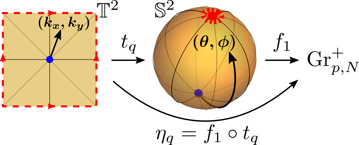 |
A generic oriented total gapped bundle over the Brillouin zone torus is obtained as a pullback by the composition map ,
| (26) |
and according to the diagram
| (27) |
where , and , are bundle maps obtained as the inverse of the pullbacks , and , respectively, and the mapping on the bottom-right is the Plücker embedding of the Grassmannian explained in Sec. VII.4. It follows from the described construction, that the integer determines the isomorphism class of the oriented total gapped bundle, such that . This defines the homomorphism of groups
| (28) |
with , , and .
Finally, writing the oriented total gapped bundle as , the corresponding diagram for the vector subbundle is
| (29) |
[and similarly for ], where is the vector subbundle of the bundle defined over . We emphasize that since the associated total gapped bundle is generated from the pullback by a map to the oriented Grassmannian () it has no nontrivial weak invariants. In other words, the Berry phases over either the occupied and the unoccupied band subspaces are all trivial, even though the base space () contains non-contractible loops.
VII.4 Plücker embedding
We now motivate how to represent the image via a general procedure that would be discussed more explicitly for three-band and four-band models in Secs. VIII and IX. To achieve this, we employ the Plücker embedding which represents the oriented Grassmannian as a -dimensional submanifold of the -th exterior power of (i.e. the -dimensional Euclidean vector space spanned by -component and fully anti-symmetric -vectors). As a result, the image of the Plücker embedding can be generally represented by Kozlov 2000
| (30) |
Here, is the cone of simple (or decomposable) -vectors, i.e. those of the form for some collection of vectors in (not necessarily pairwise orthogonal), and is the unit sphere in with respect to the linear inner product defined on simple -vectors as1111 11 Equivalently, the right-hand side of Eq. (31) is the determinant of a matrix with elements .
| (31) |
where is the permutation group of elements.
The Plücker embedding is defined explicitly as follows. For a given point we take a representative , and we construct as the wedge product of the columns of subframe , that is
| (32) |
Crucially, the -vector in Eq. (32) is invariant under the gauge transformations of the frame , meaning that all choices of the representative of result in the same image . Furthermore, note that is by definition a simple -vector, and it is easy to check that it has a unit norm, implying . The validity of the equality in Eq. (30) is less obvious1212 12 The inverse map, i.e. the one that assigns to any simple -vector with unit norm a unique oriented -plane, can be obtained by considering the decomposition of the matrix representing the -vector., but can be proved Kozlov 2000.
Note that one can similarly define as the exterior product of the eigenvectors of subframe . Although in general (in a similar way as generically ), the two objects are canonically related as Hodge duals, namely . The invariance of and of under gauge transformations with and , and the fact that the images of the two subframes are uniquely related as Hodge duals, together imply that Eq. (32) is a faithful representation of the oriented Grassmannian.
In the following sections, we obtain an explicit parametrization of for and through the Plücker embedding.
Starting from the general parametrization of an element , the task is to find the restriction to the parametrization of an element of the image (corresponding to the generator of the second homotopy group of the Grassmannian), as this provides the parametrization of the subframes and , which directly encode the Hamiltonian . By explicitly solving this problem for and , we derive explicit three-band and four-band tight-binding models for all the homotopy classes.
VII.5 Homotopy classes of total gapped bundles
We argued in Sec. V.4 that two-band subspaces are characterized by the Euler class , while -band subspaces with are characterized by the second SW class, . We will see in Secs. VIII and IX for several concrete examples that the element of the second homotopy group for the oriented total gapped bundle determines the Euler and the second SW classes of both vector subbundles and , depending on for the map [Fig. (3)].
When the classifying space is a product space, i.e. ( being some indexing set), the second homotopy group splits as a direct sum . Thus the map splits accordingly into the components where the indexing set contains the components with a non-trivial . This scenario notably occurs for that is discussed in Sec. IX. Under these circumstances, one needs to replace the base space of the reference total gapped bundle in Eq. (29) by a product , i.e. one copy of for each generator of , and the maps relate . The map from to is characterized by a vector of integers , with each element encoding the map in Eq. (25) to the respective . The composition map then determines the homotopy class (and therefore also the Euler resp. the second SW class of both band subspaces) of the mapping .
VIII Three-band models
We now turn the attention to the specific case of bands, and we deploy the machinery developed in the previous sections in a concrete context. From a physical perspective, we point out that the topology has appeared in numerous physical settings. In particular, for nematic systems the associated topology has been extensively studied Volovik and Mineev 2018; Beekman et al. 2017; Alexander et al. 2012; Liu et al. 2016; Machon and Alexander 2016, as well as non-Hermitian band topology has been related to it Wojcik et al. 2020.
VIII.1 The three-band classifying space
Nontrivial topology can be achieved in a three-band system when a band gap separates a two-band (occupied) subspace and a single-band (unoccupied) subspace (see Table 1). The classifying space of the orientable phases is leading to the homotopy classification of all the topologically nonequivalent phases (see Sec. V). The factor “” here is a convention made such that the value of the topological invariant agrees with the computed Euler class, as we elaborate below.
As explained in Sec. V.3, the associated bundle of the Hamiltonian of an orientable phase can be given an orientation. Therefore, in the following we work with oriented bundles as a mean to build explicit tight-binding models. The classifying space of the oriented phases is (cf. Sec. III.3 and Fig. 2), leading to the homotopy classification with the topological invariant given by an even integer Euler class . The homotopy classes of the orientable phases are then obtained by dropping the orientation, resulting in the topological classification with the reduced Euler class as the topological invariant. We give an explicit example of such a reduction Wojcik et al. 2020 in Appendix D.
We start from an arbitrary element
| (33) |
that is parametrized by three continuous angles (e.g. the Euler angles). Choosing a Cartesian frame of to decompose the eigenvectors, i.e. for , the Plücker embedding of the two-band subspace is given through the bivectors
| (34) | ||||
Note that the expressions in the parentheses correspond to components of , by virtue of the property in Eq. (33). By formally identifying the basis of the three-dimensional Euclidean vector space with the Cartesian frame of via the Hodge dual, i.e. , we get , which is a specific instance of the duality discussed in Sec. VII.4.
We thus infer that spherical coordinates for three-dimensional orthonormal frames defined on provide the desired mapping onto the non-trivial sphere inside the Grassmannian, i.e. we use
| (35) |
with
| (36) | ||||
which correspond respectively to the directions “up”, “south”, and “east” at every point of the sphere. Indeed, , which is invariant under any gauge transformation , represents the oriented plane perpendicular to and, by definition, an element of .
VIII.2 Three-band reference total gapped bundle
Note that is an oriented orthonormal frame of , i.e. of the tangent space at the point of the sphere, and is the basis of the normal space to the point of the sphere. Therefore, these vectors span the tangent bundle , and the normal bundle , respectively. Furthermore, since , the total gapped tautological bundle is topologically equivalent to the couple , so we write
| (37) |
Then, since , the same is true for the pullback bundle
| (38) |
with and .
It is well known through the hairy ball theorem that the tangent bundle of the 2-sphere is non-trivial, namely any global section, (i.e. any smooth tangent vector field) must have zeros associated with a vortex structre. We illustrate this known fact on an example in Fig. 2(c), which displays the eigenvectors of a tight-binding model presented in the next section. The hairy ball theorem is formalized by the Poincaré-Hopf theorem, which states
| (39) |
where is the location of a zero of the vector field , is the winding number of around the zero , and is the Euler characteristic of the sphere Frankel 2011. Thus, any tangent vector field must have two sources of vorticity 1. In the more general context of our classification scheme, the Euler characteristic of the sphere is substituted by the Euler class of the rank-2 subspace of our reference bundle, which however is still by virtue of Eq. (38) [c.f. also to the diagram in Eq. (29)]. We show below that the vortices of the tangent vector field correspond to nodal points within the two-band subspace.
| (a) | |
 | |
 | |
 |
|
| (b) | |
 | |
 | |
 |
 |
 |
| M |
In this context, we emphasize the stable triviality of the tangent bundle of the sphere, i.e. that it becomes trivial upon the direct sum with a trivial bundle. The normal bundle of the sphere is trivial, and the direct sum gives . In other words, the nontrivial tangent bundle (with the non-zero characteristic Euler class ) is trivialized by the trivial normal bundle Hatcher 2001; Hatcher 2003 (resulting in the vanishing characteristic second SW class ). The trivialization (or reduction) of the fragile topology of two-band subspaces upon closing the adjacent energy gap as discussed in Sec. VI.3 can thus be perceived as a fingerprint of the stable triviality of the tangent bundle of the sphere.
VIII.3 Simple model generation
Importantly, we make use of the presented machinery to generate explicit models of fragile topological phases over the Brillouin zone torus for an arbitrary homotopy class (corresponding respectively to Euler class ). As elaborated previously, we first construct explicit models with a specific orientation that are classified by , and then we drop the orientation resulting in a topological classification. The continuous deformations that relate oriented tight-binding Hamiltonians with Euler class are explicitly presented in Appendix D.
For the mapping (cf. Fig. 3) wraps the Brillouin zone torus around the sphere once, and we have . The Hamiltonian representative is then readily given by Bzdušek and Sigrist 2017
| (40) |
where is a identity matrix, is the identity in the single-band unoccupied subspace, and the frame with
| (41) |
for , with defined in Eq. (36) and from Eqs. (25). Sampling over a grid and performing an inverse discrete Fourier transform, we obtain the hopping parameters of a tight-binding model, which we truncate to a few neighbors (see Appendix C and Ref. Bouhon 2020 for more details) without affecting the topological features. Accordingly, we note that while the bands of the Hamiltonian constructed above are flat and the two occupied bands are fully degenerate, these features are lost in our tight-binding models after performing the truncation. Indeed, imposing the perfect flatness and degeneracy results after performing the inverse Fourier transform in an infinite-range hopping amplitudes.
We show in Fig. 2(a) the band structure of the obtained tight-binding model (truncated at two nearest neighbors in both directions of the square lattice, see Appendix C and Ref. Bouhon 2020) that is a representative Hamiltonian for with Euler class . In agreement with the rule , we find nodal points between the two lower bands of Fig. 2(a), two around and two around . Since the pairs of nodes appear very close to each other, we zoom in the neighborhood of the points and M in Fig. 5 to properly resolve them.
We now demonstrate explicitly the equivalence of vector bundles and mentioned below Eq. (38). To achieve this, we transfer the eigenvectors of the band structure in Fig. 2(a) defined over the Brillouin zone torus to two tangent vectors and one normal vector over each point of the sphere. This is done through the mapping as a “pushforward” of vector fields, i.e. for . We thus plot on the right Fig. 2(a) the tangent vector field given by the eigenvectors of the lower energy band of the two-band subspace of the band structure shown on the left of Fig. 2(a). As a global section of the tangent bundle , it can be characterized by invoking the Poincaré-Hopf theorem from Eq. (39). This indicates the equivalence between the Euler characteristic and the Euler class . We also observe that the nodal points of the band structure with fragile topology [left upper panel of Fig. 2(a)] correspond to vortices of the section of [right Fig. 2(a)].
We can repeat the exercise for arbitrary . We show an example of band structure for in Fig. 2(b) with the Euler class . We find nodal points in the two occupied bands, namely 4 on the Brillouin zone boundary and 4 around the point. Owing to the pullback construction, we can force a geometric picture of as the tangent and normal bundles of a generalized surface (not a manifold). Since wraps the sphere -times, we can divide the Brillouin zone into cells that are each mapped onto , i.e. we get a tangent vector field over the sphere for each of the cells. Taken together we can think of it as a tangent field over a surface that wraps on itself with sheets and with the two -fold ramification points and , where the former is the image of (blue point in Fig. 3), and the latter is the image of the boundary of the first Brillouin zone (red point in Fig. 3).
VIII.4 Comment on the “triviality” of
We address here a possible source of confusion concerning the triviality of vector bundles, taking the normal bundle of the sphere, and all the line bundles that are pulled back from it, as an example. Further examples in other dimensions are discussed in Sec. X.2.
The homotopy classification of the total gapped bundle characterizes the (stable or unstable) homotopy classes of all the bands at the same time. In the case of the sphere we have seen that the total bundle is characterized by the second homotopy invariant . The homotopy method is in contrast with the cohomology invariants that characterize the stable topology of a single subbundle at a time, i.e. and . The trivial cohomology class of the normal bundle of the sphere reflects the fact that the vector field generated by over the sphere defines a smooth global section, i.e. is a trivial vector bundle.
However, the same vector field defines a hedgehog structure over the sphere, and as such it cannot be continuously deformed into a constant section, e.g. for all . This is precisely captured by the homotopy invariant of the total gapped bundle which can be obtained as the Skyrmion number of the normal vector field (see Appendix D and Ref. Wojcik et al. 2020). From this perspective, one concludes that the normal bundle of the sphere is non-trivial as it belongs to a different homotopy class than the constant vector field.
We emphasize, crucially, that the statement about the non-triviality of is only true as long as we keep the underlying dimension of Euclidean space (or equivalently the rank of the total bundle ) fixed. The trivial cohomology indicates that if we embed the -sphere in an higher dimensional Euclidean space the normal bundle can be fully trivialized, i.e. the extra dimensions allow a continuous deformation of the hedgehog structure into the constant vector field. The nontrivial homotopy invariant of the normal bundle must thus be interpreted as an unstable homotopy which refines the cohomology classification. The same conclusion applies to all line bundles pulled back from .
IX Four-band models
In this section we study the case, i.e. the classifying space of an orientable band structure with four bands and with a single gap condition that separates an “occupied” two-band subspace from an “unoccupied” two-band subspace. As in the previous section we start from the classification of the oriented phases and then we address the effect of dropping the orientation. We first discuss the parametrization of the classifying space obtained from the Plücker embedding from which representative tight-binding models of all the homotopy classes can be derived. We then study in detail several explicit tight-binding models and we establish the complete list of all topologically nonequivalent phases for . We finally briefly address the stability of the topological invariants under the repartitioning of the bands.
IX.1 Parametrization
The diagonalizing matrix, , underlying the Hamiltonian belongs to and thus can be parametrized by six continuous angles. The exterior product of the occupied states is now a point of the image of the Plücker embedding , i.e. a simple unit bivector. Notably, since the number of unoccupied bands is the same, the Hodge dual also is a unit bivector in the same space . We show in Appendix E that their linear combinations where are two complementary three-dimensional vector spaces of bivectors which partition the second exterior power of (a space of dimension ) into two halves, i.e. . Furthermore , thus () belongs to a unit sphere in (). Therefore, the image of the Plücker embedding is the four-dimensional submanifold with points . The inverse embedding induces a diffeomorphism , implying . We observe that splits into two generators of parametrized by .
Let us now consider the image whose points are bivectors parametrized by a pair of angles (see Appendix E for more details). The inverse embedding induces a parametrization of the four-band diagonalizing matrices
| (42a) | |||
| through the assignment | |||
| (42b) | |||
i.e. there is a reduction from six continuous angles for a generic element to four angles for the representatives . It is worth noting that is nothing but a section of the tautological total gapped bundle . The explicit parametrization depends on the chosen encoding of elements . This is done in Appendix E in terms of the Lie algebra of real and anti-symmetric matrices.
IX.2 Generating the models
Once the parametrization in Eqs. (42) is found, we can readily apply our machinery to generate a tight-binding model corresponding to any homotopy class of . Adapting the discussion from Sec. VII.5 to the present situation, we replace the base space of the reference total gapped bundle by , modifying the scheme in Eq. (27) into
| (43) |
where the pair of integers dictates how many times wraps around each of the two target spheres as we cover the Brillouin zone torus. The map splits into such that wraps around (and wraps around ) exactly once. Then we generate all the topological phases through the pullback of the tautological total gapped bundle, , where . The pair then determines the homotopy invariant , and we simply take .
| (a) | ||
 |
 |
 |
| (b) | ||
 |
 |
 |
| (c) | ||
 |
 |
 |
| (d) | ||
 |
 |
 |
| (e) | ||
 |
 |
 |
We show in the left column of Fig. 6 band structures of truncated tight-binding models (for details see Appendix C and Ref. Bouhon 2020) associated to for different combinations of , which were generated in a similar way as the three-band models discussed in Sec. VIII. By construction, each band structure is composed of two two-band subspaces, and . The topology of each oriented subspace is characterized by the Euler class, i.e. and , which we compute here as a two-band Wilson loop winding Bouhon et al. 2019a (middle column of Fig. 6)1313 13 The Wilson loop winding gives the reduced Euler class . The integer invariant can be obtained from the winding of the Pfaffian of the Wilsonnian Hamiltonian Ref. Bouhon et al. 2019b..
Both Euler classes are directly determined by the numbers . While takes value in a free group, the pair of Euler classes must satisfy the sum rule Bzdušek and Sigrist 2017; Ahn et al. 2019.1414 14 This follows from the sum rule for the second Stiefel-Whitney class of the total bundle, namely . From the data presented in Fig. 6, we conclude that there is the following homomorphism of groups from the homotopy invariants to the cohomology invariants,
| (44) |
We explain in Appendix E how the homomorphism follows from the chosen parametrization of . We emphasize that while the parity of the Euler classes must be equal (by virtue of the Whitney sum formula), their sum does not need to vanish.
As anticipated, we again observe that the number of stable nodal points within each two-band subspace follows , , see the right column of Fig. 6 showing the location of nodal points (black points) of one to the two-band subspaces. This does not prevent accidental pairs of nodal points as is found in Fig. 6(e) which exhibits 8 nodal points in the unoccupied two-band subspace while the minimum of only 6 stable nodal points is expected.
IX.3 Dropping of orientation
The topology of orientable band structures is classified by the free homotopy classes (see Sec. V.3) for which there is no canonical definition of an orientation. Therefore, the orientation assumed so far must be dropped. This has the effect of the following reduction of the homotopy classification of band structures (see Sec. VI.2)
| (46) |
where the quotient set is defined through the equivalence relation given by the automorphism that reverses the orientations of both subbundles and . We give in Appendix F an explicit example of a continuous deformation of the Hamiltonian that reverses the Euler class of oriented subbundles of models with two occupied and two unoccupied bands.
This implies that any two phases with, on the one hand, and, on the other hand, , belong to the same homotopy class, which we write
| (47) |
On the contrary,
| (48) |
Given the sum rule of Euler classes, and given the above reduction, we readily obtain the following list of all equivalence classes of topologically nonequivalent phases that are bounded by , and written in terms of Euler class, i.e.
| (49) |
of which Fig. 6 presents only a subset.
IX.4 Fragile topology of four-band models
We conclude this section by commenting on the fragility through a repartitioning of the bands. Let us start from the band structure with [Fig. 6(d)]. As indicated by their Euler class, the two higher bands are connected by a minimum of zero nodal points, and as such they can be separated by an energy gap [as readily visible in Fig. 6(d)] thus enabling a finer partitioning . Then we can lower the band in energy and close the gap with the block , leading to the new partitioning . The (oriented) classifying space corresponding to the repartitioned bands is thus . Then tells us that the nontrivial fragile topology of the occupied two-band subspace () has been trivialized, in agreement with .
The same conclusion can alternatively be obtained by considering the tangent bundle to the 3-sphere which is associated to the classifying space . We explain in Sec. X that oriented vector subbundles pulled back from , i.e. the tangent bundle of the 3-sphere, are classified by where is the dimensionality of the system. Then, since , the two-dimensional restriction of any vector subbundle pulled back from must be fully trivial.
X Generalizations
We now briefly highlight how our construction can be extended in certain directions, underpinning the generality of the presented geometric framework.
X.1 Band structures with multiple gaps
As a first direction, we can generalize to systems with more bands and with multiple energy gaps, as has been briefly foreshadowed in Secs. VI.1 and VI.2. We discuss here the concrete example of for the orientable phases. In this case the total gapped bundle is composed of three vector subbundles, . First lifting the problem to the oriented bundle, we have
| (50) |
The two-band subspaces are characterized by an Euler class, , , which must satisfy the sum rule , which follows directly from the Whitney sum formula and from the triviality of the total Bloch bundle. There is then a homomorphism from the homotopy invariants to the cohomology invariants,
| (51) |
The classification of orientable phases, as opposed to oriented ones, is then obtained by dropping the orientation. This is obtained by taking the quotient
| (52) |
where the first homotopy group is with elements corresponding to the four Berry phase configurations
| (53) |
After dropping the orientation, we hence obtain the following homotopy equivalence expressed through the Euler class of each two-band subspace, i.e.
| (54) | ||||
While the above results constitute a complete homotopy classification of orientable band structures associated to , the flag manifold has a dimension of which makes explicit parametrization challenging.
X.2 Higher-dimensional fragile topologies
Our construction, relating the nontrivial tangent bundle of the sphere and the nontrivial fragile topological band structures of three-level systems, can be straightforwardly generalized to other dimensions. Indeed, any band structure with occupied bands and one unoccupied band has the classifying space , or when the orientation is artificially fixed. The total tautological bundle is then , where the tautological rank- subbundle is the tangent bundle of the -sphere, , and the tautological line bundle is the normal bundle of the -sphere, .
Fixing as the dimensionality of the system, we focus on the orientable phases (note that the definition of orientability of Sec. IV generalizes to an arbitrary dimension of the base space). Then, generalizing the two-dimensional case discussed in Sec. VIII (), in general the Hamiltonian defines a map where wraps on -times, and is an element of . Any associated total gapped bundle is thus obtained as the pullback bundle with a topology that is classified both by (corresponding to the classification of maps ) and by (for the classification of maps ). We conclude that in general the topology is captured by the direct sum
| (55) |
In the special case , the topology is classified by the single homotopy group , similar to Sec. VII. When , we have and all associated total gapped bundles have a trivial topology. This explains the triviality achieved by the repartitioning of bands as discussed in Sec. IX.4. On the contrary when , we predict a richer classification than the examples studied so far in this work. One well-known example is the Hopf bundle and the associated Hopf insulators obtained for and Moore et al. 2008; Deng et al. 2013; Ünal et al. 2019; Alexandradinata et al. 2019b.
We conclude this section by a generalization of Sec. VIII.4 that addressed the unstable non-trivial homotopy of the normal bundle of the sphere . It is a classical result of algebraic topology that the tangent bundles of the -sphere for are fully parallelizable, i.e. smooth global sections (vector fields) can be formed over these spheres. Nevertheless, since for all ’s, it readily follows from our construction that topologically nontrivial bundles can be obtained as the pullback of parallelizable tangent bundles. This again points to the finer topological content of the homotopy classification as compared to the cohomology (i.e. stable) characterization of vector bundles.
The higher dimensional topologies we are alluding to here will be studied comprehensively elsewhere.
XI Conclusion and discussion
We have provided a geometric perspective on fragile topological phases beyond symmetry indicators, while also addressing structures that emerge when a refined partitioning of bands is taken into account. This topological analysis also underlies the novel braiding properties found in Wu et al. 2019; Bouhon et al. 2019b when nodes of different bands are considered. The framework rests on direct homotopy evaluations of the relevant Grassmannians using a geometrical construction, which involves the so-called Plücker embedding into the more manageable projective exterior product spaces. This construction does not only provide descriptive power, enumerating the possible topologies on a generic footing, but in reverse also allows for a direct construction of rather tractable models displaying the desired topological features. These explicit Hamiltonian models provide a valuable platform to investigate the possible experimental signatures of fragile topology beyond symmetry indicators. In this regard, we point out the very recent Ref. Ünal et al. 2020, in which some of the present authors investigated the expected fingerprints of the 3-band Euler-insulator models of Sec. VIII in cold-atoms setups.
We conclude with outlining prospective theoretical generalizations. Firstly, there are the extensions already outlined in Sec. X, namely the generalization to fragile topology in the presence of multiple bands gaps on the one hand (Sec. X.1), and the generalization to higher-dimensional spaces on the other hand (Sec. X.2). Although in the present work we only consider real-symmetric Hamiltonians, such as in the presence of or symmetry, the finer repartitioning of bands discussed in Sec. VI.1 can similarly be considered for complex Hamiltonians classified by complex flag varieties.
Related to the generalization to higher dimensions, when the third momentum is played by the time direction of a periodic drive, it appears that the language of flag varieties may provide a natural language to describe other classes of topological systems, especially in the case of periodically driven Floquet systems Roy and Harper 2017; Nakagawa et al. 2020; Harper et al. 2020. Here, the periodicity of the quasienergy implies that there is no canonical choice of chemical potential. One therefore often assigns the same importance to all spectral gaps of Floquet systems Sun et al. 2018b, suggesting a very natural application for the language of refined band partitioning developed in Sec. VI.
Another promising application of the refined band partitioning and of fragile topology arises in the context of non-Hermitian models Borgnia et al. 2020; Kawabata et al. 2019; Zhou and Lee 2019, where non-standard gap conditions were recently investigated using homotopy theory Sun et al. 2020; Li and Mong 2019. Indeed, as noted in Sec. VIII, the topology of a generic two-band non-Hermitian Hamiltonian has been shown by Ref. Wojcik et al. 2020 to be essentially equivalent to the fragile topology of -band real-symmetric Hamiltonians discussed here. Furthermore, in analogy with the non-Abelian reciprocal braiding of band nodes in real-symmetric Hamiltonians Wu et al. 2019; Bouhon et al. 2019b, refined band partitioning in non-Hermitian models has been shown to also facilitate noncommutative exchange of exceptional points inside momentum space Zhong et al. 2018.
The final extension, which is of particular importance for the study of materials, concerns the interplay with crystalline symmetries. We have shown in Ref. Bouhon et al. 2019a that a point group of crystalline symmetries can lead to an obstruction on the Wilson loop winding (Euler class) of two-band subspaces. This was proved to be directly rooted in the representation theory of the Wilson loop. All the observations we made here should have a similar natural explanation from the exhaustive topological classification of band structures and their explicit realization. We will report on this in due time at another occasion.
XII Acknowledgements
R.-J. S. acknowledges funding from Trinity college, the Marie Curie programme under EC Grant agreement No. 842901 and the Winton programme at the University of Cambridge. T. B. was supported by an Ambizione Grant No. 185806 from the Swiss National Science Foundation.
Appendix A Geometric and topological properties of Grassmannians
We review here a few basic facts about Grassmannians that motivate the results of their homotopy groups and that allow us to formulate in a rigorous way the action of on in Appendix B.
Let us start from the definition of the Grassmannian in Sec. III.2. is a Lie group and is a Lie subgroup (by Cartan’s closed subgroup theorem Lee 2011), so that the unoriented Grassmannian is a smooth (and closed Hatcher 2003) manifold. Then, representing as the space of (non-oriented) -dimensional hyperplanes passing through the origin in , it readily follows that the Grassmannian is path-connected, and thus connected, as any two hyperplanes (i.e. two points of the Grassmannian) can be smoothly rotated into each other. The same conclusions hold similarly for the oriented Grassmannian.
There is a continuous two-to-one surjective map from the oriented Grassmannian to the unoriented Grassmannian,
| (56) |
where we assume , in particular with (see Eqs. (4) and (6)). The map is a covering map and a covering space of the base space Lee 2011.1515 15 We remark the relative freedom in defining the covering map as we could have shifted the image as with an arbitrary , since there is no favored choice of origin for a Grassmannian. This freedom does not play any role in the topology of Grassmannian though. Therefore, the oriented Grassmannian is the orientable double cover of the unoriented Grassmannian . It is interesting to note that the non-orientability of the connected is a necessary and sufficient condition for the connectedness of , i.e. the orientable double cover is made of a single piece, as it can be readily seen in the example of shown in Fig. 2 (that is to be contrasted e.g. with the double cover group of ). Furthermore, we take for granted that the oriented Grassmannian is simply connected (i.e. Hatcher 2001; Hatcher 2003) which makes it the universal cover of the unoriented Grassmannian Lee 2011.
Further important information on the homotopy of Grassmannians is readily obtained from the lifts of continuous maps through the covering map . The lifting criterion says that every continuous map lifts to a continuous map with , such that the lift is uniquely defined once a reference image point is fixed, e.g. Lee 2011; Hatcher 2001. It further follows that every map projects to a map .
A lift can be composed with an automorphism of the covering map , called a deck transformation, defined by an homeomorphism such that Lee 2011. There are only two possible choices for given a fixed , namely the identity, i.e. with , and the orientation reversal [Eq. (7)], i.e. with . (This freedom plays the role of a gauge symmetry of the gapped Hamiltonians.) Let us summarize the above definitions in one diagram
| (57) |
Since , the set of automorphisms of form the automorphism group of the covering .
The lift of one point, say , is called the fiber and is here given by . Let us transfer the lifting property to the homotopy classes and with the respective base points and . We have and . Fixing the base point of the lifted map, say , we thus have a bijection of homotopy classes leading to the isomorphism Hatcher 2001
| (58) |
This isomorphism lies at the core of our strategy to built homotopy-based tight-binding models in Sec. VII.
We define the action of a nontrivial element (with the base point ) on the fiber in terms of the end point of the lifted paths , i.e. and , called the monodromy action of the fundamental group on the fiber of the covering map. In our case, it is equivalent to the restriction of the deck transformation ‘sr’ to the fiber over a point.
Let us now consider the first homotopy group of the unoriented Grassmannian. Since is connected, there exists a continuous path connecting any element to its reversal partner . By projecting onto , the path defines a non-contractible loop . Inversely, the lift of a non-contractible loop produces an open path in which end points have reversed (subframe) orientation. This directly captures the non-orientability of . (That also characterizes non-orientable vector subbundles over a base loop as discussed in Sec. V.) Furthermore, the lift can be composed with the nontrivial deck transformation ‘’, from which we get the path with and . The open path then projects as . If we now take the composed loop (contrary to the composition of functions, we read the composition of paths/loops from left to right), it lifts to a closed loop which is contractible to a point since . Thus is itself contractible by continuity of the covering map . We conclude that the unoriented Grassmannian has a non-trivial fundamental group Bzdušek and Sigrist 2017. It is actually true in general that the automorphism group of a universal covering is isomorphic to the fundamental group of the space being lifted, i.e. Lee 2011.
We illustrate these properties with the example of the projective plane in Sec. III.3.
Appendix B Action of on
 |
This appendix gives the precise definition of the action of on which then leads to the results of Sec. V.3. For this we use the definition of the first, resp. the second, homotopy groups in terms of continuous functions from the unit interval , resp. continuous functions from the unit square , to a topological space , such that the boundaries , resp. , are mapped to the base point , see Fig. 7 that follows Ref. Hatcher 2001. Importantly, the base point is kept constant for all the maps and the orientation of the unit interval (square), seen as a subspace of the real vector space , transfers to an orientation of the image () within the target space . These allow the definition of composition of homotopies which then induces a group structure on the homotopy equivalence classes () Hatcher 2001. By removing the constraint of a fixed base point we obtain the free homotopy set which may lack a group structure. We show below that this is the case for the unoriented Grassmannian.
In the following we take and .1616 16 We can now motivate the lifting criterion presented in Appendix A. By taking a one-dimensional cross-section of the mapping [Fig. 7], i.e. with and , we find . We thus conclude that the image for any is orientable, and can be lifted to a map into the orientable double cover, i.e. . (The gapped total bundle associated to , interpreted as the classifying map, is thus orientable as well.) Let us define the homotopy Hatcher 2001 as the pre-composition of with the displacement of the base point along the loop as shown in Fig. 8. induces the (right) action of on through the group automorphism
| (59) |
While the homotopy preserves the homotopy classes in the free homotopy set (we write ), it can lead to a change of homotopy classes in . It is however not obvious to see it from the above definition. It turns out that we can derive the effect of the action from the action of on the homotopy class of the lifted map , as done below.
 |
 |
The loop and the sphere image lift respectively to a path and a sphere image [Appendix A]. We now can define the lifted homotopy as the homotopy of the lifted maps, i.e. which is unique by the homotopy lifting property Hatcher 2001. If is a contractible loop in , the lifted loop is then also contractible in (see Appendix A), in which case there is a homotopy and in . On the contrary, for a non-contractible loop , we have seen in Appendix A that it lifts to a path connecting end points of opposite orientation in , which we write () and (). We thus have a based-point-changing homotopy according to the first row of Fig. 9. Since has the base point , it cannot be compared within to which has the base point [Fig. 9]. Applying the orientation reversal (the deck transformation ‘sr’) gives with the base point . Therefore, and can now be compared within .
We thus define the action of on through
| (60) |
according to Fig. 9, which then induces the action of on as
| (61) |
Projecting back onto , we get , since , and thus as expected from Eq. (58).
We now show that acts non-trivially in the case . Before doing so though it is useful to briefly review the cohomology invariants introduced in Sec. V.4 that can be used as indicators of the stable homotopy classes of the lifted map . On the one hand, the Euler class can be used as an indicator of the (stable) homotopy class1717 17 The Euler class is defined for the rank-2 oriented subbundle of the gapped total bundle associated to , i.e. the pullback by of the total tautological bundle , see Sec. VII. , such that the sign defines faithfully the orientation of . In other words, the reversal of the orientation of must also flip the sign of the Euler class, i.e.
| (62) |
On the other hand, the case is stably trivial (i.e. ), and the case is indicated by the second Stiefel-Whitney class which forgets orientation, see Sec. V.4.
The second row of Fig. 9 gives , and from Eq. (62) we find
| (63) |
Since the Euler class is an indicator of the stable homotopy class and from Eq. (58) there is a one-to-one correspondence , we finally conclude
| (64) |
For , we either have or that is indicated by the second Stiefel-Whitney class which is invariant under orientation reversal. Thus, acts nontrivially only when . Since though we can generalize Eq. (64) to every .
Appendix C Tight-binding models
In order to get an explicit tight-binding model, we first sample over a grid in the Brillouin zone and perform an inverse discrete Fourier transform (). This gives us the hopping matrix elements . Typically, the hopping elements decay exponentially and we can truncate them beyond a finite support including a few neighbors around the center . The three-band example with Euler class , and all the four-band examples shown in Sec. IX are truncated beyond the second neighbors in both directions, i.e. for all , while the three-band example with Euler class has been truncated beyond the third neighbors in both directions, i.e. for all .
The implementation in Wolfram Mathematica of the above algorithm is available at Ref. Bouhon 2020. The codes generate three-band, and four-band, tight-binding models for any fixed Euler class through the use of the Plücker embeddings presented in Sec. VIII, and Sec. IX and Appendix E, respectively.
Appendix D Euler class reversal in
For completeness, in this Appendix we reproduce from Ref. Wojcik et al. 2020 the continuous and adiabatic transformation that reverses the Euler class of the two-band oriented subbundle of an orientable gapped three-band model classified by , hence realizing the automorphism of Sec. V.3 (and Appendix B).
Our representative Hamiltonians of orientable gapped three-band systems [cf. Eqs. (25) and (40)] can conveniently be parametrized as Bzdušek and Sigrist 2017
| (65) |
with the unit eigenvector of the single unoccupied band, and .
Since is explicitly invariant under the inversion there is not canonical signed Euler class associated with the Hamiltonian. The indeterminacy can be lifted though by assigning a smooth structure to the vector field , which is allowed by virtue of the triviality of any real line bundle defined over the sphere (see Sec. V.4).
As in Sec. VIII this is achieved by setting Bzdušek and Sigrist 2017 , where defines the number of times wraps around the sphere [cf. Eq. (36)]. The Euler class of the oriented occupied two-band subbundle is then . We have thereby promoted the Hamiltonian Eq. (65) to an oriented total gapped bundle with a well defined Euler class.
Since we are interested in an automorphism of the based homotopy group it is crucial to specify a chosen base point that will serve as a reference for comparing any two elements of the group. Let us fix at the blue pole of the sphere [Fig. 3].
Defining the rotation
| (66) |
for , we obtain a smooth deformation of the Hamiltonian through
| (67) |
which is adiabatic (i.e. it preserves the gap between the eigenvalues) since it can be rewritten as the change of basis, i.e.
| (68) |
Exploiting the gauge freedom of the Hamiltonian (i.e. ), we eventually find
| (69) |
which at preserves the base point of the original Hamiltonian, i.e. . Furthermore, we find
| (70) |
such that the Euler class of is . Therefore, at the transformation realizes the automorphism .
As a conclusion, the above construction defines the continuous deformation of Hamiltonian
| (71) |
with and . Then, keeping track of at the base point through the deformation, i.e. , this defines a non-contractible loop within , i.e. a generator of Wojcik et al. 2020.
Appendix E Plücker embedding for
In this Appendix we derive the explicit Plücker embedding for . We do it starting from the parametrizations of in terms of the Lie algebra of real and anti-symmetric matrices.
E.1 Parametrization of
A matrix can be decomposed as Haber with
| (72) |
where and are arbitrary real antisymmetric matrices, and is a generic matrix in . can be parametrized as Haber
| (73) |
with the angle , where and , and an other angle defined through and . The range of these angles are . A generic matrix can be decomposed as
| (74) |
with the angles and . This results in
| (75) |
We now need the constraints among the six angles, , as to only cover the quotient space . Before doing so, we first review the diffeomorphism of spaces . The readers familiar with the Plücker embedding may jump to the solution Eq. (87).
E.2
We review here the standard result obtained through the Plücker embedding arctic tern 2017. This section follows the argument of arctic tern 2017 with a few more steps.
The Plücker embedding represents the points of the oriented Grassmannian as elements of the second exterior power of , , that is a vector space of dimension spanned by bivectors, i.e. the exterior product () of two vectors of . More specifically, for the image of the Plücker embedding is defined by the solutions to the system
| (76) |
where the norm is defined in terms of a inner product in , see below.
Let us take an oriented orthonormal frame of . There is a bijection between any oriented plane and an element , given that is spanned by the orthonormal frame . The orthogonal complement is then represented by the Hodge dual .
We have . Thus, the -eigenspaces of the Hodge star , which we note and , are composed of elements of the form . These are perpendicular with respect to the exterior and the inner products, i.e. for and , where the inner product of two elements of is defined through with .
Setting , the equation gives , and the equation gives . Combining these we get the relation . Thus, the system Eq. (76) is readily satisfied for with . We conclude that an element of is represented by an element with and .
For we have , such that and split into two orthogonal components each of dimension 3, i.e. . Since are unit bivectors, the spaces are the unit spheres in , i.e. . Since every point of the oriented Grassmannian is represented through the Plücker embedding by a bivector , we conclude that the image of the embedding is .
E.3 From to
The previous section provides the guidelines for the derivation of the constraints Eq. (87) that map the elements of to the elements of .
Choosing a Cartesian frame for , each column vector of reads
| (77) |
We then choose a reference basis for ,
| (78) |
and compute the elements and .
Let us make the following change of basis for ,
| (82) |
which we rewrite as
In the new basis, we then get
| (85) | ||||
| (86) |
i.e. this basis emphasizes that and live in three-dimensional orthogonal complements of the six-dimensional vector space .
The restriction of and to unit spheres is then obtained through
| (87) |
with the spherical angles . Indeed, substituting Eq. (87) we find in the basis ,
The inverse Plücker embedding then gives a bijection,
| (88) |
that we use in Sec. IX for building explicit tight-binding models for all homotopy classes.
Appendix F Euler class reversal in
Let us consider the following transformation for ,
| (89) |
with the rotation
| (90) |
for , and the gauge transformation
| (91) |
We then readily find that applying the Plücker embedding of the previous section to and at , gives
| (92) |
in the basis . Therefore, the winding numbers for are , corresponding to a reversal of Euler class . Choosing the base point at which , the path of left cosets defines a non-contractible loop in , i.e. the generator of .
References
- Qi and Zhang (2011) Xiao-Liang Qi and Shou-Cheng Zhang, “Topological insulators and superconductors,” Rev. Mod. Phys. 83, 1057–1110 (2011).
- Hasan and Kane (2010) M. Z. Hasan and C. L. Kane, “Colloquium: Topological Insulators,” Rev. Mod. Phys. 82, 3045–3067 (2010).
- Schnyder et al. (2008) Andreas P. Schnyder, Shinsei Ryu, Akira Furusaki, and Andreas W. W. Ludwig, “Classification of topological insulators and superconductors in three spatial dimensions,” Phys. Rev. B 78, 195125 (2008).
- Kitaev (2009) A. Kitaev, “Periodic table for topological insulators and superconductors,” AIP Conf. Proc. 1134, 22 (2009).
- Hughes et al. (2011) Taylor L. Hughes, Emil Prodan, and B. Andrei Bernevig, “Inversion-symmetric topological insulators,” Phys. Rev. B 83, 245132 (2011).
- Fu (2011) Liang Fu, “Topological Crystalline Insulators,” Phys. Rev. Lett. 106, 106802 (2011).
- Turner et al. (2012) Ari M. Turner, Yi Zhang, Roger S. K. Mong, and Ashvin Vishwanath, “Quantized response and topology of magnetic insulators with inversion symmetry,” Phys. Rev. B 85, 165120 (2012).
- Slager et al. (2012) Robert-Jan Slager, Andrej Mesaros, Vladimir Juričić, and Jan Zaanen, “The space group classification of topological band-insulators,” Nat. Phys. 9, 98 (2012).
- Juričić et al. (2012) Vladimir Juričić, Andrej Mesaros, Robert-Jan Slager, and Jan Zaanen, “Universal Probes of Two-Dimensional Topological Insulators: Dislocation and Flux,” Phys. Rev. Lett. 108, 106403 (2012).
- Fang et al. (2012a) Chen Fang, Matthew J. Gilbert, and B. Andrei Bernevig, “Bulk topological invariants in noninteracting point group symmetric insulators,” Phys. Rev. B 86, 115112 (2012a).
- Morimoto and Furusaki (2013) Takahiro Morimoto and Akira Furusaki, “Topological classification with additional symmetries from Clifford algebras,” Phys. Rev. B 88, 125129 (2013).
- Shiozaki and Sato (2014) Ken Shiozaki and Masatoshi Sato, “Topology of crystalline insulators and superconductors,” Phys. Rev. B 90, 165114 (2014).
- Chiu et al. (2016) Ching-Kai Chiu, Jeffrey C. Y. Teo, Andreas P. Schnyder, and Shinsei Ryu, “Classification of topological quantum matter with symmetries,” Rev. Mod. Phys. 88, 035005 (2016).
- Slager et al. (2014) Robert-Jan Slager, Andrej Mesaros, Vladimir Juričić, and Jan Zaanen, “Interplay between electronic topology and crystal symmetry: Dislocation-line modes in topological band insulators,” Phys. Rev. B 90, 241403 (2014).
- Bouhon and Sigrist (2014) Adrien Bouhon and Manfred Sigrist, “Current inversion at the edges of a chiral -wave superconductor,” Phys. Rev. B 90, 220511 (2014).
- Slager et al. (2015) Robert-Jan Slager, Louk Rademaker, Jan Zaanen, and Leon Balents, “Impurity-bound states and Green’s function zeros as local signatures of topology,” Phys. Rev. B 92, 085126 (2015).
- Alexandradinata et al. (2014) A. Alexandradinata, Xi Dai, and B. Andrei Bernevig, “Wilson-loop characterization of inversion-symmetric topological insulators,” Phys. Rev. B 89, 155114 (2014).
- Alexandradinata et al. (2016) A. Alexandradinata, Zhijun Wang, and B. Andrei Bernevig, “Topological Insulators from Group Cohomology,” Phys. Rev. X 6, 021008 (2016).
- Bzdušek et al. (2016) Tomáš Bzdušek, QuanSheng Wu, Andreas Rüegg, Manfred Sigrist, and Alexey A. Soluyanov, “Nodal-chain metals,” Nature 538, 75 EP – (2016).
- Slager et al. (2016) Robert-Jan Slager, Vladimir Juričić, Ville Lahtinen, and Jan Zaanen, “Self-organized pseudo-graphene on grain boundaries in topological band insulators,” Phys. Rev. B 93, 245406 (2016).
- Kruthoff et al. (2017) Jorrit Kruthoff, Jan de Boer, Jasper van Wezel, Charles L. Kane, and Robert-Jan Slager, “Topological Classification of Crystalline Insulators through Band Structure Combinatorics,” Phys. Rev. X 7, 041069 (2017).
- Shiozaki et al. (2017) Ken Shiozaki, Masatoshi Sato, and Kiyonori Gomi, “Topological crystalline materials: General formulation, module structure, and wallpaper groups,” Phys. Rev. B 95, 235425 (2017).
- Bouhon and Black-Schaffer (2017) Adrien Bouhon and Annica M. Black-Schaffer, “Global band topology of simple and double Dirac-point semimetals,” Phys. Rev. B 95, 241101 (2017).
- Geilhufe et al. (2017) R. Matthias Geilhufe, Adrien Bouhon, Stanislav S. Borysov, and Alexander V. Balatsky, “Three-dimensional organic Dirac-line materials due to nonsymmorphic symmetry: A data mining approach,” Phys. Rev. B 95, 041103 (2017).
- Po et al. (2017) Hoi Chun Po, Ashvin Vishwanath, and Haruki Watanabe, “Symmetry-based indicators of band topology in the 230 space groups,” Nat. Commun. 8, 50 (2017).
- Bradlyn et al. (2017) Barry Bradlyn, L. Elcoro, Jennifer Cano, M. G. Vergniory, Zhijun Wang, C. Felser, M. I. Aroyo, and B. Andrei Bernevig, “Topological quantum chemistry,” Nature 547, 298 (2017).
- Bzdušek and Sigrist (2017) Tomáš Bzdušek and Manfred Sigrist, “Robust doubly charged nodal lines and nodal surfaces in centrosymmetric systems,” Phys. Rev. B 96, 155105 (2017).
- Slager et al. (2017) Robert-Jan Slager, Vladimir Juričić, and Bitan Roy, “Dissolution of topological Fermi arcs in a dirty Weyl semimetal,” Phys. Rev. B 96, 201401 (2017).
- Bouhon et al. (2018) Adrien Bouhon, Johann Schmidt, and Annica M. Black-Schaffer, “Topological nodal superconducting phases and topological phase transition in the hyperhoneycomb lattice,” Phys. Rev. B 97, 104508 (2018).
- Rhim et al. (2018) Jun-Won Rhim, Jens H. Bardarson, and Robert-Jan Slager, “Unified bulk-boundary correspondence for band insulators,” Phys. Rev. B 97, 115143 (2018).
- Höller and Alexandradinata (2018) J. Höller and A. Alexandradinata, “Topological Bloch oscillations,” Phys. Rev. B 98, 024310 (2018).
- Sun et al. (2018a) Xiao-Qi Sun, Shou-Cheng Zhang, and Tomáš Bzdušek, “Conversion rules for Weyl points and nodal lines in topological media,” Phys. Rev. Lett. 121, 106402 (2018a).
- Slager (2019) Robert-Jan Slager, “The translational side of topological band insulators,” J. Phys. Chem. Solids 128, 24 – 38 (2019), spin-Orbit Coupled Materials.
- Kariyado and Slager (2019) Toshikaze Kariyado and Robert-Jan Slager, “-fluxes, semimetals, and flat bands in artificial materials,” Phys. Rev. Research 1, 032027 (2019).
- Po et al. (2018) Hoi Chun Po, Haruki Watanabe, and Ashvin Vishwanath, “Fragile Topology and Wannier Obstructions,” Phys. Rev. Lett. 121, 126402 (2018).
- Bouhon et al. (2019a) Adrien Bouhon, Annica M. Black-Schaffer, and Robert-Jan Slager, “Wilson loop approach to fragile topology of split elementary band representations and topological crystalline insulators with time-reversal symmetry,” Phys. Rev. B 100, 195135 (2019a).
- Alexandradinata and Höller (2018) A. Alexandradinata and J. Höller, “No-go theorem for topological insulators and high-throughput identification of Chern insulators,” Phys. Rev. B 98, 184305 (2018).
- Bradlyn et al. (2019) Barry Bradlyn, Zhijun Wang, Jennifer Cano, and B. Andrei Bernevig, “Disconnected elementary band representations, fragile topology, and wilson loops as topological indices: An example on the triangular lattice,” Phys. Rev. B 99, 045140 (2019).
- Song et al. (2019) Zhida Song, L. Elcoro, Nicolas Regnault, and B. Andrei Bernevig, “Fragile Phases as Affine Monoids: Full Classification and Material Examples,” (2019), arXiv:1905.03262 [cond-mat.mes-hall] .
- Hwang et al. (2019) Yoonseok Hwang, Junyeong Ahn, and Bohm-Jung Yang, “Fragile topology protected by inversion symmetry: Diagnosis, bulk-boundary correspondence, and Wilson loop,” Phys. Rev. B 100, 205126 (2019).
- Alexandradinata et al. (2019a) A. Alexandradinata, J. Holler, Chong Wang, Hengbin Cheng, and Ling Lu, “Crystallographic splitting theorem for band representations and fragile topological photonic crystals,” (2019a), arXiv:1908.08541 [cond-mat.str-el] .
- Elcoro et al. (2020) Luis Elcoro, Zhida Song, and B. Andrei Bernevig, “Application of the induction procedure and the Smith decomposition in the calculation and topological classification of electronic band structures in the 230 space groups,” (2020), arXiv:2002.03836 .
- Song et al. (2020) Zhi-Da Song, Luis Elcoro, and B. Andrei Bernevig, “Twisted bulk-boundary correspondence of fragile topology,” Science 367, 794–797 (2020).
- Peri et al. (2020) Valerio Peri, Zhi-Da Song, Marc Serra-Garcia, Pascal Engeler, Raquel Queiroz, Xueqin Huang, Weiyin Deng, Zhengyou Liu, B. Andrei Bernevig, and Sebastian D. Huber, “Experimental characterization of fragile topology in an acoustic metamaterial,” Science 367, 797–800 (2020).
- Kane and Mele (2005) C. L. Kane and E. J. Mele, “ topological order and the quantum spin hall effect,” Phys. Rev. Lett. 95, 146802 (2005).
- Ahn et al. (2019) Junyeong Ahn, Sungjoon Park, and Bohm-Jung Yang, “Failure of Nielsen-Ninomiya Theorem and Fragile Topology in Two-Dimensional Systems with Space-Time Inversion Symmetry: Application to Twisted Bilayer Graphene at Magic Angle,” Phys. Rev. X 9, 021013 (2019).
- Wieder and Bernevig (2018) Benjamin J. Wieder and B. Andrei Bernevig, “The axion insulator as a pump of fragile topology,” (2018), arXiv:1810.02373 .
- Kooi et al. (2019) Sander H. Kooi, Guido van Miert, and Carmine Ortix, “Classification of crystalline insulators without symmetry indicators: Atomic and fragile topological phases in twofold rotation symmetric systems,” Phys. Rev. B 100, 115160 (2019).
- Ahn et al. (2018) Junyeong Ahn, Dongwook Kim, Youngkuk Kim, and Bohm-Jung Yang, “Band topology and linking structure of nodal line semimetals with monopole charges,” Phys. Rev. Lett. 121, 106403 (2018).
- Wu et al. (2019) QuanSheng Wu, Alexey A. Soluyanov, and Tomáš Bzdušek, “Non-Abelian band topology in noninteracting metals,” Science 365, 1273–1277 (2019).
- Tiwari and Bzdušek (2020) Apoorv Tiwari and Tomáš Bzdušek, “Non-Abelian topology of nodal-line rings in -symmetric systems,” Phys. Rev. B 101, 195130 (2020).
- Bouhon et al. (2019b) Adrien Bouhon, QuanSheng Wu Wu, Robert-Jan Slager, Hongming Weng, Oleg V. Yazyev Yazyev, and Tomáš Bzdušek, “Non-Abelian Reciprocal Braiding of Weyl Nodes and its Manifestation in ZrTe,” (2019b), arXiv:1907.10611 [cond-mat.mes-hall] .
- Po et al. (2019) Hoi Chun Po, Liujun Zou, T. Senthil, and Ashvin Vishwanath, “Faithful tight-binding models and fragile topology of magic-angle bilayer graphene,” Phys. Rev. B 99, 195455 (2019).
- Cao et al. (2018) Yuan Cao, Valla Fatemi, Shiang Fang, Kenji Watanabe, Takashi Taniguchi, Efthimios Kaxiras, and Pablo Jarillo-Herrero, “Unconventional superconductivity in magic-angle graphene superlattices,” Nature 556, 43–50 (2018).
- Kang and Vafek (2020) Jian Kang and Oskar Vafek, “Non-Abelian Dirac node braiding and near-degeneracy of correlated phases at odd integer filling in magic angle twisted bilayer graphene,” (2020), arXiv:2002.10360 .
- Ünal et al. (2020) F. Nur Ünal, Adrien Bouhon, and Robert-Jan Slager, “Quench dynamics of topological euler class in optical lattices,” (2020), arXiv:2005.03033 .
- Wang et al. (2019) Zhijun Wang, Benjamin J. Wieder, Jian Li, Binghai Yan, and B. Andrei Bernevig, “Higher-order topology, monopole nodal lines, and the origin of large Fermi arcs in transition metal dichalcogenides (),” Phys. Rev. Lett. 123, 186401 (2019).
- Bouhon (2020) Adrien Bouhon, “3-band and 4-band real symmetric tight-binding models with arbitrary Euler class based on the Plücker embedding,” GitHub (2020), publicly available Mathematica code, https://github.com/abouhon/EulerClassTightBinding.
- Yu et al. (2011) Rui Yu, Xiao Liang Qi, Andrei Bernevig, Zhong Fang, and Xi Dai, “Equivalent expression of topological invariant for band insulators using the non-Abelian Berry connection,” Phys. Rev. B 84, 075119 (2011).
- Fang et al. (2012b) Chen Fang, Matthew J. Gilbert, and B. Andrei Bernevig, “Bulk topological invariants in noninteracting point group symmetric insulators,” Phys. Rev. B 86, 115112 (2012b).
- Alexandradinata and Bernevig (2016) A. Alexandradinata and B. Andrei Bernevig, “Berry-phase description of topological crystalline insulators,” Phys. Rev. B 93, 205104 (2016).
- Muechler et al. (2016) Lukas Muechler, A. Alexandradinata, Titus Neupert, and Roberto Car, “Topological Nonsymmorphic Metals from Band Inversion,” Phys. Rev. X 6, 041069 (2016).
- Bouhon and Black-Schaffer (2017) A. Bouhon and A. M. Black-Schaffer, “Bulk topology of line-nodal structures protected by space group symmetries in class AI,” ArXiv e-prints (2017), arXiv:1710.04871 [cond-mat.mtrl-sci] .
- Hatcher (2003) A. Hatcher, Vector Bundles and K-Theory (Unpublished, 2003).
- Panati (2007) Gianluca Panati, “Triviality of Bloch and Bloch-Dirac bundles,” Ann. Henri Poincaré 8, 995Ð1011 (2007).
- Budich and Diehl (2015) Jan Carl Budich and Sebastian Diehl, “Topology of density matrices,” Phys. Rev. B 91, 165140 (2015).
- Milnor and Stasheff (1974) John W. Milnor and James D. Stasheff, Characteristic classes (Princeton University Press, Princeton, New Jersey, 1974).
- Thiang (2016) Guo Chuan Thiang, “On the K-theoretic classification of topological phases of matter,” Annales Henri Poincaré 17, 757–794 (2016).
- Montambaux et al. (2018) Gilles Montambaux, Lih-King Lim, Jean-Noël Fuchs, and Frédéric Piéchon, “Winding Vector: How to Annihilate Two Dirac Points with the Same Charge,” Phys. Rev. Lett. 121, 256402 (2018).
- Gottlieb (2003) Daniel Henry Gottlieb, “Eigenbundles, Quaternions, and Berry’s Phase,” ArXiv e-prints (2003), arXiv:math/0304281 .
- Avron et al. (1983) J. E. Avron, R. Seiler, and B. Simon, “Homotopy and Quantization in Condensed Matter Physics,” Phys. Rev. Lett. 51, 51–53 (1983).
- Kennedy and Guggenheim (2015) Ricardo Kennedy and Charles Guggenheim, “Homotopy theory of strong and weak topological insulators,” Phys. Rev. B 91, 245148 (2015).
- Wojcik et al. (2020) Charles C. Wojcik, Xiao-Qi Sun, Tomáš Bzdušek, and Shanhui Fan, “Homotopy characterization of non-Hermitian hamiltonians,” Phys. Rev. B 101, 205417 (2020).
- Hatcher (2001) A. Hatcher, Algebraic Topology (Cambridge University Press, 2001).
- Sun et al. (2020) Xiao-Qi Sun, Charles C. Wojcik, Shanhui Fan, and Tomáš Bzdušek, “Alice strings in non-Hermitian systems,” Phys. Rev. Research 2, 023226 (2020).
- Zhao and Lu (2017) Y. X. Zhao and Y. Lu, “-Symmetric real Dirac Fermions and Semimetals,” Phys. Rev. Lett. 118, 056401 (2017).
- Ahn and Yang (2019) Junyeong Ahn and Bohm-Jung Yang, “Symmetry representation approach to topological invariants in -symmetric systems,” Phys. Rev. B 99, 235125 (2019).
- Moore et al. (2008) Joel E. Moore, Ying Ran, and Xiao-Gang Wen, “Topological Surface states in Three-Dimensional Magnetic Insulators,” Phys. Rev. Lett. 101, 186805 (2008).
- Deng et al. (2013) D.-L. Deng, S.-T. Wang, C. Shen, and L.-M. Duan, “Hopf insulators and their topologically protected surface states,” Phys. Rev. B 88, 201105 (2013).
- Ünal et al. (2019) F. Nur Ünal, André Eckardt, and Robert-Jan Slager, “Hopf characterization of two-dimensional Floquet topological insulators,” Phys. Rev. Research 1, 022003 (2019).
- Alexandradinata et al. (2019b) A. Alexandradinata, Aleksandra Nelson, and Alexey A. Soluyanov, “The actually robust surface signature of a Hopf insulator: Bulk-to-boundary flow of Berry curvature beyond the anomaly inflow paradigm,” arXiv:1910.10717 (2019b).
- Kozlov (2000) S. E. Kozlov, “Geometry of real grassmann manifolds. Parts I, II.” J. Math. Sci. math/0304281, 2239 (2000).
- Volovik and Mineev (2018) G. E. Volovik and V. P. Mineev, “Investigation of singularities in superfluid He3 in liquid crystals by the homotopic topology methods,” in Basic Notions Of Condensed Matter Physics (CRC Press, 2018) pp. 392–401.
- Beekman et al. (2017) Aron J. Beekman, Jaakko Nissinen, Kai Wu, Ke Liu, Robert-Jan Slager, Zohar Nussinov, Vladimir Cvetkovic, and Jan Zaanen, “Dual gauge field theory of quantum liquid crystals in two dimensions,” Phys. Rep. 683, 1 – 110 (2017), dual gauge field theory of quantum liquid crystals in two dimensions.
- Alexander et al. (2012) Gareth P. Alexander, Bryan Gin-ge Chen, Elisabetta A. Matsumoto, and Randall D. Kamien, “Colloquium: Disclination loops, point defects, and all that in nematic liquid crystals,” Rev. Mod. Phys. 84, 497–514 (2012).
- Liu et al. (2016) Ke Liu, Jaakko Nissinen, Robert-Jan Slager, Kai Wu, and Jan Zaanen, “Generalized Liquid Crystals: Giant Fluctuations and the Vestigial Chiral Order of , , and Matter,” Phys. Rev. X 6, 041025 (2016).
- Machon and Alexander (2016) Thomas Machon and Gareth P. Alexander, “Global defect topology in nematic liquid crystals,” Proc. R. Soc. A 472, 20160265 (2016).
- Frankel (2011) Theodore Frankel, Geometry of Physics (Cambridge University Press, 2011).
- Roy and Harper (2017) Rahul Roy and Fenner Harper, “Periodic table for Floquet topological insulators,” Phys. Rev. B 96, 155118 (2017).
- Nakagawa et al. (2020) Masaya Nakagawa, Robert-Jan Slager, Sho Higashikawa, and Takashi Oka, “Wannier representation of Floquet topological states,” Phys. Rev. B 101, 075108 (2020).
- Harper et al. (2020) Fenner Harper, Rahul Roy, Mark S. Rudner, and S.L. Sondhi, “Topology and Broken Symmetry in Floquet systems,” Annu. Rev. Condens. Matter Phys. 11, 345–368 (2020).
- Sun et al. (2018b) Xiao-Qi Sun, Meng Xiao, Tomáš Bzdušek, Shou-Cheng Zhang, and Shanhui Fan, “Three-Dimensional Chiral Lattice Fermion in Floquet Systems,” Phys. Rev. Lett. 121, 196401 (2018b).
- Borgnia et al. (2020) Dan S. Borgnia, Alex Jura Kruchkov, and Robert-Jan Slager, “Non-Hermitian Boundary Modes and Topology,” Phys. Rev. Lett. 124, 056802 (2020).
- Kawabata et al. (2019) Kohei Kawabata, Ken Shiozaki, Masahito Ueda, and Masatoshi Sato, “Symmetry and Topology in Non-Hermitian Physics,” Phys. Rev. X 9, 041015 (2019).
- Zhou and Lee (2019) Hengyun Zhou and Jong Yeon Lee, “Periodic table for topological bands with non-hermitian symmetries,” Phys. Rev. B 99, 235112 (2019).
- Li and Mong (2019) Zhi Li and Roger S. K. Mong, “Homotopical classification of non-Hermitian band structures,” arXiv:1911.02697 (2019).
- Zhong et al. (2018) Qi Zhong, Mercedeh Khajavikhan, Demetrios N. Christodoulides, and Ramy El-Ganainy, “Winding around non-Hermitian singularities,” Nat. Commun. 9, 4808 (2018).
- Lee (2011) John M. Lee, Introduction to Topological Manifolds, 2nd ed. (Springer, 2011).
- (99) Howard E. Haber, “Parameterization of real orthogonal antisymmetric matrices,” http://scipp.ucsc.edu/~haber/webpage/antiortho.pdf, accessed: 2020-01-07.
- arctic tern (2017) arctic tern, “Second homotopy group of real Grassmannians .” Mathematics Stack Exchange (2017), URL: http://math.stackexchange.com/q/2215495 (version: 2017-04-03).