Adaptive Low-Rank Factorization to regularize shallow and deep neural networks
Abstract
The overfitting is one of the cursing subjects in the deep learning field. To solve this challenge, many approaches were proposed to regularize the learning models. They add some hyper-parameters to the model to extend the generalization; however, it is a hard task to determine these hyper-parameters and a bad setting diverges the training process. In addition, most of the regularization schemes decrease the learning speed. Recently, Tai et al. [1] proposed low-rank tensor decomposition as a constrained filter for removing the redundancy in the convolution kernels of CNN. With a different viewpoint, we use Low-Rank matrix Factorization (LRF) to drop out some parameters of the learning model along the training process. However, this scheme similar to [1] probably decreases the training accuracy when it tries to decrease the number of operations. Instead, we use this regularization scheme adaptively when the complexity of a layer is high. The complexity of any layer can be evaluated by the nonlinear condition numbers of its learning system. The resulted method entitled ‘’AdaptiveLRF” neither decreases the training speed nor vanishes the accuracy of the layer. The behavior of AdaptiveLRF is visualized on a noisy dataset. Then, the improvements are presented on some small-size and large-scale datasets. The preference of AdaptiveLRF on famous dropout regularizers on shallow networks is demonstrated. Also, AdaptiveLRF competes with dropout and adaptive dropout on the various deep networks including MobileNet V2, ResNet V2, DenseNet, and Xception. The best results of AdaptiveLRF on SVHN and CIFAR-10 datasets are 98%, 94.1% F-measure, and 97.9%, 94% accuracy. Finally, we state the usage of the LRF-based loss function to improve the quality of the learning model.
Keywords Neural Network Regularization Model Simplification Matrix Factorization Tensor Factorization.
1 Introduction
In the supervised machine learning, we try to find a learning function to predict the output of a system by considering its inputs. The complexity of a learning function can be defined as [2]:
| (1) |
is complex as much as is great. When the model complexity is high, a small noise in the input causes a great change in the output and the generalization fails and the overfitting occurs. In the case of deep neural networks, because of their intrinsic complexity, the model tends to memorize the samples and the generalization power reduces [3]. To solve this problem, different regularization methods are defined to augment a dynamic noise to the model through the training procedure [4, 5]. One of the most popular techniques is dropout [6] and its family [7, 8, 9, 10, 11, 12]. In these methods, in each iteration a subset of weights of the neural network is selected to train. Some of these methods such as [8, 9], impose small changes on the rest of the weights. This family of methods imposes noise on the weights and does not allow the model to memorize the details of the training dataset.
However, in many regularization techniques, the noise is imposing blindly to all components of the learning model and they do not pay attention to the time and place of the overfitting [13]. This is the reason for the slow convergence in the training of these models. To solve this problem, Abpeikar et al. [14] proposed an expert node in the neural trees to evaluate the overfitting along with the training, and when it is high, they used regularization. Bejani and Ghatee [15] introduced the adaptive regularization schemes including the adaptive dropout and adaptive weight decay to control overfitting in the deep networks. But their methods did not simplify the structure of the network weights and the learning model became complex in many iterations. However, various matrix decomposition methods such as spectral decomposition, nonnegative matrix factorization, and low-rank factorization have been proposed to summarize the information in the matrix (or tensor) [16]. For the application of these methods in the data mining fields, one can note to [17]. It seems that, they are also good options for simplifying matrix weights in deep neural networks. In this regard, we find the following attempts: [18, 19, 20]. In a recent paper, Tai et al. [1] used low-rank tensor decomposition to remove the redundancy in CNN kernels. Also, Bejani and Ghatee [21] derived a theory to regularize deep networks dynamically by using Singular Value Decomposition (SVD).
In continuation of these works, in this paper, we define a new measure based on the condition number of the matrices to evaluate when the overfitting occurs. We also identify which layers of a deep neural network have caused the overfitting problem. To address this problem, we use matrix simplification by decomposing matrices into low-rank matrices. This Low-Rank Factorization that drops out the weights adaptively, is entitled as ‘’AdaptiveLRF”. This method can compete with the popular dropout and in many cases surpasses dropout. These results will be supported by some experiments on small-size and large-scale datasets, separately. We also visualize the behavior of AdaptiveLRF on a noisy dataset. Then, on dataset CIFAR-100, we show the performance of AdaptiveLRF using VGG-19. Finally, the results of AdaptiveLRF are compared with some famous regularization schemes including dropout methods [8, 9, 10, 11, 12], adaptive dropout method [15], weight decay with and without augmentation methods [22, 23, 24, 25].
In what follows, we present some preliminaries in Section 2. In Section 3, the AdaptiveLRF is expressed. In Section 4 we present the empirical studies. The final section ends the paper with a brief conclusion.
2 Preliminaries
The overfitting of a supervised learning model such as a neural network is related to the condition number of the following nonlinear system:
| (2) |
where is the output of the neural network with layers. is the weight matrix (or tensor) of the layer is the number of training samples, and is the pair of the inputs and outputs of the sample. After solving this nonlinear system and finding s, the learning model can be used to predict the output for any unseen data. In numerical algebra, it was shown that the condition number of a system is dependent directly on the stability of the solution [26]. Really, when the condition number is great (very greater than 1) the sensitivity of the system over the noise is very high and so the generalization ability of the learning model decreases significantly. Thus, it is a good idea to evaluate the complexity of the learning model by condition number [21]. The condition number can be defined for linear and nonlinear systems. For a linear system where , , and , the condition number is defined as [26]. Really, when the condition number is great (very greater than 1) the sensitivity of the system over the noise. Also, for the non-linear system where is a non-linear vectorized function, one can use the following formula [27]:
| (3) |
where is Frobenius norm, is parameters of , and is Jacobian matrix of respect to .
2.1 Matrix factorization
In this part, we discuss popular matrix factorization (decomposition) and show their ability to improve the system stability. Consider an arbitrary matrix that is factorized into matrices and . In some instances, LU decomposition, Cholesky decomposition, Singular Value Decomposition (SVD), nonnegative matrix decomposition, binary decomposition, can be used to determine the factors [28]. Now, we focus on the low-rank factorization that approximates any matrix with two lower rank matrices and . To improve the approximation, the following optimization problem can be solved:
| (4) |
When and are two vectors, their ranks are 1 and the matrix is factorized to two matrices with the lowest ranks. We refer to this factorization with LRF. Thus, when LRF factorize it into two matrices and To satisfy 4, we should solve a nonlinear system with variables and equation. See [29] for an implementation.
2.2 Tensor factorization
There are two main approaches to factorize a tensor; explicit and implicit. In the explicit factorization of any tensor , we try to find sets of vectors , and such that approximates , where is the tensor production. By minimizing we can factorize into components [1]. However, the explicit tensor decomposition is an NP-hard problem[30]. Therefore, this type of decomposition is not the best way for the regularization of deep networks. Instead, in implicit factorization, we try to apply the matrix factorization methods directly. To this aim, any tensor is sliced into some matrices and on every matrix, we apply the matrix factorization. The results show the efficiency of this approach for deep learning regularization.
2.3 Visualization of factorization effects
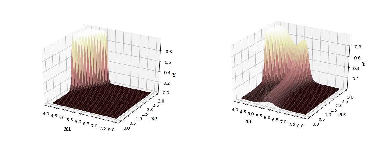
To visualize the effect of matrix and tensor factorization as the regularization method, we designed a test to show how they can improve the learning functions. To this end, we used an artificial noisy dataset based on Iris dataset [31] and constructed a surface to learn these noisy data by a perceptron neural network with 3 hidden layers. Fig.1 shows two surfaces that are trained by the original and noisy datasets separately. As one can see, the learning model is over-fitted because of noisy data. Now, we use LRF on the weighting matrices of the corresponding neural network to regularize this learning model. Fig.2 shows the new surface. It is trivial that the regularized network is more similar to the original learning model that has not destroyed by noisy data. Also, the model is simpler.

3 AdaptiveLRF details
AdaptiveLRF is a regularization technique that is developed for deep neural networks but not limited to these networks. The fundamental steps of this technique are:
- 1.
Detecting the overfitting in continuous steps,
- 2.
Identifying the matrices with great effect on overfitting,
- 3.
Selecting some over-fitted matrices randomly,
- 4.
Using LRF to regularize the over-fitted matrices and the tensors.
To present the details, we need to consider several important points. Noting that, a powerful method for regularization needs to evaluate the overfitting dynamically [15]. When the overfitting is small, the learning procedure can be continued, else, the overfitting should be solved by a regularization method. Such a scheme saves the training speed and increases the generalization ability. The dynamic overfitting can be evaluated b the following criterion:
| (5) |
where is the iteration number. It is worthwhile to note that has an oscillatory behavior and iteratively decreases and increases. Therefore, the average of the last can be considered. is named as patient of regularization. When the overfitting is recognized, the cause of the overfitting must be identified and treated. Because of the layered architecture of deep networks, it is possible to find some of the layers that cause overfitting. The weights of these layers should be regularized to miss some details of data captured by the weighting matrices. However, the major trend of data should be prevented. This leads to a softer surface (as mentioned in Fig.2).
At first glance, finding a sub-set of the layers with the highest effect on overfitting is hard. Instead, we return to the training system and compute the complexity of each layer by its condition number 3. Denote the condition number of layer with . We are ready to regularize the weighting matrices with great But, the experiments show that regularization on every over-fitted matrix increases the processing time. Thus, similar to dropout [6], we define a random test by using distribution. When the produced random parameter is less than the following normalized parameter, we use LRF regularization to simplify the weighting matrices:
| (6) |
To follow the LRF regularization, for the layers with the dense weights and the last convolution layer, the weighting matrices can be approximated by LRF. For the convolution layers with tensor structure, they are sliced to some small matrices with the size of the filter and the number of filters. Then, the LRF approximations are defined on these matrices.
The topic is discussed in the empirical results section. The summarization of the training algorithm with AdaptiveLRF is stated in Algorithm 1.
4 Empirical studies
In this section, the numerical results are shown on AdaptiveLRF and compared them with other regularization methods. Also, we check its power to control the overfitting in the different datasets by using shallow and deep networks. The implementation of AdaptiveLRF can be found here11 1 https://github.com/mmbejani/AdaptiveLRF.
4.1 Effect of condition number in AdaptiveLRF
To present the effect of condition number expressed in Eq. 6 in the performance of AdaptiveLRF, consider the following scenarios:
- 1.
The first layers of the network are used for regularization when the overfitting occurs. In this scenario, the weight matrices of the first layers are factorized by LRF and their approximations are substituted as the new weights matrices.
- 2.
The last layers of the network are used for regularization and so on.
- 3.
This scenario is the combination of the random selection and standard AdaptiveLRF that are presented in Algorithm 1.
To compare these scenarios, VGG-19 network was trained on CIFAR-100. To trace these scenarios, we define the following criterion namely summation of normalized condition number (SNCN):
| (7) |
where is defined in Eq.6 as the condition number of layer . The smaller this criterion in different iterations, the greater the network’s stability against overfitting.
In figures 3 and 4, the performance of the VGG-19 for the presented scenarios are presented. As one can see, the performance of AdaptiveLRF for the third scenario is better compared with the others in terms of SNCN, training loss, and testing loss values.


In addition, one can see the leap of the loss function in training and testing results is different. Two snapshots of them are shown in Fig. 5. These snapshots are extracted from the learning procedure of Wide-Resnet on CIFAR-10. As one can see, the AdaptiveLRF has affected by the parts of the network, where the model is over-fitted. Thus, AdaptiveLRF simplifies the model when the model is over-fitted and has a low affect on the other parts. This means that the useful information is seldom eliminated.


4.2 Performance of AdaptiveLRF on Shallow Networks
In this part, we show the results of AdaptiveLRF on the shallow networks applying different datasets. The used shallow networks have at most 5 layers and the layers are composed of dense layer and one dimension convolution layer. The results of AdaptiveLRF for this network are compared with the case that no regularization is used. Also the results of dropout with are presented. Each experiment is repeated 5 times and their average is presented. The results are shown in Table 1. As one can see, in datasets Arcene, BCWD, and IMDB Reviews, AdaptiveLRF can defeat others. In addition, in datasets BCWD whose levels of overfitting are low, AdaptiveLRF is somewhat weaker than the case of non-regularization. Really, the for these datasets belong to .
| Dataset Name | Regularization | Train A | Train L | Test A | Test L |
| Arcene | None | 99.4% | 74.6% | 0.202 | |
| Dropout (0.1) | 60.6% | 59.2% | 0.406 | ||
| Dropout (0.2) | 60.0% | 59.0% | 0.411 | ||
| Dropout (0.3) | 61.1% | 58.0% | 0.413 | ||
| AdaptiveLRF | 97.4% | 85.8% | 0.125 | ||
| BCWD | None | 98.7% | 95.0% | 0.038 | |
| Dropout (0.1) | 99.8% | 95.3% | 0.037 | ||
| Dropout (0.2) | 93.1% | 90.4% | 0.068 | ||
| Dropout (0.3) | 90.8% | 86.5% | 0.112 | ||
| AdaptiveLRF | 97.6% | 95.6% | 0.032 | ||
| BCWP | None | 98.3% | 76.4% | 0.205 | |
| Dropout (0.1) | 97.1% | 75.0% | 0.229 | ||
| Dropout (0.2) | 95.0% | 71.9% | 0.220 | ||
| Dropout (0.3) | 88.0% | 73.2% | 0.211 | ||
| AdaptiveLRF | 89.2% | 74.6% | 0.210 | ||
| IMDB Reviews | None | 100.0% | 85.3% | 0.396 | |
| Dropout (0.1) | 99.7% | 84.5% | 0.542 | ||
| Dropout (0.2) | 99.7% | 84.5% | 0.542 | ||
| Dropout (0.3) | 99.7% | 84.5% | 0.542 | ||
| AdaptiveLRF | 99.4% | 85.6% | 0.354 |
4.3 Performance of AdaptiveLRF on deep networks
In this part, AdaptiveLRF is evaluated on the different popular standard datasets and CNNs. The performance of AdaptiveLRF is illustrated with augmentation and without augmentation.
4.3.1 Comparison Performance
We compare this method with the other regularization methods including weight decay[32], dropout [6] and adaptive weight decay and adaptive dropout [15]. We use popular networks configuration such as MobileNet V2 [33], ResNet V2 [34], DenseNet [35] and Xception [36]. Also, we augment input images with Cutout method[37]. In all of the experiments, the Adam optimization algorithm are used and the number of maximum epochs is fixed for each dataset, individually. We also use SVHN [38] and CIFAR-10[39] as the datasets. In what follows, we present the results.
4.3.2 SVHN
SVHN is an image dataset containing about 600,000 images for the training and 26,000 images for the testing. We consider 200 epochs and evaluate the performance of the different networks with augmentation and without augmentation in Table 2. The augmentation consists of the following operations:
- •
Rotation between to .
- •
Transition the pixels between to .
- •
Using Cutout with probability [37].
Because of the high number of training samples, the probability of overfitting of the deep models on SVHN dataset is low (The small performance difference between with augmentation and without augmentation shows that). Therefore, as one can see in Table 2 the results when regularization is used and without regularization, is close. Besides, sometimes using a regularization scheme causes that the performance decreases (MobileNet with weight decay). However, AdaptiveLRF can bet all of the regularization schemes because it acts when the overfitting appears, and in this dataset that the overfitting level is so low, AdaptiveLRF affects the model lower than the others, therefore, AdaptiveLRF can reach to the better performance.
| Without Augmentation | ||||||||||||
| AdaptiveLRF | Weight Decay | Dropout | Adaptive WD | Adaptive Dropout | None | |||||||
| A | F | A | F | A | F | A | F | A | F | A | F | |
| MobileNet V2 | 96.8 | 97.0 | 93.3 | 93.4 | 93.0 | 93.1 | 95.8 | 96.0 | 94.7 | 94.9 | 96.6 | 96.6 |
| ResNet V2 | 96.6 | 96.7 | 95.8 | 95.9 | 96.1 | 96.1 | 95.8 | 95.8 | 96.1 | 96.2 | 96.4 | 96.5 |
| DenseNet | 97.8 | 97.9 | 96.5 | 96.6 | 97.1 | 97.1 | 97.0 | 97.2 | 97.3 | 97.4 | 96.4 | 96.4 |
| Xception | 97.9 | 98.0 | 96.5 | 96.6 | 97.1 | 97.2 | 97.3 | 97.3 | 97.2 | 97.3 | 97.2 | 97.4 |
| With Augmentation | ||||||||||||
| MobileNet V2 | 96.8 | 97.0 | 95.4 | 95.5 | 89.1 | 89.4 | 95.6 | 95.7 | 95.2 | 95.3 | 97.2 | 97.2 |
| ResNet V2 | 97.4 | 97.4 | 97.1 | 97.1 | 97.1 | 97.1 | 95.7 | 95.7 | 96.1 | 96.2 | 97.2 | 97.3 |
| DenseNet | 97.9 | 98.0 | 96.9 | 97.0 | 95.1 | 95.3 | 97.2 | 97.4 | 95.6 | 95.7 | 97.6 | 97.7 |
| Xception | 97.9 | 98.0 | 97.4 | 97.4 | 97.2 | 97.4 | 97.4 | 97.5 | 97.6 | 97.7 | 97.6 | 97.7 |
* The A and F are accuracy, F-measure.
4.3.3 CIFAR-10
The CIFAR-10 [39] is smaller than SVHN with the same number of classes. We evaluate and compare AdaptiveLRF with other regularization schemes on this dataset with augmentation and without augmentation. The augmentation strategies for CIFAR-10 is as following:
- •
Rotation between to .
- •
Transition the pixels between to .
- •
Horizontal flip the images by probability 0.5.
- •
Using Cutout with probability [37].
We illustrate the results in Table 3. The reported results are achieved after 200 epochs. As one can see, AdaptiveLRF can overcome the other regularization schemes in most of the cases. Besides, the difference between accuracies when using augmentation is lower than when using raw data. This shows that the level of overfitting is decreased when the data is augmented. However, by decreasing the level of the overfitting the effect of AdaptiveLRF decreases and reaches better performance respect to others.
| Without Augmentation | ||||||||||||
| AdaptiveLRF | Weight Decay | Dropout | Adaptive WD | Adaptive Dropout | None | |||||||
| A | F | A | F | A | F | A | F | A | F | A | F | |
| MobileNet V2 | 75.0 | 75.2 | 71.3 | 71.5 | 74.5 | 74.6 | 71.7 | 71.8 | 74.8 | 74.8 | 70.9 | 71.1 |
| ResNet V2 | 73.9 | 74.1 | 73.5 | 73.7 | 74.6 | 74.6 | 74.6 | 74.6 | 74.7 | 74.9 | 72.7 | 72.9 |
| DenseNet | 75.1 | 75.1 | 74.1 | 74.1 | 75.3 | 75.8 | 74.6 | 74.8 | 75.3 | 75.5 | 73.8 | 73.9 |
| Xception | 75.7 | 75.8 | 73.5 | 73.6 | 74.0 | 74.1 | 74.5 | 74.5 | 74.5 | 74.7 | 71.8 | 71.0 |
| With Augmentation | ||||||||||||
| MobileNet V2 | 91.9 | 92.3 | 91.6 | 91.6 | 91.7 | 91.8 | 91.8 | 91.9 | 91.8 | 92.0 | 91.1 | 91.4 |
| ResNet V2 | 92.5 | 92.5 | 92.3 | 92.6 | 92.5 | 92.6 | 92.4 | 92.5 | 92.5 | 92.7 | 92.1 | 92.3 |
| DenseNet | 94.0 | 94.1 | 93.0 | 93.2 | 93.5 | 93.5 | 93.2 | 93.2 | 93.8 | 94.0 | 93.0 | 93.0 |
| Xception | 91.5 | 91.7 | 90.7 | 90.8 | 91.8 | 92.0 | 91.1 | 91.2 | 91.7 | 92.0 | 91.7 | 92.0 |
* The A, F are accuracy and F-measure.
5 An improvement on AdaptiveLRF by the aid of LRF-based loss function
The results showed that AdaptiveLRF prefers on the other regularizers for shallow networks and can compete with other adaptive dropout variations. However, the results of AdaptiveLRF in the deep networks were not the best when the model complexity is high. Recently, Bejani and Ghatee [21] proved a new theory for adaptive SVD regularization (ASR). They used the following loss function to accelerate the convergence of the learning problem:
| (8) |
where denotes the synaptic weights and the bias vector of a neural network and is estimated by the best synaptic weights on the validation dataset. is used for regularization. They minimized this loss function by using their SVD approximation of . Instead, we can use LRF to approximate this term. Thus, we can use the following ‘’LRF-based loss function” in our training model:
| (9) |
Based on the initial results, this modification can improve the quality of learning for different deep neural networks. We will present the details of this experiments soon.
6 Conclusion and future directions
In this paper, we discussed the effects of an adaptive low-rank factorization for neural network regularization entitled AdaptiveLRF. This regularization scheme was not implemented for all layers, which is different from [1]. Instead, the conditional number of the synaptic weights for each layer was evaluated and when it was high, the low-rank approximation of the matrices was substituted. This idea was used to retrieve the information of synaptic weights. The proposed AdaptiveLRF can find a stable solution for the learning problem. We showed the results of this scheme on two categories of shallow and deep neural networks. The results showed that AdaptiveLRF prefers on the other regularizers for shallow networks and can compete with other adaptive dropout variations. However, the results of AdaptiveLRF in the deep networks can be improved by using an adaptive plan similar to ASR [21]. We will present the results of AdaptiveLRF together adaptive LRF-based loss function in future work. Also, overfitting is very important in many machine learning branches and it is necessary to solve them by using context knowledge. The effects of AdaptiveLRF for shallow and deep neural networks in these branches should be evaluated. For future works, one can focus on AdaptiveLRF for solving overfitting in neural networks that are used for feature extraction [40], sensors fusion [41, 42], data visualization [15], and ensemble learning [43]. Since, in [5] the importance of overfitting in transportation problems has been highlighted, we encourage the researchers to implement AdaptiveLRF in the transportation problems [44].
References
- [1] Cheng Tai, Tong Xiao, Yi Zhang, Xiaogang Wang, et al. Convolutional neural networks with low-rank regularization. 4th International Conference on Learning Representations (ICLR), 2016.
- [2] Demyanov Sergey. Regularization Methods for Neural Networks and Related Models. PhD thesis, Department of Computing and Information Systems, The University of Melbourne, 2015.
- [3] Gavin C Cawley and Nicola LC Talbot. Preventing over-fitting during model selection via bayesian regularisation of the hyper-parameters. Journal of Machine Learning Research, 8(Apr):841–861, 2007.
- [4] Mohammad Mahdi Bejani and Mehdi Ghatee. Overfitting control in shallow and deep neural networks: A systematic review. Artificial Intelligence Review, Submitted in Second Review, 2020.
- [5] Mohammad Mahdi Bejani and Mehdi Ghatee. Regularized deep networks in intelligent transportation systems: A taxonomy and a case study. arXiv preprint arXiv:1911.03010, pages 1–8, 2019.
- [6] Nitish Srivastava, Geoffrey Hinton, Alex Krizhevsky, Ilya Sutskever, and Ruslan Salakhutdinov. Dropout: a simple way to prevent neural networks from overfitting. The Journal of Machine Learning Research, 15(1):1929–1958, 2014.
- [7] Li Wan, Matthew Zeiler, Sixin Zhang, Yann Le Cun, and Rob Fergus. Regularization of neural networks using dropconnect. In International Conference on Machine Learning, pages 1058–1066, 2013.
- [8] Guoliang Kang, Jun Li, and Dacheng Tao. Shakeout: A new approach to regularized deep neural network training. IEEE transactions on pattern analysis and machine intelligence, 40(5):1245–1258, 2018.
- [9] Najeeb Khan, Jawad Shah, and Ian Stavness. Bridgeout: stochastic bridge regularization for deep neural networks. arXiv preprint arXiv:1804.08042, 2018.
- [10] David Krueger, Tegan Maharaj, János Kramár, Mohammad Pezeshki, Nicolas Ballas, Nan Rosemary Ke, Anirudh Goyal, Yoshua Bengio, Aaron Courville, and Chris Pal. Zoneout: Regularizing rnns by randomly preserving hidden activations. arXiv preprint arXiv:1606.01305, 2016.
- [11] Gustav Larsson, Michael Maire, and Gregory Shakhnarovich. Fractalnet: Ultra-deep neural networks without residuals. arXiv preprint arXiv:1605.07648, 2016.
- [12] Salman H Khan, Munawar Hayat, and Fatih Porikli. Regularization of deep neural networks with spectral dropout. Neural Networks, 110:82–90, 2019.
- [13] Elham Abbasi, Mohammad Ebrahim Shiri, and Mehdi Ghatee. A regularized root–quartic mixture of experts for complex classification problems. Knowledge-Based Systems, 110:98–109, 2016.
- [14] Shadi Abpeikar, Mehdi Ghatee, Gian Luca Foresti, and Christian Micheloni. Adaptive neural tree exploiting expert nodes to classify high-dimensional data. Neural Networks, 124:20–38, 2020.
- [15] Mohammad Mahdi Bejani and Mehdi Ghatee. Convolutional neural network with adaptive regularization to classify driving styles on smartphones. IEEE Transactions on Intelligent Transportation Systems, 2019.
- [16] Panagiotis Symeonidis and Andreas Zioupos. Matrix and Tensor Factorization Techniques for Recommender Systems, volume 1. Springer, 2016.
- [17] Andrew Y Ng, Michael I Jordan, and Yair Weiss. On spectral clustering: Analysis and an algorithm. In Advances in neural information processing systems, pages 849–856, 2002.
- [18] Emily L Denton, Wojciech Zaremba, Joan Bruna, Yann LeCun, and Rob Fergus. Exploiting linear structure within convolutional networks for efficient evaluation. In Advances in neural information processing systems, pages 1269–1277, 2014.
- [19] Max Jaderberg, Andrea Vedaldi, and Andrew Zisserman. Speeding up convolutional neural networks with low rank expansions. arXiv preprint arXiv:1405.3866, 2014.
- [20] Vadim Lebedev, Yaroslav Ganin, Maksim Rakhuba, Ivan Oseledets, and Victor Lempitsky. Speeding-up convolutional neural networks using fine-tuned cp-decomposition. arXiv preprint arXiv:1412.6553, 2014.
- [21] Mohammad Mahdi Bejani and Mehdi Ghatee. Theory of adaptive svd regularization for deep neural networks. Neural Networks, 2020, Submitted.
- [22] Logan Engstrom, Brandon Tran, Dimitris Tsipras, Ludwig Schmidt, and Aleksander Madry. A rotation and a translation suffice: Fooling cnns with simple transformations. arXiv preprint arXiv:1712.02779, 2017.
- [23] Arkadiusz Kwasigroch, Agnieszka Mikołajczyk, and Michał Grochowski. Deep convolutional neural networks as a decision support tool in medical problems–malignant melanoma case study. In Polish Control Conference, pages 848–856. Springer, 2017.
- [24] Michał Wąsowicz, Michał Grochowski, Marek Kulka, Agnieszka Mikołajczyk, Mateusz Ficek, Katarzyna Karpieńko, and Maciej Cićkiewicz. Computed aided system for separation and classification of the abnormal erythrocytes in human blood. In Biophotonics—Riga 2017, volume 10592, page 105920A. International Society for Optics and Photonics, 2017.
- [25] Adrian Galdran, Aitor Alvarez-Gila, Maria Ines Meyer, Cristina L Saratxaga, Teresa Araújo, Estibaliz Garrote, Guilherme Aresta, Pedro Costa, Ana Maria Mendonça, and Aurélio Campilho. Data-driven color augmentation techniques for deep skin image analysis. arXiv preprint arXiv:1703.03702, 2017.
- [26] Biswa Nath Datta. Numerical linear algebra and applications, volume 116. Siam, 2010.
- [27] Lloyd N Trefethen and David Bau III. Numerical linear algebra, volume 50. Siam, 1997.
- [28] Lars Eldén. Matrix methods in data mining and pattern recognition, volume 15. Siam, 2019.
- [29] Nimfa. https://github.com/mims-harvard/nimfa. Accessed: 2020-02-10.
- [30] Christopher J Hillar and Lek-Heng Lim. Most tensor problems are np-hard. Journal of the ACM (JACM), 60(6):45, 2013.
- [31] Edgar Anderson. The species problem in iris. Annals of the Missouri Botanical Garden, 23(3):457–509, 1936.
- [32] Anders Krogh and John A Hertz. A simple weight decay can improve generalization. In Advances in neural information processing systems, pages 950–957, 1992.
- [33] Mark Sandler, Andrew Howard, Menglong Zhu, Andrey Zhmoginov, and Liang-Chieh Chen. Mobilenetv2: Inverted residuals and linear bottlenecks. In Proceedings of the IEEE Conference on Computer Vision and Pattern Recognition, pages 4510–4520, 2018.
- [34] Kaiming He, Xiangyu Zhang, Shaoqing Ren, and Jian Sun. Identity mappings in deep residual networks. In European conference on computer vision, pages 630–645. Springer, 2016.
- [35] Gao Huang, Zhuang Liu, Laurens Van Der Maaten, and Kilian Q Weinberger. Densely connected convolutional networks. In Proceedings of the IEEE conference on computer vision and pattern recognition, pages 4700–4708, 2017.
- [36] François Chollet. Xception: Deep learning with depthwise separable convolutions. In Proceedings of the IEEE conference on computer vision and pattern recognition, pages 1251–1258, 2017.
- [37] Terrance DeVries and Graham W Taylor. Improved regularization of convolutional neural networks with cutout. arXiv preprint arXiv:1708.04552, 2017.
- [38] Yuval Netzer, Tao Wang, Adam Coates, Alessandro Bissacco, Bo Wu, and Andrew Y Ng. Reading digits in natural images with unsupervised feature learning. In NIPS Workshop on Deep Learning and Unsupervised Feature Learning, 2011.
- [39] Alex Krizhevsky, Geoffrey Hinton, et al. Learning multiple layers of features from tiny images. 2009.
- [40] Ali Pashaei, Mehdi Ghatee, and Hedieh Sajedi. Convolution neural network joint with mixture of extreme learning machines for feature extraction and classification of accident images. Journal of Real-Time Image Processing, pages 1–16, 2019.
- [41] Mohammad Mahdi Bejani and Mehdi Ghatee. A context aware system for driving style evaluation by an ensemble learning on smartphone sensors data. Transportation Research Part C: Emerging Technologies, 89:303–320, 2018.
- [42] Hamid Reza Eftekhari and Mehdi Ghatee. Hybrid of discrete wavelet transform and adaptive neuro fuzzy inference system for overall driving behavior recognition. Transportation Research Part F: Traffic Psychology and Behaviour, 58:782–796, 2018.
- [43] Shadi Abpeykar, Mehdi Ghatee, and Hadi Zare. Ensemble decision forest of rbf networks via hybrid feature clustering approach for high-dimensional data classification. Computational Statistics & Data Analysis, 131:12–36, 2019.
- [44] Mehdi Ghatee. Smartphone-based systems for driving evaluation. Smartphones Recent Innov. Appl, pages 143–222, 2019.