Why and when pausing is beneficial in quantum annealing

We write the single qubit annealing Hamiltonian in the form

$$H_{\mathrm{S}}(s)=-\frac{1}{2}\big[A(s)Z+B(s)X\big]\ ,$$

(1)

where $s=t/t_{f}$ is the dimensionless instantaneous time, $t$ is the actual time, $t_{f}$ is the total anneal time, and $A(s)$ and $B(s)$ are the annealing schedules. Note that we permuted the Pauli matrices $X$ and $Z$ of the conventional single qubit annealing Hamiltonian in order to have the same expression for both the single qubit and projected TLS cases. After transforming to the adiabatic frame Munoz-Bauza et al. 2019, the dimensionless interaction picture Hamiltonian becomes:

$$\tilde{H}_{\mathrm{S}}\pqty{s}=\frac{1}{2}\pqty{\dv{\theta}{s}Y-t_f\Omega\pqty{s}Z}\ ,$$

(2)

where $\Omega(s)$ and $\theta(s)$ are a reparameterization of the annealing schedules: $A(s)=\Omega(s)\cos\theta(s)$ and $B(s)=\Omega(s)\sin\theta(s)$. (see Appendix A for a detailed explanation). We call $\theta(s)$ the annealing angle and $\dot{\theta}(s)$ the angular progression. The term $\dot{\theta}Y/2$ has its origin as a geometric phase Vinci and Lidar 2017a. Loosely, $\Omega(s)$ corresponds to the time-dependent gap and $\mathrm{d}\theta/\mathrm{d}s$ corresponds to how fast/slow the Hamiltonian changes. For a typical single qubit annealing process, the boundary condition $\theta(0)=0$ and $\theta(1)=\pi/2$ needs to be satisfied (noticing that in Eq. (1) we permuted the Pauli $X$ and $Z$ matrices in the standard notation).

For general multi-qubit annealing, the Hamiltonian is

$$H_{\mathrm{S}}(s)=A(s)H_{\mathrm{d}}+B(s)H_{\mathrm{p}}=\sum_{n}E_{n}\pqty{s}\outerproduct{n(s)}{n(s)}\ .$$

(3)

where $\Bqty{\ket{n\pqty{s}}}$ is the instantaneous energy eigenbasis and $E_{n}\pqty{s}$ are the instantaneous energies. $H_{\mathrm{d}}$ and $H_{\mathrm{p}}$ are the driver and problem Hamiltonian, respectively. Henceforth we assume that $H_{\mathrm{S}}=(H_{\mathrm{S}})^{T}$, i.e., that $H_{\mathrm{S}}(s)$ is real for all $s$. The system density matrix can be written in the instantaneous energy eigenbasis:

$$\rho\pqty{s}=\sum_{nm}\rho_{nm}\outerproduct{n}{m}\ .$$

(4)

We call the associated matrix $\tilde{\rho}=\bqty{\rho_{nm}}$ the density matrix in the adiabatic frame, and show in Appendix B that it obeys the von Neumann equation $\dot{\tilde{\rho}}=-i\commutator{\tilde{H}}{\tilde{\rho}}$ with the effective Hamiltonian

$$\tilde{H}=\begin{pmatrix}t_{f}E_{0}&-i\innerproduct{0}{\dot{1}}&\dots\\ i\innerproduct{0}{\dot{1}}&t_{f}E_{1}&\dots\\ \vdots&&\ddots\end{pmatrix}$$

(5)

If we truncate the effective Hamiltonian (5) to the lowest two energy levels and shift it by a constant term, we find:

$$\tilde{H}_{2}=\innerproduct{0}{\dot{1}}Y-\frac{t_{f}\Omega\pqty{s}}{2}Z,$$

(6)

where $\Omega(s)=E_{1}-E_{0}$ is the energy gap between the lowest two energy levels. We call this the projected TLS Hamiltonian. An alternative way to derive this effective Hamiltonian is via the well-known adiabatic intertwiner (see, e.g., Ref. Rezakhani et al. 2010). This TLS approximation is valid when (i) there is a large gap separating the two-level subspace from higher excited state (where “large” is in the sense of the adiabatic theorem Jansen et al. 2007), and (ii) the geometric terms connecting the two-level subspace to the higher levels in the adiabatic frame are negligible Vinci and Lidar 2017b. One may also invoke the Schrieffer-Wolff transformation to establish similar conditions Bravyi et al. 2011; Consani and Warburton 2020.

Since the annealing Hamiltonian [Eq. (3)] is real, $\innerproduct{0}{\dot{1}}$ in Eq. (5) is also real. This effective Hamiltonian is equivalent to Eq. (2) with $\innerproduct{0}{\dot{1}}$ playing the role of $\dot{\theta}/2$. Thus, we can define the angular progression as $\dot{\theta}=2\innerproduct{0}{\dot{1}}$ for the projected TLS. Having done so, a general TLS Hamiltonian can also be written as Eq. (2), where the annealing angle $\theta$ in the general case does not need to satisfy the same boundary condition as in the single qubit case.

We call an instance “easy” when a high ground state probability is achieved within an annealing time that is much shorter than the timescale set by the inverse of the minimum gap along the anneal (we refer to this as the “heuristic” adiabatic condition; it is not to be confused with the rigorous adiabatic condition, which provides a sufficient condition for convergence to the ground state Jansen et al. 2007; Lidar et al. 2009). Conversely, we call an instance “hard” when the ground state probability is low for such an annealing time.

Our strategy is to create toy models that share the same features as certain known hard examples for quantum annealing Dickson et al. 2013; Passarelli et al. 2019. By closely examining those problems, we identify one crucial characteristic they share: a sharp peak in the angular progression appears at the minimum gap, along with a $\pi$ jump of the annealing angle $\theta$ (see Appendix C where these examples are illustrated).

We take a reverse engineering approach by first specifying the analytic form of the gap $\Omega(s)$ and angular progression $\dot{\theta}\pqty{s}$ in the adiabatic frame. The gap is parametrized as a Gaussian in the form

$$\Omega(s)=E_{0}\pqty{1-\pqty{1-\Delta}e^{-\frac{(s-\mu_g)^2}{2\alpha^2_g}}}\ ,$$

(7)

where the parameters $\Delta$, $\mu_{g}$ and $\alpha_{g}$ respectively control the gap size, position and width. The angular progression can also be chosen as Gaussian

$$\dot{\theta}(s)=Ce^{-\frac{(s-\mu_{\theta})^{2}}{2\alpha_{\theta}^{2}}}$$

(8)

with position and width parameter $\mu_{\theta}$ , $\alpha_{\theta}$. The normalization constant $C$ is chosen according to the boundary condition. We will discuss both the single qubit and projected TLS cases.

As a consequence of the aforementioned boundary conditions $\theta(0)=0$ and $\theta(1)=\pi/2$. the normalization constant is

$$C=\sqrt{\frac{\pi}{2}}\frac{1}{2\alpha_{\theta}}\ ,$$

(9)

and the annealing angle resulting from Eq. (8) is

$$\theta(s)=\frac{\pi}{4}\bigg[\erf\left(\frac{\mu_{\theta}}{2\alpha_{\theta}}\right)+\erf\left(\frac{s-\mu_{\theta}}{\sqrt{2}\alpha_{\theta}}\right)\bigg]\ .$$

(10)

In order to ensure the hardness of the problem and monotonic schedules, we need to overlap the peak region of $\dot{\theta}$ and the minimum gap, i.e., $\mu_{\theta}\approx\mu_{g}$. In such a region, the diabatic term is much larger than the adiabatic term and the Landau-Zener transition is strong. A choice of such schedules is illustrated in Fig. 1. It is important to note that, in this construction, the hardness of the problem is not solely determined by the minimum gap $\Delta$. Indeed, the rigorous adiabatic condition involves the derivative of the Hamiltonian as well Jansen et al. 2007; Lidar et al. 2009. An example of an easy instance with a small minimum gap is given in Appendix D.

The boundary conditions for the projected TLS are different from the single qubit case because there is no simple relation between the schedules and the annealing angle. However, a common feature of the small gap instances Dickson et al. 2013; Passarelli et al. 2019 is a localized pulse of angular progression that is present at the minimum gap. Also, this pulse induces a step-function like $\pi$ shift of the annealing angle across this region, leading to a near-perfect Landau-Zener transition. The simplest toy model we can construct is to keep the Gaussian form of the gap [Eq. (7)] and angular progression [Eq. (8)] but use a different boundary condition $\theta(0)=0$ and $\theta(1)=\pi$, which comes from the examination of both the $p$-spin model Passarelli et al. 2019 and the D-Wave $16$-qubit gadget problem Dickson et al. 2013. In this case, the normalization constant becomes $C=\sqrt{\pi}/\sqrt{2}\alpha_{\theta}$.

However, we stress that the core of this construction is the angular progression pulse at the minimum gap. There is no constraint on $\dot{\theta}\pqty{s}$ at other $s$ as long as the system can follow its eigenstates before and after the pulse. In fact, in the problem studied in Ref. Dickson et al. 2013, the annealing angle first gradually decreases to a non-zero value before the $\pi$ jump (see Appendix C).

Before proceeding, we define the bath correlation function

$$C_{\alpha\alpha^{\prime}}(s,s^{\prime})=\Tr[\mathcal{B}_{\alpha}(s)\mathcal{B}_{\alpha^{\prime}}\pqty{s'}\rho_{\mathrm{B}}]=C_{\alpha}^{*}(s^{\prime},s)$$

(16)

in terms of the rotated $\mathcal{B}_{\alpha}$ operator

$$\mathcal{B}_{\alpha}(s)=U^{\dagger}_{\mathrm{B}}(s)\mathcal{B}_{\alpha}U_{\mathrm{B}}(s)\ ,$$

(17)

where $U_{\mathrm{B}}(s)=\exp[-it_{f}H_{\mathrm{B}}s]$ is the free bath evolution. We call a set of $\Bqty{\mathcal{B}_\alpha(s)}_{\alpha}$ independent if $C_{\alpha\alpha^{\prime}}(s,s^{\prime})=\delta_{\alpha\alpha^{\prime}}C_{\alpha}(s,s^{\prime})$ $\forall\alpha,\alpha^{\prime}$, and identical if $C_{\alpha}(s,s^{\prime})=C(s,s^{\prime})$ $\forall\alpha$.

By assuming $\Bqty{\mathcal{B}_\alpha(s)}_{\alpha}$ are independent, the Redfield equation in the adiabatic frame can be shown to be Munoz-Bauza et al. 2019:

	$\displaystyle\dot{\rho}_{S}(s)$	$\displaystyle=-i\commutator{H_\mathrm{S}(s)}{{\rho}_S(s)}$		(18)
		$\displaystyle\qquad-\sum_{\alpha}(g_{\alpha}t_{f})^{2}\commutator{S_\alpha\pqty{s}}{\Lambda_{\alpha}(s)\rho_S(s)}+\textrm{h.c.}\ ,$

where

$$\Lambda_{\alpha}(s)=\int_{0}^{s}\differential{s'}C_{\alpha}(s,s^{\prime})U(s,s^{\prime})S_{\alpha}\pqty{s'}U^{\dagger}(s,s^{\prime})\ ,$$

(19)

and

$$U(s,s^{\prime})=T_{+}\exp{-it_f\int_{s'}^s H_\mathrm{S}(s'') \dd{s''}}\ ,$$

(20)

and $T_{+}$ denotes time-ordering. An important observation is that, after moving to the adiabatic frame, the transformed system Hamiltonian [Eq. (2)] has a different gap than the original one [Eq. (1)], due to the rescaling by $t_{f}$. We define the new gap (in energy units) in the adiabatic frame as

$$\Delta\pqty{s}=\sqrt{\dot{\theta}^{2}\pqty{s}/t_{f}^{2}+\Omega^{2}\pqty{s}}\ .$$

(21)

From our construction of $\Omega\pqty{s}$ and $\dot{\theta}\pqty{s}$ [Eqs. (7) and (8)], it follows that at the minimum gap point of $s=\alpha_{g}$, $\Delta\pqty{s}$ is large. As a consequence, we can safely apply the rotating wave approximation (RWA) with the adiabatic frame Redfield Eq. (18) without worrying about the presence of a small gap. After the RWA, Eq. (19) becomes

	$\displaystyle\dot{\rho}_{S}$	$\displaystyle=-i\commutator{H_\mathrm{S}\pqty{s}+H_{\mathrm{LS}}}{{\rho}_S}$
		$\displaystyle\qquad-\Gamma_{\mathrm{d}}\big(\rho_{ba}\outerproduct{b}{a}+\rho_{ab}\outerproduct{a}{b}\big)$		(22)
		$\displaystyle\qquad+\Gamma_{\mathrm{t}}\pqty{\rho_{aa}-e^{-\beta\Delta}\rho_{bb}}\big(\outerproduct{b}{b}-\outerproduct{a}{a}\big)\ ,$

where $\rho_{ab}=\matrixelement{a}{\rho_S}{b}$ with $\{\ket{a},\ket{b}\}$ being the ground and excited states of $H_{\mathrm{S}}\pqty{s}$. All quantities in Eq. (22) are $s$-dependent, and the effective dephasing and thermalization rates $\Gamma_{\mathrm{d}}$ and $\Gamma_{\mathrm{t}}$, respectively, are given by Munoz-Bauza et al. 2019:¹¹ 1 The expression we arrive at here for $\Gamma$ here is slightly different from Ref. Munoz-Bauza et al. 2019 since here the RWA is done in the adiabatic frame, while in Ref. Munoz-Bauza et al. 2019 the RWA is done in an additional rotating frame.

	$\displaystyle\Gamma_{\mathrm{d}}\pqty{s}$	$\displaystyle=\frac{t_{f}}{2}\Gamma_{\mathrm{t}}\pqty{s}\big(1+e^{-\beta\Delta(s)}\big)$
		$\displaystyle+\frac{t_{f}}{2}\sum_{\alpha}\gamma_{\alpha}\pqty{0}\pqty{S_\alpha^{aa}-S_\alpha^{bb}}^{2}$		(23a)
	$\displaystyle\Gamma_{\mathrm{t}}\pqty{s}$	$\displaystyle=t_{f}\sum_{\alpha}g_{\alpha}^{2}\gamma_{\alpha}\pqty{\Delta}\absolutevalue{S_\alpha^{ab}}^{2}$		(23b)

where the projected system-bath coupling operators are:

$$S_{\alpha}^{ab}=\matrixelement{a}{S_\alpha\pqty{s}}{b}\ .$$

(24)

The Lamb shift is:

$$H_{\mathrm{LS}}(s)=\sum_{\alpha}g^{2}_{\alpha}t_{f}(\mathcal{S}_{\alpha}\pqty{\Delta(s)}\outerproduct{b}{b}+\mathcal{S}_{\alpha}\pqty{-\Delta(s)}\outerproduct{a}{a})\ .$$

(25)

The functions $\gamma_{\alpha}\pqty{\omega}/2$ and $\mathcal{S}_{\alpha}\pqty{\omega}$ are the real and imaginary parts of the noise spectral density (the one-sided Fourier transform of the bath correlation function).

Outside the peak region of the angular progression, Eq. (22) becomes the adiabatic master equation (AME) Albash et al. 2012. The AME is a special case of Eq. (22). It can be derived by ignoring the geometric part of the Hamiltonian in the unitary part of the Redfield Eq. (18), which holds in the adiabatic limit $t_{f}\gg 1$. It has the same form as Eq. (22), with $\Delta\pqty{s}$ being the physical gap [Eq. (21) with $\dot{\theta}=0$] and $\Bqty{\ket{a}, \ket{b}}$ being the instantaneous eigenstates.

To incorporate a pause, let us define $s=s(\tau;s_{p},s_{d})$ where $\tau=t/t_{f}$ is the dimensionless time, and where $s_{p}$ and $s_{d}$ are the pausing position and pausing duration, respectively. The explicit form of $s(\tau;s_{p},s_{d})$ is given below, where from now on we suppress the explicit dependence on $s_{p}$ and $s_{d}$ for simplicity, and is illustrated in Fig. 2:

$$s(\tau)=\begin{cases}\tau\quad&\tau\leq s_{p}\\ s_{p}\quad&s_{p}<\tau\leq s_{p}+s_{d}\\ \tau-s_{d}\quad&s_{p}+s_{d}<\tau\leq 1+s_{d}\end{cases}.$$

(26)

Note that pausing increases the total annealing time to

$$t^{\prime}_{f}=\tau_{f}t_{f}\ ,\qquad\tau_{f}=1+s_{d}\ .$$

(27)

To prevent confusion, henceforth we will denote by $Q(s)$ the original quantity and by $Q(\tau)$ the corresponding paused quantity, where $Q$ can be any function or operator.

The dimensionless Hamiltonian in the adiabatic frame then becomes:

$$H\pqty{\tau}=\frac{1}{2}\pqty{\dv{\theta}{\tau}X- t'_f \Omega(\tau) Z}+t^{\prime}_{f}\sum_{\alpha}g_{\alpha}S_{\alpha}\pqty{\tau}\otimes\mathcal{B}_{\alpha}+H_{\mathrm{B}}\ ,$$

(28)

where $\mathrm{d}\theta/\mathrm{d}\tau$ can be calculated using the chain rule:

$$\derivative{\theta}{\tau}=\begin{cases}0\quad&s_{p}<\tau\leq s_{p}+s_{d}\\ \mathrm{d}\theta/\mathrm{d}s\quad&\mathrm{elsewhere}\end{cases}\ .$$

(29)

For our numerical simulations, we use the Gaussian gap [Eq. (7)] and angular progression [Eq. (8)] with two different boundary conditions: $\theta\pqty{1}=\pi/2$ and $\theta\pqty{1}=\pi$. The other parameters are the same as in Fig. 1. The instantaneous populations during a 100(ns) anneal are shown in Fig. 3. We observe that the role of boundary conditions in our setup (with a single minimum gap) is to determine the portion of population transferred to the excited state when traversing the minimum gap.

The simplest $S_{\alpha}\pqty{s}$ we consider is inspired by the single qubit model with both dephasing and relaxation noise. In this case, $\Bqty{O_\alpha}\equiv\Bqty{X, Z}$ in the interaction Hamiltonian (11). In the adiabatic frame we have $\Bqty{S_\alpha\pqty{s}}\equiv\Bqty{Z\pqty{s}, X\pqty{s}}$, where

	$\displaystyle Z\pqty{s}$	$\displaystyle=\cos[\theta\pqty{s}]Z-\sin[\theta\pqty{s}]X$		(30a)
	$\displaystyle X\pqty{s}$	$\displaystyle=\cos[\theta\pqty{s}]X+\sin[\theta\pqty{s}]Z\ .$		(30b)

Furthermore, we assume the $\Bqty{\mathcal{B}_\alpha(s)}_{\alpha}$ are independent and identical with an Ohmic spectral density Albash et al. 2012:

$$\gamma\pqty{\omega}=\frac{\eta g^{2}\omega e^{-\frac{\omega}{\omega_{c}}}}{1-e^{-\beta\omega}}\ ,$$

(31)

where $\eta g^{2}$ is a dimensionless system-bath coupling constant and $\omega_{c}$ is the high-frequency cutoff.

In Fig. 4, results of the three variants of MEs described in Sec. III are compared against the closed system case. Clearly, the relaxation present in the open system case drastically increases the ground state probability.

In the parameter region we consider, all three variants of MEs give the same predictions. In principle, the adiabatic and RWA version of Redfield equation are unreliable in small gap problems Mozgunov and Lidar 2020. However, in our construction the small gap/diabatic region is so narrow that any error introduced during that period can be safely ignored. This numerically justifies the delta function approximation we make in Sec. IV.3 below.

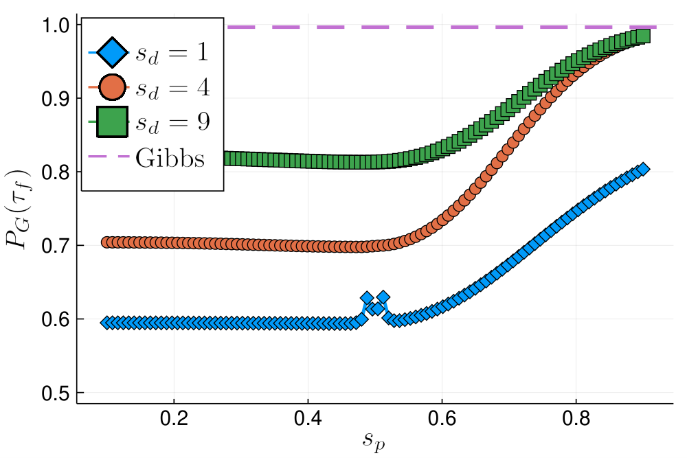
In addition, numerical results for a pausing schedule of the type shown in Fig. 2 are presented in Fig. 5. In these simulation we fixed the pausing duration $s_{d}$ and investigated the final success probability for different pausing positions $s_{p}$. Four primary observations arise from these results: (1) Increasing the total annealing time $t^{\prime}_{f}$ improves the final success probability. This is because we are neither close to the adiabatic limit (closed system) nor to thermal equilibrium (open system). (2) There is a peak (or more precisely, oscillations) in the success probability if we pause right around the minimum gap. However, for the parameters chosen here this is mainly a closed system effect which is suppressed in the open system setting (we show Sec. IV.4 below that the choice of the cutoff frequency matters a great deal). The oscillations can be understood as the interference pattern between two different paths leading to the final ground state Munoz-Bauza et al. 2019, because pausing splits the single region of diabatic evolution into two and effectively creates a Mach-Zehnder interferometer Oliver et al. 2005. (3) Pausing only helps if it happens after the minimum gap. This phenomenon can be explained by our analytic model presented in Sec. IV.3. (4) All the MEs still produce the same results in the presence of pausing, which suggests we may use the AME, since it has the simplest structure for pursuing analytical results.

We now present a theoretical analysis in support of the numerical results above, and to address the experimental findings in Ref. Marshall et al. 2019. Without loss of generality, we will assume $\theta(1)=\pi/2$ in the derivation. The proof also goes through for other boundary conditions. The first assumption we make is the localization of the geometric phase. To be more specific, we assume

$$\dot{\theta}\pqty{s}\approx 0\quad\forall s\notin\bqty{\mu_\theta-c\alpha_\theta, \mu_\theta+ c\alpha_\theta}$$

(32)

where $c$ is a dimensionless constant and $c\alpha_{\theta}$ measure the effective width of the Gaussian pulse. Later, we will take the limit $\alpha_{\theta}\to 0$. This condition holds for all the hard instances we consider in this work. In the small $\alpha_{\theta}$ limit, the Redfield Eq. (18) can be treated separately inside/outside the region $\bqty{\mu_\theta-c\alpha_\theta, \mu_\theta+ c\alpha_\theta}$. Within this Landau-Zener (LZ) region, the geometric phase dominates and all the other terms can be considered as a perturbation. With the detailed derivation given in Appendix E, we prove that, in the limit of weak coupling and small $\alpha_{\theta}$, the evolution across the LZ region can be approximated by a “diabatic pulse” unitary of the following form

$$U=\begin{pmatrix}\cos(\varphi)&-i\sin(\varphi)\\ -i\sin(\varphi)&\cos(\varphi)\end{pmatrix}\ ,$$

(33)

where

$$\varphi=\frac{\pi}{4}e^{-(t_{f}/t_{\mathrm{ad}})^{2}}\ ,\quad t_{\mathrm{ad}}=\frac{\sqrt{2}}{\alpha_{\theta}\int_{0}^{\mu_{\theta}}\Omega\pqty{s}\differential{s}}\ .$$

(34)

In the limit $\alpha_{\theta}\to 0$ the closed-system adiabatic time scale $t_{\mathrm{ad}}$ diverges. This is an approximation to real computational (small gap) problems where the adiabatic time scale is infinite for practical purposes.

Outside the LZ region, $\derivative{\theta}{\tau}\approx 0$ and hence the Hamiltonian (28) can be written as

$$H(\tau)=-\frac{t^{\prime}_{f}}{2}\Omega(\tau)Z+t^{\prime}_{f}\sum_{\alpha}g_{\alpha}S_{\alpha}\pqty{\tau}\otimes\mathcal{B}_{\alpha}+H_{\mathrm{B}}\ ,$$

(35)

We also assume the position of the pause is outside the LZ region:

$$s_{p}\notin\bqty{\mu_\theta^- , \mu_\theta^+},\qquad\mu_{\theta}^{\pm}\equiv\mu_{\theta}\pm c\alpha_{\theta}\ .$$

(36)

This is in accordance with the experimental protocol of Ref. Marshall et al. 2019, where pausing was found to be effective past the position of the avoided crossing, and is explained theoretically below in terms of the absence of a pausing effect before $s=\mu_{\theta}$.

Following Ref. Albash and Lidar 2015, the AME can be written as two fully decoupled parts, which simplifies the derivation compared to the other master equations considered above:

	$\displaystyle\dot{\rho}_{00}(\tau)$	$\displaystyle=-\dot{\rho}_{11}(\tau)=t^{\prime}_{f}\Gamma_{01}(\tau)\rho_{11}(\tau)-t^{\prime}_{f}\Gamma_{10}(\tau)\rho_{00}(\tau)$		(37a)
	$\displaystyle\dot{\rho}_{01}(\tau)$	$\displaystyle=-it^{\prime}_{f}\pqty{\omega_{01}(\tau)+\Sigma_{01}(\tau)}\rho_{01}(\tau)-\xi_{01}(\tau)\rho_{01}(\tau)$		(37b)

where

	$\displaystyle\omega_{01}(\tau)$	$\displaystyle=-\omega_{10}(\tau)=-\Omega(\tau)$		(38a)
	$\displaystyle\Gamma_{01}(\tau)$	$\displaystyle=\sum_{\alpha}\gamma_{\alpha}\pqty{\Omega(\tau)}\absolutevalue{S_\alpha^{01}(\tau)}^{2}=e^{\beta\Omega(\tau)}\Gamma_{10}(\tau)$		(38b)
	$\displaystyle\Sigma_{01}(\tau)$	$\displaystyle=-\Sigma_{10}(\tau)=\sum_{\alpha}\absolutevalue{S_\alpha^{01}}^{2}(\mathcal{S}(\omega_{01})-\mathcal{S}(\omega_{10}))$		(38c)
	$\displaystyle\xi_{01}\pqty{\tau}$	$\displaystyle=\frac{1}{2}\pqty{\Gamma_{01}+\Gamma_{10}}+\frac{1}{2}\sum_{\alpha}\gamma_{\alpha}\pqty{0}\absolutevalue{S^{00}_\alpha+ S^{11}_\alpha}$		(38d)

Our primary interest is in the ground state population [Eq. (37a)]. It can be rewritten as

	$\displaystyle\dot{\rho}_{00}(\tau)$	$\displaystyle=\Gamma(\tau)\bigg[1-\pqty{1+e^{-\beta\Omega(\tau)}}\rho_{00}(\tau)\bigg]$		(39a)
	$\displaystyle\Gamma(\tau)$	$\displaystyle\equiv t^{\prime}_{f}\Gamma_{01}(\tau)\ ,$		(39b)

where $\Gamma(\tau)$ is the dimensionless relaxation rate subject to pausing.²² 2 Recall our convention of denoting by $Q(s)$ the original quantity and by $Q(\tau)$ the corresponding paused quantity. In the case of $\Gamma(s)$ this includes the paused anneal time $t^{\prime}_{f}$, so in that sense it represents a mixed quantity. The off-diagonal elements of the density matrix decay exponentially with a rate determined by $\xi_{01}(\tau)$. As a consequence, if we start in the ground/thermal state of the initial Hamiltonian, right before the LZ region, the system density matrix will to an exponentially good approximation have only diagonal elements:

$$\rho(\mu_{\theta}^{-})=\matrixquantity(\lx@physics@matrix P(\mu^-_\theta) & 0 \\ 0 & 1-P(\mu^-_\theta)\endlx@physics@matrix)\ .$$

(40)

After crossing the LZ region, using Eq. (33) the state becomes

	$\displaystyle\rho(\mu_{\theta}^{+})$	$\displaystyle=\matrixquantity(\lx@physics@matrix P_\varphi& -i(P_0-P_1)\sin 2\varphi\\ i(P_0-P_1)\sin 2\varphi& 1-P_\varphi\endlx@physics@matrix)$		(41a)
	$\displaystyle P_{0}$	$\displaystyle=P(\mu_{\theta}^{-})=1-P_{1}$		(41b)
	$\displaystyle P_{\varphi}$	$\displaystyle=P_{0}\cos^{2}{\varphi}+P_{1}\sin^{2}{\varphi}\ .$		(41c)

Note that $P_{\varphi}$ is the ground state population right after the minimum gap is crossed. We can see from Eqs. (40) and (41) that pausing before $\mu_{\theta}$ has no effect on the final results. Therefore, in the following discussion, we will assume the pausing position is after the diabatic pulse: $s_{p}>\mu_{\theta}$. The solution of Eq. (39a) from $\mu^{+}_{\theta}$ to $\tau_{f}=1+s_{d}$ can be written as

	$\displaystyle\rho_{00}(\tau_{f})$	$\displaystyle=\exp[-\int_{\mu^{+}_{\theta}}^{\tau_{f}}\differential{\tau}\pqty{1+e^{-\beta\Omega(\tau)}}\Gamma(\tau)]$
		$\displaystyle\times\Bigg\{P_{\varphi}+\int_{\mu^{+}_{\theta}}^{\tau_{f}}\differential{\tau}\Gamma(\tau)$		(42a)
		$\displaystyle\times\exp[\int_{\mu^{+}_{\theta}}^{\tau}\differential{\tau'}\pqty{1+e^{-\beta\Omega(\tau')}}\Gamma(\tau^{\prime})]\Bigg\}$
		$\displaystyle=\mathcal{F}_{d}(\tau_{f},s_{p},s_{d})+\mathcal{F}_{g}(\tau_{f},s_{p},s_{d})\ ,$		(42b)

where

	$\displaystyle\mathcal{F}_{d}(\tau_{f},s_{p},s_{d})$	$\displaystyle=P_{\varphi}G(\mu^{+}_{\theta})$		(43a)
	$\displaystyle\mathcal{F}_{g}(\tau_{f},s_{p},s_{d})$	$\displaystyle=\int_{\mu^{+}_{\theta}}^{\tau_{f}}\differential{\tau}\Gamma(\tau)G(\tau)\ ,$		(43b)

and where

	$\displaystyle G(\tau)$	$\displaystyle=\exp\bigg(-\int_{\tau}^{\tau_f}\dd{\tau'}X(\tau')\bigg)$		(44a)
	$\displaystyle X(\tau)$	$\displaystyle=\bigg(1+e^{-\beta\Omega(\tau)}\bigg)\Gamma(\tau)\ .$		(44b)

Note that the functions $\Omega(\tau)$ and $\Gamma(\tau)$ have an implicit dependence on $s_{p}$ and $s_{d}$:

	$\displaystyle\Omega(\tau)$	$\displaystyle=\Omega(s(\tau))$		(45a)
	$\displaystyle\Gamma(\tau)$	$\displaystyle=(1+s_{d})t_{f}\sum_{\alpha}\gamma_{\alpha}[\Omega(s(\tau))]\absolutevalue{S_\alpha^{01}(s(\tau))}^{2},$		(45b)

where we combined Eqs. (38b) and  (39b). To achieve the maximum success probability, we need to solve the following optimization problem:

$$\argmax_{\Bqty{s_p, s_d}}\mathcal{F}_{d}(\tau_{f},s_{p},s_{d})+\mathcal{F}_{g}(\tau_{f},s_{p},s_{d})\ .$$

(46)

First, noticing that the quantities defined in Eqs. (44b), (45a), and (45b) can be functions of either $s$ (unpaused) or $\tau$ (paused), to avoid any ambiguity we henceforth use the notation $\bar{Q}(s)$ when the argument is $s$. For example, $\bar{\Gamma}(1)$ means $\Gamma(s=1)$ instead of $\Gamma(\tau=1)$. Note that this modifies our previous convention of denoting by $Q(s)$ the original quantity and by $Q(\tau)$ the corresponding paused quantity.

Then, we analyze the optimal pausing position $s_{p}^{*}$, for a given pausing duration $s_{d}$. We consider an Ohmic bath with different cutoff frequencies. This leads to different behaviors of the dimensionless relaxation rate $\bar{\Gamma}(s)$, from decreasing to non-monotonic to increasing, as illustrated in Fig. 6. Before proceeding, we emphasize that, as is clear from Eq. (45b), the monotonicity properties of $\bar{\Gamma}(s)$ depend on three different factors:

• •

  The gap of the projected TLS

• •

  The projected system-bath coupling operators [Eq. (24)]

• •

  The noise spectrum

In our examples, the first two are fixed by Eqs. (7) and (30) respectively. Thus, at a given temperature, what remains is only the noise spectrum, or more specifically the only tuning parameter for the monotonicity of $\bar{\Gamma}(s)$ is the Ohmic bath cutoff frequency $\omega_{c}$. The relationship between $\omega_{c}$ and the monotonicity of $\gamma(\omega)$ within the qubit frequency range, which is sufficient to determine the monotonicity of $\bar{\Gamma}(s)$, is not straightforward. Thus the values in Fig. 6 were chosen after numerical investigation. More generally, the first two factors above are of equal importance to the noise spectrum. For example, in the $16$-qubit problem of Ref. Dickson et al. 2013 with pure dephasing couplings, the strength of the projected system-bath coupling operators $\sum_{\alpha}\absolutevalue{S_\alpha^{01}(s(\tau))}^{2}$ plays a key role as well: it has a peak around the minimum gap region and decreases to almost zero afterwards.

The corresponding success probabilities as a function of pausing position obtained by numerically solving the AME and via the analytic expression (42) are shown in Fig. 7, and are in excellent agreement. There are two main observations:

• •

  An optimal pausing position exists in the middle of the anneal for the cases illustrated in Fig. 6 and Fig. 6 where $\bar{\Gamma}(s)$ is not monotonically increasing.

• •

  When $\bar{\Gamma}(s)$ is monotonically increasing after the minimum gap, it is always better to (trivially) pause near the end of anneal.

Guided by these numerical results, we next prove that a non-trivial optimal pausing position exists provided that the dimensionless relaxation rate given in Eq. (39b) (i.e., comparing the actual relaxation rate $\Gamma_{01}$ to the anneal time $t_{f}^{\prime}$) is monotonically decreasing, with respect to $s$, from the end of the avoided crossing to the end of the anneal.

In this section we prove the following theorem, which provides sufficient conditions for the existence of a non-trivial optimal pausing position, thus generalizing and formalizing the numerical evidence exhibited above.

We remark that the existence of a non-trivial optimal pausing point is possible under a substantially broader set of conditions than implied by Theorem 1, as is shown in our proof below. The Theorem states a simplified set of conditions for ease of presentation and interpretation. The reader who is not interested in the technical details of the proof may skip ahead to the conclusions in Sec. V.

The proof follows. Because $\partialderivative{\rho_{00}}{s_p}$ is a continuous function of $s_{p}$, a sufficient condition for Eq. (47) is

$$\partialderivative{\rho_{00}}{s_p}\Big|_{s_{p}=\mu^{+}_{\theta}}>0\quad\mathrm{and}\quad\partialderivative{\rho_{00}}{s_p}\Big|_{s_{p}=1}<0\ .$$

(48)

We thus divide the proof into two parts, one for each of these two inequalities.

References

- Kadowaki and Nishimori (1998) Tadashi Kadowaki and Hidetoshi Nishimori, “Quantum annealing in the transverse Ising model,” Phys. Rev. E 58, 5355 (1998).
- Das and Chakrabarti (2008) Arnab Das and Bikas K. Chakrabarti, “Colloquium: Quantum annealing and analog quantum computation,” Rev. Mod. Phys. 80, 1061–1081 (2008).
- Albash and Lidar (2018a) Tameem Albash and Daniel A. Lidar, “Adiabatic quantum computation,” Reviews of Modern Physics 90, 015002 (2018a).
- Hauke et al. (2020) Philipp Hauke, Helmut G Katzgraber, Wolfgang Lechner, Hidetoshi Nishimori, and William D Oliver, “Perspectives of quantum annealing: Methods and implementations,” Reports on Progress in Physics (2020).
- Rønnow et al. (2014) Troels F. Rønnow, Zhihui Wang, Joshua Job, Sergio Boixo, Sergei V. Isakov, David Wecker, John M. Martinis, Daniel A. Lidar, and Matthias Troyer, “Defining and detecting quantum speedup,” Science 345, 420–424 (2014).
- Denchev et al. (2016) Vasil S. Denchev, Sergio Boixo, Sergei V. Isakov, Nan Ding, Ryan Babbush, Vadim Smelyanskiy, John Martinis, and Hartmut Neven, “What is the computational value of finite-range tunneling?” Phys. Rev. X 6, 031015 (2016).
- King et al. (2018) Andrew D. King, Juan Carrasquilla, Jack Raymond, Isil Ozfidan, Evgeny Andriyash, Andrew Berkley, Mauricio Reis, Trevor Lanting, Richard Harris, Fabio Altomare, Kelly Boothby, Paul I. Bunyk, Colin Enderud, Alexandre Fréchette, Emile Hoskinson, Nicolas Ladizinsky, Travis Oh, Gabriel Poulin-Lamarre, Christopher Rich, Yuki Sato, Anatoly Yu. Smirnov, Loren J. Swenson, Mark H. Volkmann, Jed Whittaker, Jason Yao, Eric Ladizinsky, Mark W. Johnson, Jeremy Hilton, and Mohammad H. Amin, “Observation of topological phenomena in a programmable lattice of 1,800 qubits,” Nature 560, 456–460 (2018).
- Harris et al. (2018) R. Harris, Y. Sato, A. J. Berkley, M. Reis, F. Altomare, M. H. Amin, K. Boothby, P. Bunyk, C. Deng, C. Enderud, S. Huang, E. Hoskinson, M. W. Johnson, E. Ladizinsky, N. Ladizinsky, T. Lanting, R. Li, T. Medina, R. Molavi, R. Neufeld, T. Oh, I. Pavlov, I. Perminov, G. Poulin-Lamarre, C. Rich, A. Smirnov, L. Swenson, N. Tsai, M. Volkmann, J. Whittaker, and J. Yao, “Phase transitions in a programmable quantum spin glass simulator,” Science 361, 162 (2018).
- Albash and Lidar (2018b) Tameem Albash and Daniel A. Lidar, “Demonstration of a scaling advantage for a quantum annealer over simulated annealing,” Physical Review X 8, 031016– (2018b).
- Mandrà and Katzgraber (2018) Salvatore Mandrà and Helmut G Katzgraber, “A deceptive step towards quantum speedup detection,” Quantum Sci. Technol. 3, 04LT01 (2018).
- Mott et al. (2017) Alex Mott, Joshua Job, Jean-Roch Vlimant, Daniel Lidar, and Maria Spiropulu, “Solving a higgs optimization problem with quantum annealing for machine learning,” Nature 550, 375 EP – (2017).
- Pudenz et al. (2014) Kristen L Pudenz, Tameem Albash, and Daniel A Lidar, “Error-corrected quantum annealing with hundreds of qubits,” Nat. Commun. 5, 3243 (2014).
- Vinci et al. (2016) Walter Vinci, Tameem Albash, and Daniel A Lidar, “Nested quantum annealing correction,” npj Quant. Inf. 2, 16017 (2016).
- Vinci and Lidar (2018) Walter Vinci and Daniel A. Lidar, “Scalable effective-temperature reduction for quantum annealers via nested quantum annealing correction,” Physical Review A 97, 022308– (2018).
- Pearson et al. (2019) Adam Pearson, Anurag Mishra, Itay Hen, and Daniel A. Lidar, “Analog errors in quantum annealing: doom and hope,” npj Quantum Information 5, 107 (2019).
- Lanting et al. (2017) Trevor Lanting, Andrew D. King, Bram Evert, and Emile Hoskinson, “Experimental demonstration of perturbative anticrossing mitigation using nonuniform driver hamiltonians,” Physical Review A 96, 042322– (2017).
- Adame and McMahon (2020) Juan I. Adame and Peter L. McMahon, “Inhomogeneous driving in quantum annealers can result in orders-of-magnitude improvements in performance,” Quantum Science and Technology 5, 035011 (2020).
- Hsu (2019) Ting-Jui Hsu, “Quantum annealing with anneal path control: Application to 2-sat problems with known energy landscapes,” Communications in Computational Physics 26, 928–946 (2019).
- Yarkoni et al. (2019) Sheir Yarkoni, Hao Wang, Aske Plaat, and Thomas Bäck, “Boosting quantum annealing performance using evolution strategies for annealing offsets tuning,” in Quantum Technology and Optimization Problems, edited by Sebastian Feld and Claudia Linnhoff-Popien (Springer International Publishing, Cham, 2019) pp. 157–168.
- Roland and Cerf (2002) Jérémie Roland and Nicolas J. Cerf, “Quantum search by local adiabatic evolution,” Phys. Rev. A 65, 042308– (2002).
- Marshall et al. (2019) Jeffrey Marshall, Davide Venturelli, Itay Hen, and Eleanor G. Rieffel, “Power of Pausing: Advancing Understanding of Thermalization in Experimental Quantum Annealers,” Physical Review Applied 11, 044083 (2019).
- Inc. (2018) D-Wave Systems Inc., “The D-Wave 2000Q Quantum Computer Technology Overview,” (2018).
- Venturelli and Kondratyev (2019) Davide Venturelli and Alexei Kondratyev, “Reverse quantum annealing approach to portfolio optimization problems,” Quantum Machine Intelligence 1, 17–30 (2019).
- Vinci et al. (2019) Walter Vinci, Lorenzo Buffoni, Hossein Sadeghi, Amir Khoshaman, Evgeny Andriyash, and Mohammad H. Amin, “A path towards quantum advantage in training deep generative models with quantum annealers,” (2019), arXiv:1912.02119 [quant-ph] .
- Passarelli et al. (2019) G. Passarelli, V. Cataudella, and P. Lucignano, “Improving the quantum annealing of the ferromagnetic -spin model through pausing,” arXiv:1902.06788 (2019).
- Passarelli et al. (2020) Gianluca Passarelli, Ka-Wa Yip, Daniel A. Lidar, Hidetoshi Nishimori, and Procolo Lucignano, “Reverse quantum annealing of the $p$-spin model with relaxation,” Physical Review A 101, 022331 (2020), publisher: American Physical Society.
- Breuer and Petruccione (2002) H.-P. Breuer and F. Petruccione, The Theory of Open Quantum Systems (Oxford University Press, Oxford, 2002).
- Alicki and Lendi (2007) Robert Alicki and K. Lendi, Quantum Dynamical Semigroups and Applications (Springer Science & Business Media, 2007).
- Lidar (2019) Daniel A Lidar, “Lecture notes on the theory of open quantum systems,” arXiv preprint arXiv:1902.00967 (2019).
- Albash et al. (2012) Tameem Albash, Sergio Boixo, Daniel A Lidar, and Paolo Zanardi, “Quantum adiabatic markovian master equations,” New J. of Phys. 14, 123016 (2012).
- Albash and Lidar (2015) Tameem Albash and Daniel A. Lidar, “Decoherence in adiabatic quantum computation,” Physical Review A 91, 062320 (2015).
- Smirnov and Amin (2018) Anatoly Yu Smirnov and Mohammad H. Amin, “Theory of open quantum dynamics with hybrid noise,” New Journal of Physics 20, 103037 (2018).
- Dann et al. (2018) Roie Dann, Amikam Levy, and Ronnie Kosloff, “Time-dependent markovian quantum master equation,” Physical Review A 98, 052129– (2018).
- Mozgunov and Lidar (2020) Evgeny Mozgunov and Daniel Lidar, “Completely positive master equation for arbitrary driving and small level spacing,” Quantum 4, 227 (2020).
- Nathan and Rudner (2020) Frederik Nathan and Mark S. Rudner, “Universal lindblad equation for open quantum systems,” (2020), arXiv:2004.01469 [cond-mat.mes-hall] .
- Munoz-Bauza et al. (2019) Humberto Munoz-Bauza, Huo Chen, and Daniel Lidar, “A double-slit proposal for quantum annealing,” npj Quantum Information 5, 51 (2019).
- Vinci and Lidar (2017a) Walter Vinci and Daniel A. Lidar, “Non-stoquastic Hamiltonians in quantum annealing via geometric phases,” npj Quantum Information 3, 38 (2017a).
- Rezakhani et al. (2010) A. T. Rezakhani, D. F. Abasto, D. A. Lidar, and P. Zanardi, “Intrinsic geometry of quantum adiabatic evolution and quantum phase transitions,” Physical Review A 82, 012321 (2010).
- Jansen et al. (2007) Sabine Jansen, Mary-Beth Ruskai, and Ruedi Seiler, “Bounds for the adiabatic approximation with applications to quantum computation,” J. Math. Phys. 48, 102111 (2007).
- Vinci and Lidar (2017b) Walter Vinci and Daniel A. Lidar, “Non-stoquastic hamiltonians in quantum annealing via geometric phases,” npj Quant. Inf. 3, 38 (2017b).
- Bravyi et al. (2011) Sergey Bravyi, David P. DiVincenzo, and Daniel Loss, “Schrieffer–wolff transformation for quantum many-body systems,” Annals of Physics 326, 2793 – 2826 (2011).
- Consani and Warburton (2020) Gioele Consani and Paul A Warburton, “Effective hamiltonians for interacting superconducting qubits: local basis reduction and the schrieffer–wolff transformation,” New J. of Phys. 22, 053040 (2020).
- Lidar et al. (2009) Daniel A. Lidar, Ali T. Rezakhani, and Alioscia Hamma, “Adiabatic approximation with exponential accuracy for many-body systems and quantum computation,” Journal of Mathematical Physics 50, 102106 (2009).
- Dickson et al. (2013) N. G. Dickson, M. W. Johnson, M. H. Amin, R. Harris, F. Altomare, A. J. Berkley, P. Bunyk, J. Cai, E. M. Chapple, P. Chavez, F. Cioata, T. Cirip, P. deBuen, M. Drew-Brook, C. Enderud, S. Gildert, F. Hamze, J. P. Hilton, E. Hoskinson, K. Karimi, E. Ladizinsky, N. Ladizinsky, T. Lanting, T. Mahon, R. Neufeld, T. Oh, I. Perminov, C. Petroff, A. Przybysz, C. Rich, P. Spear, A. Tcaciuc, M. C. Thom, E. Tolkacheva, S. Uchaikin, J. Wang, A. B. Wilson, Z. Merali, and G. Rose, “Thermally assisted quantum annealing of a 16-qubit problem,” Nature Communications 4, 1903 (2013).
- Yan et al. (2016) Fei Yan, Simon Gustavsson, Archana Kamal, Jeffrey Birenbaum, Adam P Sears, David Hover, Ted J. Gudmundsen, Danna Rosenberg, Gabriel Samach, S Weber, Jonilyn L. Yoder, Terry P. Orlando, John Clarke, Andrew J. Kerman, and William D. Oliver, “The flux qubit revisited to enhance coherence and reproducibility,” Nature Communications 7, 12964 EP – (2016).
- Quintana et al. (2017) C. M. Quintana, Yu Chen, D. Sank, A. G. Petukhov, T. C. White, Dvir Kafri, B. Chiaro, A. Megrant, R. Barends, B. Campbell, Z. Chen, A. Dunsworth, A. G. Fowler, R. Graff, E. Jeffrey, J. Kelly, E. Lucero, J. Y. Mutus, M. Neeley, C. Neill, P. J. J. O’Malley, P. Roushan, A. Shabani, V. N. Smelyanskiy, A. Vainsencher, J. Wenner, H. Neven, and John M. Martinis, “Observation of classical-quantum crossover of flux noise and its paramagnetic temperature dependence,” Physical Review Letters 118, 057702– (2017).
- Novikov et al. (2018) S. Novikov, R. Hinkey, S. Disseler, J. I. Basham, T. Albash, A. Risinger, D. Ferguson, D. A. Lidar, and K. M. Zick, “Exploring more-coherent quantum annealing,” in 2018 IEEE International Conference on Rebooting Computing (ICRC) (2018) pp. 1–7.
- Khezri et al. (2020) Mostafa Khezri, Jeffrey A. Grover, James I. Basham, Steven M. Disseler, Huo Chen, Sergey Novikov, Kenneth M. Zick, and Daniel A. Lidar, “Anneal-path correction in flux qubits,” (2020), arXiv:2002.11217 [quant-ph] .
- Oliver et al. (2005) William D. Oliver, Yang Yu, Janice C. Lee, Karl K. Berggren, Leonid S. Levitov, and Terry P. Orlando, “Mach-zehnder interferometry in a strongly driven superconducting qubit,” Science 310, 1653 (2005).
- (50) Eric W. Weisstein, “Lambert W-Function.” From MathWorld–A Wolfram Web Resource .
- Altshuler et al. (2010) Boris Altshuler, Hari Krovi, and Jérémie Roland, “Anderson localization makes adiabatic quantum optimization fail,” Proceedings of the National Academy of Sciences 107, 12446–12450 (2010).
- Izquierdo et al. (2020) Zoe Gonzalez Izquierdo, Shon Grabbe, Stuart Hadfield, Jeffrey Marshall, Zhihui Wang, and Eleanor Rieffel, “Ferromagnetically shifting the power of pausing,” arXiv:2006.08526 (2020).
- Shin et al. (2014) Seung Woo Shin, Graeme Smith, John A. Smolin, and Umesh Vazirani, “How “quantum” is the D-Wave machine?” arXiv:1401.7087 (2014).
- Marshall and Albash (2020) Jeffrey Marshall and Tameem Albash, (2020), private communication.
- Bezanson et al. (2017) J. Bezanson, A. Edelman, S. Karpinski, and V. Shah, “Julia: A Fresh Approach to Numerical Computing,” SIAM Review 59, 65–98 (2017).
- Rackauckas and Nie (2017) Christopher Rackauckas and Qing Nie, “DifferentialEquations.jl – A Performant and Feature-Rich Ecosystem for Solving Differential Equations in Julia,” Journal of Open Research Software 5 (2017), 10.5334/jors.151.
- Andrew and Tan (1998) Alan L. Andrew and Roger C. E. Tan, “Computation of Derivatives of Repeated Eigenvalues and the Corresponding Eigenvectors of Symmetric Matrix Pencils,” SIAM Journal on Matrix Analysis and Applications 20, 78–100 (1998).