GPU-accelerated massive black hole binary parameter estimation with LISAPreprint: APS/123-QED
Abstract
The Laser Interferometer Space Antenna (LISA) is slated for launch in the early 2030s. A main target of the mission is massive black hole binaries that have an expected detection rate of yr-1. We present a parameter estimation analysis for a variety of massive black hole binaries. This analysis is performed with a graphics processing unit (GPU) implementation comprising the PhenomHM waveform with higher-order harmonic modes and aligned spins; a fast frequency-domain LISA detector response function; and a GPU-native likelihood computation. The computational performance achieved with the GPU is shown to be 500 times greater than with a similar CPU implementation, which allows us to analyze full noise-infused injections at a realistic Fourier bin width for the LISA mission in a tractable and efficient amount of time. With these fast likelihood computations, we study the effect of adding aligned spins to an analysis with higher-order modes by testing different configurations of spins in the injection, as well as the effect of varied and fixed spins during sampling. Within these tests, we examine three different binaries with varying mass ratios, redshifts, sky locations, and detector-frame total masses ranging over three orders of magnitude. We discuss varied correlations between the total masses and mass ratios; unique spin posteriors for the larger mass binaries; and the constraints on parameters when fixing spins during sampling, allowing us to compare to previous analyses that did not include aligned spins.
I Introduction
The Laser Interferometer Space Antenna (LISA), an ESA-led mission, is officially slated for launch in the early 2030s (Amaro-Seoane et al 2017). LISA will add the mHz regime of the gravitational wave spectrum to the high-frequency observations by the LIGO–Virgo–KAGRA network (The LIGO Scientific Collaboration and the Virgo Collaboration 2018; LVK Collaboration 2018). A primary source of interest for LISA is the inspiral and merger of massive black hole (MBH) binaries. Recent work has shown that LISA is expected to detect – MBH binaries per year (Klein et al. 2016; Berti et al. 2016; Salcido et al. 2016; Katz et al. 2019; Bonetti et al. 2019). These sources are expected to occur at high signal-to-noise ratios (SNRs) of – out to high redshifts (–) (eLISA Consortium 2013; Barausse et al. 2015; Amaro-Seoane et al 2017). LISA will be sensitive to binaries of – if they exist (Amaro-Seoane et al 2017; Klein et al. 2016; Katz and Larson 2019).
The high SNR of MBH signals will help astronomers understand the formation and evolution of these objects over cosmic time (eLISA Consortium 2013; Barausse et al. 2015; Amaro-Seoane et al 2017). Theories of MBH formation channels usually fall into three categories: high-mass seeds of – from pre-galactic halo collapse at – (Loeb and Rasio 1994; Begelman et al. 2006; Latif et al. 2013; Habouzit et al. 2016; Ardaneh et al. 2018; Dunn et al. 2018); intermediate seeds of – from runaway cluster collapse at – (Omukai et al. 2008; Devecchi and Volonteri 2009; Davies et al. 2011; Katz et al. 2015); and smaller seeds of from the collapse of Population III stars at – (Haiman et al. 2000; Fryer et al. 2001; Heger et al. 2003; Volonteri et al. 2003; Tanaka and Haiman 2009; Alvarez et al. 2009). The loud signals from MBH binaries can also be used for tests of fundamental physics and independent measurements of cosmological parameters (Petiteau et al. 2011; Gair et al. 2013; Barausse et al. 2015). In addition, determining MBH binary information like the sky location and masses is crucial in the search for electromagnetic counterparts. This search requires efficient and reliable measurement of such parameters prior to the actual merger of the two MBHs. With electromagnetic counterparts to MBH mergers, further questions about cosmology can be answered (Schutz 1986; Holz and Hughes 2005), as well as questions related to accretion processes and active galactic nuclei (Armitage and Natarajan 2002; Burke-Spolaor 2013; Bogdanović 2015; Dal Canton et al. 2019).
Traditionally, Bayesian inference techniques have been suggested for MBH binary searches and statistical analysis (Cornish and Porter 2006; Cornish and Porter 2007; Porter and Carré 2014; Porter and Cornish 2015; Marsat et al. 2020, e.g.). Prior to the use of modern Bayesian sampling techniques (Christensen and Meyer 1998), the Fisher information matrix (FIM) approach was an accepted method for determining the uncertainties of measurable quantities; however, it has been shown that FIM analyses do not encompass the necessary information to make strong statements about parameter estimation with MBH binaries (Porter and Cornish 2008; Vallisneri 2008; Porter and Cornish 2015, e.g.). Similarly, it is important to include more advanced waveform models that better describe the physics of binary black hole coalescence. Aspects like higher-order harmonic modes help to further constrain parameters, remove systematic bias, and to further understand the characteristics of actual data analysis when the LISA mission is launched. Any difference between the waveform models used to create our templates and the true signals that will be observed by LISA will create systematic error (Cutler and Vallisneri 2007). However, in this work, we will inject the same waveform model as the model used for the templates, therefore bypassing this issue.
In this paper, we examine MBH parameter estimation under the new LISA sensitivity (Amaro-Seoane et al 2017; Team 2018) by using modern, computationally enhanced inspiral–merger–ringdown waveforms that include higher-order harmonics and aligned spins. A variety of LISA-related parameter estimation studies have previously been performed for MBH binaries. The work in (Cutler and Flanagan 1994; Vecchio 2004; Arun 2006; Berti et al. 2005; Lang and Hughes 2006) addressed this problem with FIM estimates, the low-frequency approximation to the LISA response function, and inspiral-only Newtonian waveforms. The Mock LISA Data Challenges (Babak et al. 2010) expanded on these studies by developing MCMC methods towards the source search problem. Improving upon these analyses further, Bayesian inference techniques were developed in (Brown et al. 2007; Cornish and Porter 2006; Crowder et al. 2006; Wickham et al. 2006; Röver et al. 2007; Feroz et al. 2009; Gair and Porter 2009; Petiteau et al. 2009; Porter and Carré 2014; Porter and Cornish 2015). However, these works still employed inspiral-only waveforms.
The effect of using higher-order harmonic corrections in studies of MBH binaries was examined in (Arun et al. 2007; Trias and Sintes 2008; Porter and Cornish 2008; McWilliams et al. 2010a). Analyses of waveforms including merger and ringdown were examined with the FIM method in (McWilliams et al. 2010a; Thorpe et al. 2009; McWilliams et al. 2010b; McWilliams et al. 2011) and with a Bayesian approach in Babak et al. 2008. Babak et al. 2014 used the FIM method to analyse parameter constraints with a variety of LISA designs. This study used inspiral waveforms with a reweighting scheme to account for the contribution of the merger and ringdown. Baibhav et al. 2020 recently studied the ability to constrain parameters using only ringdown signals with higher-order harmonics. This study used the FIM method, no noise, and an analytical description of the ringdown.
Marsat et al. 2020 was the first study to use a full Bayesian analysis on waveforms that include inspiral, merger, and ringdown. This analysis examined Schwarzschild MBHs, and featured a new prescription for the LISA response function by Marsat and Baker 2018. They used MCMC methods to characterize only extrinsic parameters, by employing a noiseless injection that included higher-order modes. In this work, we extend the findings of Marsat et al. 2020 to include MBH signals with aligned spins, injected into a data stream that includes realistic LISA noise. We also analyze the full parameter space of MBH binaries, including both intrinsic and extrinsic quantities.
Many of the analyses mentioned above were performed using the original LISA sensitivity curve (Larson et al. 2000). The changes to the LISA sensitivity curve in the most recent ESA-approved proposal (Amaro-Seoane et al 2017) are expected to severely affect our ability to measure and characterize MBH binaries (Katz and Larson 2019). First, the SNR for a general MBH binary source will be slightly lower due to higher noise at the low-frequency end and a smaller arm length (2.5 Gm versus 5 Gm). Additionally, it can be shown we will observe MBH mergers for less time with the new LISA sensitivity curve (Amaro-Seoane et al 2017), compared to previous predictions under the classic LISA sensitivity curve (Larson et al. 2000). For some mergers, we will observe their signal for only a few days, instead of the originally estimated weeks or months.
Figure 1 shows the SNR over time for the binaries (described in Section IV) that are studied in this work. For this plot, we employ a simplified calculation of the sky-location-, polarization-, and inclination-averaged SNR for the mode, with the gwsnrcalc package (Katz and Larson 2019) that uses PhenomD (Husa et al. 2016; Khan et al. 2016), Equation 3, and an averaging factor of 16/5 (Cornish and Robson 2018). It can be seen that, for the binaries tested, we will observe them for days, whereas with the classic LISA sensitivity, we can observe them for months. As a result of this difference in observation time, sky localization is not expected to be satisfactory until close to or after the merger. Early, accurate notifications for astronomers are critical for detecting electromagnetic counterparts to MBH binary mergers. Developing low-latency algorithms and computational infrastructure improvements for faster analysis is essential for this process.
In Section II, we discuss Bayesian inference in the context of MBH signals and the LISA mission. This includes our GPU-accelerated implementations of the waveform, LISA response, and the Bayesian likelihood, which prove to be very beneficial when examining a more complete version of the LISA analysis problem that includes a full noise realization. We detail our sampling methods in Section III. In Section IV, we discuss the sample data sets we analyzed, our ability to infer the proper parameters, and information gained about LISA parameter estimation through running our tests. For our analysis, we use units with .
II Bayesian Inference with Gravitational Waves from Massive Black Holes
In the field of gravitational waves, the data stream, , consists of a possible signal, , as well as noise, (. In our theoretical study, we will generate the data set by injecting a signal both with and without noise. We will then estimate the parameters of the source in the fabricated data set using Bayesian inference techniques. Bayesian inference methods are based on Bayes rule given by,
| (1) |
where and represent the underlying model and model parameters, respectively. The probability on the left-hand side of this equation is the posterior probability, which is the main value we are concerned with determining. The posterior probability represents the probability for the model parameters given the observed data and assumed model. In our study, the parameter set exists in , where is the number of dimensions we test. The parameter set we examine is {}, which represents, in order, the total mass, mass ratio, dimensionless spin of the larger black hole, dimensionless spin of the smaller black hole, luminosity distance, reference phase, inclination, ecliptic longitude, ecliptic latitude, polarization angle, and reference time. As discussed in Section II.1, the spins of the two MBHs are assumed to be aligned to the orbital angular momentum vector, therefore, reducing our parameter space from to since the spins are represented only as magnitudes without vector angles. For our underlying model, , we will only examine one waveform model. Therefore, we will drop the throughout the rest of this paper.
The prior probability, , is based on prior knowledge of the potential true parameters representing the injection. For our analysis, we assume limited prior knowledge by employing uniform priors across our parameters throughout an encompassing volume. Information on the priors used can be found in Table 1.
| Parameter | Lower Bound | Upper Bound |
| 0.05 | 1.0 | |
| -0.99 | 0.99 | |
| -0.99 | 0.99 | |
| 0.0 | ||
| -1.0 | 1.0 | |
| 0.0 | ||
| -1.0 | 1.0 | |
| 0.0 | ||
The key element of Bayesian analysis involves the calculation of the Likelihood, . In the case of gravitational waves, is the probability for the observed data given a set of parameters and assumed underlying model. The negative log of the Likelihood (NLL) is given by,
| (2) |
where is the template waveform, is the data stream, and is the noise-weighted inner product of the Fourier transforms of two time series and . The Fourier transform of a(t) is represented as . The inner product is given by,
| (3) |
where is the one-sided power spectral density (PSD) of the noise. The template, , is built from the same model as the injected signal, ; however, we use to represent the true signal to avoid confusion. The optimal SNR attainable by a template is . Here, we treat as constant over the observation duration for simplicity. In reality, the noise is expected to vary slowly with time allowing for noise estimation on the order of week when the instantaneous gravitational wave amplitude is well below the noise. For reference, the error in noise estimation is a second-order effect on the statistics illuminated by parameter estimation (Edwards et al. 2015; Littenberg and Cornish 2015; Biscoveanu et al. 2020).
The denominator on the right-hand side of Equation 1 is referred to as the evidence, . The evidence is the marginalization of the likelihood over the parameter space,
| (4) |
The evidence, generally, helps estimate the fidelity of a model and to compare models with one another. Computing the evidence directly in the gravitational wave setting is intractable. However, in the Markov Chain Monte Carlo (MCMC) analysis described in Section III, the evidence enters only as a multiplicative constant. Therefore, we do not need to compute the evidence for our chosen analysis method. However, as we will describe in Section III, we employ a parallel tempering version of MCMC. Within the parallel tempering method, the evidence can be estimated using techniques such as Thermodynamic Integration (Goggans and Chi 2004; Lartillot and Philippe 2006) or Stepping-Stone Sampling (Maturana-Russel et al. 2019).
To determine the signals and templates, we use the frequency domain waveform model for binary black hole coalescence PhenomHM (Husa et al. 2016; Khan et al. 2016; London et al. 2018). We refer the interested reader to Kalaghatgi et al. 2019 for questions related to systematic errors in this waveform model. PhenomHM includes aligned spins, higher order spherical harmonic modes, and all three stages of binary black hole coalescence: inspiral, merger, and ringdown. This is the first study of its kind for LISA MBH analysis to include all three of these properties simultaneously. In this work, we analyze the parameter estimation portion of LISA data analysis. We do not perform the initial search for the source; instead, we assume a source has already been identified in the data stream. Additionally, we also ignore any effects from the superposition of signals from other sources simultaneously evolving in the LISA data.
The set of inputs to the waveform model are {}. In our implementation of the waveform, we receive the amplitude, A, and the phase, , of each input spherical harmonic mode , given by,
| (5) |
There are six spherical harmonic modes within the PhenomHM model: . The (2,2) mode is the dominant mode. The other modes are referred to as higher harmonics or higher modes. An example of the PhenomHM amplitudes for each harmonic mode is shown in the left plot of Figure 2.
The frequency bounds of the waveform are determined from the merger time of the signal. We choose a coalescence time, yr into the LISA observing window. In our methodology, for our true signal we set . is on the order of a year and defines a temporal marker around which we analyze our signal. represents the fine tuning of to the actual coalescence time; therefore, is on the scale of seconds to months. represents the time at which the waveform reaches for the (2,2) mode, which is determined internally within PhenomHM to be the frequency at which reaches a maximum (see (London et al. 2018) and (Khan et al. 2016) for more information). Due to the complicated nature of the time-frequency correspondence across multiple higher order modes, we determine the time evolution of the system using the derivative of the phase and its relation to given by,
| (6) |
We make a cut in frequency when falls below zero for each individual mode, indicating the initial point of the waveform in the detector when LISA initially begins taking data.
We then apply the transfer function projecting the waveform onto the detector. The LISA response involves a complex time- and frequency-dependent transfer function (Cutler and Flanagan 1994; Larson et al. 2000; Cornish and Rubbo 2003; Marsat and Baker 2018). We apply the fast Fourier domain response from Marsat and Baker 2018. Therefore, the signal in the LISA detector is represented by,
| (7) |
where is the response transfer function and {A, E, T} are the time-delay interferometry (TDI) channel indicators. TDI is necessary for LISA to suppress laser noise (Tinto and Armstrong 1999; Armstrong et al. 1999; Estabrook et al. 2000; Dhurandhar et al. 2002; Tinto and Dhurandhar 2005). The A, E, and T channels are transformations of the original X, Y, and Z Michelson TDI observables (Vallisneri 2005) given by,
| (8) | ||||
| (9) | ||||
| (10) |
Employing channels A, E, and T, we assume the noise in each channel is uncorrelated, giving a diagonalized noise matrix (Tinto and Dhurandhar 2014; Muratore et al. 2020). is determined using the extrinsic parameters, {} ( is factored into ); the time-frequency correspondance of the waveform; and the orbital and rotational properties of the LISA constellation. {} are used in the solar system baricenter (SSB) frame when determining ; however, during MCMC runs, these parameters are sampled in the LISA frame and then converted to the SSB frame before waveform generation. For details on the construction and methodology of , please see Marsat and Baker 2018 and Marsat et al. 2020. An example of the PhenomHM waveform amplitudes fed through the response function can be seen in the right plot in Figure 2.
With the waveforms in each TDI channel, we need the PSD of the noise in each channel, . We use the tdi package from the LISA Data Challenges Working Group software collection to generate our PSD in each channel. Within the tdi package, we analyze the “SciRDv1” model (Team 2018) for the PSD with a contribution from the Galactic background noise predicted for 1 year into LISA observation. This Galactic background noise is described in Babak et al. 2017. Figure 2 shows the PSD1/2 shown in the left plot, which includes the contribution from the Galactic background. In the right side plot of the same figure, the PSD1/2 is shown in the TDI A channel. In Equation 2, the inner product is really the sum of the inner products over all three channels:
| (11) |
We analyze both data sets with noise () and without noise (). However, the weighting factor in Equation 3 applies in both cases as it defines the SNR. When we are assuming standard LISA noise assumptions while analyzing the unlikely scenario the noise assumes its average value of zero. When we do generate noise as part of the data, we generate it in the frequency domain given by,
| (12) |
where represents a normal distribution with mean and standard deviation , and is the Fourier bin width equivalent to 1/. It is then assigned a random phase from 0 to based on a uniform distribution.
With the tools to calculate the likelihood, we will now discuss acceleration of the process using graphics processing units (GPUs).
II.1 GPU Accelerated Waveforms and Likelihoods
A GPU is a special piece of hardware designed for parallel computation. They were originally designed for graphics cards related to video games and other video-related areas; however, as of the mid-2000s, it was realized these units could be re-purposed for general computational and academic use under the description: general purpose computing on graphics processing units (GPGPU). Here, we implement our PhenomHM waveforms, LISA response calculation, and likelihood computation in NVIDIA’s proprietary GPU programming language CUDA (Nickolls et al. 2008). GPUs have been used in gravitational wave analysis in Talbot et al. 2019, where they have implemented PhenomPv2 (Hannam et al. 2014), a waveform for the (2,2) mode with precessing spins, directly in CUDA for the LIGO Algorithmic Library (LIGO Scientific Collaboration 2018, LAL;). We take a different approach to our waveform implementation. Additionally, we have the first GPU implementation for the LISA fast response from Marsat and Baker 2018. We will introduce our implementation and then provide some timing results compared to a similar CPU-based program. For our timing tests, we used a Tesla V100 GPU and a Xeon Gold 6132 2.60 GHz CPU.
The main goal of our implementation is to perform as much of the computation as is feasible and beneficial on the GPU, while reducing the number and size of necessary memory transfers. Before beginning sampling where we will calculate the Likelihood times, we perform the aspects of this computation that only need to be completed once. These include inputting our data stream, , PSD information, and transferring this information to the GPU. Following these initial steps, we begin the calculation process that occurs each time we call the Likelihood function.
The first part of the PhenomHM creation process, which involves determining fitting constants from input parameters, is implemented in the C++ programming language. Structures containing these constants are then copied to the GPU. From here, the actual waveform creation from these fitting constants is implemented in parallel across the GPU because each frequency point is independent of one another. With the waveform constants, the amplitude and phase are generated and stored on the GPU. We then calculate using Equation 6. is input into the response function with the extrinsic parameters. is calculated on the GPU and stored on the GPU for each frequency point. At this stage, , , and are represented as smooth functions with frequency points. In LISA analysis, the data streams can be represented by upwards of points depending on the sampling frequency and duration of observation. Therefore, to maintain speed in data analysis, these smooth functions describing the waveform and detector response are interpolated to the resolution desired. We designed a cubic spline interpolation algorithm, for each of these smooth functions, based on the tridiagonal nature of the cubic spline coefficient solution in the Scipy library (Jones et al.) and the sparse matrix computational tools included in the cuSparse library provided by NVIDIA (cuS). This allowed us to avoid memory transfers necessary to perform spline interpolation on the CPU. The final step of waveform creation is to interpolate all input smooth functions to create the signal in each TDI channel. In this step, we weight by the PSD. With the waveform calculated and on the GPU, we use the cuBLAS library (cuB) to compute complex dot products for the discretized inner product in Equation 2 and Equation 11. The likelihood is then calculated and returned to the sampling program.
For ease of usage, our program is wrapped into Python using Cython (Behnel et al. 2011). This allows us to run python sampling packages using our GPU-accelerated likelihood calculation. Cython generally does not interface with the CUDA-based compiler nvcc. However, we wrote a special wrapping for it based on McGibbon and Zhao.
Speed comparisons are shown in Figure 3. Three configurations are shown: 1 CPU; 1 CPU and 1 GPU (host and device); and 28 CPUS and 2 GPUs. The last configuration vectorizes the computation over an array of sources. Therefore, these timings are run in vectorized form and then divided by the number of binaries in the array. As the points in the waveform increase, the difference between the CPU and GPU grows. The time of GPU evaluations barely increases until points. Above this number, the GPU is saturated, running a high percentage of its available threads constantly.
This increase in speed allows us to perform our analysis in a unique way. Traditionally, in a zero-noise representation, each spherical harmonic mode is treated separately in the Likelihood computation (see Marsat et al. 2020 for an example of this method). CPUs are not fast enough to efficiently compute the number of points necessary for combining all modes at a high enough resolution to preserve the fine structure created during the mixing of the higher modes. However, this is a balancing act because as more modes are added, the cross-terms between modes in Equation 2 become extensive and prohibitive. With GPUs, the time for the calculation allows us to forgo this question and produce templates at a high enough resolution to combine the modes into a one-dimensional data stream. This prevents the calculation of cross-terms and allows us to caclulate one inner product per TDI channel. Additionally, CPU speed prohibits the timely evaluation of Likelihoods with noise infused in the injection. With yrs, in the Fourier transform is Hz, leading to data streams with points. Similarly, for a typical source expected for LISA with , the waveform must be calculated at points. For lower masses, this is even larger. Therefore, CPUs have large difficulty performing this calculation with noise involved without including approximations and other tricks to speed up the calculation. The GPUs, on the other hand, facilitate the use of the brute-force calculation, without approximations. In the future, we may test different approximations in our GPU implementation to gain even more performance.
III Sampling Methods
There have been a large variety of methods developed to illuminate the posterior distribution, , as well as to calculate the evidence, . Two commonly used methods include Nested Sampling (Skilling 2004; Skilling 2006) and Markov Chain Monte Carlo (MCMC) methods, for which the most commonly used type is the Metropolis-Hastings (M-H) algorithm (Metropolis and Ulam 1949; Metropolis et al. 1953; Hastings 1970). Nested sampling is generally used to estimate the evidence, , by effectively performing a numerical integration across the prior volume. MCMC, on the other hand, is used to sample directly from the posterior to produce marginalized posterior distributions across the parameters tested. In this work, we will employ only MCMC techniques to illuminate our posterior distributions for the injected signals we examine. However, we have tested our accelerated likelihood with Nested Sampling techniques and have confirmed its possible usage as a search method. This will be included in future work. For actual sampling, we use variants of the typical MCMC techniques. Below, we will give a brief description of the algorithms used, but refer the interested reader to the cited papers for further details on the specific algorithms and their implementations.
III.1 Markov Chain Monte Carlo
The implementation we use for MCMC methods is based on the Python packages emcee (Foreman-Mackey et al. 2013) and ptemcee (Vousden et al. 2016). Please see their release papers and documentation for details on specific constructions. The most popular form of MCMC is the M-H algorithm. Starting with a position at step , a new position, , is sampled from a transition distribution . This new point is then accepted with a probability given by,
| (13) |
A usual choise for is a multivariate Gaussian distribution centered around . This procedure has strong dependence on tuning the distribution for (the covariance matrix for a multivariate Gaussian) with order tuning parameters. Additionally, the M-H algorithm can be slow to convergence if tuning is not optimal (Foreman-Mackey et al. 2013).
Goodman and Weare 2010 proposed a different method for MCMC sampling that significantly outperforms M-H in many situations. Specifically, this means the autocorrelation time (see Section III.3) of the MCMC chains is much less, indicating less Likelihood evaluations per independent sample. This method is refered to as Affine Invariant MCMC (AIMCMC). In AIMCMC, the sampler evolves an ensemble of walkers . The algorithm proposes a new position for the th walker based on the other walkers in the ensemble (). First, a walker is chosen at random from , represented by . Then, a new position is proposed given by,
| (14) |
where Y is a random variable distributed according to the probability density , given by (Goodman and Weare 2010),
| (15) |
where is a tuning parameter that Goodman and Weare 2010 set to 2. This proposal is referred to as the “stretch” proposal. The proposed point will be accepted according to the probability, , given by,
| (16) |
III.2 Parallel Tempering
In order to efficiently explore the entire prior range, we employ parallel tempering (Swendsen and Wang 1986; Earl and Deem 2005). Specifically, we use the implementation from Vousden et al. 2016 and its associated Python package, ptemcee. Here, we present the main aspects of parallel tempering, but we refer the interested reader to Vousden et al. 2016, and sources within, for more detailed information.
In parallel tempering, the Likelihood in Equation 1 becomes , where is the temperature of a given chain. Groups of MCMC walkers are assigned to a specific temperature arranged in a ladder with rungs: . is 1, indicating chains assigned to that temperature represent the target distribution. As temperature increases, the tempered distribution becomes more and more representative of the prior distribution rather than the target distribution.
Each chain explores its tempered distribution using the AIMCMC algorithm with stretch proposals. At specified intervals, chains can swap temperatures according to an M-H acceptance criterion given by (Vousden et al. 2016),
| (17) |
where is the inverse temperature of chain . The form of Equation 17 indicates that temperature swaps usually occur between chains at adjacent rungs in the temperature ladder. We set the max temperature to infinity per the ptemcee documentation. Setting the max temperature to infinity means the highest temperature chain is exclusively exploring the prior distribution. We also use the adaptive tempering option. For more details on the adaptive method, please see the original paper.
The parallel tempered run for each binary was performed under the same settings. With the highest temperature, , set to , the remaining temperatures are geometrically spaced set by ptemcee defaults using log-spacing between 1 and (2.04807 is chosen based on the dimensionality of the parameter space). We set the scale factor () in Equation 15 to 1.15. We found the default setting of 2 was showing an undesirably small acceptance fraction for proposed jumps. We run a burn in of steps for each run. In Marsat et al. 2020, it is shown that we can generally expect 8 sky location posterior modes in the LISA reference frame (as opposed to the SSB reference frame). The longitudinal modes are located at values separated by from the true longitude value. Each of these four values has an associated latitudinal value that is either above or below the LISA orbital plane at . We use this information to ensure faster convergence in our sampler by placing 4 walkers in each temperature group at each of the 8 sky modes. It is clear from our analysis that our burn in phase allows the walkers to spread out accordingly away from modes that are not likely. We also verified that if we start all the walkers on the correct mode, the walkers spread out and locate the other modes if there is posterior weight there thanks to the tempering technique.
III.3 MCMC Autocorrelation Time
The posterior samples generated in an MCMC analysis are not independent. Therefore, we estimate the autocorrelation within a chain, referred to as the autocorrelation time, , following Sokal 1997 and Foreman-Mackey 2018. With multiple chains sampled based on methods described above, we work to estimate the mean, , and variance, , of the posterior distribution. The sampling variance, , on these estimators is given by,
| (18) |
Therefore, the effective sample size (ESS) is N/, representing the number of samples necessary to reduce the variance in the estimator to an acceptable value.
We estimate the autocorrelation time with the estimator for the normalized autocorrelation function, . This is based on the chain generated for each walker, , and is given by,
| (19) |
with
| (20) |
The mean of the chain, , is given by,
| (21) |
The integrated autocorrelation estimator is given by,
| (22) |
where . Sokal 1997 suggests using the smallest value of that satisfies . With the multiple chains generated with emcee, the variance in the estimator is reduced. Therefore, according to Foreman-Mackey 2018, this procedure is satisfactory for chains longer than . We thin the chains by this value before plotting posteriors to achieve a set of effectively independent samples.
IV Results and Discussion
1 This binary was injected without a noise realization.
2 and are fixed during sampling.
| Binary | SNR | |||||||||||
| - | () | - | - | Gpc | - | - | - | - | - | sec | - | |
| 1 | 1/3 | 0.0 | 0.0 | 36.59 | 2.14 | 1.05 | -0.024 | 0.62 | 2.03 | 50.25 | 588 | |
| 21 | 1/3 | 0.0 | 0.0 | 36.59 | 2.14 | 1.05 | -0.024 | 0.62 | 2.03 | 50.25 | 588 | |
| 32 | 1/3 | 0.0 | 0.0 | 36.59 | 2.14 | 1.05 | -0.024 | 0.62 | 2.03 | 50.25 | 588 | |
| 4 | 1/3 | 0.85 | 0.88 | 36.59 | 2.14 | 1.05 | -0.024 | 0.62 | 2.03 | 50.25 | 878 | |
| 5 | 1/3 | -0.83 | -0.89 | 36.59 | 2.14 | 1.05 | -0.024 | 0.62 | 2.03 | 50.25 | 473 | |
| 6 | 1/5 | 0.0 | 0.0 | 15.93 | 3.10 | 1.34 | 4.21 | -0.73 | 0.14 | 23.93 | 310 | |
| 71 | 7/10 | 0.0 | 0.0 | 70.58 | 1.22 | 1.32 | 2.24 | -0.22 | 2.73 | 94.33 | 40 |
| Binary | All | (2,2) | (3,3) | (4,4) | (2,1) | (3,2) | (4,3) |
| 1-3 | 588 | 552 | 190 | 97 | 36 | 21 | 5 |
| 4 | 878 | 820 | 279 | 146 | 49 | 31 | 8 |
| 5 | 474 | 443 | 150 | 74 | 50 | 17 | 4 |
| 6 | 311 | 230 | 217 | 197 | 25 | 57 | 38 |
| 7 | 40 | 40 | 3 | 2 | 1 | 1 | 1 |
Our first aim of this paper is to build upon Marsat et al. 2020 by adding aligned spins to our waveform and injecting noise within our fabricated data streams. To achieve this we run four different sets of binary parameters. We begin with the main source used in Marsat et al. 2020 with (injection parameters for all binaries tested are shown in Table 2). Binary 1 is examined with Schwarzschild MBHs and injected noise. However, even with the injection, we allow the sampler to examine other spins maintaing a dimensional parameter space.
Binary 2 is the same as binary 1, but with a pure waveform injection with no noise realization (also referred to as the zero-noise representation). This setup allows us to determine what the posterior would look like averaged over many runs with noise.
For Binary 3, which is a similar injection to Binary 1, we fix the spins in the sampler so that we are sampling in a dimensional space, which allows for a closer comparison with Marsat et al. 2020 in terms of the sampling methods (we do use a different waveform model). In addition to Schwarzchild injections, we want to examine how including spinning MBHs changes the posterior distributions while holding the other parameters constant.
Binary 4 represents the same set of MBHs as Binaries 1-3 with and . A set of antialigned spins is tested in Binary 5 with and . The non-zero spins were chosen from a uniform distribution between +(-)0.75 and +(-)0.9 for the aligned (anti-aligned) binary.
We also test a larger and smaller binary in terms of the total mass. The larger binary has and the smaller binary has . Both large and small binaries were injected with Schwarzschild MBHs, but the spins were allowed to vary in sampling. The large binary was chosen to examine MBH binaries that merge at lower frequencies than the center of the LISA band. It was also injected with noise.
The small binary was chosen to represent large seed MBHs at a higher redshift. During repeated attempts to analyze the small binary injected in noise with a variety of trial sampler settings, we were unable to attain a converged posterior distribution because the low temperature chains were unable to explore the likelihood surface efficiently and expand throughout the parameter space to the level expected. This is likely due to the combination of a lower SNR, as well as the inability to gain extra information from the higher order modes. When we lowered the temperatures in an effort to suppress the effect of the posterior tails on the ability for the walkers to maneuver the likelihood surface, we found the chains exhibited with an ESS of 15744, which are usually positive indicators. We believe the posteriors would converge to the proper distribution if we were able to run our sampler for a longer time. Even with our accelerated likelihood computations, this became difficult. Therefore, we present results for the small binary in the zero-noise representation. In future work we will further examine this problem and work towards analyzing noise injections at lower masses.
All extrinsic quantities for the large and small binaries were sampled from uniform distributions from the entirety of the prior domain. See Table 2 for a full breakdown of the parameters used. Table 3 shows the SNR of each harmonic mode for each binary tested. Please note the modes do not directly add in quadrature due to mode mixing. Therefore, the total SNR shown in the “all” column will not be the quadtrature sum of the singular mode values. This is purely to indicate the type of effect each mode has in the characterization of each binary. It is clear from the values seen in Table 3 that more higher modes will be needed to fully describe MBH binary systems since the likelihood is related to the SNR2 (Marsat et al. 2020).
| Binary 1 | Binary 2 | Binary 3 | ||
|---|---|---|---|---|
| Parameter | Injection | Recovered | Recovered | Recovered |
| 14.50866 | 14.50913 | 14.50857 | 14.50787 | |
| 0.33333 | 0.33296 | 0.33330 | 0.33439 | |
| 0.0 | -0.0047 | -0.0012 | N/A | |
| 0.0 | 0.028 | 0.003 | N/A | |
| 3.581 | 3.603687 | 3.604 | 3.617 | |
| 2.140 | 2.36 | 2.16 | 2.116 | |
| 3.9169 | 3.69 | 3.89 | 3.9238 | |
| Binary 4 | Binary 5 | |||
|---|---|---|---|---|
| Parameter | Injection | Recovered | Injection | Recovered |
| 14.508658 | 14.50865 | 14.5087 | 14.5090 | |
| 0.33333 | 0.33335 | 0.3333 | 0.3323 | |
| 0.85697 | 0.85678 | -0.8298 | -0.8291 | |
| 0.8830 | 0.8846 | -0.887 | -0.895 | |
| 3.600 | 3.615 | 3.600 | 3.591 | |
| 2.140 | 2.150 | 2.14 | 2.11 | |
| 3.917 | 3.907 | 3.92 | 3.95 | |
| Binary 6 | Binary 7 | |||
|---|---|---|---|---|
| Parameter | Injection | Recovered | Injection | Recovered |
| 17.5044 | 17.5033 | 12.612 | 12.609 | |
| 0.2000 | 0.1990 | 0.700 | 0.716 | |
| 0.0 | -0.0044 | 0.0 | Multi | |
| 0.0 | -0.0038 | 0.0 | Multi | |
| 2.77 | 2.81 | 4.27 | 4.58 | |
| 3.098 | 3.103 | 2.4 | Multi | |
| 3.2 | 2.6 | 6.849 | 6.857 | |
ls
In the following analysis, we will present subsections of the overall corner plots representing the parameter posterior distributions; we focus on specific interesting and/or important posterior distributions. First, we will discuss intrinsic parameters, followed by a discussion on sky localization constraints and other extrinsic quantities. The full corner plot for each binary is shown in Section A of the Appendix. Recovered parameter values for , , , , , , and , including their means and 1 errors, are shown in Tables 4-6. Binaries 1, 2, and 3 are shown in Table 4. Table 5 contains parameters for Binaries 4 and 5. Binaries 6 and 7 are shown in Table 6. These tables do not include the sky location and orientation because these parameters are inherently multi-modal rendering their one dimensional means and 1 errors not representative of the true recovery values.
IV.1 Intrinsic Parameters
The first marginalized posterior we address is the two-dimensional posterior for and . Figure 4 shows this parameter space for each binary. There are two aspects to point out. First, Binaries 1-5 with the same injection mass and mass ratio, as well as the small binary (Binary 7), show an anti-correlated behavior, while the posterior for the larger binary (Binary 6), shows a positively correlated behavior. The difference involves the position of the merger and ringdown over the sensitivity curve, or more specifically, where the majority of the signal is accumulated. For the binaries with , the peak of the merger and ringdown occur at frequencies around or above Hz. In this region, the sensitivity curve has a positive slope (see Figure 2). At small deviations from the highest likelihood point, the signal, as it changes with varying parameters, must follow the shape of the sensitivity in order to maintain a similar likelihood value, thereby creating this observed correlation. The effect of increasing the total mass by a small perturbation will move the signal slightly to higher strains and lower frequencies. Therefore, in order for this signal with a slightly larger mass to follow the sensitivity curve, we will need to decrease the mass ratio, which causes the signal to decrease in strain. For this reason, we see an anti-correlation between these two parameters. Once again, in the limit of small deviations, the actual signal shape will not change significantly.
This description also applies to the small binary because it evolves at higher frequencies than Binaries 1-5, indicating the sensitivity curve is also sloping upwards where a majority of its signal is accumulated. However, since the mass ratio is not strongly constrained due to the lack of information from higher modes, the morphology of the signal does change slightly over the range of mass ratios observed in the posterior distribution. This effect adds curvature to the posterior ellipse.
The opposite is true for the large binary. At the frequencies at which the large binary merges and rings down (Hz), the sensitivity curve has a negative slope. As the total mass is increased, the signal will move to higher strains and lower frequencies. However, due to the slope of the sensitivity curve, an increase in the mass ratio is also needed to ensure the signal actually follows this slope. Hence, we see a positive correlation between the two quantities. In addition to the correlation observed, the small binary exhibits a curved ellipsoidal shape and a mass ratio that is not strongly constrained. This is most likely due to the low or negligible signal contributed from the higher modes (see Table 3).
When comparing Binaries 1-5 with one another, we see that most of the posterior distributions per parameter set are similar in character. There are a few interesting differences. First, most parameters, for all of these binaries, have similar errors that vary in comparison to one another in proportion with the SNR for each source (see Table 3). However, this is not true for the reference values, and , for Binary 3 (fixed spins during sampling with ). Even though this binary has the exact same injection waveform as Binaries 1 and 2, the reference values are constrained to a higher degree, with error values similar to the higher SNR Binary 4 (spin up). The reference frequency at which these reference values are set is determined in part by the symmetric combination of the mass-weighted spins (Husa et al. 2016; Khan et al. 2016). Therefore, when we fix the spins during sampling, we are ensuring that two of four quantities (the others are total mass and mass ratio) that determine the reference frequency are fixed. This allows for better constraints on these reference values. Similarly, in Figures 7-11 we can see that Binary 3 (fixed spins during sampling) has unique posterior shapes when comparing the total mass and mass ratio to these reference values. It can be seen these posteriors show a higher degree of correlation or anti-correlation. Once again, with the spins fixed, the mass ratio and total mass are the two quantities that determine the reference frequency, therefore, causing the magnitude of correlation with these quantities to increase.
When examining the large binary, it is clear its posterior distributions are much less ellipsoidal than those shown in Binaries 1-5. The base reason for this is the frequency range over which we observe this signal. We receive minimal information from the inspiral of this binary, receiving all information from the merger and ringdown. One peculiar intrinsic parameter posterior of note for the larger binary is the versus posterior as it is far from elliptical, and actually strongly asymmetric in relation to an anti-symmetric combination of mass-weighted spins. To further investigate this observation, we analyzed two more injections with the same parameters as Binary 6, but with differing mass ratios. Figure 5 shows three binaries similar to Binary 6 in the plane of the mass-weighted spin values. The binary is Binary 6. The other two are injected with all the same parameters, but differing mass ratios. All three binaries exhibit similar behavior in this plane. Towards the upper left of the plot, the likelihood surface drops off steeply. On the contrary, towards the lower right, the likelihood surface displays a shallow fall. The dashed lines represent a line with the slope equal to the mass ratio. Above (below) this line, the mass-weighted spin of the primary is smaller (greater) than the secondary. The purpose of this line is to illustrate that this steep drop off is generally parallel to a line with a slope equal to the mass ratio. For this large binary, where we receive minimal information from the inspiral, the swapping of the mass weighted spins causes the signal to change in comparison to the injection with varying rapidity that indicates the broken symmetry of the masses greatly affects the ability of the template to match the injection. At and , the posteriors generally stay parallel in character to that line. As the mass ratio is increased to , the mass weighting tends toward a more even symmetry, causing this effect to decrease; however, it still shows this non-elliptical behavior.
The small binary (binary 7) has many unique posterior distributions due to its lower SNR and minimal information contributed from its higher harmonic modes (see Figure 13). For example, the spin posteriors show a multi-modal structure. shows a virtually equivalent mode at a slightly higher spin of 0.2. Similarly, shows a corresponding second mode at a lower spin of . The ratio of these secondary spin modes is approximately equal to the mass ratio due to the effect of the mass-weighted symmetric spin during waveform construction. Even with this multi-modal structure, the versus posterior shows an ellipsoidal shape surrounding the two local maxima.
IV.2 Sky Location and other Extrinsic Parameters
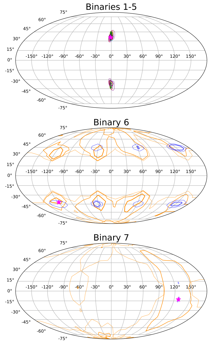
In terms of the ecliptic longitude and latitude, we observe what is generally expected. Figure 6 shows the 1-3 contours for the sky localization of each binary. For Binaries 1-5, with strong SNRs, signal at higher frequencies, and measurements of higher modes, we are able to precisely identify the ecliptic longitude, while strongly recovering the ecliptic latitude. Also, as expected, we are unable to differentiate between between above and below the LISA orbital plane, even though more posterior weight is located at the correct latitudinal mode. The relative level to which we constrained the sky location for Binaries 1-5 is determined by their SNR, modulated slightly by the randomness of the noise.
The sky localization achieved for the large binary is effectively minimal. This lack of localization in this specific case is due to Binary 6 existing in a near-edge-on configuration. In an edge-on configuration, the information from higher modes in terms of constraining the sky location is minimized. With the same binary injection parameters but an inclination in a more face-on configuration (), the sky localization is reduced to the eight degenerate sky modes expected for binaries at lower frequencies (see Marsat et al. 2020). This configuration is shown for reference in Figure 6. In this specific case, seven of the eight modes are highlighted. The frequency spectrum for Binary 6 does not extend to high enough frequencies to constrain the longitude to one of the four longitudinal modes. However, if this binary was run in the “spin up” configuration performed for Binary 4, the frequency-domain spectrum would extend high enough allowing the localization to narrow to one longitudinal mode. We also observe uncertainty as to whether the source is truly above or below the plane.
Similar to the large binary, the sky location constraint for the small binary is weak. This is also due to the edge-on configuration. When analyzed in a more face-on configuration (), the sky localization is much smaller, locating the correct longitudinal mode as is expected for a high-frequency binary. The sampler also located the correct latitude, but confusion as to whether the source is above or below the plane does exist. This face-on configuration is also shown in Figure 6 for reference.
The other extrinsic orientation parameters follow a predictable structure related to the ecliptic longitude and latitude. The inclination is reflected at and is reflected at . Additionally, since more than one longitudinal mode is observed for binary 6, is observed at deviations of from both the true and reflected values. Binaries 1-5 show Gaussian distributions for , and . However, it can be seen that correlates similarly to as they both depend on the intrinsic parameters in terms of setting the reference frequency at which these values are set.
The large binary is the only injection where the reference time is not constrained well (see Figure 12). Since the merger and ringdown are short relative to an inspiral evolution, the movement of the LISA constellation, as well as its rotation, is small during the observation of this signal. We are effectively observing a snapshot of the temporal aspect of the response function; therefore, moving the binary forward or backward in time will not change the response of the spacecraft by much, especially since we are operating on the order of seconds for the reference time parameter. The behavior of is reflective of the unique spin behavior detailed previously: directly correlates with the abnormal distribution for . Similar to the spin distributions, this is due to the setting of the reference frequency at which this phase is assigned. The luminosity distance for the large binary is constrained to within Gpc and shows the mean value and main peak near the injection value. However, the distribution of the distance measurements is not Gaussian, tending towards higher distances. Without much inspiral signal, we lose information that helps to constrain the distance to the binary.
We are able to constrain for the small binary quite well due to its long evolution in band (see Figure 13). seems to show a “split” posterior. However, it is really a symptom of wrapping the phase at 2. If we were to unwrap those posteriors, the areas that seem to be disjointed and separated would fit as one multi-modal posterior similar to those shown for the intrinsic parameters. The distance posterior for the small binary is unique. Similar to the large binary, this posterior tends towards larger distances than the injection. A difference with the small binary is that the mean value and main peak is not located at the true injection value. Since this binary is analyzed in a zero-noise representation, the random nature of noise did not cause this deviation. Without any noise, the maximum likelihood value would be found at the true distance value. However, since we do not see a main peak around this value, it means the parameter space volume centered around the true value does not contain a high percentage of posterior weight; our observations show there is more posterior weight around Gpc.
V Conclusion
We present the first noise-infused analysis of MBH binaries with LISA employing full waveforms spanning inspiral, merger, and ringdown that include higher order harmonic modes. Additionally, we expand on previous work by adding the inclusion of aligned spins. This study was performed with PhenomHM (London et al. 2018) and the fast frequency domain response from Marsat and Baker 2018. Both of these processes, as well as the likelihood computation, were accelerated with GPUs, which is a first for the LISA response function. We showed the extreme improvement in speed these GPU devices achieve. In instances where full data streams are analyzed with noise-infused injections, GPUs can achieve speeds or more times faster than a single CPU.
With these accelerated likelihood computations, we used Bayesian inference techniques to extract full marginalized posterior distributions across the dimensional parameter space. In particular, we employed a parallel-tempered implementation of the stretch proposal MCMC sampler implemented in Vousden et al. 2016.
We obtained full posterior distributions for 7 test binaries, which can be seen in Figures 7 - 13 in Section A of the Appendix. The parameters of the test binaries can be seen in Table 2. For the intrinsic parameters, , , and we show the recovered parameter values and their 1 errors in Tables 4-6. The errors generally follow proportionally to the SNR. However, when we fix the spins for Binary 3, we can further constrain the reference values because the spins help determine the frequency at which the reference values are set.
We highlighted the correlation between and as it varied for the different binaries. They exhibited a positive (negative) correlation if the slope of the sensitivity curve near the merger, where most of the signal is accumulated, is negative (positive).
The large binary (Binary 6) exhibits unique posteriors in versus . We show this posterior exhibits a non-ellipsoidal structure that follows a slope similar to the mass ratio (see Figure 5). Since the large binary signal is observed during only the merger and ringdown, this binary is more susceptible to likelihood changes when the secondary mass-weighted spin begins to dominate over the primary.
The small binary (Binary 7) shows a multi-modal distribution most likely due to its lower SNR and lack of strong observation of higher order modes.
We also discuss our ability to localize each binary (see Figure 6). The inclination of the binary holds strong influence over its localization. Face-on configurations provided much better sky localization for all binaries compared to edge-on configurations.
In future work, we plan to expand on the findings shown here by growing the binary parameter space that we have looked at, focusing on astrophysically motivated catalogs. Additionally, we will examine how the sky localization for a binary changes over time with the new LISA sensitivity curve, as well as with newer, advanced waveforms like PhenomHM , such as the coming waveform family for PhenomX (Pratten et al. 2020; García-Quirós et al. 2020; Pratten et al. 2020).
With this work, we see the aligned spins add a new dimension to the sampling of binaries resulting in interesting configurations in spin posteriors, as well as varying the constraints on the other parameters. We see that injected noise, as expected, has varied our ability to recover parameters. The analysis of these noise injections was made possible by the implementation of GPU-accelerated likelihood calculations, a tool that will help to further the reach of these parameter estimation studies in the run up to the launch of the LISA mission.
Acknowledgements.
M.L.K. acknowledges support from the National Science Foundation under grant DGE-0948017 and the Chateaubriand Fellowship from the Office for Science & Technology of the Embassy of France in the United States. M.L.K. would like to thank folks at the Labortatoire Astroparticule & Cosmologie in Paris, including Edward K. Porter, Marc Arene, Calum Murray, and the LISA group at APC for being gracious hosts. A.J.K.C. acknowledges support from the Jet Propulsion Laboratory Research and Technology Development program. This research was supported in part through the computational resources and staff contributions provided for the Quest/Grail high performance computing facility at Northwestern University. Astropy, a community-developed core Python package for Astronomy, was used in this research (Astropy Collaboration et al. 2013). Parts of this research were carried out at the Jet Propulsion Laboratory, California Institute of Technology, under a contract with the National Aeronautics and Space Administration (80NM0018D0004). This paper also employed use of Scipy (Jones et al.), Numpy (van der Walt et al. 2011), and Matplotlib (Hunter 2007).References
- Amaro-Seoane et al (2017) P. Amaro-Seoane et al, Laser Interferometer Space Antenna, ArXiv e-prints (2017), arXiv:1702.00786 [astro-ph.IM] .
- The LIGO Scientific Collaboration and the Virgo Collaboration (2018) The LIGO Scientific Collaboration and the Virgo Collaboration, GWTC-1: A Gravitational-Wave Transient Catalog of Compact Binary Mergers Observed by LIGO and Virgo during the First and Second Observing Runs, arXiv e-prints , arXiv:1811.12907 (2018), arXiv:1811.12907 [astro-ph.HE] .
- LVK Collaboration (2018) LVK Collaboration, Prospects for observing and localizing gravitational-wave transients with Advanced LIGO, Advanced Virgo and KAGRA, Living Reviews in Relativity 21, 3 (2018), arXiv:1304.0670 [gr-qc] .
- Klein et al. (2016) A. Klein, E. Barausse, A. Sesana, A. Petiteau, E. Berti, S. Babak, J. Gair, S. Aoudia, I. Hinder, F. Ohme, and B. Wardell, Science with the space-based interferometer eLISA: Supermassive black hole binaries, Phys. Rev. D 93, 24003 (2016), arXiv:1511.05581 [gr-qc] .
- Berti et al. (2016) E. Berti, A. Sesana, E. Barausse, V. Cardoso, and K. Belczynski, Spectroscopy of Kerr Black Holes with Earth- and Space-Based Interferometers, Phys. Rev. Lett. 117, 101102 (2016), arXiv:1605.09286 [gr-qc] .
- Salcido et al. (2016) J. Salcido, R. Bower, T. Theuns, S. McAlpine, M. Schaller, R. Crain, J. Schaye, and J. Regan, Music from the heavens - gravitational waves from supermassive black hole mergers in the EAGLE simulations, MNRAS 463, 870 (2016), arXiv:1601.06156 .
- Katz et al. (2019) M. L. Katz, L. Z. Kelley, F. Dosopoulou, S. Berry, L. Blecha, and S. L. Larson, Probing Massive Black Hole Binary Populations with LISA, arXiv e-prints , arXiv:1908.05779 (2019), arXiv:1908.05779 [astro-ph.HE] .
- Bonetti et al. (2019) M. Bonetti, A. Sesana, F. Haardt, E. Barausse, and M. Colpi, Post-Newtonian evolution of massive black hole triplets in galactic nuclei - IV. Implications for LISA, MNRAS 486, 4044 (2019), arXiv:1812.01011 [astro-ph.GA] .
- eLISA Consortium (2013) eLISA Consortium, The Gravitational Universe, arXiv e-prints , arXiv:1305.5720 (2013), arXiv:1305.5720 [astro-ph.CO] .
- Barausse et al. (2015) E. Barausse, J. Bellovary, E. Berti, B. Holley-Bockelmann K. Farris, B. Sathyaprakash, and A. Sesana, Massive Black Hole Science with eLISA, J. Phys.: Conf. Ser. 610, 12001 (2015).
- Katz and Larson (2019) M. Katz and S. Larson, Evaluating black hole detectability with LISA, MNRAS 483, 3108 (2019), arXiv:1807.02511 [gr-qc] .
- Loeb and Rasio (1994) A. Loeb and F. Rasio, Collapse of primordial gas clouds and the formation of quasar black holes, Astrophys. J. 432, 52 (1994).
- Begelman et al. (2006) M. Begelman, M. Volonteri, and M. Rees, Formation of supermassive black holes by direct collapse in pre-galactic haloes, MNRAS 370, 289 (2006).
- Latif et al. (2013) M. Latif, D. Schleicher, W. Schmidt, and J. Niemeyer, The characteristic black hole mass resulting from direct collapse in the early Universe, MNRAS 436, 2989 (2013), arXiv:1309.1097 .
- Habouzit et al. (2016) M. Habouzit, M. Volonteri, M. Latif, Y. Dubois, and S. Peirani, On the number density of ‘direct collapse’ black hole seeds, MNRAS 463, 529 (2016), arXiv:1601.00557 .
- Ardaneh et al. (2018) K. Ardaneh, Y. Luo, I. Shlosman, K. Nagamine, J. Wise, and M. Begelman, Direct Collapse to Supermassive Black Hole Seeds with Radiation Transfer: Cosmological Halos, ArXiv e-prints (2018), arXiv:1803.03278 .
- Dunn et al. (2018) G. Dunn, J. Bellovary, K. Holley-Bockelmann, C. Christensen, and T. Quinn, Sowing Black Hole Seeds: Direct Collapse Black Hole Formation with Realistic Lyman-Werner Radiation in Cosmological Simulations, Astrophys. J. 861, 39 (2018), arXiv:1803.01007 .
- Omukai et al. (2008) K. Omukai, R. Schneider, and Z. Haiman, Can Supermassive Black Holes Form in Metal-enriched High-Redshift Protogalaxies?, Astrophys. J. 686, 801 (2008), arXiv:0804.3141 .
- Devecchi and Volonteri (2009) B. Devecchi and M. Volonteri, Formation of the First Nuclear Clusters and Massive Black Holes at High Redshift, Astrophys. J. 694, 302 (2009), arXiv:0810.1057 .
- Davies et al. (2011) M. B. Davies, M. C. Miller, and J. M. Bellovary, Supermassive Black Hole Formation Via Gas Accretion in Nuclear Stellar Clusters, Astro 740, L42 (2011), arXiv:1106.5943 [astro-ph.CO] .
- Katz et al. (2015) H. Katz, D. Sijacki, and M. Haehnelt, Seeding high-redshift QSOs by collisional runaway in primordial star clusters, MNRAS 451, 2352 (2015), arXiv:1502.03448 .
- Haiman et al. (2000) Z. Haiman, T. Abel, and M. Rees, The Radiative Feedback of the First Cosmological Objects, Astrophys. J. 534, 11 (2000).
- Fryer et al. (2001) C. Fryer, S. Woosley, and A. Heger, Pair-Instability Supernovae, Gravity Waves, and Gamma-Ray Transients, Astrophys. J. 550, 372 (2001).
- Heger et al. (2003) A. Heger, C. Fryer, S. Woosley, N. Langer, and D. Hartmann, How Massive Single Stars End Their Life, Astrophys. J. 591, 288 (2003).
- Volonteri et al. (2003) M. Volonteri, P. Madau, and F. Haardt, The Formation of Galaxy Stellar Cores by the Hierarchical Merging of Supermassive Black Holes, Astrophys. J. 593, 661 (2003).
- Tanaka and Haiman (2009) T. Tanaka and Z. Haiman, The Assembly of Supermassive Black Holes at High Redshifts, Astrophys. J. 696, 1798 (2009), arXiv:0807.4702 .
- Alvarez et al. (2009) M. A. Alvarez, J. H. Wise, and T. Abel, ACCRETION ONTO THE FIRST STELLAR-MASS BLACK HOLES, The Astrophysical Journal 701, L133 (2009).
- Petiteau et al. (2011) A. Petiteau, S. Babak, and A. Sesana, Constraining the Dark Energy Equation of State Using LISA Observations of Spinning Massive Black Hole Binaries, Astrophys. J. 732, 82 (2011), arXiv:1102.0769 .
- Gair et al. (2013) J. Gair, M. Vallisneri, S. Larson, and J. Baker, Testing General Relativity with Low-Frequency, Space-Based Gravitational-Wave Detectors, Living Reviews in Relativity 16, 7 (2013), arXiv:1212.5575 [gr-qc] .
- Schutz (1986) B. Schutz, Determining the Hubble constant from gravitational wave observations, Nature (London) 323, 310 (1986).
- Holz and Hughes (2005) D. E. Holz and S. A. Hughes, Using Gravitational-Wave Standard Sirens, Astrophys. J. 629, 15 (2005), arXiv:astro-ph/0504616 [astro-ph] .
- Armitage and Natarajan (2002) P. J. Armitage and P. Natarajan, Accretion during the Merger of Supermassive Black Holes, Astro 567, L9 (2002), arXiv:astro-ph/0201318 [astro-ph] .
- Burke-Spolaor (2013) S. Burke-Spolaor, Multi-messenger approaches to binary supermassive black holes in the ‘continuous-wave’ regime, Classical and Quantum Gravity 30, 224013 (2013), arXiv:1308.4408 [astro-ph.CO] .
- Bogdanović (2015) T. Bogdanović, Supermassive Black Hole Binaries: The Search Continues, in Gravitational Wave Astrophysics, Vol. 40 (2015) p. 103, arXiv:1406.5193 [astro-ph.HE] .
- Dal Canton et al. (2019) T. Dal Canton, A. Mangiagli, S. C. Noble, J. Schnittman, A. Ptak, A. Klein, A. Sesana, and J. Camp, Detectability of Modulated X-Rays from LISA’s Supermassive Black Hole Mergers, Astrophys. J. 886, 146 (2019), arXiv:1902.01538 [astro-ph.HE] .
- Cornish and Porter (2006) N. J. Cornish and E. K. Porter, MCMC exploration of supermassive black hole binary inspirals, Classical and Quantum Gravity 23, S761 (2006), arXiv:gr-qc/0605085 [gr-qc] .
- Cornish and Porter (2007) N. J. Cornish and E. K. Porter, Catching supermassive black hole binaries without a net, Phys. Rev. D 75, 21301 (2007), arXiv:gr-qc/0605135 [gr-qc] .
- Porter and Carré (2014) E. K. Porter and J. Carré, A Hamiltonian Monte-Carlo method for Bayesian inference of supermassive black hole binaries, Classical and Quantum Gravity 31, 145004 (2014), arXiv:1311.7539 [gr-qc] .
- Porter and Cornish (2015) E. K. Porter and N. J. Cornish, Fisher versus Bayes: A comparison of parameter estimation techniques for massive black hole binaries to high redshifts with eLISA, Phys. Rev. D 91, 104001 (2015), arXiv:1502.05735 [gr-qc] .
- Marsat et al. (2020) S. Marsat, J. G. Baker, and T. Dal Canton, Exploring the Bayesian parameter estimation of binary black holes with LISA, arXiv e-prints , arXiv:2003.00357 (2020), arXiv:2003.00357 [gr-qc] .
- Christensen and Meyer (1998) N. Christensen and R. Meyer, Markov chain Monte Carlo methods for Bayesian gravitational radiation data analysis, Phys. Rev. D 58, 82001 (1998).
- Porter and Cornish (2008) E. K. Porter and N. J. Cornish, Effect of higher harmonic corrections on the detection of massive black hole binaries with LISA, Phys. Rev. D 78, 64005 (2008), arXiv:0804.0332 [gr-qc] .
- Vallisneri (2008) M. Vallisneri, Use and abuse of the Fisher information matrix in the assessment of gravitational-wave parameter-estimation prospects, Phys. Rev. D 77, 42001 (2008), arXiv:gr-qc/0703086 [gr-qc] .
- Cutler and Vallisneri (2007) C. Cutler and M. Vallisneri, LISA detections of massive black hole inspirals: Parameter extraction errors due to inaccurate template waveforms, Phys. Rev. D 76, 104018 (2007), arXiv:0707.2982 [gr-qc] .
- Team (2018) L. S. S. Team, LISA Science Requirements Document (2018).
- Cutler and Flanagan (1994) C. Cutler and É. Flanagan, Gravitational waves from merging compact binaries: How accurately can one extract the binary’s parameters from the inspiral waveform?, Phys. Rev. D 49, 2658 (1994).
- Vecchio (2004) A. Vecchio, LISA observations of rapidly spinning massive black hole binary systems, Phys. Rev. D 70, 42001 (2004), arXiv:astro-ph/0304051 [astro-ph] .
- Arun (2006) K. Arun, Parameter estimation of coalescing supermassive black hole binaries with LISA, Phys. Rev. D 74, 24025 (2006), arXiv:gr-qc/0605021 [gr-qc] .
- Berti et al. (2005) E. Berti, A. Buonanno, and C. M. Will, Estimating spinning binary parameters and testing alternative theories of gravity with LISA, Phys. Rev. D 71, 84025 (2005), arXiv:gr-qc/0411129 [gr-qc] .
- Lang and Hughes (2006) R. N. Lang and S. A. Hughes, Measuring coalescing massive binary black holes with gravitational waves: The impact of spin-induced precession, Phys. Rev. D 74, 122001 (2006), arXiv:gr-qc/0608062 [gr-qc] .
- Babak et al. (2010) S. Babak, J. G. Baker, M. J. Benacquista, N. J. Cornish, S. L. Larson, I. Mandel, S. T. McWilliams, A. Petiteau, E. K. Porter, E. L. Robinson, M. Vallisneri, A. Vecchio, t. M. L. Data Challenge Task Force, M. Adams, K. A. Arnaud, A. Błaut, M. Bridges, M. Cohen, C. Cutler, F. Feroz, J. R. Gair, P. Graff, M. Hobson, J. Shapiro Key, A. Królak, A. Lasenby, R. Prix, Y. Shang, M. Trias, J. Veitch, J. T. Whelan, and t. C. . Participants, The Mock LISA Data Challenges: from challenge 3 to challenge 4, Classical and Quantum Gravity 27, 84009 (2010), arXiv:0912.0548 [gr-qc] .
- Brown et al. (2007) D. A. Brown, J. Crowder, C. Cutler, I. Mand el, and M. Vallisneri, A three-stage search for supermassive black-hole binaries in LISA data, Classical and Quantum Gravity 24, S595 (2007), arXiv:0704.2447 [gr-qc] .
- Crowder et al. (2006) J. Crowder, N. J. Cornish, and J. L. Reddinger, LISA data analysis using genetic algorithms, Phys. Rev. D 73, 63011 (2006), arXiv:gr-qc/0601036 [gr-qc] .
- Wickham et al. (2006) E. Wickham, A. Stroeer, and A. Vecchio, A Markov chain Monte Carlo approach to the study of massive black hole binary systems with LISA, Classical and Quantum Gravity 23, S819 (2006), arXiv:gr-qc/0605071 [gr-qc] .
- Röver et al. (2007) C. Röver, A. Stroeer, E. Bloomer, N. Christensen, J. Clark, M. Hendry, C. Messenger, R. Meyer, M. Pitkin, J. Toher, R. Umstätter, A. Vecchio, J. Veitch, and G. Woan, Inference on inspiral signals using LISA MLDC data, Classical and Quantum Gravity 24, S521 (2007), arXiv:0707.3969 [gr-qc] .
- Feroz et al. (2009) F. Feroz, J. R. Gair, M. P. Hobson, and E. K. Porter, Use of the MULTINEST algorithm for gravitational wave data analysis, Classical and Quantum Gravity 26, 215003 (2009), arXiv:0904.1544 [gr-qc] .
- Gair and Porter (2009) J. R. Gair and E. K. Porter, Cosmic swarms: a search for supermassive black holes in the LISA data stream with a hybrid evolutionary algorithm, Classical and Quantum Gravity 26, 225004 (2009), arXiv:0903.3733 [gr-qc] .
- Petiteau et al. (2009) A. Petiteau, Y. Shang, and S. Babak, The search for black hole binaries using a genetic algorithm, Classical and Quantum Gravity 26, 204011 (2009), arXiv:0905.1785 [gr-qc] .
- Arun et al. (2007) K. Arun, B. R. Iyer, B. Sathyaprakash, S. Sinha, and C. van den Broeck, Higher signal harmonics, LISA’s angular resolution, and dark energy, Phys. Rev. D 76, 104016 (2007), arXiv:0707.3920 [astro-ph] .
- Trias and Sintes (2008) M. Trias and A. M. Sintes, LISA observations of supermassive black holes: Parameter estimation using full post-Newtonian inspiral waveforms, Phys. Rev. D 77, 24030 (2008), arXiv:0707.4434 [gr-qc] .
- McWilliams et al. (2010a) S. T. McWilliams, J. I. Thorpe, J. G. Baker, and B. J. Kelly, Impact of mergers on LISA parameter estimation for nonspinning black hole binaries, Phys. Rev. D 81, 64014 (2010a), arXiv:0911.1078 [gr-qc] .
- Thorpe et al. (2009) J. Thorpe, S. McWilliams, B. Kelly, R. Fahey, K. Arnaud, and J. Baker, LISA parameter estimation using numerical merger waveforms, Classical and Quantum Gravity 26, 94026 (2009), arXiv:0811.0833 [astro-ph] .
- McWilliams et al. (2010b) S. T. McWilliams, B. J. Kelly, and J. G. Baker, Observing mergers of nonspinning black-hole binaries, Phys. Rev. D 82, 24014 (2010b), arXiv:1004.0961 [gr-qc] .
- McWilliams et al. (2011) S. McWilliams, R. Lang, J. Baker, and J. Thorpe, Sky localization of complete inspiral-merger-ringdown signals for nonspinning massive black hole binaries, Phys. Rev. D 84, 64003 (2011), arXiv:1104.5650 [gr-qc] .
- Babak et al. (2008) S. Babak, M. Hannam, S. Husa, and B. Schutz, Resolving Super Massive Black Holes with LISA, arXiv e-prints , arXiv:0806.1591 (2008), arXiv:0806.1591 [gr-qc] .
- Babak et al. (2014) S. Babak, J. Gair, and R. Cole, Extreme mass ratio inspirals: perspectives for their detection, ArXiv e-prints (2014), arXiv:1411.5253 [gr-qc] .
- Baibhav et al. (2020) V. Baibhav, E. Berti, and V. Cardoso, LISA parameter estimation and source localization with higher harmonics of the ringdown, arXiv e-prints , arXiv:2001.10011 (2020), arXiv:2001.10011 [gr-qc] .
- Marsat and Baker (2018) S. Marsat and J. G. Baker, Fourier-domain modulations and delays of gravitational-wave signals, arXiv e-prints , arXiv:1806.10734 (2018), arXiv:1806.10734 [gr-qc] .
- Larson et al. (2000) S. Larson, W. Hiscock, and R. Hellings, Sensitivity curves for spaceborne gravitational wave interferometers, Phys. Rev. D 62, 62001 (2000).
- Husa et al. (2016) S. Husa, S. Khan, M. Hannam, M. Pürrer, F. Ohme, X. Forteza, and A. Bohé, Frequency-domain gravitational waves from nonprecessing black-hole binaries. I. New numerical waveforms and anatomy of the signal, Phys. Rev. D 93, 44006 (2016), arXiv:1508.07250 [gr-qc] .
- Khan et al. (2016) S. Khan, S. Husa, M. Hannam, F. Ohme, M. Pürrer, X. Forteza, and A. Bohé, Frequency-domain gravitational waves from nonprecessing black-hole binaries. II. A phenomenological model for the advanced detector era, Phys. Rev. D 93, 44007 (2016), arXiv:1508.07253 [gr-qc] .
- Cornish and Robson (2018) N. Cornish and T. Robson, The construction and use of LISA sensitivity curves, ArXiv e-prints (2018), arXiv:1803.01944 [astro-ph.HE] .
- Amaro-Seoane et al. (2017) P. Amaro-Seoane, H. Audley, S. Babak, J. Baker, E. Barausse, P. Bender, E. Berti, P. Binetruy, M. Born, D. Bortoluzzi, J. Camp, C. Caprini, V. Cardoso, M. Colpi, J. Conklin, N. Cornish, C. Cutler, K. Danzmann, R. Dolesi, L. Ferraioli, V. Ferroni, E. Fitzsimons, J. Gair, L. Gesa Bote, D. Giardini, F. Gibert, C. Grimani, H. Halloin, G. Heinzel, T. Hertog, M. Hewitson, K. Holley-Bockelmann, D. Hollington, M. Hueller, H. Inchauspe, P. Jetzer, N. Karnesis, C. Killow, A. Klein, B. Klipstein, N. Korsakova, S. Larson, J. Livas, I. Lloro, N. Man, D. Mance, J. Martino, I. Mateos, K. McKenzie, S. McWilliams, C. Miller, G. Mueller, G. Nardini, G. Nelemans, M. Nofrarias, A. Petiteau, P. Pivato, E. Plagnol, E. Porter, J. Reiche, D. Robertson, N. Robertson, E. Rossi, G. Russano, B. Schutz, A. Sesana, D. Shoemaker, J. Slutsky, C. Sopuerta, T. Sumner, N. Tamanini, I. Thorpe, M. Troebs, M. Vallisneri, A. Vecchio, D. Vetrugno, S. Vitale, M. Volonteri, G. Wanner, H. Ward, P. Wass, W. Weber, J. Ziemer, and P. Zweifel, Laser Interferometer Space Antenna, ArXiv e-prints (2017), arXiv:1702.00786 [astro-ph.IM] .
- Finn and Thorne (2000) L. Finn and K. Thorne, Gravitational waves from a compact star in a circular, inspiral orbit, in the equatorial plane of a massive, spinning black hole, as observed by LISA, Phys. Rev. D 62, 124021 (2000).
- Moore et al. (2015) C. J. Moore, R. H. Cole, and C. P. L. Berry, Gravitational-wave sensitivity curves, Classical and Quantum Gravity 32, 15014 (2015).
- London et al. (2018) L. London, S. Khan, E. Fauchon-Jones, C. García, M. Hannam, S. Husa, X. Jiménez-Forteza, C. Kalaghatgi, F. Ohme, and F. Pannarale, First Higher-Multipole Model of Gravitational Waves from Spinning and Coalescing Black-Hole Binaries, Physical Review Letters 120, 161102 (2018), arXiv:1708.00404 [gr-qc] .
- Babak et al. (2017) S. Babak, J. Gair, A. Sesana, E. Barausse, C. Sopuerta, C. Berry, E. Berti, P. Amaro-Seoane, A. Petiteau, and A. Klein, Science with the space-based interferometer LISA. V. Extreme mass-ratio inspirals, Phys. Rev. D 95, 3012 (2017).
- Edwards et al. (2015) M. C. Edwards, R. Meyer, and N. Christensen, Bayesian semiparametric power spectral density estimation with applications in gravitational wave data analysis, Phys. Rev. D 92, 064011 (2015).
- Littenberg and Cornish (2015) T. B. Littenberg and N. J. Cornish, Bayesian inference for spectral estimation of gravitational wave detector noise, Phys. Rev. D 91, 084034 (2015).
- Biscoveanu et al. (2020) S. Biscoveanu, C.-J. Haster, S. Vitale, and J. Davies, Quantifying the Effect of Power Spectral Density Uncertainty on Gravitational-Wave Parameter Estimation for Compact Binary Sources, arXiv e-prints , arXiv:2004.05149 (2020), arXiv:2004.05149 [astro-ph.HE] .
- Goggans and Chi (2004) P. M. Goggans and Y. Chi, Using thermodynamic integration to calculate the posterior probability in bayesian model selection problems, AIP Conference Proceedings 707, 59 (2004), https://aip.scitation.org/doi/pdf/10.1063/1.1751356 .
- Lartillot and Philippe (2006) N. Lartillot and H. Philippe, Computing Bayes Factors Using Thermodynamic Integration, Systematic Biology 55, 195 (2006), https://academic.oup.com/sysbio/article-pdf/55/2/195/26557316/10635150500433722.pdf .
- Maturana-Russel et al. (2019) P. Maturana-Russel, R. Meyer, J. Veitch, and N. Christensen, Stepping-stone sampling algorithm for calculating the evidence of gravitational wave models, Phys. Rev. D 99, 084006 (2019), arXiv:1810.04488 [physics.data-an] .
- Kalaghatgi et al. (2019) C. Kalaghatgi, M. Hannam, and V. Raymond, Parameter Estimation with a spinning multi-mode waveform model: IMRPhenomHM, arXiv e-prints , arXiv:1909.10010 (2019), arXiv:1909.10010 [gr-qc] .
- Cornish and Rubbo (2003) N. J. Cornish and L. J. Rubbo, Publisher’s Note: LISA response function [Phys. Rev. D 67, 022001 (2003)], Phys. Rev. D 67, 29905 (2003), arXiv:gr-qc/0209011 [gr-qc] .
- Tinto and Armstrong (1999) M. Tinto and J. W. Armstrong, Cancellation of laser noise in an unequal-arm interferometer detector of gravitational radiation, Phys. Rev. D 59, 102003 (1999).
- Armstrong et al. (1999) J. Armstrong, F. Estabrook, and M. Tinto, Time-Delay Interferometry for Space-based Gravitational Wave Searches, Astrophys. J. 527, 814 (1999).
- Estabrook et al. (2000) F. B. Estabrook, M. Tinto, and J. W. Armstrong, Time-delay analysis of LISA gravitational wave data: Elimination of spacecraft motion effects, Phys. Rev. D 62, 42002 (2000).
- Dhurandhar et al. (2002) S. V. Dhurandhar, K. R. Nayak, and J.-Y. Vinet, Algebraic approach to time-delay data analysis for LISA, Phys. Rev. D 65, 102002 (2002).
- Tinto and Dhurandhar (2005) M. Tinto and S. V. Dhurandhar, Time-Delay Interferometry, Living Reviews in Relativity 8, 4 (2005).
- Vallisneri (2005) M. Vallisneri, Synthetic LISA: Simulating time delay interferometry in a model LISA, Phys. Rev. D 71, 22001 (2005), arXiv:gr-qc/0407102 [gr-qc] .
- Tinto and Dhurandhar (2014) M. Tinto and S. V. Dhurandhar, Time-Delay Interferometry, Living Reviews in Relativity 17, 6 (2014).
- Muratore et al. (2020) M. Muratore, D. Vetrugno, and S. Vitale, Revisitation of time delay interferometry combinations that suppress laser noise in LISA, arXiv e-prints , arXiv:2001.11221 (2020), arXiv:2001.11221 [astro-ph.IM] .
- Nickolls et al. (2008) J. Nickolls, I. Buck, M. Garland, and K. Skadron, Scalable Parallel Programming with CUDA, Queue 6, 40 (2008).
- Talbot et al. (2019) C. Talbot, R. Smith, E. Thrane, and G. B. Poole, Parallelized Inference for Gravitational-Wave Astronomy, arXiv e-prints , arXiv:1904.02863 (2019), arXiv:1904.02863 [astro-ph.IM] .
- Hannam et al. (2014) M. Hannam, P. Schmidt, A. Bohé, L. Haegel, S. Husa, F. Ohme, G. Pratten, and M. Pürrer, Simple Model of Complete Precessing Black-Hole-Binary Gravitational Waveforms, Phys. Rev. Lett. 113, 151101 (2014).
- LIGO Scientific Collaboration (2018) LIGO Scientific Collaboration, LIGO Algorithm Library - LALSuite, free software (GPL) (2018).
- (98) E. Jones, T. Oliphant, P. Peterson, and Others, SciPy: Open source scientific tools for Python.
- (99) cusparse, https://docs.nvidia.com/cuda/cusparse/index.html, [Online; accessed 2019-8-25].
- (100) cuBLAS, https://docs.nvidia.com/cuda/cublas/index.html, [Online; accessed 2019-8-25].
- Behnel et al. (2011) S. Behnel, R. Bradshaw, C. Citro, L. Dalcin, D. S. Seljebotn, and K. Smith, Cython: The best of both worlds, Computing in Science & Engineering 13, 31 (2011).
- (102) R. McGibbon and Y. Zhao, npcuda-example.
- Skilling (2004) J. Skilling, Nested Sampling, AIP Conference Proceedings 735, 395 (2004).
- Skilling (2006) J. Skilling, Nested sampling for general Bayesian computation, Bayesian Anal. 1, 833 (2006).
- Metropolis and Ulam (1949) N. Metropolis and S. Ulam, The Monte Carlo Method, Journal of the American Statistical Association 44, 335 (1949).
- Metropolis et al. (1953) N. Metropolis, A. W. Rosenbluth, M. N. Rosenbluth, A. H. Teller, and E. Teller, Equation of State Calculations by Fast Computing Machines, The Journal of Chemical Physics 21, 1087 (1953).
- Hastings (1970) W. K. Hastings, Monte Carlo sampling methods using Markov chains and their applications, Biometrika 57, 97 (1970).
- Foreman-Mackey et al. (2013) D. Foreman-Mackey, D. W. Hogg, D. Lang, and J. Goodman, emcee: The MCMC Hammer, Publications of the Astronomical Society of the Pacific 125, 306 (2013), arXiv:1202.3665 [astro-ph.IM] .
- Vousden et al. (2016) W. Vousden, W. Farr, and I. Mandel, Dynamic temperature selection for parallel tempering in Markov chain Monte Carlo simulations, MNRAS 455, 1919 (2016), arXiv:1501.05823 [astro-ph.IM] .
- Goodman and Weare (2010) J. Goodman and J. Weare, Ensemble samplers with affine invariance, Communications in Applied Mathematics and Computational Science, Vol.5, No.1, p.65-80, 2010 5, 65 (2010).
- Swendsen and Wang (1986) R. H. Swendsen and J.-S. Wang, Replica Monte Carlo simulation of spin glasses, Phys. Rev. Lett. 57, 2607 (1986).
- Earl and Deem (2005) D. J. Earl and M. W. Deem, Parallel tempering: Theory, applications, and new perspectives, Physical Chemistry Chemical Physics (Incorporating Faraday Transactions) 7, 3910 (2005), arXiv:physics/0508111 [physics.comp-ph] .
- Sokal (1997) A. Sokal, Monte Carlo Methods in Statistical Mechanics: Foundations and New Algorithms, in Functional Integration: Basics and Applications, edited by C. DeWitt-Morette, P. Cartier, and A. Folacci (Springer US, Boston, MA, 1997) pp. 131–192.
- Foreman-Mackey (2018) D. Foreman-Mackey, Autocorrelation time estimation, https://dfm.io/posts/autocorr/ (2018).
- Pratten et al. (2020) G. Pratten, S. Husa, C. Garcia-Quiros, M. Colleoni, A. Ramos-Buades, H. Estelles, and R. Jaume, Setting the cornerstone for the IMRPhenomX family of models for gravitational waves from compact binaries: The dominant harmonic for non-precessing quasi-circular black holes, arXiv e-prints , arXiv:2001.11412 (2020), arXiv:2001.11412 [gr-qc] .
- García-Quirós et al. (2020) C. García-Quirós, M. Colleoni, S. Husa, H. Estellés, G. Pratten, A. Ramos-Buades, M. Mateu-Lucena, and R. Jaume, IMRPhenomXHM: A multi-mode frequency-domain model for the gravitational wave signal from non-precessing black-hole binaries, arXiv e-prints , arXiv:2001.10914 (2020), arXiv:2001.10914 [gr-qc] .
- Pratten et al. (2020) G. Pratten, C. García-Quirós, M. Colleoni, A. Ramos-Buades, H. Estellés, M. Mateu-Lucena, R. Jaume, M. Haney, D. Keitel, J. E. Thompson, and S. Husa, Let’s twist again: computationally efficient models for the dominant and sub-dominant harmonic modes of precessing binary black holes, arXiv e-prints , arXiv:2004.06503 (2020), arXiv:2004.06503 [gr-qc] .
- Astropy Collaboration et al. (2013) Astropy Collaboration, T. Robitaille, E. Tollerud, P. Greenfield, M. Droettboom, E. Bray, T. Aldcroft, M. Davis, A. Ginsburg, A. Price-Whelan, W. Kerzendorf, A. Conley, N. Crighton, K. Barbary, D. Muna, H. Ferguson, F. Grollier, M. Parikh, P. Nair, H. Unther, C. Deil, J. Woillez, S. Conseil, R. Kramer, J. Turner, L. Singer, R. Fox, B. Weaver, V. Zabalza, Z. Edwards, K. Azalee Bostroem, D. Burke, A. Casey, S. Crawford, N. Dencheva, J. Ely, T. Jenness, K. Labrie, P. Lim, F. Pierfederici, A. Pontzen, A. Ptak, B. Refsdal, M. Servillat, and O. Streicher, Astropy: A community Python package for astronomy, Astronomy & Astrophysics 558, A33 (2013), arXiv:1307.6212 [astro-ph.IM] .
- van der Walt et al. (2011) S. van der Walt, S. C. Colbert, and G. Varoquaux, The NumPy Array: A Structure for Efficient Numerical Computation, Computing In Science & Engineering 13, 22 (2011).
- Hunter (2007) J. D. Hunter, Matplotlib: A 2D graphics environment, Computing In Science & Engineering 9, 90 (2007).
Appendix A Posterior Distributions
Here we present the full corner plots for all binaries tested (see Table 2) to accompany subsections of the corner plots shown in Section IV. Binaries 1-7 are shown in Figures 7 - 13, respectively. The exact injection parameters for each binary can be seen in Table 2, and are represented by a green point in the full posteriors. All sky position and orientation parameters are displayed over their entire domain (or prior range) due to their inherent multi-modal structure. The other parameters are shown zooming in on the distributions that account for 99.9% of marginalized posterior points. The inclination, , and ecliptic latitude, , are plotted as and because these are the parameters sampled during the MCMC runs. Similarly, the total mass, ; luminosity distance, ; and reference time, , are all sampled and plotted as the natural log of these values. Table 7 shows the autocorrelation time () and effective sample size (ESS) according to Section III.3 for each MCMC run. It also gives the average acceptance fraction (AF) for each run.
| Binary | ESS | AF | |
|---|---|---|---|
| 1 | 97 | 79200 | 0.20 |
| 2 | 93 | 103232 | 0.19 |
| 3 | 63 | 50816 | 0.25 |
| 4 | 90 | 67584 | 0.24 |
| 5 | 80 | 52000 | 0.19 |
| 6 | 45 | 64000 | 0.18 |
| 7 | 8 | 600000 | 0.21 |