Tractable learning in under-excited power grids
Abstract
Estimating the structure of physical flow networks such as power grids is critical to secure delivery of energy. This paper discusses statistical structure estimation in power grids in the ‘under-excited’ regime, where a subset of internal nodes do not have external injection. Prior estimation algorithms based on nodal potentials/voltages fail in the under-excited regime. We propose a novel topology learning algorithm for learning under-excited general (non-radial) networks based on physics-informed conservation laws. We prove the asymptotic correctness of our algorithm for grids with non-adjacent under-excited internal nodes. More importantly, we theoretically analyze our algorithm’s efficacy under noisy measurements, and determine bounds on maximum noise under which asymptotically correct recovery is guaranteed. Our approach is validated through simulations with non-linear voltage samples generated on test grids with real injection data.
Index Terms:
Flow conversation, Inverse graph Laplacian, noisy regression, Matpower, inverse covariance graph, distribution grid.I Introduction
Topology estimation is a crucial part of situational awareness in power grids, which is the backbone for energy needs in the modern economy [1]. Operationally the power grid can be distinguished between high voltage transmission grids and low voltage distribution grids [2]. Structurally, the transmissions are meshed/loopy (have cycles), while distributional grids are primarily radial (tree-like). In either setting, the grid topology is established by the status of breakers/switches on an underlying set of permissible lines/edges as shown in Fig. 1. In the modern grid, presence of stochastic resources such as solar energy, wind farms, and aggregated controllable loads have made topology and state estimation with guarantees of paramount importance for secure operation. In the absence of sufficient line measurements [3], in recent years, researchers [4] have proposed the use of nodal voltage measurements collected from new, high-fidelity nodal measurement devices such as PMUs [5], micro-pmus [6], and advanced metering equipment to aid in topology estimation. Among algorithms with theoretical guarantees, passive greedy schemes [1, 7, 8] and active probing methods [9, 10] that employ voltage measurements are proposed for learning radial grids. However, they do not generalize to meshed/loopy networks in transmission grids and urban distribution grids [11, 12]. Similarly, algorithms for joint estimation of topology and line parameters using both voltage and injection measurements have been designed using least-squared fitting [13] and low-ranked decomposition [14]. While these works are related, in this article we focus on the problem of topology recovery using only nodal voltage measurements without any additional measurement or statistics of nodal injections. In a related line of work, consistent algorithms based on inverse covariance or mutual independence (MI) of nodal voltages are used for learning grid topology in both radial [15, 16, 17], and loopy settings [18, 19]. Its theoretical generalizability notwithstanding, the validity of inverse voltage covariance or MI based methods rely on a key assumption: all nodes/buses are excited, i.e., have non-zero injection fluctuations. This is necessary to ensure that the voltage covariance matrix is full-ranked and hence invertible. While terminal nodes in grids generally have loads or generation, an unidentified set of internal nodes with zero injection may be present in realistic transmission and distribution grids for routing power flows [2]. In such setting, voltage measurement based learning algorithms proposed in prior work do not extend theoretically. The overarching goal of this work is to overcome this drawback and develop a provably correct topology learning algorithm using only nodal voltages from a general (loopy) power grid, where an unidentified subset of internal nodes may be unexcited. As linearized power flow models are examples of structural equation models (SEM) [20], our work enables tractable learning for SEMs satisfying conservation laws, in the under-excited regime, using only state samples. Extensions in systems beyond power grids are the objective of our future work.
I-A Contribution
Our learning algorithm is based on the physics of linearized power flows. As the voltage covariance matrix is rank-deficient in the under-excited regime, we propose a two-step learning approach. In the first step, we develop a regression based test that identifies the internal nodes of zero injection, and subsequently learns their true neighbors. In the second step, we extract the voltage covariance pertaining only to nodes with non-zero injection, and estimate the rest of the network. We prove that under noiseless measurements, our algorithm correctly estimates the underlying topology of radial grids, provided under-excited internal nodes are non-adjacent. For loopy grids of minimum loop-size four, our algorithm ensures correct learning provided loops of size four do not include zero-injection buses. Note that the minimum loop size of four is non-restrictive as real grids have large girth [11], and is necessary for correct estimation even in the fully-excited setting [19]. We show the necessity of our assumptions for unique and consistent recovery, through multiple counter examples. Under noisy data, we determine the maximum noise margin for consistency of each step of our learning algorithm, and express this margin as an intuitive function of system parameters. We validate the developed algorithms through experiments on both linear and non-linear voltage samples collected from test grids with real injection data.
The next section discusses power flows in grids and related voltage statistics. Section III discusses properties of nodal voltages which is used to extract zero-injection buses and their neighbors. Section IV determines edges between non-zero injection buses and completes the topology estimation. The analysis under noise for each step is provided in its corresponding section. Section V includes simulations results on IEEE test networks, using non-linear samples generated using real injection data. Conclusions and future work, are included in Section VI.

II Preliminaries
II-A Notation
We denote the power grid topology by an undirected graph , where is the set of nodes/nodes, and is the set of operational lines/edges (see Fig. 1). Two nodes that share an edge are termed ‘neighbors’. The degree of a node is the total number of edges that involve the node. A node with degree is termed a ‘terminal node’, and an ‘internal’ node otherwise. A ‘loop’ of size refers to a set of distinct edges . A radial (loop-less) graph is defined to have loops of minimum size . Each edge in grid is associated with susceptance , and conductance . Each node has a corresponding voltage magnitude , phase angle , active power and reactive power . We use to denote the corresponding vectors with entries for each node.
II-B Power grid basics
The Kirchoff’s law for AC power flow (AC-PF) is given by:
| (1) |
Considering small deviations in from a reference bus voltage and small differences in between neighboring nodes, the non-linear AC-PF can be linearized in to get the Linearized AC power flow (LC-PF) [1, 21, 22] whereby,
| (2) |
The susceptance weighted Laplacian matrix is given by
| (3) |
is defined similarly. If voltage magnitude deviations are negligible, or lines are primarily susceptive, the linear DC power flow (DC-PF), is derived [21]:
| (4) |
Note that both LC-PF and DC-PF models are lossless. One node’s voltage can be taken as reference to measure all other voltages, while its injection is given by the negative sum of all other injections. The PF models can then be reduced to the non-reference nodes by removing entries in , and rows and columns in that correspond to the reference node. From this point onwards, we use to refer to their reduced versions. As reduced have full rank, LC-PF and DC-PF models are invertible. In the rest of the article, we focus on DC-PF for our theoretical results. Our analysis naturally extends to the LC-PF model, as noted in subsequent sections. Furthermore, our simulations results demonstrate the performance of our learning algorithm on non-linear AC-PF voltage measurements.
II-C Structure recovery problem
The structure recovery problem pertains to estimating the set of edges of using the measurements of the phase angles (and voltages for the LC-PF model). For the theoretical analysis, we consider the asymptotic setting , that ensures sufficient number of collected voltage observations for correct estimation of the second order statistics of the nodal voltages. Our simulation results demonstrate the performance in the low-sample regime. In an under-excited grid , we denote the set of internal nodes with zero-injection by , and the remaining nodes in by , respectively. Without a loss of generality, we consider the nodes numbered to ( denotes the cardinality of set ) as zero-injection and rest as non-zero injection nodes. Thus, we partition , and . We assume the following regarding covariance nodal injections:
Assumption 1.
Fluctuations in are uncorrelated:
and is diagonal.
Assumption 1 is used in prior work [15, 16, 17] for tractable grid learning. Further it also holds for real loads and renewables [18, 23], when small linear trends are empirically de-trended. While Assumption 1 is used for proving the correctness of a part of our algorithm (Section IV), we consider real correlated injection data in our numerical simulations to demonstrate accurate learning, in its absence.
II-D The fully excited case
If is empty, and are invertible, and
| (6) |
Note that if are not part of a loop of size three, then they must exist in one of the configurations in Eq. (6). The following thus holds.
Lemma 1.
Note: In the LC-PF model [19], under faithfullness assumptions, it can be shown that if are not in a three-node loop, exists iff .
If the minimum loop size for grid is four, no node pair exists in a three-node loop. Thus, Lemma 1 enables correct topology estimation in the fully-excited setting [16, 19], under both DC-PF and LC-PF. Noteably, Lemma 1 fails in the under-exited regime as or are not invertible. The rest of the paper discusses tractable learning in this under-excited setting. To learn grids with zero-injection node set , we propose a two-step topology learning algorithm. First, we identify zero injection nodes and their neighbors. Next, we estimate edges between node pairs with non-zero injection. The next section presents a regression-based framework for the first step.
III Identifying zero-injection nodes and neighbors
We first start with stating the required assumption for structure recovery in the under-excited setting.
III-A Structural Assumptions
Terminal nodes in power grids have loads or generators and generally have non-zero injection. For theoretical completion, consider a zero-injection terminal node with unique neighbor in . From Eq. (4), . Thus any voltage-based learning algorithm can estimate only up to a permutation between , as can be interchanged without affecting the algorithm’s output. However the pair can be checked using . We thus identify node groups with overlapping phase angles. To enable unique estimation, we retain one node per group as neighbor and remove the rest labelled as terminal zero-injection nodes, before estimating the rest of the network. This, along with another structural assumption required for our regression approach, is stated below.
Assumption 2.
In grid , all zero-injection nodes are internal (degree ) and non-adjacent.
The non-adjacency assumption prevents cases where a large fraction/majority of internal nodes have no injection. We subsequently show through counter examples, that in the absence of Assumption 2, both zero-injection buses and their neighbors may be incorrectly identified. We first consider the setting with noiseless voltage measurements.
III-B Noiseless setting
To begin our analysis, we partition () into rows (columns) corresponding to and : , . As , . Thus,
| (7) |
(7) follows from the fact that both rows-space of and left null-space of have rank . Following Eq. (3) and Assumption 2, the matrix satisfies for the following properties:
| (8a) | ||||
| (8b) | ||||
| (8c) | ||||
| (8d) | ||||
Let represent the vector of phase angles at all nodes but . Consider the following regression problem, solved for each :
Theorem 1.
Once the nodes in have been identified, we use the following regression to identify the neighbors of each node .
Constrained Nodal Regression:
| (10) |
Theorem 2.
The regression problem (10) differs from (9) in that the regression vector is now constrained to be zero for nodes in , that have been identified using Theorem 1. This constraint leverages the structural property in Assumption 2. We now prove both these results.
Proof of Theorem 1.
Proof of Theorem 2.
For , all its neighbors belong to , under Assumption 2. Consider the following reformulation of the cost and constraints of Problem (10),
| (13) | ||||
| (14) |
Suppose is a solution with cost zero. Using (12), there exists such that , . As nodes in are non-adjacent, for . To ensure and , for all , we have and for all . Thus, is the unique solution. From (8), it follows that satisfies constraints in (14). Note that , and thus is non-zero if and only if edge . Thus, it identifies the neighbors of . ∎
Note: (a) The constraints in Problem (9) stem from power-flow conservation law. Using a similar analysis for in the LC-PF Eq. (2), it can be shown that nodes in are identified by zero-cost solutions of the following complex-valued regression problem.
| (15) | ||||
| s.t. | ||||
(b) Following Eq. (15), the LC-PF version of Theorem 2 can be constructed as a complex-valued regression problem over , with regression coefficients restricted to .
Note that Assumption 1 is not used in either identification of nodes in (Theorem 1), or estimation of their neighbors (Theorem 2). We next show that non-adjacency of nodes in (Assumption 2) is necessary for both these steps.

Consider Problem (9) for node . By combining rows of adjacent zero-injection nodes, we can create a feasible zero-cost solution for , which will incorrectly identify as a zero-injection node. For example, if , then can be verified as a valid zero-cost solution for .
Now consider node . It can be verified that zero-cost solutions in Problem (9) for are given by
Taking ensures , and produces a zero-cost solution for Problem (10), that incorrectly estimates as neighbors of . Assumption 2 is thus necessary for correctness of Theorems 1 and 2. Next, we analyze the asymptotic correctness of Theorems 1 and 2 in the practical setting, where measurements are noisy.
III-C Noisy setting
Let be the phase measurement corrupted by independent noise of mean zero and covariance , i.e.,
| (16) |
First, we define the following parameters,
| (17) |
Here and denote the minimum and maximum singular values of matrix respectively. is the covariance of .
Let the minimum for Problem (9) for node under noise be achieved at . Let , with . Similarly, denote , with , where is the noiseless optima. For , optimality of under noise, gives,
| (18) |
Here follows from Theorem 1 for . follows from . In contrast, when , the following result holds:
Lemma 2.
The proof is provided in Appendix -A. The following result combines Lemma 2 with (18) to ensure correct identification of under noise.
We now analyze Theorem 2 for noisy estimation of the neighbors of zero-injection nodes. For node , let the optimal for Problem (10) be achieved at under noise, and at in the noiseless setting. Let , , where . By optimality of in the noisy setting, we have,
| (19) |
Here, follows from optimal cost of for in the noiseless setting (Theorem 2). (b) follows from , and . Further, as , we have
| (20) |
The last inequality follows from (19) and the full-rank of . Using this, the next result ensures consistent estimation of neighbors of .
Theorem 4.
Proof.
III-D Joint identification and neighborhood estimation for
Theorem 1 identifies under-excited nodes in by zero-cost solution for Problem (9). However even when Assumption 2 holds, the solution to (9) need not be unique. For example, consider node in the grid in Fig. 2. Combining , a family of zero-cost solutions is constructed for , where ensures . Hence, the regression coefficients of Theorem 1 may reflect incorrectly on the neighbor set. Observe that the correct neighbors of are identified only if . Indeed, is indirectly enforced in Problem (10) (unlike Problem (9)) by restricting the regression coefficients to nodes in .
If additional assumptions are allowed, joint identification of zero-injection nodes and their neighborhood estimation in Problem (9) is possible. The next result demonstrates this under a sufficient topological assumption, that holds trivially for radial grids.
Theorem 5.
The proof is given in Appendix -B. Note that nodes in Fig. 2 violate the condition in Theorem 5, hence estimation of ’s neighbors needs Problem (10). The consistency of Theorem 5 under noisy measurements can be shown using a similar analysis as Theorem 4. In the next section, we complete the learning process by estimating the remaining grid edges between non-zero injection nodes.
IV Learning edges between non-zero injection nodes
In this section, we construct a method to reconstruct the remaining graph, i.e., identifying the edges between non-zero injection nodes.
IV-A Structural Assumptions
First, we partition into blocks for zero and non-zero nodes, , . Then,
| (21) | ||||
| (22) |
Note that and its inverse are diagonal matrices as nodes in are not adjacent. Here, represents the weighted Laplacian for a Kron-reduced obtained by removing nodes in from [24]. See Fig. 3(b) for an illustrative example. To identify edges between nodes in , we impose the following topological restriction for zero-injection nodes.
Assumption 3.
The minimum size of a loop in is . Further, any loop of size doesn’t include nodes in , while any loop of size includes at most one node in .
Note that Assumption 3 holds trivially for radial grids, that include a majority of distribution grids. The minimum loop size of is non-restrictive in real grids with large girth [11, 12]. In fact it is necessary for consistent estimation even in the fully-excited setting [19] (see Lemma 1). Further, as nodes in have degree at least two, neighbors of any cannot all be neighbors of another node , as that would create a loop of size . Assumption 3, thus, implies Theorem 5 and enables joint identification of nodes in and estimation of their neighbors.
IV-B Noiseless setting
Consider nodes , If with edges (estimated by Theorem 2), then as that will create a loop of size . To complete the topology learning, we, thus, need to estimate only edges between that do not have a common neighbor in . The following result identifies such edges, in the noiseless setting.

Theorem 6.
Consider nodes without any common neighbor in . Under Assumption , if and only if .
Before proving the theorem, we state the following lemma.
Lemma 3.
Let without a common neighbor in . Then .
Proof.
Proof of Theorem 6.
Using Lemma 3, is an edge in , if and only if . We now prove that are not part of a loop of size in . The result then holds by applying Lemma 1 in .
If , then edge doesn’t exist in and are not part of a three node loop. Next let . As minimum loop size in is four, a three node loop with and some exists in if (A) or , , or (B) , (see Fig. 3(a)). (A) implies is in a four node loop, while (B) implies are in a five node loop. (A), (B) thus contradict Assumption 3. Hence are not part of a three node loop in . Using Lemma 1 on , for edge , and otherwise. ∎
Note: (a) For the LC-PF Eq. (2), as per the remark following Lemma 1, an edge between without common neighbor in is present iff .
(b) In loopy , violation of Assumption 3 can create three node loops in the Kron-reduced (see Fig. 3(b)). Lemma 1 may fail to distinguish true edges in that setting, as shown through counter-examples in fully-excited grids with -node loops in [25]. We now discuss Theorem 6 in the presence of noisy measurements.
IV-C Noisy setting
Under the noise model in Eq. (16), consider with noisy inverse covariance matrix . Using Woodbury formula [26, 19], we have
| (23) |
Using positive-definiteness of in Eq. (23), we have
| (24) |
We use this to modify Theorem 6 under noise.
Theorem 7.
Consider with no common neighbor in . If , edge exists if and only if , where are given in (17).
Proof.
Learning algorithm: The overall steps of our voltage based learning algorithm are listed in Algorithm . Theorem 1 is used in Steps 2-7 to identify zero-injection nodes. Then their neighborhood nodes are identified in Steps 8-12 using Theorem 2. Finally, edges between non-zero injection nodes are determined in Steps 14-18 through Theorem 6. An example of the learning steps for a test grid is given in Fig. 4.
Input: samples for nodes in , positive thresholds
Output: Edge set in grid
Computational Complexity: Solving each of the constrained regression problems (9), and (10) for all nodes, needs operations. Inverse covariance estimation takes operations. Edge estimation and creation of in Steps 10-12 for all nodes in is bounded by operations. Adding edges between nodes in needs operations. The overall complexity is thus .

Thresholds: We include three thresholds: in Step 4 (identify nodes), in Step 10 (identify neighbors of nodes), and in Step 15 (identify edges between nodes). This is done to mitigate the effect of finite voltage samples and measurement noise. In the large sample limit, we combine results from Theorems 3, 4, and 7 to determine the following thresholds, for consistent estimation in the presence of noise.
Theorem 8.
If , then taking in Algorithm gives asymptotically correct topology recovery, in the presence of noise, where are defined in (17).
In the next section, we present simulation results on the performance of our algorithm, in particular on noisy voltage data generated using real-world injection data through a non-linear power flow model.
V Numerical Simulations
We test Algorithm on two power grids, constructed from the IEEE bus system [27]: (a) radial (Fig. 5) with under-excited nodes, and (b) meshed/loopy (Fig. 5) with under-excited nodes, that respects Assumptions 2 and 3. For both grids, we test our algorithm using voltages generated using linear and non-linear models of (i) DC power flow and, (ii) AC power flow. While the linear models are given by Eqs. (4), (2), the non-linear PF models are evaluated using Matpower [28]. For generating voltages in all cases, we consider nodal injection fluctuations that are uncorrelated across nodes. The fluctuations of nodal injections around their base loads are sampled using zero-mean Gaussian random variables of standard deviation . Eventually, we also test on voltage samples generated using real injection data from [29] that may be correlated between nodes. To demonstrate the performance under noise, we corrupt our generated voltage samples in all cases with zero-mean Gaussian noise of differing variance measured as a fraction of the variance of voltage measurements. It is worth noting that Algorithm only takes voltage measurements as input. No additional information regarding line parameters, values of injection statistics, or set of feasible lines are considered. In such a setting, the number of possible edges in our grid of non-reference nodes is , with possible connected tree realizations (using Cayley’s formula) and even more non-radial realizations. It is however noted that the performance of the algorithm can be improved by the inclusion of constraints if information regarding existence/non-existence of certain lines is known.
We solve Problems (9) and (10) in Algorithm using CVX [30]. We calibrate the algorithm’s accuracy by relative estimation errors, computed as the sum of false edges and missed edges (false positives and true negatives) relative to the number of true edges in . The thresholds , and in Algorithm are tuned to give minimal estimation error for a large sample size of . These thresholds are then fixed, and the estimation errors at different sample sizes are computed by averaging over independent runs.
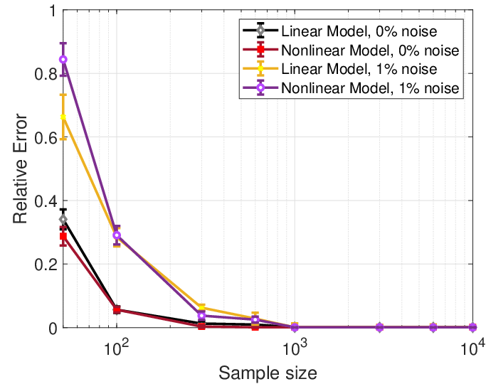
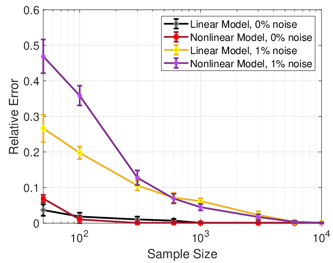
Fig. 6 shows the performance for the radial grid in Fig. 5 for linear and non-linear DC-PF voltages generated using simulated injection data. With noiseless data samples, the number of samples required for exact topology learning is approximately in either case. Perfect reconstruction under corrupted voltages with relative noise variance is observed at approximately samples. However, at samples, the average error is already below for both linear and non-linear models. While the performance improves with high sample sizes, note that the thresholds used for topology learning are not updated at each sample size, but fixed to the ones decided for asymptotically perfect recovery. In a realistic setting, the learning algorithm can consider the previous topology as a prior and select thresholds based on the pre-determined number of samples to improve the performance. Further the performance with linear and non-linear voltage samples are almost identical at sample sizes above . This follows from the acceptable accuracy of DC-PF in modeling the non-linear counterpart. Fig. 6 shows the performance of the algorithm for DC-PF for the loopy grid in Fig. 5. The performance, as expected, improves as the number of samples is increased. Beyond samples, the performance is comparable for linear and non-linear models under both noise and noiseless regimes.


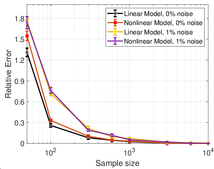
Next, we demonstrate the performance of Algorithm for AC-PF voltage samples , generated using the linear LC-PF Eq. (2), and the non-linear Matpower solver. The performance for the radial and loopy networks are given in Figs. 7 and 7 respectively. In the noiseless setting, average errors go down to zero for the radial case at samples, and for the loopy case at samples under both linear and non-linear models. With noise, the average errors are below for the radial case at samples, and below for the loopy case at samples. Perfect recovery in the noisy setting requires approximately samples in the radial case and samples in the loopy grid.
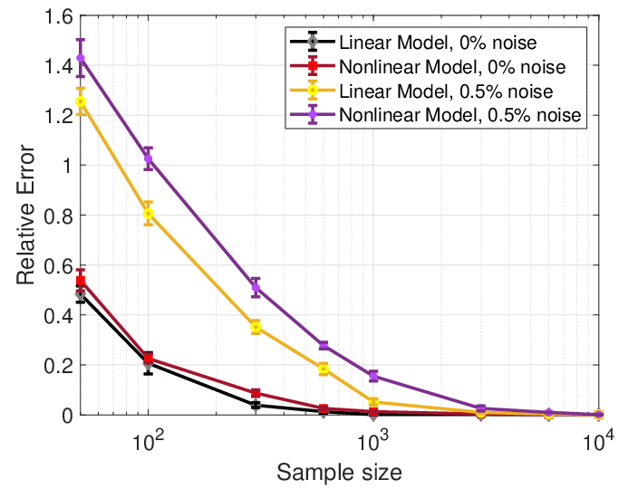
Finally, we present results using real power/active load data, sampled at minute intervals from real house-holds [29]. Fig. 8 demonstrates the performance of our learning algorithm for the loopy grid in Fig. 5, with linear and non-linear DC-PF samples. Note that the errors, in the noiseless setting, are below at samples for both the linear and non-linear case, despite no prior information about the topology. On the other hand, in the noisy setting, the average errors are below at samples. All the experiments have asymptotically correct recovery ( errors), which validates the theoretical consistency of our learning algorithm proven in the previous section.
 |
VI Conclusion
This paper discusses topology learning using nodal voltages in general power grids under a realistic regime: one where a subset of the internal nodes in the grid are unexcited and have zero injection. This regime makes the voltage covariance matrix degenerate, and standard inverse covariance or mutual information based learning methods do not apply. We provide a novel learning algorithm to overcome the presence of unknown zero-injection nodes, by first identifying them and their neighboring nodes, and then identifying the remaining edges in a Kron-reduced network without the zero-injection nodes. Using techniques from noisy regression and inverse covariance estimation, we prove the asymptotic correctness of our learning algorithm, both in the noiseless and noisy settings, when unexcited nodes are internal, non-adjacent and not present in loops of size . Notably, aside from voltage measurements, our algorithm does not use any prior information of structure, line parameters, values of nodal injections or their statistics. The theoretical contributions are validated by simulation results on IEEE test networks, with both linear and non-linear DC and AC voltage samples, corrupted with noise. Further, voltages generated using real injection data are used to caliberate the performance of our algorithm.
While our work focuses on power grids, it naturally extends to learning under-excited structured equation models that follow mass and flow conservation laws. Additionally, this article focuses on voltage samples collected from a static and balanced power flow model. Extensions to three-phase networks are possibly using voltage statistics proposed for the fully-excited setting [17]. Similarly, extending our work to learning power system and general dynamical systems [31, 32] in the under-excited regime, is another direction of future work.
References
- [1] D. Deka and et al., “Structure learning in power distribution networks,” IEEE Transactions on Control of Network Systems, 2018.
- [2] W. H. Kersting, “Radial distribution test feeders,” in Power Engineering Society Winter Meeting, 2001. IEEE, vol. 2. IEEE, 2001, pp. 908–912.
- [3] R. Hoffman, “Practical state estimation for electric distribution networks,” in Power Systems Conference and Exposition, 2006. PSCE’06. 2006 IEEE PES. IEEE, 2006, pp. 510–517.
- [4] R. Arghandeh and Y. Zhou, Big data application in power systems. Elsevier, 2017.
- [5] A. Phadke, “Synchronized phasor measurements in power systems,” IEEE Computer Applications in Power, vol. 6, no. 2, pp. 10–15, 1993.
- [6] A. von Meier and et al., “Micro-synchrophasors for distribution systems,” in Innovative Smart Grid Technologies Conference (ISGT), 2014 IEEE PES, 2014.
- [7] J. Peppanen and et al., “Increasing distribution system model accuracy with extensive deployment of smart meters,” in IEEE PES General Meeting, 2014.
- [8] S. Park and et al., “Exact topology and parameter estimation in distribution grids with minimal observability,” in PSCC, 2018.
- [9] G. Cavraro and V. Kekatos, “Graph algorithms for topology identification using power grid probing,” IEEE control systems letters, 2018.
- [10] G. Cavraro and V. Kekatos, “Inverter probing for power distribution network topology processing,” IEEE Transactions on Control of Network Systems, 2019.
- [11] C. Rudin and et al., “Machine learning for the new york city power grid,” IEEE Transactions on machine intelligence, 2011.
- [12] D. Wolter, M. Zdrallek, M. Stötzel, C. Schacherer, I. Mladenovic, and M. Biller, “Impact of meshed grid topologies on distribution grid planning and operation,” CIRED-Open Access Proceedings Journal, pp. 2338–2341, 2017.
- [13] J. Yu and et al., “Patopaem: A data-driven parameter and topology joint estimation framework for time-varying system in distribution grids,” IEEE Transactions on Power Systems, vol. 34, no. 3, 2018.
- [14] Y. Yuan, O. Ardakanian, S. Low, and C. Tomlin, “On the inverse power flow problem,” arXiv preprint arXiv:1610.06631, 2016.
- [15] M. He and J. Zhang, “A dependency graph approach for fault detection and localization towards secure smart grid,” IEEE Transactions on Smart Grid, vol. 2, no. 2, pp. 342–351, 2011.
- [16] S. Bolognani and et al., “Identification of power distribution network topology via voltage correlation analysis,” in IEEE Conference on Decision and Control (CDC), 2013.
- [17] D. Deka and et al., “Topology estimation using graphical models in multi-phase power distribution grids,” IEEE Transactions on Power System, 2019.
- [18] Y. Liao, Y. Weng, G. Liu, and R. Rajagopal, “Urban mv and lv distribution grid topology estimation via group lasso,” IEEE Transactions on Power Systems, 2018.
- [19] D. Deka, S. Talukdar, M. Chertkov, and M. Salapaka, “Graphical models in loopy distribution grids: Topology estimation, change detection and limitation,” IEEE Transactions on Smart Grid (early access), 2020.
- [20] K. A. Bollen, “Structural equation models,” Encyclopedia of biostatistics, vol. 7, 2005.
- [21] M. Baran and F. Wu, “Network reconfiguration in distribution systems for loss reduction,” IEEE Transactions on Power Delivery, 1989.
- [22] S. Bolognani and S. Zampieri, “On the existence and linear approximation of the power flow solution in power distribution networks,” Power Systems, IEEE Transactions on, vol. 31, no. 1, pp. 163–172, 2016.
- [23] Y. Dvorkin and et al., “Uncertainty sets for wind power generation,” IEEE Transactions on Power Systems, vol. 31, no. 4, pp. 3326–3327, 2016.
- [24] F. Dorfler and F. Bullo, “Kron reduction of graphs with applications to electrical networks,” IEEE Trans. on Circuits and Systems, 2013.
- [25] D. Deka, M.Chertkov, S. Talukdar, and M. V. Salapaka, “Topology estimation in bulk power grids: Theoretical guarantees and limits,” in Bulk Power Systems Dynamics and Control Symposium-IREP, 2017.
- [26] W. W. Hager, “Updating the inverse of a matrix,” SIAM review, 1989.
- [27] “IEEE 1547 Standard for Interconnecting Distributed Resources with Electric Power Systems.” [Online]. Available: http://grouper.ieee.org/
- [28] R. D. Zimmerman and et al., “Matpower 4.1 user’s manual,” 2011.
- [29] R. Pedersen, C. Sloth, G. B. Andresen, and R. Wisniewski, “Disc: A simulation framework for distribution system voltage control,” in 2015 European Control Conference (ECC). IEEE, 2015, pp. 1056–1063.
- [30] M. Grant and S. Boyd, “Cvx: Matlab software for disciplined convex programming, version 2.1,” 2014.
- [31] S. Talukdar and et al., “Learning exact topology of a loopy power grid from ambient dynamics,” in ACM e-Energy, 2017.
- [32] S. Talukdar and et al., “Physics informed topology learning in networks of linear dynamical systems,” Automatica, vol. 112, p. 108705, 2020.
-A Proof of Lemma 2
We decompose any as , where , and . We list two inequalities that we use in the proof.
| (25) | ||||
| (26) |
Consider with , , where is the optimal noiseless solution in Problem (9) for . Let denote the smallest non-zero singular value of . We have,
| (27) |
where follows from optimality of in the noiseless setting. denotes the projection of in the range of , and follows from Cauchy’s Interlace Theorem as is a principal sub-matrix of . By Eq. (12), for some . Then
| (28) |
Using the structure of and , we have, for ,
| (29) | ||||
| (30) | ||||
| (31) | ||||
| (32) |
Here follow from Eq. (25), and follow from Eqs. (28), (26). follows from the definition of in Eq. (17) and Eq. (26). Using Eqs. (30), (31), (32) in Eq. (29), we have
| (33) |
where and . Using the minimum value of quadratic functions, consider the cases for and their effect on .
| (a) | ||||
| (34) | ||||
| (b) | ||||
| (35) | ||||
| (c) | ||||
| (36) | ||||
| (d) | ||||
| (37) |
Using Eqs. (34), (35), (36), (37), . Using this in Eq. (27) completes the proof.
-B Proof of Theorem 5
Consider . From the proof of Theorem 1, note that zero-cost solutions in Problem (9) are given by , where .
, necessitates . Consider . Under the assumption in the statement, such that , but . Thus, , where follows from Eq. (8). As is non-positive for , holds only if . Following the same reasoning, , . Finally, is needed for . Thus, is the unique zero-cost solution for . It identifies the true neighbors of , due to the structure of .