SN 2019ehk: A Double-Peaked Ca-rich Transient with Luminous X-ray Emission and Shock-Ionized Spectral FeaturesFacilities: Hubble Space Telescope, Spitzer Space Telescope, Chandra X-ray Observatory, Neil Gehrels Swift Observatory, VLA, Las Campanas Observatory, Zwicky Transient Facility, Konkoly Observatory, ATLAS, Thacher Observatory, Swope:1m, Multi Unit Spectroscopic Explorer (MUSE), Shane (Kast), Xinglong Observatory (BFOSC), MMT (Binospec), Bok (B&C), Faulkes North (FLOYDS), NTT (EFOSC2), LJT (YFOSC), SOAR (Goodman, Triple-Spec), Keck I (LRIS)emcee (Foreman-Mackey et al. 2013), SNID (Blondin & Tonry 2007), Superfit (Howell et al. 2005), IRAF (Tody 1986, Tody 1993), AstroDrizzle (Gonzaga 2012), photpipe (Rest et al. 2005), DoPhot (Schechter et al. 1993), HOTPANTS (Becker 2015), Sedona (Kasen et al. 2006), SYN++/SYNAPPS (Thomas et al. 2011), Castro (Almgren et al. 2010), BPASS (Eldridge et al. 2017), MESA (Choi et al. 2016), sextractor (Bertin & Arnouts 1996), HEAsoft (v6.22; HEASARC 2014)
Abstract
We present panchromatic observations and modeling of the Calcium-rich supernova (SN) 2019ehk in the star-forming galaxy M100 (d16.2 Mpc) starting 10 hours after explosion and continuing for days. SN 2019ehk shows a double-peaked optical light curve peaking at and days. The first peak is coincident with luminous, rapidly decaying Swift-XRT discovered X-ray emission ( at days; ), and a Shane/Kast spectral detection of narrow H and He II emission lines () originating from pre-existent circumstellar material (CSM). We attribute this phenomenology to radiation from shock interaction with extended, dense material surrounding the progenitor star at and the resulting cooling emission. We calculate a total CSM mass of ( 6) with particle density . Radio observations indicate a significantly lower density at larger radii . The photometric and spectroscopic properties during the second light curve peak are consistent with those of Ca-rich transients (rise-time of days and a peak -band magnitude of mag). We find that SN 2019ehk synthesized of and ejected total with a kinetic energy . Finally, deep HST pre-explosion imaging at the SN site constrains the parameter space of viable stellar progenitors to massive stars in the lowest mass bin () in binaries that lost most of their He envelope or white dwarfs (WDs). The explosion and environment properties of SN 2019ehk further restrict the potential WD progenitor systems to low-mass hybrid HeCO WD + CO WD binaries.
Keywords:
supernovae:general — supernovae: individual (SN 2019ehk) — surveys — white dwarfs — X-raysI Introduction
Calcium-rich (Ca-rich) transients are a new class of faint, rapidly evolving astronomical transients that has been identified in the past two decades (Filippenko et al. 2003; Perets et al. 2010a; Kasliwal et al. 2012). Observationally, Ca-rich transients are characterized by peak magnitudes of to , rise-times days, and strong calcium features in photospheric and nebular phase spectra (Taubenberger 2017). The majority of these objects exhibit low ejecta and masses of and , respectively. Ca-rich transients do not necessarily have larger than average Ca mass but rather are “rich” in [Ca II] emission during the nebular phase. Consequently, Ca-rich spectra typically exhibit minimal [O I] emission and contain an integrated [Ca II]/[O I] flux ratio greater than 2.
The “Ca-rich” naming convention was reinforced by the Ca and O abundances of 0.135 and 0.037 derived from the nebular spectrum of prototypical event, SN 2005E (Perets et al. 2010a). However, subsequent modeling of Ca-rich transient nebular spectra using optical and near-infrared data highlight uncertainty in this estimate and suggest that chemical abundances may vary widely between events (Milisavljevic et al. 2017). A potential explanation for the prominence of Ca II emission relative to other species is that the distribution of 56Ni throughout the SN ejecta over-excites calcium ions (Polin et al. 2019a). Because of this, we choose to adopt the label suggested by Shen et al. 2019 and refer to these objects as “Calcium-Strong Transients” (CaSTs) from this point forward.
Early-time spectra of “gold sample” CaSTs (Shen et al. 2019) resemble that of core-collapse type Ib SNe (SNe Ib) with detectable photospheric He I and no observed H emission. However, the large fraction of objects found in old stellar environments on the outskirts of early-type galaxies disfavors a massive star origin for most CaSTs (Perets et al. 2011; Kasliwal et al. 2012). Parenthetically, CaSTs tend to occur in group or cluster environments of early-type elliptical galaxies with no evidence for local star formation or globular clusters (Perets et al. 2010a; Lyman et al. 2014; Foley 2015; Lunnan et al. 2017). Perets 2014 finds the location of CaSTs to be mostly consistent with older stellar populations, with many of these objects having large separations from early-type host galaxies known to have large stellar halos. Shen et al. 2019 also find that the radial distribution of CaSTs is consistent with old (¿5 Gyr), metal-poor stellar populations. However, a non-negligible fraction of CaSTs were found in disk-shaped galaxies (Perets et al. 2010a; Perets 2014; De et al. 2020).
A variety of progenitor scenarios have been proposed to explain the observed properties of CaSTs and their environments. Shen et al. 2019 outline the three scenarios that are most consistent with current observations. First, ultra-stripped-envelope SNe could reproduce the low ejecta and masses and rapidly evolving light curves, but cannot reconcile the lack of star formation at most CaST explosion sites. Similar discrepancies disfavor the second scenario wherein a WD is tidally disrupted by a neutron star (NS) or an intermediate-mass black hole (IMBH) (Rosswog et al. 2008; Metzger 2012; MacLeod et al. 2014; Sell et al. 2015; Margalit & Metzger 2016; Bobrick et al. 2017; Zenati et al. 2019b; Zenati et al. 2019a). While such a system is likely to occur in dense stellar systems like globular or super star clusters, there is currently no evidence for CaSTs occurring in such environments. However, SN kicks may push such systems outside of their typical cluster environments and still allow NS/BH + WD systems to reside at CaST explosion sites. Furthermore, NS+WD binaries occur at only 0.3-3% of the type Ia SN (SN Ia) rate for similar age populations, which is much less than the CaST rate of 10-94% with respect to SNe Ia (Perets et al. 2010a; Frohmaier et al. 2018; Toonen et al. 2018; De et al. 2020). Lastly, the detonation of a helium shell on the surface of a WD remains a viable option for CaSTs since its application in the study of SN 2005E (Perets et al. 2010a; Waldman et al. 2011; Woosley & Kasen 2011). In this case, the detonation of the He-shell could lead a partial second detonation of the C/O core for low mass WDs and still match the CaST observables. A complete second detonation of a near-Chandrasekhar mass WD would otherwise result in a SN Ia (Nomoto 1982; Woosley et al. 1986; Fink et al. 2010; Waldman et al. 2011; Polin et al. 2019b; Townsley et al. 2019; Perets et al. 2019; Zenati et al. 2019a). Given the proper conditions needed for helium shell detonations, this explosion scenario can successfully produce heightened Ca abundances through which the ejecta can effectively cool and subsequently produce the prominent Ca II emission lines seen in CaSTs (Holcomb et al. 2013; Polin et al. 2019a).
Despite attempts to find a singular progenitor scenario, some diversity is observed amongst SNe that display unusually large [Ca II]/[O I] flux ratios. This then suggests that CaSTs might be a heterogeneous class of objects with different physical origins. For example, the large inferred ejecta mass ( ) for iPTF15eqv is difficult to reconcile with other homogeneous properties of CaSTs (Milisavljevic et al. 2017). However, iPTF15eqv was only observed after optical peak, and its light curve is consistent with being more luminous than any of the known CaSTs. Together with its prominent H emission during nebular phase (also shown by the CaST PTF09dav, Sullivan et al. 2011), these findings might imply that iPTF15eqv is unrelated to the general sample of CaSTs, thus demonstrating the existence of different explosion channels responsible for Ca-rich emission at late times in SNe. An additional outlier amongst CaSTs is “Calcium-strong” SN 2016hnk (Galbany et al. 2019; Jacobson-Galan et al. 2019), which fits observationally within the class based on its peak luminosity, rise-time and [Ca II]/[O I] ratio, yet has a slowly decaying light curve as well as similarities to “SN 1991bg-like” SNe. This object may represent the extremes of the “Ca-rich” classification while still remaining consistent with the helium shell detonation scenario that is now considered to be a feasible explosion mechanism for CaSTs (De et al. 2020).
While the [Ca II]/[O I] flux ratio is the common metric for classifying new CaSTs, it is now clear that there is a substantial spread in this ratio amongst events: some objects such as SN 2003dg, PTF09dav and PTF10iuv have negligible [O I] emission, while SN 2012hn has an oxygen composition comparable to type IIb/IIP SNe (Valenti et al. 2014a, e.g.,). Furthermore, type Iax SNe (SNe Iax) are also thermonuclear explosions that are rich in [Ca II] emission at nebular times, yet do not belong to the typical CaST class (Foley et al. 2009; Foley et al. 2016).
Similar to other transients in the “thermonuclear zoo”, CaSTs have never been detected in X-ray observations (Sell et al. 2015; Milisavljevic et al. 2017; De et al. 2018; Sell et al. 2018; Prentice et al. 2019). The earliest X-ray follow-up of a CaST was at days after explosion by Sell et al. 2018 who was testing a progenitor scenario involving the tidal disruption of a WD by an IMBH for SN 2016hnk. However, the fact that multiple other studies have also found X-ray non-detections in CaSTs suggests that either (i) these objects resulted from progenitor environments where X-ray production is not possible or (ii) X-ray emission occurs in CaSTs at yet un-observed phases i.e., extremely early-times, days after explosion. Furthermore, no CaST has been detected in radio observations (Chomiuk et al. 2016). Progenitor mass-loss rates of and were derived from radio non-detections in iPTF15eqv and iPTF16hgs, respectively (Milisavljevic et al. 2017; De et al. 2018).
In this paper we present, analyze and model multi-wavelength observations (X-ray to radio) of a new CaST, SN 2019ehk, discovered by astronomer Joel Shepherd on 2019 April 29 (MJD 58602.24) using a TEC 140mm APO refracting telescope and Atik 460 EX Mono camera with an SDSS filter. SN 2019ehk has a discovery apparent magnitude of 17.1 mag and is located at , . The last non-detection of SN 2019ehk was on 2019 April 28 (MJD 58601.25), with a reported limiting -band apparent magnitude of mag. We fit a power law to the early-time data and derive a time of explosion of MJD .
We first classified SN 2019ehk as a young core-collapse SN with a blue, featureless continuum and strong Na I D absorption (Dimitriadis et al. 2019). Later observations of SN 2019ehk suggested a SN Ib classification with strong calcium features present in the photospheric spectra. However, the spectral time series of SN 2019ehk, coupled with its light curve evolution, indicated that it belonged to the CaST class.
SN 2019ehk is located 17.4′′ east and 13.9′′ north of the nucleus of the SAB(s)bc galaxy M100 (NGC 4321). In this paper, we use a redshift-independent host-galaxy distance of 16.2 Mpc reported by Folatelli et al. 2010, which is consistent with the Cepheid distance estimated by Freedman et al. 2001. However, it should be noted that there is a significant spread in reported distances for M100, which has influence on derived SN parameters. We use a redshift and standard CDM cosmology ( = 72 km s-1 Mpc-1, , ). The main parameters of SN 2019ehk and its host-galaxy are displayed in Table 1.
SN 2019ehk presents a remarkable opportunity to advance our understanding of this class of objects. Our observational coverage of this SN includes constraining pre-explosion Hubble Space Telescope (HST) imaging combined with a double-peaked light curve wherein the first peak is temporally consistent with luminous X-ray emission and “flash-ionized” Balmer series and He II spectral features. In §II we outline the reduction and analysis of archival HST, Spitzer and Chandra observations of the SN 2019ehk explosion site. In §III we describe all optical, IR, UV, radio and X-ray observations of SN 2019ehk. In §IV we present metallicity and star formation estimates for the explosion site in M100. In §V and §VI we present analysis and comparisons of SN 2019ehk’s optical photometric and spectroscopic properties, respectively, with chemical abundances of the SN and circumstellar medium derived spectroscopically in §VI.2 and §VI.3. In §VII we describe and model the first peak of the optical light curve of SN 2019ehk, while in §VIII we infer properties of the explosion’s immediate environment using X-ray and radio observations. Finally, in §IX we discuss the possible progenitor systems responsible for SN 2019ehk. Conclusions are drawn in §X. All uncertainties are quoted at the 68% confidence level (c.l.) unless otherwise stated.
II Pre-explosion observations and data analysis

II.1 HST observations
We analyze archival HST images of M100 from the Mikulski Archive for Space Telescopes (MAST) to search for the progenitor system of SN 2019ehk. These observations span from 31 December 1993 to 12 November 2009 and include a variety of filters on the Wide Field and Planetary Camera 2 (WFPC2) and the Wide Field Camera 3 (WFC3). Post-explosion Advanced Camera for Surveys (ACS) F814W imaging of SN 2019ehk was obtained under HST program PID-15645 (Sand 2018) on 23 May 2019. We follow the procedure outlined in Kilpatrick et al. 2018a to reduce all HST data with the astrodrizzle (Gonzaga 2012) reduction package.11 1 https://github.com/charliekilpatrick/hst123
We perform a fine alignment between pre- and post-explosion images in order to accurately look for a coincident progenitor source. For this we use the ACS F814W image of SN 2019ehk on 23 May 2019 and the deepest WFPC2 archival image in F555W taken on 7 January 1997. These specific images are presented in Figure 1 for reference. We first run sextractor (Bertin & Arnouts 1996) on both images to determine common sources to be used in the alignment process, with cuts made based on an individual sources’ full width at half maximum (FWHM) and relative flux. We find 220 common sources between pre- and post-explosion images.
We then performed image registration on the ACS image with IRAF22 2 IRAF, the Image Reduction and Analysis Facility, is distributed by the National Optical Astronomy Observatory, which is operated by the Association of Universities for Research in Astronomy (AURA) under cooperative agreement with the National Science Foundation (NSF). tasks ccmap and ccsetwcs. We used a fourth order polynomial in ccmap to fit pixel coordinates of all common sources in the WFPC2 image to the tangent plane projection of the right ascensions and declinations of the same sources in the ACS image. We then adjusted the WCS solution of the WFPC2 image with ccsetwcs. We calculate an astrometric uncertainty of and on the explosion site of SN 2019ehk in pre- and post-explosion images.
We apply the WCS solution from our fine alignment to all pre-explosion images and run dolphot to search for a source at the location of SN 2019ehk. We find no detectable source in any pre-explosion images within the uncertainty range of the relative astrometry. We then calculate 3 upper limits on a possible source coincident with SN 2019ehk by injecting fake stars and performing PSF photometry on these sources with dolphot. We present the upper limits in apparent magnitude (Vega system) for each pre-explosion HST filter in Table A1 and flux limits with respect to filter functions in Figure 26 of the Appendix.
All HST limiting magnitudes are used to constrain the luminosity and temperature of the SN 2019ehk stellar progenitor. First, we use pysynphot to generate a grid of luminosities ( L⊙) and temperatures ( K) assuming a blackbody stellar model. Each blackbody luminosity is normalized using the SN distance and uncertainty. For each luminosity and temperature in our grid, we convolve the associated spectrum with each HST filter in order to calculate the expected apparent magnitude. Then, in each filter, we cross-match the synthetic magnitude against the limit derived from fake star injection. If every synthetic magnitude is smaller than the pre-explosion limits then the luminosity/temperature grid point is rejected from the SN 2019ehk progenitor parameter space. We present the allowed/ruled out regions of pre-explosion parameter space (§IX.2) and discuss its implications for the progenitor of SN 2019ehk on the Hertzsprung-Russell diagram.
II.2 Spitzer observations
We perform a similar analysis of Spitzer pre-explosion imaging as in §II.1. We collect archival data of M100 from the Spitzer Heritage Archive that included multi-channel observations from 21 August 2014 to 12 April 2019 (Kasliwal et al. 2013; Kasliwal et al. 2014; Kasliwal et al. 2016; Kasliwal et al. 2018). For the fine alignment, we utilized explosion imaging of SN 2019ehk taken on 11 May 2019 under Spitzer program DD-14089 (Kasliwal et al. 2018). As in §II.1, we perform relative astrometry with IRAF and use dolphot to measure photometry of all detected sources. Upon inspection, we detect no pre-explosion source coincident with the location of SN 2019ehk. We then perform fake star injection with dolphot to estimate the limiting magnitudes of the SN 2019ehk progenitor. We report our 3 limits in the AB magnitude system in Table A2 and flux limits with respect to filter functions in Figure 26 of the Appendix. While the limits are not as constraining as those derived from HST imaging, we discuss implications of these observations in the context of dusty progenitors in §IX.2.
II.3 CXO observations
The Chandra X-ray Observatory (CXO) observed the location of SN 2019ehk with ACIS-S on multiple occasions between 1999 November 6 and 2012 February 16, for a total exposure time of 149.3 ks (observation IDs 400, 6727, 9121, 12696, 14230; PIs Garmire, Immler, Patnaude). We followed standard ACIS-S data reduction routines within CIAO v.4.12 employing the latest calibration files. Specifically, we reprocessed the data with chandra_repro and generated a merged event file from the individually re-projected files; this action also created a merged exposure map and a combined exposure map weighted PSF file. Running the source detection algorithm wavdetect on the merged event file using the exposure-map weighted PSF file we find no evidence for statistically significant X-ray emission from a point source at the location of SN 2019ehk. Adopting Poisson statistics we infer a 0.5-8 keV count-rate upper limit of ( c.l.), which translates into an unabsorbed flux limit in the range (0.3-10 keV) for a power-law spectrum with index , Galactic absorption (Kalberla et al. 2005), and intrinsic absorption . For a blackbody spectrum with keV and the flux limit is (0.3-10 keV).
III Post-explosion observations and data analysis
| Host Galaxy | M100 (NGC 4321) | ||||||||
| Galaxy Type | SAB(rs)c | ||||||||
| Galactic Offset | |||||||||
| Redshift | |||||||||
| Distance | Mpc33 3 Freedman et al. 2001; Folatelli et al. 2010 | ||||||||
| Distance Modulus, | mag | ||||||||
| Time of Explosion (MJD) | 58601.8 0.1 | ||||||||
| 0.02 0.001 mag | |||||||||
| 0.47 0.10 mag | |||||||||
| 0.34 0.14 mag44 4 Based on Balmer decrement of H II region at SN location. | |||||||||
| mag | |||||||||
| mag55 5 Extinction correction applied.66 6 Relative to second -band light curve peak | |||||||||
| m15 | magd |
III.1 UV/Optical photometry
We started observing SN 2019ehk with the Ultraviolet Optical Telescope (UVOT; Roming et al. 2005) onboard the Neil Gehrels Swift Observatory (Gehrels et al. 2004) on 1 May 2019 until 26 May 2019 ( 2.8 – 27.3 days since explosion). We performed aperture photometry with a 3′′ region with uvotsource within HEAsoft v6.26 (and corresponding calibration files), following the standard guidelines from Brown et al. 2014. We detect UV emission from the SN at the time of the first optical peak (Figure 2) until days after explosion. Subsequent non-detections in bands indicate significant cooling of the photosphere.
SN 2019ehk was imaged between 30 April 2019 and 1 August 2019 ( 1.2 – 94.2 days since explosion) with the Direct camera on the Swope 1-m telescope at Las Campanas Observatory, Chile and the PlaneWave CDK-700 0.7m telescope at Thacher Observatory in Ojai, California. Observations were performed in Johnson BV and Sloan ugriz filters. For these data, we performed bias-subtraction and flat-fielding, stitching, registration, and photometric calibration using photpipe (Rest et al. 2005). For our photometric calibration, we used stars in the PS1 DR1 catalog (Flewelling et al. 2016a) transformed from gri magnitudes to the uBVgri Swope natural system following the Supercal method (Scolnic et al. 2015). Difference imaging in gri bands was performed using PS1 templates. Final photometry was performed in the difference images with DoPhot (Schechter et al. 1993).
Las Cumbres Observatory (LCO) -band data of SN 2019ehk were obtained with the Sinistro cameras on the 1m telescopes at Sutherland (South Africa), CTIO (Chile), Siding Spring (Australia), and McDonald (USA), through the Global Supernova Project. Using lcogtsnpipe77 7 https://github.com/svalenti/lcogtsnpipe, a PyRAF-based photometric reduction pipeline, PSF fitting was performed. Reference images were obtained after the SN faded, and image subtraction was performed using PyZOGY (Guevel & Hosseinzadeh 2017), an implementation in Python of the subtraction algorithm described in Zackay et al. 2016. -band data were calibrated to Vega magnitudes (Stetson 2000) using standard fields observed on the same night by the same telescope. -band data were calibrated to AB magnitudes using the Sloan Digital Sky Survey (SDSS, Albareti et al. 2017).
SN 2019ehk was also observed with ATLAS, a twin 0.5m telescope system installed on Haleakala and Mauna Loa in the Hawai’ian islands that robotically surveys the sky in cyan (c) and orange (o) filters (Tonry et al. 2018a). The survey images are processed as described in Tonry et al. 2018a and photometrically and astrometrically calibrated immediately (Tonry et al. 2018b, using the RefCat2 catalogue;). Template generation, image subtraction procedures and identification of transient objects are described in Smith et al. 2020. Point-spread-function photometry is carried out on the difference images and all sources greater than 5 are recorded and all sources go through an automatic validation process that removes spurious objects (Smith et al. 2020). Photometry on the difference images (both forced and non-forced) is from automated point-spread-function fitting as documented in Tonry et al. 2018a. The photometry presented here are weighted averages of the nightly individual 30 sec exposures, carried out with forced photometry at the position of SN2019ehk. We searched for pre-explosion outbursts in archival ATLAS observations of the SN explosion site from MJD ( days before explosion). We assume Gaussian errors on the flux and test different phase-dependent binning combinations of pre-explosion data but do not find any photometric detections at ¿ 3 significance.
Additional follow-up photometry on SN 2019ehk was gathered at the Konkoly Observatory, Hungary, using the 0.8m RC80 telescope equipped with a FLI Proline 23042-1 back-illuminated CCD camera and filters. The frames are geometrically registered to a common pixel position then median-combined to create a deeper frame in each filter; transformation to the WCS was done by applying astrometry.net (Lang et al. 2010). Using IRAF tasks, image subtraction was applied using PS1 frames as templates, after pixel resampling, geometric registration, PSF- and flux-matching transformations of the template images. We then applied the publicly available Yoda code (Drory 2003) to get simple aperture photometry on both the SN and the local comparison stars. Transformation to the standard photometric system was done using the standard magnitudes of the local comparison stars from the PS1-catalog (Flewelling et al. 2016b). Uncertainties on the final magnitudes are computed by combining the photometric errors as given by Yoda and the residuals of the photometric zero points derived from the local comparison stars.
The Milky Way -band extinction and color excess along the SN line of site is mag and E(B-V) = 0.0227 mag (Schlegel et al. 1998; Schlafly & Finkbeiner 2011), respectively, which we correct for using a standard Fitzpatrick 1999 reddening law ( = 3.1). In order to estimate the effect of host galaxy extinction, we use a spectroscopic observation at the SN location from the Multi Unit Spectroscopic Explorer (MUSE), which observed M100 before the SN explosion on 28 April 2019 through ESO program PID 1100.B-0651 (PI Schinnerer). We apply a aperture (equal to the underlying H II region) to the MUSE data cube in order to extract a host spectrum. After accounting for the stellar absorption with Single Stellar Population (SSP) modeling within STARLIGHT (Cid Fernandes et al. 2005) as in Galbany et al. 2016, we measure a H and H line flux ratio of 4.23 and estimate the Balmer decrement through standard assumptions of Case B recombination (Osterbrock & Ferland 2006) and Fitzpatrick 1999 extinction law (). We derive a line of sight host galaxy reddening of mag.
In addition to the color excess derived from Balmer decrement in M100, there appears to be significant host galaxy extinction in the local SN environment. All photospheric spectra show prominent Na I D absorption with Equivalent Width EW 3 Å, at the host-galaxy redshift. We attempt to use Equation 9 in Poznanski et al. 2012 to convert the Na I EW to an intrinsic E(B-V), but the empirical relation shown in their Figure 9 becomes tenuous for EW 1.5 Å. Consequently, in order to derive an appropriate host extinction, we compare the r-i color to a sample of type Ic SNe (SNe Ic) (see §V.1). We find that E(B-V)=0.47 mag (corresponding to EW = 1.3 Å) is a reasonable estimate for host-galaxy extinction because it represents an average between the large extinction needed to match SNe Ic colors and a negligible extinction that is consistent with the observed color evolution in other CaSTs.
The complete light curve of SN 2019ehk is presented in Figure 2 and reference photometric observations are listed in Appendix Table A10. In addition to our observations, we include photometry from the Zwicky Transient Facility (ZTF; Bellm et al. 2019; Graham et al. 2019) public data stream. The most notable feature of the light curve is the presence of two peaks at days and days after explosion. Potential power sources of the first peak are presented in §VII while the luminosity of the later peak is considered to be derived from standard decay modeled in §V.2.
III.2 Optical/NIR spectroscopy
In Figures 3 and 4, we present the complete series of optical spectroscopic observations of SN 2019ehk from -12 to +257d relative to the second -band maximum ( days relative to explosion). A full log of spectroscopic observations is presented in Appendix Table A9.
SN 2019ehk was observed with Shane/Kast (Miller & Stone 1993), SOAR/Goodman (Clemens et al. 2004) and Keck/LRIS (Oke et al. 1995) between -12d and +257d relative to the second light curve peak. For all these spectroscopic observations, standard CCD processing and spectrum extraction were accomplished with IRAF. The data were extracted using the optimal algorithm of Horne 1986. Low-order polynomial fits to calibration-lamp spectra were used to establish the wavelength scale, and small adjustments derived from night-sky lines in the object frames were applied. We employed custom IDL routines to flux calibrate the data and remove telluric lines using the well-exposed continua of the spectrophotometric standard stars (Wade & Horne 1988; Foley et al. 2003). Details of these spectroscopic reduction techniques are described in Silverman et al. 2012.
SN 2019ehk was observed using EFOSC2 (Buzzoni et al. 1984) at the 3.58 m ESO New Technology Telescope (NTT) on 13 May 2019 through the ePESSTO+ program (Smartt et al. 2015; Nicholl et al. 2019). Grism #13 was used, with spectral coverage of 3500-9300 Å and resolution of 21 Å. The exposure time was 1500 s. Standard data reduction processes were performed using the PESSTO pipeline (Smartt et al. 2015)88 8 https://github.com/svalenti/pessto. The reduced spectrum was then extracted, and calibrated in wavelength and flux.
Las Cumbres Observatory (LCO) optical spectra were taken with the FLOYDS spectrographs mounted on the 2m Faulkes Telescope North and South at Haleakala (USA) and Siding Spring (Australia), respectively, through the Global Supernova Project. A slit was placed on the target at the parallactic angle. One-dimensional spectra were extracted, reduced, and calibrated following standard procedures using the FLOYDS pipeline99 9 https://github.com/svalenti/FLOYDS_pipeline (Valenti et al. 2014b).
One low resolution optical spectrum was taken with the 300 l/mm grating on the Boller & Chivens (B&C) spectrograph mounted on the 2.3m Bok telescope on Kitt Peak using a 1.5 arcsec slit width on 5 June 2019. Additionally, one moderate resolution spectrum was taken with the Binospec spectrograph (Fabricant et al. 2019) on the MMT using the 600 l/mm grating and 1” slit on 3 June 2019. Both the B&C and Binospec spectra were reduced using standard techniques in IRAF, including bias subtraction, flat-fielding, and sky subtraction. Flux calibration was done with spectrophotometric standard star observations taken on the same night at similar airmass.
The spectroscopic observations of SN 2019ehk were also collected using the Xinglong 2.16-m telescope (+BFOSC), and the Lijiang 2.4-m telescope (+YFOSC) (Fan et al. 2015) in China. The SN was observed between -11 to -7 days relative to second -band maxiumum. All the spectra were reduced using routine tasks within IRAF and the flux was calibrated with spectrophotometric standard stars observed on the same nights. Telluric lines are removed from all of these spectra whenever possible.
On 22 June 2019 (MJD 58656.0), we used the Triple-Spec instrument at SOAR to obtain a set of 3 ABBA observations of SN 2019ehk. We used the Spextool IDL package (Cushing et al. 2004) to reduce the Triple-Spec data, we subtracted consecutive AB pairs to remove the sky and the bias level, then we flat fielded the science frames dividing by the normalized master flat. We calibrated 2D science frames in wavelength by using comparison lamps obtained in the afternoon before the observations. To correct for telluric features and to flux calibrate our SN spectra, we observed the A0V telluric standard HD 111744 after the SN and at a similar airmass. Finally, we extracted the SN and the telluric star spectra from the 2D wavelength calibrated frames. After the extraction of the individual spectra, we used the xtellcorr task (Vacca et al. 2003) included in the Spextool IDL package (Cushing et al. 2004), to perform the telluric correction and the flux calibration of the spectra of SN 2019ehk. We combined individual observations of SN 2019ehk in a single spectrum shown in Figure 5.

III.3 X-ray observations with Swift-XRT and Chandra
The X-Ray Telescope (XRT, Burrows et al. 2005) on board the Swift spacecraft (Gehrels et al. 2004) started observing the field of SN 2019ehk on 01 May 2019, until 25 May 2019 ( d since explosion with a total exposure time of 11.4 ks, IDs 11337 and 11339). We analyzed the data using HEASoft v 6.22 and followed the prescriptions detailed in Margutti et al. 2013, applying standard filtering and screening. A bright source of X-ray emission is clearly detected with significance of against the background. Visual inspection reveals the presence of extended emission from the host galaxy at the location of the SN. Using Poisson statistics we find that X-ray emission from SN 2019ehk is detected with significance at d since explosion. No X-ray emission is detected above the host-galaxy level at later times.
We used Swift-XRT pre-explosion data acquired in 2005-2006 to estimate the level of emission from the host galaxy at the SN location (IDs 35227 and 30365). Merging all the available pre-explosion observations (exposure time of 59.1 ks), and extracting a spectrum from a 20′′ region centered at the SN location, we find that the host-galaxy emission is well modeled by a power-law spectrum with photon index , corresponding to a 0.3-10 keV unaborbed flux . The Galactic neutral hydrogen column density along our line of sight is (Kalberla et al. 2005). We use this model to account for the contribution of the host galaxy in the two post-explosion epochs where an excess of X-ray emission from SN 2019ehk is detected (at d and d).
For each of these two epochs we extracted a spectrum using a 20′′ region centered at the location of the SN. We find that the X-ray spectrum of the SN emission has a best-fitting photon index and for the first and second epoch, respectively, corresponding to an unabsorbed 0.3-10 keV flux of and . No evidence for intrinsic neutral hydrogen absorption is found ( at c.l. from the first epoch). We use the best-fitting spectral parameters inferred from the second epoch of observations to flux-calibrate the count-rate upper limits derived for the following epochs (Table A3). At the distance of SN 2019ehk these measurements indicate a steeply decaying, large X-ray luminosity with and at very early times d (Figure 7). The very luminous X-ray emission from SN 2019ehk at d rivals that of GRB 980425. Since no other CaST has been observed in the X-rays a few days since explosion, it is unclear if this luminous X-ray display is a common trait of the class.
The hard 0.3-10 keV X-ray spectrum of SN 2019ehk is suggestive of thermal bremsstrahlung emission with temperature keV. Fitting the SN contribution with a bremsstrahlung spectral model with keV the inferred emission measure is (at d) and (at d), where and are the number densities of electrons and ions, respectively.
The location of SN 2019ehk was serendipitously observed by the Chandra X-ray Observatory (CXO) on 15 February, 2020 ( d since explosion, exposure time of 9.95ks, ID 23140, PI Stroh) as part of follow-up observations of another supernova, SN 2020oi, that exploded in the same host galaxy. We analyzed the data with the CIAO software package v4.12 and corresponding calibration files. We find no evidence for X-ray emission at the location of SN 2019ehk and we place a 3 count-rate upper limit of (0.5-8 keV, pure Poisson statistics). We adopt the spectral parameters from the latest epoch of Swift-XRT observations that led to a detection and we infer an unabsorbed 0.3-10 keV flux limit , which corresponds to . This is the deepest limit on the late-time X-ray luminosity of a CaST to date (Figure 7).
III.4 Radio observations with the VLA
We acquired deep radio observations of SN 2019ehk with the Karl G. Jansky Very Large Array (VLA) at days post explosion through project VLA/19A-271 (PI D. Coppejans). All observations have been obtained at 6.05 GHz (C-band) with 2.048 GHz bandwidth in standard phase referencing mode, with 3C286 as a bandpass and flux-density calibrator and QSO J1224+21 (in A and B configuration) and QSO J1254+114 (in D configuration) as complex gain calibrators. The data have been calibrated using the VLA pipeline in the Common Astronomy Software Applications package (CASA, McMullin et al. 2007) v5.4.1 with additional flagging. Briggs weighting with a robust parameter of 2 was used to image. SN 2019ehk is not detected in our observations. We list the inferred flux densities in Appendix Table A4 and show how these measurements compare to radio observations of thermonuclear transients and core-collapse SNe in Figure 7(b).
IV Host Galaxy and Explosion Site
IV.1 Metallicity
We determine an oxygen abundance 12 + log(O/H) at the explosion site by using a MUSE spectroscopic observation taken on 28 April 2019 (PI Schinnerer). Data were reduced and analyzed following the prescriptions outlined in Galbany et al. 2016. The spectrum was corrected for a host galaxy reddening of mag and stellar absorption is accounted for with a SSP model (e.g., see §III.1). Using a combination of line flux ratios ([O III] / H and [N II]/H) into Equation 3 of Pettini & Pagel 2004, we determine a host metallicity of 12 + log(O/H) = dex ( Z⊙). We obtain a similar value if we use the method presented in Dopita et al. 2016: 12 + log(O/H) = dex ( Z⊙). The 0.3 dex difference between methods is expected given known offsets amongst calibrators (Kewley & Ellison 2008). Furthermore, both values are similar to the metallicities calculated by Pohlen et al. 2010 from the radial distribution of gas across M100.
IV.2 Star Formation Rate
We utilize the same pre-explosion MUSE spectrum to determine a star formation rate at the location of SN 2019ehk. We calculate a total H emission line luminosity of erg s-1 from a 0.7′′ aperture that encompasses the local H II region at the SN location. We then use Equation 2 from Kennicutt 1998 to estimate a star formation rate of SFR = yr-1 at the explosion site. We also derive an effective star formation rate of yr-1 kpc-2. These SFR values are reasonable considering the lack of observed star formation found at most CaST explosion sites. Our inferred rate is consistent with the low observed SFR values derived from of CaST explosion sites. With regards to core-collapse SNe, the H luminosity at the explosion site of SN 2019ehk is only consistent with the H II region luminosity at the location of of H-stripped SNe (e.g., Galbany et al. 2018; Kuncarayakti et al. 2018).
V Optical Light Curve Analysis
V.1 Photometric Properties
SN 2019ehk is the third observed CaST with a double-peaked optical light curve (the others being iPTF 16hgs, De et al. 2018 and SN 2018lqo, De et al. 2020). Consequently, we define its phase relative to the secondary, “Nickel-powered” peak and discuss the potential power sources of the first peak in §VII. We fit a low-order polynomial to the SN 2019ehk light curve to find best fit - and -band peak absolute magnitudes of mag at MJD and mag at MJD , respectively. We calculate a Phillips 1993 decline parameter value of mag from our -band light curve fits. We calculate a rise-time of days using the adopted times of explosion and -band peak.
We present and band light curve comparisons of SN 2019ehk and CaSTs in Figures 8(a)/(b). Overall, SN 2019ehk has comparable light curve evolution to other confirmed CaSTs: days and declines in luminosity at a similar rate. SN 2019ehk is less luminous in band than ”Calcium-strong” SNe 2016hnk (Galbany et al. 2019; Jacobson-Galan et al. 2019) and PTF09dav (Sullivan et al. 2011), but has a similar light curve evolution to the next most luminous CaST SN 2007ke (Lunnan et al. 2017). Furthermore, its band evolution is consistent with iPTF16hgs (De et al. 2018), the only other CaST with a confirmed double-peaked light curve. This duplicate first light curve peak may indicate similar underlying physics between the two objects despite the fact that SN 2019ehk is 1 mag more luminous than iPTF16hgs and declines at a slower rate. Additionally, we present vs. for SN 2019ehk with respect to CaSTs and other thermonuclear varieties in Figure 9. From this comparison, SN 2019ehk is broadly consistent with the CaST class due to its band light curve evolution from peak out to 15 days. SN 2019ehk is clearly distinct from normal and sub-luminous SNe Ia/Iax, but has a comparable Phillips 1993 decline parameter value to 91bg-like SNe Ia.
In Figure 10, we present , and color comparison plots of SN 2019ehk, CaSTs, SNe Ia/Iax and SNe Ic. Given the relative uncertainty on SN 2019ehk’s host-galaxy extinction, we display color curves that have no host extinction applied (red squares) as well as colors where the adopted value of mag is used to correct for extinction (blue line). As shown in Figures 10(a)/(c), SN 2019ehk’s de-reddened colors are consistent to within 0.1 mag in and 0.2 mag in of the typical CaSTs; all objects exhibiting a noticeably “red” color evolution. Consequently, SN 2019ehk’s intrinsically red colors deviate significantly from all flavors of SNe Ia shown in Figures 10(b). SN 2019ehk is 0.3 mag redder than the reddest SN Ia, 2005ke and SN Iax, 2012Z.
We present band light curve comparisons of SN 2019ehk and type IIb/Ib SNe (SNe IIb/Ib) in Figure 11(a). SN 2019ehk has a similar peak magnitude to SN Ib, iPTF13bvn and a higher peak magnitude than prototypical SN Ib, SN 2008D. While SN 2019ehk’s band evolution is quite similar to iPTF13bvn, it has a significantly shorter rise-time than any SNe Ib. With respect to SNe IIb, SN 2019ehk is less luminous at peak and evolves faster than both SNe 1993J and 2011dh. Furthermore, the first light curve peak observed in SNe IIb occurs on a longer timescale ( days) than that observed in SN 2019ehk (5 days). The first peak in these SNe is also typically less luminous than the secondary maximum, which is reversed in SN 2019ehk. However, the double-peaked light curve in SN 2019ehk may be physically connected to a explosion scenario wherein the SN shock “breaks out” into an extended envelope, which then rapidly cools. Such a mechanism has been invoked as an explanation for the primary peak in SNe IIb and we further discuss this model in §VII.3.
V.2 Pseudo-Bolometric Light Curve
We construct a pseudo-bolometric light curve by fitting the broad-band photometry with a blackbody model that is dependent on radius and temperature. Each spectral energy distribution (SED) was generated from the combination of multi-color optical photometry in bands (3000-9000Å). In regions without complete color information, we extrapolated between light curve data points using a low-order polynomial spline. We present SN 2019ehk’s bolometric light curve in addition to its blackbody radius and temperature evolution in Figure 12. We display the inferred blackbody luminosities, temperatures and radii that resulted from both host-galaxy extinction corrected photometry and non-corrected photometry. All uncertainties on blackbody radii and temperature were calculated using the co-variance matrix generated by the SED fits. It should be noted that the blackbody approximation breaks down when emission lines begin to dominate the spectrum of SN 2019ehk at days after explosion. Therefore a blackbody assumption for SN 2019ehk at late-times is most likely an over-simplification and could result in additional uncertainty on the presented bolometric luminosities and the resulting estimates on physical parameters of the SN. For the secondary, Nickel-powered light curve peak, we find a peak bolometric luminosity of .
In order to determine physical parameters of the explosion, we model the bolometric light curve with the analytic expressions presented in Appendix A of Valenti et al. 2008. We exclude the first light curve peak from this analysis and model the bolometric evolution of SN 2019ehk for days post-explosion. These models are divided into two distinct parts: the photospheric phase ( days past explosion), which is based on Arnett 1982 and the nebular phase ( days past explosion), which is derived from prescriptions outlined in Sutherland & Wheeler 1984 and Cappellaro et al. 1997 (however see Wheeler et al. 2015 for corrected Arnett 1982 equations). Furthermore, this analytic formalism self-consistently implements the possibility of incomplete -ray trapping in the expanding SN ejecta throughout the modeling process. A typical opacity of cm2 g-1 is applied in each model. The free parameters of each model are kinetic energy (), total mass of synthesized (), and ejecta mass (). However, there is a known degeneracy within these models between kinetic energy and ejecta mass:
| (1) |
where we follow standard practice and use , i.e. the photospheric velocity at peak. We use , which is estimated from Si II absorption at peak. Our photospheric and nebular models are presented in Figure 12(a) as the dashed and dotted lines, respectively. From these models, we calculate , erg and . We discuss the modeling of the first light curve peak in §VII.2. Furthermore, we show that the nebular phase light curve decline is slightly faster than the typical decay of that assumes complete trapping of -rays.
In Figure 12(b), we present the evolution of SN 2019ehk’s blackbody radius and temperature for different extinction values from 0.44 to 73.2 days after explosion. For phases 0.44-6d, it should be noted that the peak of the blackbody curve is not visible in our model fits i.e., the blackbody peaks in the near-to-far UV. Thus we cannot be confident that the reported blackbody radii and temperatures during these times are completely accurate. As is further discussed in §VII.1, these specific radii and temperatures are best treated as upper and lower limits, respectively.
At the time of first detection in band, SN 2019ehk had a minimum blackbody temperature of K and a maximum initial radius of cm (). This was conservatively calculated by assuming no color evolution between first and second epochs and then fitting a blackbody model. We can thus better constrain the initial radius at d by fitting a blackbody model to the initial band detection for a range of fiducial temperatures K. In this case we find photospheric radii of cm (1000-500 ). Extended progenitors for SN 2019ehk are ruled out in §IX.2. Therefore, considering a compact massive progenitor with radius of 10 , we estimate a shock velocity of in order to reach a blackbody radius of cm at d. This is also a reasonable estimate for shock breakout from a WD progenitor. Because the shock could be ahead of the photosphere, we consider to be a lower limit on the true shock velocity, which is consistent with being larger than the photospheric velocities derived from SN 2019ehk spectra.
VI Optical/NIR Spectral Analysis
VI.1 Spectroscopic Properties
We model the SN 2019ehk spectrum near peak in order to understand the chemical composition of the explosion. To do this, we utilize the spectral synthesis software SYNAPPS (Thomas et al. 2011), which is dependent on generalized assumptions about the SN such as spherical symmetry, local thermal equilibrium, and homologous expansion of ejecta. We present a SYNAPPS fit to the +1 day spectrum as the red line in Figure 13. As shown in blue, we detect the following species in SN 2019ehk near peak: He I, C II, O I, Na I, Mg I, Si II, S II, Ca II, Ti II, Fe II and Fe III. While the C II absorption is weak relative to the continuum, it does appear to be contributing to the overall flux near 6580,7234. The model also appears to be over-producing the line flux between 5500-6000Å, which we attribute to possible deficiency in fitting species such as S II, Ti II and Fe II. However, the overall spectral profiles are matches in that region, which allows us to conclude that those ions are in fact present in the SN ejecta.
We perform additional spectral modeling to explore the possibility that hydrogen or exotic Fe-group elements such as Cr II, Sc II and Sr II are present in SN 2019ehk. After multiple iterations of SYNAPPS modeling, we find no detectable H or Balmer series lines in the maximum light spectrum. Furthermore, the addition of Cr II, Sc II and Sr II to our SYNAPPS models does not improve the overall fit, specifically bluewards, and thus we cannot claim a confident detection of these ions. All identified ions in SN 2019ehk are typical of canonical CaSTs (e.g., 2005E-like) and indicate a similar chemical composition to be expected for an object within the class.
We track the expansion velocity of different ions through modeling of P-Cygni and pure emission line profiles. We estimate the photospheric velocities of various ions from first detection of spectral line formation at -9d to the last pre-nebular spectrum taken at +59d relative to the second band peak. At -9d, the fastest moving ions in the SN ejecta is Si II at and Ca II at ; this is measured from the fitted minimum of the absorption profile. These profiles, including O I and He I, show similar declines in velocity as the SN expands and becomes optically thin. We also measure Ca II and [Ca II] velocities from the FWHM of the and profiles, which remain approximately constant out to nebular times at and , respectively.
In the +38d NIR/IR spectrum of SN 2019ehk (Fig. 5), we identify similar ions to those found in our optical spectral modeling: He I, C I, Mg I and Ca II. We present the velocity profiles of He I in Figure 6. Both IR He I lines have identical P-Cygni line profiles, with showing a strong emission component and faster absorption minimum. The FWHM of the line is and the line is .
We present early-time spectral comparisons of SN 2019ehk and other CaSTs in Figure 14. Near (second) maximum light, SN 2019ehk is most similar visually to PTF12bho (Lunnan et al. 2017) and iPTF16hgs (De et al. 2018). All three objects have strong Ca II absorption, prominent He I profiles and the fast emergence of a [Ca II] profile relative to peak. SN 2019ehk and PTF12hbo both show little bluewards flux from Fe-group elements, which is unlike the prominent Fe-group transitions seen in iPTF16hgs, SN 2005E (Perets et al. 2010a) and PTF09dav (Sullivan et al. 2011). This may indicate either a low total Nickel mass (typical for these objects) or variation in the mixing of Fe-group elements in the outer layers of SN ejecta. This process can then result in the suppression of bluewards flux.
As shown in Figure 14(b), SN 2019ehk is nearly identical to SNe 2007ke and 2005E near +24 days after second maximum light. These pre-nebular spectra are dominated by [Ca II] and Ca II emission but are not yet optically thin given the observed P-Cygni profiles of He I and Ca II. Nonetheless, the prominence of [Ca II] emission at such an early phase indicates a rapid evolution towards the nebular regime and low enough ejecta densities to allow for efficient cooling through forbidden transitions. Furthermore, we compare nebular spectra of the majority of CaSTs to SN 2019ehk in Figure 15. Similar to all other CaSTs, there is no detectable emission from Fe-group elements in the bluewards spectrum; the majority of the observed flux being in [Ca II] emission, which shows no apparent [Ni II] line blending.

A common CaST classifier is a [Ca II]/[O I] line flux ratio greater than 2. We show the evolution of this ratio, in addition to a direct comparison of [O I] to [Ca II] lines in Figure 16. As seen in 16(a), even after reddening corrections, SN 2019ehk has the highest observed [Ca II]/[O I] ratio of any known CaST at days. This indicates that SN 2019ehk is not only more O-poor than most CaSTs, but it also has the fastest observed evolution to the optically thin regime. A quantitative discussion of elemental abundances in SN 2019ehk is presented in §VI.3.
While the spectral characteristics of SN 2019ehk appear to confidently place it within the CaST class, we explore the similarities between this SN and SNe Ib/IIb. As shown in Figure 11(b), SN 2019ehk, like other CaSTs, has similar spectral features to SNe Ib 2008D near peak such as detectable He I and Si II profiles and strong Ca II absorption. Compared to SNe IIb, the most apparent difference is the lack of a P-Cygni H and H profiles in SN 2019ehk, which only showed narrow H emission within 2 days of explosion. This suggests a H-rich CSM in SN 2019ehk while the broad H profiles in SNe IIb are indicative of H attached to an expanding photosphere. Finally, the line velocities in SN 2019ehk are slower overall than the photospheric velocities observed in SNe Ib and IIb: He I velocity is 6500 in SN 2019ehk, 9000 in iPTF13bvn and 7100 in SN 2011dh. These spectral differences may indicate that SN 2019ehk is the result of a different explosion scenario than these core-collapse SNe, but does not necessarily rule out a massive star progenitor.
VI.2 Inferences from “Flash-Ionized” H+He Spectral Lines at 3 days
The earliest spectrum obtained -11.9 days before second -band maximum (1.45d since explosion) shows narrow H and He II 4686 emission lines with width of 500 . The observed velocities are greater than the spectral resolution of the Kast spectrograph () used to detect this spectral features. These lines are partially detected in the spectrum acquired on day -11.1, but not on day -10.8 (2.3 and 2.6 days since explosion, respectively) (Figure 17). Furthermore, we visually identify potential narrow He I emission near in the earliest spectrum with a 1 detection confidence. We present its velocity profile for reference in Figure 17 and note that, if real, the species is below the 3 detection threshold. Accounting for the brightening of the underlying continuum we conclude that there is evidence for fading of H and He II line flux by a factor 2 at 3 c.l. between the second and third epoch. These emission profiles are similar to those found in young core-collapse SNe and are thought to form from “flash” or shock-ionized CSM surrounding the progenitor star (Gal-Yam et al. 2014; Kochanek 2019).
The line width of 500 (Figure 17), significantly lower than the velocity of material in the explosion’s photosphere (§VI.1), indicates that the emission arises from CSM produced via mass-loss before the explosion (as opposed to originating in the explosion’s ejecta). The detection of H and He emission lines with these properties thus establishes the presence of H and He-rich CSM around SN 2019ehk. The time of their disappearance and relative luminosity enable inferences on the location of the CSM and its chemical composition, as we detail below.
The H and He II 4686 luminosities of and , respectively, measured at 1.45 days since explosion imply assuming Case B recombination (Hummer & Storey 1987). The luminosity limit of the He I 7065 line can be used to infer an upper limit on the amount of He+ using recombination rates from Benjamin et al. 1999, so that we find
| (2) |
implying partial burning of hydrogen.
The SN shock break out radiation cannot be responsible for the ionization of the CSM at days, as the recombination timescale for H+ and He++ is and a few hours for gas temperatures K and free electron densities (e.g. Lundqvist & Fransson 1996). The source of ionizing radiation can be provided by the luminous X-ray emission (Fig. 7) that resulted from the SN shock interaction with the CSM (§VIII.1). In this scenario the fading of the H and He recombination lines is related to the time when the SN shock overtakes the CSM shell. We infer an outer CSM shell radius cm, for the SN shock to reach it in 2 days (for a typical shock velocity 0.1c), and an emission measure to account for the observed recombination line luminosities at 1.45 days after explosion. From these inferences we derive a CSM density1010 10 Note that this is the density of the unshocked CSM gas illuminated and ionized by the X-ray emission from the SN shock. and a CSM shell mass of assuming a spherical shell (cm) and unity filling factor. Note that the filling factor cannot be less than about 0.3 without reducing the ionization parameter to less than 30 and producing too much He I emission. Based on the abundance by number shown in Eqn. 2, we estimate a CSM H mass in the range and a He mass of .
We end by noting that for these physical parameters, the resulting ionization parameter (where is supplied by the X-ray luminosity) has values intermediate between those needed to doubly ionize helium (as observed), but lower than those necessary to produce high ionization lines such as [Fe X], which are not seen in the spectra of SN 2019ehk (but detected in other SNe with CSM interaction, e.g., SN2014C, Milisavljevic et al. 2015).
VI.3 Inferences from Nebular Phase Spectroscopy at 30 days
Table 2 lists the emission line luminosities measured from spectra acquired on 31, 38 and 59 days since second -band maximum. Recombination lines of He I, C I, O I and Mg I are detected, along with forbidden lines of [O I] and [Ca II] and permitted lines of Ca II, while we consider the possible H feature to be an upper limit. Uncertainties in the underlying continuum and the wavelength ranges of some of the lines cause up to factor of 2 errors in the inferred luminosities, especially for lines that show prominent P-Cygni profiles. With this caveat in mind, we find that the ratios of He I line fluxes approximately agree with those predicted with the atomic rates of Benjamin et al. 1999 for densities up to at a temperature of K.
The inferred blackbody radius at 59 days after second -band maximum (72 days since explosion) is cm (Figure 12). The maximum velocity shift of the [Ca II] emission feature is 5000 , corresponding to a radius of cm. The nebular emission is produced between those radii, so we take the volume to be about . The observed He I line luminosities and inferred volume require at 59 days since second B-maximum. We note that the He I 7065 line is stronger than expected, probably because of repeated scatterings that convert He I 3889 photons into emission at 7065. This scenario is supported by the prominent P-Cygni profiles of the He I NIR lines, which indicate large optical depths and a substantial population of the 1s2s 3S metastable level.
The relative luminosities and recombination rates from Hummer & Storey 1987 and Julienne et al. 1974 imply number density ratios and = 1.5. If no other elements contribute significant numbers of free electrons, the densities of electrons, He+, H+ and O+ are 3.8, 1.0, 1.3 and , respectively. If carbon contributes free electrons, will be correspondingly higher and the densities of the ions correspondingly lower. The limit on the ratio of He+ to H+ is similar to the He/H ratio derived for the CSM (§VI.2), so H:He:O ratio may be similar to the values above.
At densities above , the [O I] and [Ca II] lines are in their high density limits, and their luminosities are given by the populations of the excited states multiplied by the Einstein A values:
| (3) |
| (4) |
where h is the photon energy, the exponentials are the Boltzmann factors ( is in K) and the numerical factors are statistical weights. The observed luminosities of the [Ca II] lines are much higher than the [O I] luminosities ( at 257 days since second -band maximum, Figure 16). From Eqn. 3-4:
| (5) |
where we used K, and . We thus infer . Since there is a strong overlap of the temperature and ionization parameter ranges where O I and Ca II exist, we expect , implying that, as in iPTF15eqv (Milisavljevic et al. 2017), the prominent Ca lines result from the density and ionization state of the ejecta rather than an overabundance of Ca with respect to O. We note that the [O I] and [Ca II] lines are likely to arise from a region of lower electron density than the recombination lines, because the forbidden lines are strongly suppressed at densities above , leading to higher ratios of the 8600 calcium triplet to the [Ca II] lines than are observed. The Ca II feature at 11873 is much stronger than expected for optically thin emission, even if the 4s-5p lines from the ground state are converted to 11873 through multiple scatterings. It is possible that the He II 1640 line pumps the 4s-5p transition, since the separation is about 1700. If so, the He II line is formed by recombination, and this would be the only indication of doubly ionized helium in the nebular gas.
Assuming temperatures of 104 K for the recombination lines and 5000 K for the forbidden lines, the densities and volume yield rough mass estimates from the day +59 spectrum (from second -band max) of 0.008, 0.037, 0.10 and 0.004 for He+, O+, O0 and Ca+, respectively. It should be noted that at these phases the SN is not fully nebular and therefore the derived masses may be lower than the true elemental masses in the explosion.
| Wavelength | Line ID | Day +31 | Day +38 | Day +59 |
|---|---|---|---|---|
| (Å) | () | () | () | |
| 5876 | He I | 17 | – | 2.3 |
| 6303,6363 | [O I] | 19 | – | 7.3 |
| 7065 | He I | 14 | – | 4.5 |
| 7291,7324 | [Ca II] | 220 | – | 130 |
| 7774 | O I | 18 | – | 4.9 |
| 8579 | Ca II | 290 | – | 150 |
| 9224 | O I | 21 | – | 5.0 |
| 10830 | He I | 94 | 162 | 29. |
| 11873 | Ca II | – | 72 | |
| 14878 | Mg I | – | 14 | |
| 15900 | C I | – | 16 | |
| 20589 | He I | – | 16 |
Note. — No extinction corrections have been applied to the presented apparent magnitudes.
Note. — In our latest spectrum at +257d, [Ca II] and [O I] luminosities are erg s-1 and erg s-1, respectively.
VII The optical “Flare”
Here we describe the observational properties of the first light curve peak and present physical models that can explain this initial increase in total flux. In an effort to be succinct, we hereafter refer to this primary light curve evolution as the “flare.” In this section, all times are referred with respect to the explosion.
VII.1 Observational Properties
The flare is observed across all UV, optical and NIR photometric bands from the first band detection at 0.44 days until 7 days after explosion. We present SN 2019ehk’s color, photometric and spectral evolution during the flare in Figure 18. We observe an initial rise in band flux from 0.44-1.38 days and then seemingly constant flux between 1.38 and 2.81 days. However, in some photometric bands (e.g., ) the flux in this phase range appears to be decreasing. This indicates that there could be 2 separate peaks within the flare or possibly separate emission mechanisms at these early-times. Then, as shown in Figure 18(b), the most dramatic flux increase occurs in day and peaks at days. This is reflected by a 1 mag flux increase in all photometric bands. During the early rise, the flare spectrum is blue and mostly featureless, with transient H and He recombination lines that soon subside (§VI.2). Clear photospheric spectral features (e.g., Si II, O I, Ca II) first appear after the flare’s peak at days after explosion (Figure 18c).
We present SN 2019ehk’s blackbody radius , temperature and resulting bolometric luminosity evolution during the flare in Figure 19 (shown as squares). As discussed in §V.2, at days the blackbody SED peak lies in the mid-UV, outside the range covered by our complete photometric dataset. At these times the data provide lower limits on the blackbody temperature and upper limits on the radius, which results in a lower limit on the true bolometric luminosity (arrows in Figure 19). The bolometric light curve at days was likely dominated by UV radiation and decreased rapidly from a peak luminosity potentially larger than erg s-1 shown in Figure 19 with red squares.
A reasonable assumption for stellar explosions at early times is that of a photosphere expanding homologously in time (e.g., Liu et al. 2018). Here we make the simplistic assumption of a linear evolution of the photospheric radius with time, , where we take , similar to the velocities observed in the first photospheric spectra and is the initial envelope radius (black dotted line in Fig. 19, lower panel). Interestingly, the resulting matches the photospheric radius at days. Freezing the blackbody radius to the values implied by the linear evolution with time in our blackbody fits leads to larger inferred temperatures, as expected (Fig. 19, middle panel). The resulting bolometric luminosity is also consequently larger (Fig. 19, upper panel). While we consider these estimates to lead to a more realistic bolometric output at early times, we caution that the assumption of a linearly increasing photospheric radius is likely an over-simplification and that accelerated expansion could have a significant influence on the very early-time SN evolution.
VII.2 Nickel Powered Model
A possible power source for the flare emission is the radioactive decay of an amount of that was heavily mixed into the outer layers of ejecta. This mass is distinct from the centrally located that is responsible for the main SN optical peak. As discussed in De et al. 2018 for iPTF16hgs, this distribution of could result in two distinct light curve peaks, each powered by its own supply of 56Ni (e.g., see also Drout et al. 2016). We test the validity of this model for SN 2019ehk by applying the same analytic model for a radioactively powered light curve as that presented in §V.2. We find ergs and . A total ejecta mass of is estimated using , which is derived from Si II absorption near the peak of the flare.
This model both produces a poor fit to the flare’s bolometric luminosity as well as results in a ratio greater than 1, which is clearly unphysical. Furthermore, this model is disfavored because it does not naturally explain the presence of early-time X-ray emission. If an exterior plume of 56Ni is the power-source behind the flare, an additional, independent ingredient would need to be invoked to explain the X-rays, which would have occurred coincidentally at the same time as the optical flare, but would otherwise have no physical connection to the flare. More natural scenarios are those where the optical flare and the X-ray emission are different manifestations in the electromagnetic spectrum of the same physical process (§VII.3, §VII.4).
VII.3 Shock Breakout and Envelope Cooling Model
It is now understood that shock breakout through an extended distribution of material (e.g., stellar envelope) can increase the SN flux above the typical radioactively powered continuum emission. The resulting observational signature is a double-peaked light curve where the first peak originates from the expansion and cooling of the shocked envelope, followed by the standard SN peak of emission. This is typically observed in SNe IIb (e.g., SNe 1993J, 2011dh and 2016gkg; Wheeler et al. 1993; Arcavi et al. 2011; Arcavi et al. 2017; Piro et al. 2017) and numerous models have been put forward to explain this observational signature with breakout and cooling emission into an expanding envelope (Nakar & Piro 2014; Piro 2015; Sapir & Waxman 2017).
As discussed in §VII.1, the light curve exhibits nearly constant flux at days before the dramatic rise and decline in magnitude from days. Furthermore, as illustrated by the magenta and grey dotted lines in Figure 20, H and He emission lines persist in SN 2019ehk spectra until days and fade in visibility when the primary peak of the flare occurs at days. These observational signatures suggest separate emission components within the flare: one that allows for H + He spectral emission in addition to unremitting flux ( days), and one that induces a substantial rise in flux without “flash-ionized” spectral lines ( days). Consequently, we choose to model each of the observationally distinct regimes within the flare separately.
In the following sections, we describe and apply three models for a shock cooling emission mechanism to explain the entire evolution of the optical flare in SN 2019ehk. At the time of explosion, each model produces constraints on the envelope mass, , envelope radius, , the velocity of the shock or envelope, and the time offset from explosion (consistent with our explosion time estimate). In this analysis, we use emcee, a Python-based application of an affine invariant MCMC with an ensemble sampler (Foreman-Mackey et al. 2013). We compile the best fit parameter estimates from each model in Table A5. While in §VII.3 we model the flare emission with two cooling-envelope components, we note that the presence of H and He emission in the first flare component requires a persistent source of ionizing radiation that might not be provided by pure cooling-envelope models, which motivates our investigation of models that also include ongoing CSM interaction in §VII.4
VII.3.1 Nakar & Piro 2014 Model
Nakar & Piro 2014 present scaling relations for “non-standard” core-collapse SN progenitors with compact cores surrounded by extended envelopes. By showing that the peak of the optical flux will occur when the mass depth (i.e., photon diffusion distance within mass) is equal to the envelope mass (), they construct the following analytic expression for :
| (6) |
where is the expansion velocity of the extended envelope, is the time to first light curve peak and the opacity is cm2 g-1. As discussed in §VII.3, it is likely that the flare is the product of separate emission mechanisms, each occurring on different timescales. As a result, we apply the Nakar & Piro 2014 model to each “peak” within the flare at times and days. We estimate an envelope velocity of cm s-1 from the absorption minimum of the He I transition, which is the first detectable spectral feature to appear at days after explosion.
Furthermore, from Nakar & Piro 2014, the envelope radius can be expressed as:
| (7) |
where erg s-1. At days and days, we calculate peak bolometric luminosities of and erg s-1, respectively. They also predict the observed temperature at as:
| (8) |
Using this expression for and , we calculate observed flare temperatures of and K, respectively; both of which are consistent with derived blackbody temperatures at the same phase as shown in Figure 19. Overall, we caution against the accuracy of these model outputs due to uncertainties surrounding the bolometric luminosities at days. As discussed in §V.2, we can only place solid constraints on upper and lower limits on the blackbody radii and temperature during the flare, which then affect the bolometric luminosity at those times. Thus the and values derived from the Nakar & Piro 2014 models should be treated as lower limits given the uncertainty on each peak luminosity. For the main peak of the flare and opacity cm2 g-1, we estimate an envelope mass of and radius of 100 .
VII.3.2 Piro 2015 Model
Starting from the scaling relations at from Nakar & Piro 2014, Piro 2015 presents a generalized analytic model that allows a direct, detailed comparison to the observed flux evolution with time. The SN shock is assumed to propagate into extended material of mass of unknown chemical composition surrounding the progenitor star core with mass . This is a one-zone model that does not include a prescription for the density profile, gradient or chemical composition of the extended material. Following Piro 2015 the expansion velocity and the energy passed into the extended material read:
| (9) |
| (10) |
where erg. Piro 2015 show that the shocked extended material will expand (with characteristic radius ) and cool, with an observed peak of emission occurring at time :
| (11) |
In their Eqn. 15, Piro 2015 present a predicted bolometric luminosity from shock cooling as:
| (12) |
where .
Following Arcavi et al. 2017 and Piro 2015, we model the emission from the extended mass as a blackbody spectrum with radius and temperature:
| (13) |
We calculate the expected apparent magnitudes for individual photometric bands from this model using the pysynphot Python package and we fit these models to the (extinction-corrected) apparent magnitudes of SN 2019ehk in bands at days. As before, we fit the data at d and days as two separate components. For all models we adopt erg, cm2 g-1 and (§V.2). It should be noted that the chosen core mass has little impact on the final inferred parameters. We present all multi-color light curve fits using these models as the solid lines in Figure 20. As shown in the plot, this simplified model provides a reasonable match to the data for both components of the flare. The best fitting values for both components are reported in Table A5.
VII.3.3 Sapir & Waxman 2017 Model
Sapir & Waxman 2017 present an updated version of the model by Rabinak & Waxman 2011, which applies to the immediate post-shock breakout evolution at few days, when the emission is dominated by radiation from the external envelope layers, and extends the solutions by Rabinak & Waxman 2011 to later times, when the observed emission originates from the inner envelope layers and depends on the progenitor density profile. Sapir & Waxman 2017 adopt a progenitor structure with a polytropic hydrogen-dominated envelope, which they demonstrate numerically can power an initial light curve peak through shock cooling.
Below we present the analytic expression for the envelope’s bolometric luminosity that was derived by Arcavi et al. 2017 starting from Sapir & Waxman 2017:
| (14) | |||
where cm, cm s-1, and is in days. This model is for a polytropic index of , which encompasses both stars with convective envelopes as well as radiative envelopes e.g., RSGs[BSGs], respectively. Same as for the Piro 2015 models, we adopt . The dimensionless scaling factor from Sapir & Waxman 2017 is:
| (15) |
Finally, Arcavi et al. 2017 present an envelope temperature derived by Sapir & Waxman 2017 to be:
| (16) | |||
We assume a blackbody spectrum and perform the same analysis as in §VII.3.2 to extract apparent magnitudes from the predicted luminosity and temperature. We model the flare by the same methods and present light curve fits for an and polytropes as solid and dashed lines, respectively, in Figure 20. We find that the first flare component at d can be fit accurately with our MCMC model. For the first peak within the flare, we estimate envelope radii and masses of and for n = 3[3/2] polytropes. The MCMC routine, however, does not formally converge when we attempt to fit the entire data set at d. In Figure 20 we show a representative model, with parameter values indicated in Table A5. These values should be treated as order of magnitude estimates.
We end by noting that the model by Sapir & Waxman 2017 is valid for times:
| (17) |
| (18) |
We test the validity of our derived model parameters (Table A5) with Equations 17 and 18 and we find that our model parameters satisfy the relations above. For the first peak in the flare we find: days (n = 3/2) and days (n = 3). For the second peak we find: days (n = 3/2) and days (n = 3). All derived timescales are valid for the duration of the flare.
In the previous three subsections we have investigated a shock cooling model as a power source for the flare. Because of its temporal structure, we have modeled the flare in two components ( and days) in order to derive physical parameters (e.g., radius, mass, velocity) of a shock heated envelope needed to match optical the optical light curve. Figure 20 demonstrates that modeling the entire flare with one shock cooling model cannot reproduce the observations but the corresponding radii and masses for each model represent upper limits on the total amount of shocked material capable of powering the flare.
VII.4 CSM Interaction Model
Another potential source of energy to power the optical flare emission is via ongoing SN shock interaction with the medium. This scenario has physical similarities to that discussed in §VII.3 with the key difference being that rather than powering this rapid light curve peak via post-breakout cooling emission, the CSM interaction model allows for continuous energy injection due to the ongoing conversion of shock kinetic energy into radiation. The presence of CSM around the SN 2019ehk progenitor is evident given the detection of flash-ionized H and He features in the first optical spectrum at 1.45 days since explosion. The estimated blackbody radius at the time of the first spectrum is cm (§V.2) and the velocities of H- and He-rich material are and , respectively (§VI.2). The flash-ionized CSM lies in front of the photosphere at radii cm. Therefore, this H+He rich material was lost by the stellar progenitor to the environment 3 months prior to explosion.
We quantitatively test the scenario of a SN shock interacting with a shell of CSM through 1D numerical radiation hydrodynamics simulations with the CASTRO code (Almgren et al. 2010). Equations for radiation hydrodynamics are solved using a gray flux-limited non-equilibrium diffusion approximation. The models are similar to those applied to the SN Ic-BL, 2018gep (Ho et al. 2019) and the fast-evolving luminous transient KSN 2015K (Rest et al. 2018), but have been adapted to the observables in SN 2019ehk.
Our simulations assume spherical symmetry wherein the SN ejecta expands homologously and is characterized by a broken power-law density profile (, with ), ejecta mass , energy , initial outer radius , outer velocity and ejecta temperature K. The CSM shell is assumed to have constant density and is initialized with temperature K. We adopt a static CSM (i.e. ) whose velocity has no affect on the model results so long as . The shell is described physically by its mass , radius and thickness . Once the ejecta have reached homology we use the radiative transfer code Sedona (Kasen et al. 2006) to generate synthetic bolometric light curves as well as the temporal evolution of the effective blackbody temperature and radius in each model. Unlike other CSM interaction codes (e.g., MOSFIT, Guillochon et al. 2018; TigerFit, Chatzopoulos et al. 2016) that use the semi-analytic Arnett approximation with a parameterized heating term, our simulations self-consistently solve for the time-dependent light curves by evolving the coupled radiation hydrodynamics equations with CASTRO.
From a grid of shock interaction simulations, we find that the first component of the flare is best fit by shock breakout emission into a CSM characterized by the following parameters: mass , radius cm, thickness cm and opacity cm2 g-1. This model was initialized for a SN with , which is based on observations as constrained by our modeling of §V.2. This model is presented with respect to SN 2019ehk’s bolometric luminosity, temperature and radius evolution during the flare in Figure 19. We also show a CSM interaction model that is able to power the entire flare (d) with and the same physical parameters as above. These CSM properties are consistent with the masses independently inferred from the optical spectral modeling of §VI.2 and X-ray modeling of §VIII.1.
VIII Radio/X-ray data Modeling
VIII.1 Inferences on the explosion’s local environment from X-ray observations
The luminous (), rapidly-decaying X-ray emission () with a hard spectrum is consistent with thermal bremsstrahlung from shocked CSM gas in adiabatic expansion. In this scenario the X-ray luminosity scales as the emission measure , and once the shock has swept up most of the CSM gas. For , the measured from the first epoch of X-ray observations at d indicates a particle density , where and are the radius and thickness of the shocked shell of gas in units of , respectively, and is a volume filling factor. This density estimate is remarkably similar to the density of the pre-shocked CSM gas that we have inferred from the H and He recombination lines (§VI.2). The inferred mass of the shocked gas is .
For a typical SN shock velocity of , the forward shock radius at d is . The disappearance of the H and He recombination lines by d post explosion and the rapid fading of the X-ray luminosity detected at 2.8 d indicate that the shock has overtaken the shell of CSM by this time. Using and assuming we infer a particle density of and a total CSM shell mass of (for ). This result is consistent with the mass of pre-shocked CSM gas that was in front of the shock at d since explosion derived in §VI.2. Together with the modeling of the flare optical continuum of §VII, these results strengthen the scenario where the detected X-rays and continuum optical emission originate from pre-existing H/He rich CSM shocked by the SN blastwave, while the H and He recombination lines result from pre-shocked CSM gas lying in front of the SN shock and ionized by its X-ray emission. If the chemical composition of the entire shell is similar to that constrained by the H+He emission lines of §VI.2, and under the assumption of , the total CSM H mass is in the range and the total CSM He mass is constrained within the range .
VIII.2 Inferences on the explosion’s environment at from radio observations
We interpret the radio upper limits of §III.4 in the context of synchrotron emission from electrons accelerated to relativistic speeds at the explosion’s forward shock, as the SN shock expands into the medium. We adopt the synchrotron self-absorption (SSA) formalism by Chevalier 1998 and we self-consistently account for free-free absorption (FFA) following Weiler et al. 2002. For the calculation of the free-free optical depth we adopt a wind-like density profile in front of the shock, and we conservatively assume a gas temperature (higher gas temperatures would lead to tighter density constraints). The resulting SSA+FFA synchrotron spectral energy distribution depends on the radius of the emitting region, the magnetic field, the environment density and on the shock microphysical parameters and (i.e. the fraction of post-shock energy density in magnetic fields and relativistic electrons, respectively).


Figure 21 shows the part of the density vs. shock velocity parameter space that is ruled out by the upper limits on the radio emission from SN 2019ehk for three choices of microphysical parameters. Specifically, we show the results for and (which have been widely used in the SN literature) to allow a direct comparison with other SNe (black dots in Figure 21). We find that SN 2019ehk shows a combination of lower environment density and lower shock velocity when compared to core-collapse SNe with radio detections. As a final step, we self-consistently solve for the shock dynamics in a wind medium adopting the explosion’s parameters inferred in §V.2 (kinetic energy and ejecta mass ). We show the resulting shock velocity as a function of the environment density for an outer density profile of the ejecta of the exploding star typical of compact massive stars ( with , Matzner & McKee 1999) or relativistic WDs (e.g., Chomiuk et al. 2012 and references therein). The SN shock decelerates with time as it plows through the medium. Figure 21 illustrates the range of shock velocities during the time of our radio observations at d for the two choices of stellar progenitors. For more realistic choices of microphysical parameters (, ), our results imply a mass-loss rate limit for an assumed wind velocity similar to the observed velocities of H and He-rich material (Figure 17). This limit applies to distances from the explosion site, and it is shown in Figure 25 in the context of predictions from WD merger models. These merger simulations are discussed in greater detail in §IX.3.
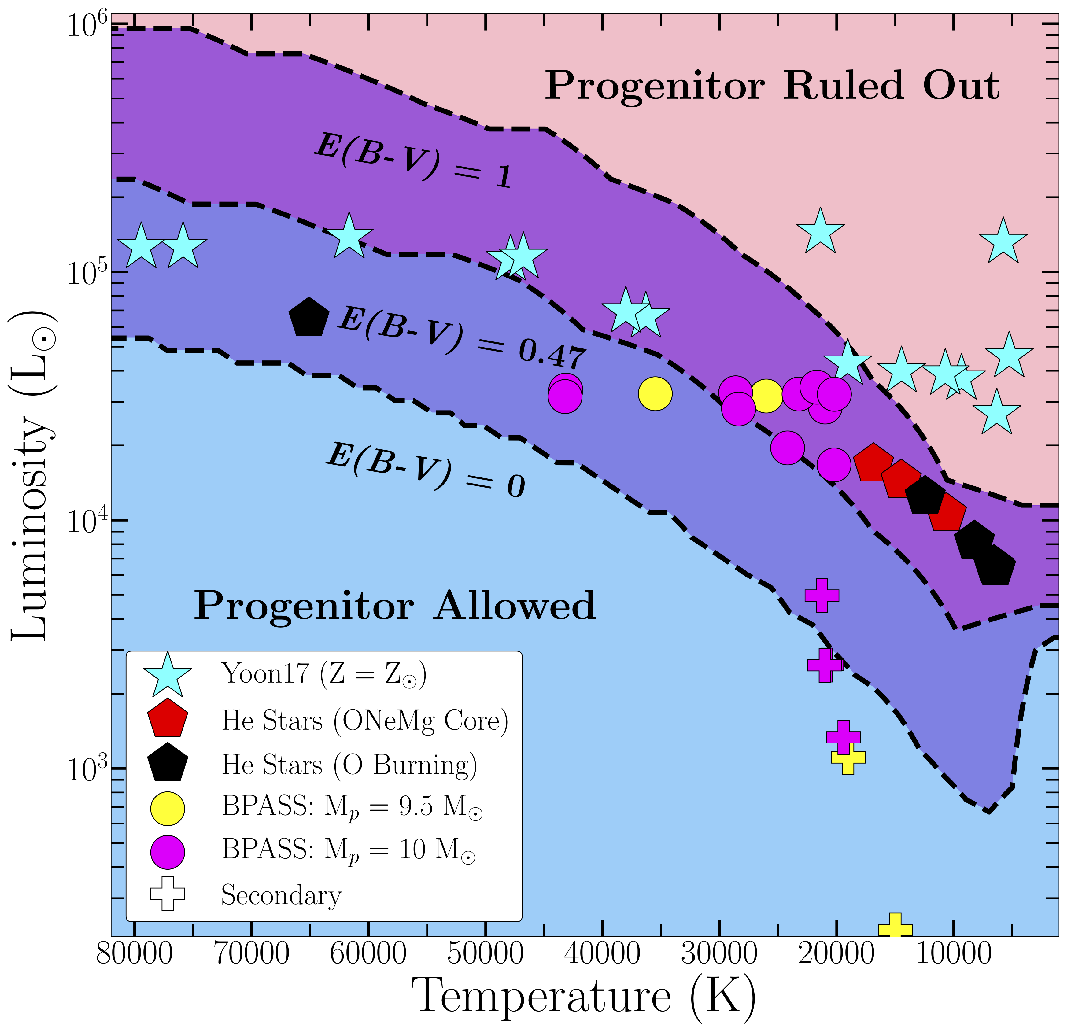
IX Discussion
IX.1 A Physical Progenitor Model
Panchromatic observations have provided an unprecedented picture of this CaST both before and after explosion. In Figure 22, we attempt to combine inferences made from observation and modeling to create a visualization of the explosion and surrounding environment. Our model is a snapshot of the SN at explosion and contains physical scales and parameters such as distance, velocity and composition estimates.
It is most likely the case that the flare is powered by shock interaction or cooling emission in an extended mass of material, regardless of the type of progenitor that exploded. The progenitor could have accrued an extended envelope located at (light grey circle; Fig. 22), while mass-loss in the progenitor’s final months may have placed H- and He-rich material in the circumstellar environment (shown in sea foam green; Fig. 22) with velocities of and at distances cm. The detection of early-time X-ray emission and flash-ionized H and He spectral lines is clear evidence for a SN shock colliding with removed CSM. The observed CSM velocities might be difficult to explain given typical WD escape velocities of needed for mass ejection from a WD surface. However, material might be ejected at low velocities during mass-transfer in WD binaries prior to the merger (see §IX.3).
Based on our modeling of the flare in §VII.3 and §VII.4, we propose a physical scenario that could have produced this first optical light curve peak. In the picture, the flare is powered by two physically distinct emission components: shock interaction with more distant CSM in addition to the cooling of hot, shocked material a smaller radii. Following shock breakout, the inner extended envelope will cool, producing some of the emission on timescales days (blue light curve points; Fig. 22). Once the shock collides with more distant H- and He-rich CSM it will induce “flash-ionized” spectral lines that are powered until 1.5 days via X-ray emission from the shock propagating through the CSM shell. The same low density region of the CSM responsible for X-rays and narrow emission lines can also power the early-time light curve (d). Our analysis has indicated that this shell had a mass of and is located between - cm from the progenitor.
At d, the flare’s power source and the complete explosion picture becomes more ambiguous. By the start of the main peak of the flare (orange light curve points; Fig. 22), the narrow emission lines are no longer detectable and the X-ray emission from the initial shock is rapidly decaying, suggesting that the shock has overtaken the entire CSM shell. Here we propose two plausible expanations for the rapid increase in flux at d. (i) Delayed optical emission from the high density, optically thick regions of the CSM shell begin to cool and radiate in the optical bands following shock interaction. (ii) The shock encounters additional CSM material at cm which induces optical emission from shock interaction.
While this physical progenitor model does account for most of the observables, there are many caveats and unknowns about such a system. First, this model assumes spherically symmetric distributions of mass, both in the inner extended envelope and the outer CSM. Alternatively, this material could have formed a torus where more mass is located in the equatorial regions rather than at the poles. Secondly, neither the shock cooling (§VII.3) nor the shock interaction models (§VII.4) takes into account the chemical composition of the shocked material that then causes the flare. It is likely that the extended masses have significant density gradients, which could lead to variations on how the radiation is able escape the material. Such a scenario would be best tested through numerical modeling (e.g., Piro et al. 2017) in which the density gradients and composition are taken into account, but is ultimately beyond the scope of this paper. Nonetheless, our observations have allowed for the most complete picture of CaST explosion mechanisms and their circumstellar environments. In the following sections we discuss the stellar systems capable of producing the SN 2019ehk observables.
IX.2 Pre-Explosion Constraints on a Massive star Progenitor
Figure 23 shows the constraints on the progenitor system of SN 2019ehk in the H-R diagram, as derived from pre-explosion HST multi-band imaging. In the context of single stars, only compact objects (e.g., WD, NS, BH) and massive stars () are consistent with observations. Specifically, we plot the MESA evolutionary tracks (Choi et al. 2016) of non-rotating single massive stars with the same metallicity as the host galaxy (). We find that only stars with mass 8-10 satisfy the limits for the most extreme choice of intrinsic mag. This is also true for low metallicity stellar tracks with rotation included e.g., dashed goldenrod line of 8 progenitor. However, a more realistic choice of intrinsic mag would effectively rule out the vast majority of parameter space corresponding to various types of single massive stars (). Furthermore, we explore the potential of a single He star progenitor (Table A6) that would be responsible for a core-collapse SN Ib-like explosion. As shown in Figure 24, this model is only consistent with the most highly reddened pre-explosion limits and requires a mechanism to remove its outer H-rich envelope. Overall, we conclude that single massive stars are unlikely progenitors of SN 2019ehk.
We then explore the possibility of a binary progenitor system. To this aim, we employ the large grid of Binary Population and Spectral Synthesis (BPASS) models by Eldridge et al. 2017 to find binary systems that fit the observational parameters of SN 2019ehk. Firstly, we exclude binary models whose final luminosity and temperature do not reside within the “allowed” parameter region of Figure 23 (blue shaded regions). This includes the final luminosity and temperature of both the primary and secondary stars; neither of which should be detected in archival HST imaging. Additionally, we only include systems whose final helium mass is and final hydrogen mass is (e.g., §III.2). To meet the BPASS condition for a resulting SN, we only include systems where the primary’s CO core mass is ¿1.35 and total mass is ¿1.5 . Following these conditions, we look for systems whose ejecta mass is for a weak SN explosion (erg), both of which are inferred from observations (§V.2). When this cut is made on predicted ejecta mass, we recover no consistent binary systems within the SN 2019ehk parameter space. However, because parameters associated with a predicted SN in BPASS are uncertain, we choose to include systems that have a predicted ejecta mass for completeness. We plot the final luminosities and temperatures of 13 potential binary systems in Figure 24 and display significant BPASS parameters of each model in Table A8. Overall, these binary configurations have primary stars with masses of and radii .
We further test the possibility that SN 2019ehk is the result of a more exotic binary system through He-star modeling in MESA. We initialize He-stars with C/O cores and track their luminosity and temperature evolution until the exhaustion of He-burning and the onset of O core burning or the formation of an ONeMg core. We test the following mass-loss scenarios: no mass-loss, standard Wolf-Rayet (WR) winds, artificial envelope removal and binary interaction with NS companion (with varying orbital periods). We present the specifics of each model in Table A6 and plot each final luminosity/temperature as red and black polygons in Figure 24. These are compared to binary models in Yoon et al. 2017 that result in normal SNe Ib/IIb (plotted as cyan stars).
Overall, our presented He-star models are consistent with the pre-explosion parameter space for host extinctions of = 0.5 - 1 mag. We can rule out some of these systems based on the final mass if we assume that the total ejecta mass will be this mass minus 1.4 . The estimated ejecta mass in SN 2019ehk is 0.7 , which is consistent with an artificial envelope removal (models #2, 4) and a He-star + NS binary (models #7,8), both ending in O core burning. However, these models do not naturally reconcile the presence of H-rich CSM in the SN 2019ehk progenitor environment.
We can further constrain the presence of a dusty progenitor for SN 2019ehk by utilizing the Spitzer pre-explosion limits (Table A2). We use the most constraining limit of mag from Channel 2 and assume that the majority of the flux is emitted about an effective wavelength of m. We then apply the spherically symmetric dust shell model shown in Equation 1 of Kilpatrick et al. 2018b. As in their study, we also assume that the dust shell emits isotropically in the optically thin limit (Fox et al. 2010) and have a flux density that goes as , where is the shell mass, is the distance to SN 2019ehk and is the Planck function. Applying this simple approximation, we derive dust shell masses limits of for shell temperatures K, respectively.
Our inferred dust mass is a factor smaller than that derived by Kilpatrick et al. 2018b for LBV outburst Gaia16cfr and an order of magnitude lower than typical dust masses observed around type IIn SNe (Fox et al. 2011). Furthermore, the total dust luminosity of the Gaia16cfr progenitor was L⊙, which is more than an order of magnitude larger than the NIR F160W HST pre-explosion limits (e.g., Fig. 23). Since our derived dust shell mass is similar to Gaia16cfr, a massive star progenitor with a small dust shell would have been detected in pre-explosion images of the SN explosion site. While this analysis is highly simplified, our findings make a dusty progenitor for SN 2019ehk highly unlikely given the observations.
Finally, it should be noted that the luminosity limit derived from Chandra pre-explosion imaging does not constrain the existence of a luminous supersoft X-ray source (SSS) at the location of SN 2019ehk. Such a system has been invoked as a precursor to SNe Ia wherein a nuclear-burning WD accretes mass from a non-degenerate companion. This process in turn produces X-ray luminosities of order erg s-1. However, it has been demonstrated that there are not enough observed SSSs that retain luminous X-ray emission on the same timescale as is needed for quasi-steady burning on the WD surface (Di Stefano 2010). Therefore a single-degenerate scenario, or related event, cannot be constrained with our current Chandra X-ray limits.
From this analysis, we can rule out all single massive stars as progenitors of SN 2019ehk. With regards to binary systems, the pre-explosion parameter space allows for only the lowest mass massive star binaries () or He stars whose envelopes are removed through a mass-loss mechanism. However, while our pre-explosion limits greatly constrain the massive star parameter space, progenitor systems involving a WD cannot be excluded based on detection limits.
IX.3 White Dwarf Explosion Models
Given the pre-explosion limits, every progenitor system involving a WD is permitted in the progenitor parameter space of SN 2019ehk. Nevertheless, we can exclude some of these scenarios based on observed properties of the explosion. As shown in Figure 23, the progenitor of SN Iax, 2012Z is not ruled out and has been proposed to be a He star + WD binary (McCully et al. 2014). However, this progenitor channel cannot account for the H-rich material observed in SN 2019ehk’s circumstellar environment nor the photospheric He in its spectra without significant buildup of unburned He on the WD surface at the time of explosion. Furthermore, explosion models for this configuration generally produce SN Ia, or Iax-like events from failed detonation/deflagration (Jordan et al. 2012; Kromer et al. 2013) that do not match the observed photometric or spectroscopic evolution of CaSTs. The same reasoning rules out a main sequence (MS) companion model typical of SN Ia models. Because common single degenerate progenitor channels appear unlikely for SN 2019ehk, we explore double degenerate explosion scenarios capable of reproducing CaST observables such as those from SN 2019ehk.
Recently, Perets et al. 2019 suggested a double WD (DWD) merger scenario for the origin of SNe Ia, where a CO-WD merges with a hybrid HeCO WD (Zenati et al. 2019b and references therein). In this hybrid + CO DWD (HybCO) model, the disruption of a hybrid WD by a more massive (¿0.75 ) CO WD can give rise to normal SNe Ia (Perets et al. 2019), through a detonation of a He-mixed material on the CO WD surface, followed by a detonation of a CO core due to its compression by the first He-detonation. In cases where the primary WD was of a low mass ( M⊙), only the first He-detonation occurs while the CO core is left intact leaving a remnant WD behind. In such cases, and in particular when the progenitor is a hybrid-WD disrupting a lower-mass CO WD (or another hybrid WD), Zenati et al. 2020 (in prep.) find that the He-detonation gives rise to a faint transient, potentially consistent with CaSTs.
In this specific double-degenerate channel, mass that is lost from the secondary WD prior to its disruption can give rise to CSM, possibly consistent with the observations of SN 2019ehk, as we describe below (a more detailed discussion will be provided in Bobrick et al. 2020, in prep.). This scenario has been explored in the context of SNe Ia wherein the merger is preceded by the ejection of mass as “tidal tails” and placed at distances cm (Raskin & Kasen 2013). Further in, material around the primary WD can “settle down” to form an extended envelope ( cm); this process can occur on timescales of yrs before merger (Shen et al. 2012; Schwab et al. 2016).
Before the actual merger, DWDs spiral-in due to gravitational wave emission. As the binary components gradually come into contact and the donor starts losing mass, the mass transfer rate in the system gradually grows, starting from small values below and continually increasing, which leads to the eventual disruption over several years’ time. Mass-loss during this phase leads to material ejected at typical velocities of likely a few hundreds up to thousand , which expands to characteristic radii of by the time the actual merger happens, while some material could be ejected shortly before the final merger of the WDs. Here we focus on the mass transfer and ejection prior to the merger/disruption of the WDs, which can contribute to the CSM far from the WD and may explain the observations. Levanon & Soker 2017 discussed the possibility of very high velocity CSM from material ejected after the disruption of a WD, and just shortly before the merger; this is however unlikely to explain, or be consistent with, the observations shown here.
We compute the density distribution in the ejecta by solving the equations of secular evolution of the mass transfer rate and binary orbital properties (masses and separation, ) in DWD binaries driven by gravitational wave emission starting from early phases of mass transfer (see e.g., Marsh et al. 2004; Gokhale et al. 2007; Bobrick et al. 2017). We represent the WD donor by one-dimensional, corotating and perfectly-degenerate models following the Helmholtz equation of state Timmes & Swesty 2000 and calculate the mass transfer rate following Kolb & Ritter 1990. The binaries are evolved from the moment mass transfer rate reaches until the mass transfer rate reaches , shortly before the merger. We assume that a fixed fraction of mass is ejected from the systems at some characteristic velocity during the process of mass transfer, both parameters being free parameters of the model.
| Model Name | Abund. | |||
|---|---|---|---|---|
| () | () | (donor) | ||
| Fiducial | CO | |||
| Reduced mass loss | CO | |||
| Fast ejecta | CO | |||
| Heavy accretor | CO | |||
| Hybrid donor | HeCO | |||
| Super-Chandra | CO |
We explored several physically-motivated cases which cover most of the parameter space of possible assumptions in the model, as summarised in Table 3. As the fiducial model, we chose a DWD binary, which represents potential progenitors of CaSTs in the hybCO scenario. In the fiducial model, we assume that % of mass is lost due to direct-impact accretion expected in these binaries and we assigned ejecta velocities of , comparable to the orbital velocity in the binary. In the exploratory models, we considered the cases where only % of mass is lost, where the ejecta is launched at , where the accretor is a CO WD and where the donor is a hybrid HeCO WD , based on the detailed model from Zenati et al. 2019b. Additionally, we simulated a super-Chandrasekhar binary with 0.75+0.95 CO WDs, which is expected to produce brighter SNe Ia instead. As may be seen from Figure 25, the density distributions from the models agree well with the density limits derived from the X-ray detections, flash-ionized spectral lines and radio non-detections. The agreement is also robust to the assumptions in the model, apart from the model with the CO accretor, for which the ejecta density at late times (small radii) disagrees with the X-ray limits. Indeed, this latter case is not expected to give rise to a CaST SN in the HybCO model.
Throughout the evolution, mass transfer gradually peels the donor starting from the outermost layers, and therefore the ejected mass inherits the composition profiles of the donor WD. We use MESA models of WDs stripped during binary evolution and find that CO WDs contain about of H, while hybrid WDs contain less. For example, a HeCO WD model contains only of H and is based on the models from Zenati et al. 2019b. In contrast, models of single WDs predict of surface H (Lawlor & MacDonald 2006) for low-mass WDs ( M⊙) and orders of magnitude lower H abundances on higher mass WDs. Since H is initially in the outermost layer of the donor, it ends up in the outermost parts of the CSM, being replaced-by/mixed-with He at typical separations –, assuming H layers between and . Depending on the mass of the He layer, He is replaced by CO at separations between and , assuming He fraction between and . For hybrid-WDs containing M⊙ of He, no CO is stripped until the final disruption of the hybrid-WD.
The inferred composition of the CSM around SN 2019ehk is broadly consistent with a M⊙ CO or a M⊙ hybrid-WD donor model; both of which formed during binary evolution, and not as isolated single WDs. In particular, these are consistent with the expectations of the HybCO model for CaST SNe progenitors. In the HybCO model interpretation, future observations of CaSTs may potentially be used to put strong constraints on the progenitor systems, and even the surface composition of WDs.
The exact velocity and the geometry of the material lost to the surroundings are the main uncertainties in the pre-merger stripping model. While this material is expected to have velocities comparable to the orbital velocities, the exact detailed hydrodynamical picture of the secular mass-loss in direct-impact DWD binaries is uncertain. In particular, the material may be ejected in an outflow from the disc, a more tightly-collimated jet from near the accretor, or as a more isotropic cloud-like structure powered by the feedback from accretion. When it comes to the fraction of the mass lost from the binary, even within a wide range of assumed efficiencies of mass-loss (range of ejection efficiency), the CSM ejecta profiles agree well with the observations. They explain (i) the cut-off at large separations, due to the time when the secondary WD gradually overfills its Roche lobe and before which no significant stripping initiates; (ii) the overall density profile of the CSM; (iii) the overall composition and the transition between the outer and inner regions due to the compositional structure on the stripped WD surface and (iv) the observed low CSM velocities derived from early-time H and He II lines. It should also be noted that similar observables could be obtained from the disruption of HybCO (hybrid He/C/O) WD by a NS (e.g., see Fernández et al. 2019) although the rates associated with such binary systems are not consistent with CaSTs.
IX.4 Tidal Disruption by an Intermediate-Mass Black Hole
A proposed model for CaSTs is the tidal disruption of a low mass WD by an intermediate mass black hole (IMBH) (Rosswog et al. 2008; Metzger 2012; MacLeod et al. 2014; Sell et al. 2015; Tanikawa et al. 2017). One prominent signature of this accretion process would be the presence of X-ray emission above the Eddington luminosity. Since we observed luminous X-ray emission from the CaSTs SN 2019ehk for the first time, we briefly discuss this scenario here. Sell et al. 2015 first explore this scenario for the CaST 2012hn to constrain the potential masses of the IMBH and of the disrupted WD via X-ray upper limits at 533 days after explosion. Milisavljevic et al. 2017 employ a similar method for iPTF15eqv, for which these authors infer an IMBH mass on an accretion timescale of ¡164 days. We apply the same method to SN 2019ehk here.
The X-ray luminosity of SN 2019ehk at days since explosion (Figure 7) is consistent with the Eddington luminosity of a BH, for which the timescale of fallback accretion is (e.g. Milisavljevic et al. 2017):
| (19) |
which indicates that for fiducial values of and , such a transient would have an accretion luminosity above the Eddington limit for 1 yr. This timescale is not consistent with observations of SN 2019ehk as its X-ray emission fades quickly on timescales of days as after the first detection. The IMBH scenario can be further constrained by using the deepest X-ray luminosity limit of erg s-1 obtained with Chandra at days since explosion. Using d (the phase of observation), we calculate a limit on the BH mass of , assuming fiducial WD parameters. From the X-ray luminosity limit, and assuming an accretion efficiency of , we calculate a BH mass limit of . Furthermore, as discussed in §VIII, we find no evidence for an off-axis jet in our modeling of the radio emission, which is assumed to be associated with an accretion event such as the tidal disruption of a WD by an IMBH. Lastly, a IMBH progenitor is expected to be associated with a cluster, yet we find no sources near the SN location in the pre-explosion images. Based on these inferences, we conclude that the tidal disruption of a WD by an IMBH is an extremely unlikely physical scenario for SN 2019ehk.
IX.5 SN 2019ehk in the “Calcium-strong” Class
SN 2019ehk is currently the CaST with the most extended and detailed observational data set across the electromagnetic spectrum. A key question is how representative SN 2019ehk is of the entire “Calcium-strong” class of transients? As discussed in §V.1, the optical light curve ( mag, m mag) and color evolution of SN 2019ehk are consistent with the class of CaSTs (e.g., Figures 8 & 10). However, the main photometric difference is its prominent double (triple?) peaked light curve with the initial “flare” only matching one other object in the class, iPTF16hgs (De et al. 2019). iPTF16hgs was not discovered as early but does show consistency spectroscopically (Figure 14(a)) to SN 2019ehk. Both objects were found in star forming host galaxy environments, in contrast with the majority of the sample (e.g. Shen et al. 2019). Furthermore, De et al. 2018 also find that shock breakout emission can reproduce the increase in flux prior to the Ni-powered light peak. These combined similarities suggest a shared progenitor scenario amongst these two objects (and potentially other CaSTs).
Spectroscopically, SN 2019ehk shows near remarkable consistency with CaSTs SNe 2005E and 2007ke (Figure 14b). This level of similarity is intriguing given that the large-scale environments of these two CaSTs relative to SN 2019ehk are quite different (SNe 2005E and 2007ke are located on the outskirts of early-type galaxies while SN 2019ehk is embedded in a late-type spiral galaxy). SN 2005E was modeled via a helium shell detonation of a sub-Chandra WD (Perets et al. 2010b; Waldman et al. 2011), and SN 2007ke is thought to arise from a compact object progenitor given the lack of star formation at its explosion site (Lunnan et al. 2017). Generally, SN 2019ehk shares clear spectroscopic similarities with the rest of the class: Type I spectrum, visible He I, weak Fe-group element and O I transitions, and dominant Ca II emission at late-times. SN 2019ehk has the largest [Ca II]/[O I] ratio yet observed amongst CaSTs (and known transients as a whole) and has the earliest visible detection of [Ca II] (-5 days). Out to nebular times, SN 2019ehk shows persistent [Ca II] emission that is similar to other CaSTs. Therefore, SN 2019ehk’s [Ca II]/[O I] ratio is consistent with the overall classification of CaSTs and it is the “richest” known object in Ca emission.
SN 2019ehk is located in a star-forming region of a barred spiral host-galaxy. SN 2019ehk thus adds to the increasing evidence for a wide distribution of both early and late type host galaxies for CaSTs. The SN is also embedded in its host galaxy (offset 2 kpc), which suggests that CaST class cannot be completely defined by large galactic offsets. Overall, a large fraction of the current CaSTs sample are located at large offsets from early-type galaxies and/or with limited to no visible star formation (Perets et al. 2010a; Perets et al. 2011; Kasliwal et al. 2012; Lyman et al. 2013; Lyman et al. 2014; Lunnan et al. 2017; De et al. 2020). However, multiple confirmed CaSTs and candidate objects have deviated from this trend. iPTF15eqv, iPTF16hgs and SN 2016hnk are all located in spiral host-galaxies and analysis of the explosion sites indicate the presence of star formation (Milisavljevic et al. 2017; De et al. 2018; Galbany et al. 2019; Jacobson-Galan et al. 2019). Similarly, CaSTs PTF09dav, SN 2001co, SN 2003H, SN 2003dr and 2003dg appear to have exploded in or offset from disk-galaxies (Sullivan et al. 2011; Kasliwal et al. 2012; Perets 2014; Foley 2015).
The older stellar populations where a large fraction of CaSTs are found makes it difficult to reconcile a massive star progenitor for the entire class. In the context of WD progenitors, the increased discovery of CaSTs in late-type galaxies with a young stellar population component is still compatible with an older progenitor given the frequency of WDs in a variety of host environments. A larger sample of stellar ages near CaST explosion sites will confirm whether a broad(er) delay time distribution is needed to explain the presence of some CaSTs in younger stellar populations. Nevertheless, the existence of star-forming host galaxies does potentially still allow for a massive stellar progenitor channel (and hence a core-collapse origin) as an explanation for some CaSTs, as suggested by Milisavljevic et al. 2017. SN 2019ehk has greatly constrained the massive star progenitor parameter space by illustrating that only the lowest mass stars (8-10 ) in binary systems are permitted progenitors of a CaST. Increasing the sample size of CaSTs with detailed observational coverage across the spectrum will help to reveal whether this class truly has multiple associated progenitor scenarios.
Finally, the detection of luminous X-ray emission in SN 2019ehk represents a newly discovered observational signature of CaSTs. Based on the observational coverage at X-ray wavelengths, it has become apparent that CaSTs may only exhibit X-ray emission at very early-times. No other CaSTs has X-ray observations before +25d after explosion yet we now know that X-ray emission in SN 2019ehk only lasted until +4 days. This indicates two possibilities: the explosion and environment of SN 2019ehk are unique or CaSTs do show X-ray emission directly after explosion that has been missed observationally until now. If the latter is true, then extremely early observations of CaSTs is imperative to understand the progenitor environments of these objects.
X Summary and Conclusions
In this paper we have presented pre- and post-explosion (0.4-292 days) panchromatic observations of the nearby CaST SN 2019ehk located in a region of high star formation near the core of the SAB(rs)c galaxy M100 at Mpc. Our observations cover the electromagnetic spectrum from the X-rays to the radio band, before and after the explosion. Below we summarize the primary observational findings that make SN 2019ehk the CaST with the richest data set to date:
- •
SN 2019ehk was detected 0.44 days after explosion and its UV/optical/NIR photometric evolution shows a double-peaked light curve in all multi-color bands, similar to CaST iPTF16hgs (De et al. 2018). However, different from iPTF16hgs, these very early observations of SN 2019ehk were also able to capture the rapid rise to the first light curve peak. With respect to its second broader light curve peak, SN 2019ehk has a rise-time days, a peak -band magnitude mag and Phillips 1993 decline parameter of m15(B) = 1.71 mag.
- •
Within 24 hrs of discovery, three optical spectra were acquired starting at days since explosion, and revealed the rapid disappearance of “flash-ionized” H Balmer series and He II emission lines with velocities of and , respectively. These spectral features were detected at the time of the first light curve peak, and provide first evidence for H+He-rich CSM in the immediate vicinity of a CaST.
- •
SN 2019ehk showed luminous, rapidly-decaying X-ray emission ( erg s-1 with ). The luminous X-ray emission detected with Swift-XRT at +3 and +4d after explosion constitutes a newly discovered observational signature of CaSTs and results from the exploration of a pristine portion of the X-ray parameter space within this class. The X-ray emission is temporally coincident with the first optical light curve peak (“the flare”). At later times (+292d) Chandra observations provided the deepest constraints on a CaST to date ( erg s-1).
- •
Our deep radio monitoring with the VLA provided the tightest constraints on the radio luminosity from a CaST at phases ¿30 days after explosion .
- •
SN 2019ehk has the latest spectroscopic follow-up of any CaST at +257d after explosion. The spectrum revealed the largest [Ca II]/[O I] line flux ratio yet reported ().
- •
The explosion site of SN 2019ehk has extremely deep pre-explosion imaging with Chandra, Spitzer and HST. No source is detected in any archival image with an astrometric uncertainty of and .
By modeling these observations we place tight constraints on the SN progenitor, its environment and the explosion mechanism:
- •
Bolometric light curve models show that the explosion synthesized of , produced of ejecta and had a kinetic energy of erg.
- •
The H+He-rich material is part of the CSM and preceded the SN explosion. “Flash-ionized” emission lines indicate the presence of pre-shock CSM gas with mass and composition in the range by number. The total CSM mass as inferred from X-ray observations is , comprised of and of H- and He-rich material, respectively. Both observations combined revealed a CSM density of g cm-3 at cm.
- •
For realistic microphysical parameters ( and ), radio non-detections suggest a mass-loss rate of for a wind velocity at distances cm from the explosion site.
- •
We model the early-time optical emission with two models: (i) shock interaction with CSM and (ii) shock cooling following breakout into extended material. Given an observed SN ejecta mass , the former yields a CSM mass of and radius of cm. This model can adequately power the persistent SN optical emission at d and is consistent with the duration of visible H+He emission lines. The latter model provides a potential physical mechanism for the increased optical emission at d and indicates extended material of mass and radius . These values are broadly consistent with our inferences from the H+He spectral lines and the modeling of the X-ray emission, suggesting that the presence of an extended distribution of (H+He rich) material with which the SN shock interacted can reasonably account for three key observational findings in SN 2019ehk (e.g., the X-ray emission, the optical flare and the transient H+He lines).
Pre-explosion imaging at the location of SN 2019ehk rules out a vast portion of the parameter space associated with both massive stars and WD explosions. Specifically, we find that pre-explosion limits rule out all single massive stars with mass as the progenitor of CaST SN 2019ehk for a host reddening of . We explore the available binary system parameter space and find that our limits only allow for systems with a primary star or a low-mass He star whose envelope was removed through mass-loss and/or binary interaction. Furthermore, the observed explosion properties make it unlikely that SN 2019ehk was produced by the explosion of a C/O WD with a He or main sequence star companion. However, we find that a model for the disruption of a low-mass C/O WD or a hybrid HeCO WD () by another, likely low-mass hybrid WD is consistent with the CSM densities, abundances and dynamics inferred for SN 2019ehk, and would possibly be able to account for the increasingly large fraction of CaSTs embedded in young stellar populations by allowing for a broader time delay distribution. Complete multi-wavelength observations of future CaSTs will be instrumental in differentiating between these two possible progenitor scenarios.
XI Acknowledgements
We thank David Matthews, Enrico Ramirez-Ruiz, Brian Metzger and Nathan Smith for stimulating conversations and constructive comments in regards to this work.
W.J-G is supported by the National Science Foundation Graduate Research Fellowship Program under Grant No. DGE-1842165 and the Data Science Initiative Fellowship from Northwestern University. R.M. is grateful to KITP for hospitality during the completion of this paper. This research was supported in part by the National Science Foundation under Grant No. NSF PHY-1748958. R.M. acknowledges support by the National Science Foundation under Award No. AST-1909796. Raffaella Margutti is a CIFAR Azrieli Global Scholar in the Gravity & the Extreme Universe Program, 2019. The Margutti’s team at Northwestern is partially funded by the Heising-Simons Foundation under grant # 2018-0911 (PI: Margutti).
The National Radio Astronomy Observatory is a facility of the National Science Foundation operated under cooperative agreement by Associated Universities, Inc. GMRT is run by the National Centre for Radio Astrophysics of the Tata Institute of Fundamental Research.
The scientific results reported in this article are based in part on observations made by the Chandra X-ray Observatory. This research has made use of software provided by the Chandra X-ray Center (CXC) in the application packages CIAO. Partial support for this work was provided by the National Aeronautics and Space Administration through Chandra Award Number DD0-21114X issued by the Chandra X-ray Center, which is operated by the Smithsonian Astrophysical Observatory for and on behalf of the National Aeronautics Space Administration under contract NAS8-03060.
W. M. Keck Observatory [and/or MMT Observatory] access was supported by Northwestern University and the Center for Interdisciplinary Exploration and Research in Astrophysics (CIERA).
The UCSC transient team is supported in part by NSF grant AST-1518052, NASA/Swift grant 80NSSC19K1386, the Gordon & Betty Moore Foundation, the Heising-Simons Foundation, and by a fellowship from the David and Lucile Packard Foundation to R.J.F. Research at Lick Observatory is partially supported by a generous gift from Google.
A.H. is partially supported by the Future Investigators in NASA Earth and Space Science and Technology (FINESST) Award No. 80NSSC19K1422. HBP acknowledges support from the Kingsely distinguished-visitor program at Caltech, and the KITP visitor program. KJS is supported by NASA through the Astrophysics Theory Program (NNX17AG28G). PJB is supported by a NASA Swift Guest Investigator grant 80NSSC19K0316. TMB was funded by the CONICYT PFCHA / DOCTORADOBECAS CHILE/2017-72180113. SCY is supported by the National Research Foundation of Korea (NRF) grant (NRF-2019R1A2C2010885). MG is supported by the Polish NCN MAESTRO grant 2014/14/A/ST9/00121. DAH, JB, DH, and CP are supported by NSF AST-1911225 and NASA grant 80NSSC19K1639. JD and EB are supported in part by NASA Grant 80NSSC20K0456. SJS acknowledges funding from STFC Grant ST/P000312/1. M.R.S. is supported by the National Science Foundation Graduate Research Fellowship Program under Grant No. 1842400.
Research by DJS is supported by NSF grants AST-1821967, 1821987, 1813708, 1813466, and 1908972. This research is based on observations made with the NASA/ESA Hubble Space Telescope obtained from the Space Telescope Science Institute, which is operated by the Association of Universities for Research in Astronomy, Inc., under NASA contract NAS 5-26555. These observations are associated with program 15645.
X. Wang is supported by the National Natural Science Foundation of China (NSFC grants 11325313, 11633002, and 11761141001), and the National Program on Key Research and Development Project (grant no. 2016YFA0400803). We acknowledge the support of the staff of the Xinglong 2.16-m telescope. This work was partially supported by the Open Project Program of the Key Laboratory of Optical Astronomy, National Astronomical Observatories, Chinese Academy of Sciences.” Funding for the LJT has been provided by Chinese Academy of Sciences and the People’s Government of Yunnan Province. The LJT is jointly operated and administrated by Yunnan Observatories and Center for Astronomical Mega-Science, CAS.
Based on observations obtained at the Southern Astrophysical Research (SOAR) telescope, which is a joint project of the Ministério da Ciência, Tecnologia, Inovações e Comunicações (MCTIC) do Brasil, the U.S. National Optical Astronomy Observatory (NOAO), the University of North Carolina at Chapel Hill (UNC), and Michigan State University (MSU).
Observations reported here were obtained at the MMT Observatory, a joint facility of the University of Arizona and the Smithsonian Institution.
Some of the data presented herein were obtained at the W. M. Keck Observatory, which is operated as a scientific partnership among the California Institute of Technology, the University of California and the National Aeronautics and Space Administration. The Observatory was made possible by the generous financial support of the W. M. Keck Foundation. The authors wish to recognize and acknowledge the very significant cultural role and reverence that the summit of Maunakea has always had within the indigenous Hawaiian community. We are most fortunate to have the opportunity to conduct observations from this mountain. We wish to recognize the destructive history of colonialism endured by native Hawaiians as we strive to hear the voice of those whose sacred land we continue to utilize for scientific gain.
This work includes data obtained with the Swope Telescope at Las Campanas Observatory, Chile, as part of the Swope Time Domain Key Project (PI: Piro, Co-Is: Drout, Phillips, Holoien, French, Cowperthwaite, Burns, Madore, Foley, Kilpatrick, Rojas-Bravo, Dimitriadis, Hsiao). We wish to thank Swope Telescope observers Jorge Anais Vilchez, Abdo Campillay, Nahir Munoz Elgueta and Natalie Ulloa for collecting data presented in this paper.
This research has made use of the XRT Data Analysis Software (XRTDAS) developed under the responsibility of the ASI Science Data Center (ASDC), Italy. The SN group at Konkoly Observatory is supported by the project “Transient Astrophysical Objects” GINOP 2.3.2-15-2016-00033 of the National Research, Development and Innovation Office (NKFIH), Hungary, funded by the European Union. Based on observations collected at the European Southern Observatory under ESO programme 1103.D-0328.
This work has made use of data from the Asteroid Terrestrial-impact Last Alert System (ATLAS) project. ATLAS is primarily funded to search for near earth asteroids through NASA grants NN12AR55G, 80NSSC18K0284, and 80NSSC18K1575; byproducts of the NEO search include images and catalogs from the survey area. The ATLAS science products have been made possible through the contributions of the University of Hawaii Institute for Astronomy, the Queen’s University Belfast, and the Space Telescope Science Institute.
References
- Albareti et al. (2017) Albareti, F. D., Allende Prieto, C., Almeida, A., et al. 2017, ApJS, 233, 25
- Almgren et al. (2010) Almgren, A. S., Beckner, V. E., Bell, J. B., et al. 2010, ApJ, 715, 1221
- Arcavi et al. (2011) Arcavi, I., Gal-Yam, A., Yaron, O., et al. 2011, ApJ, 742, L18
- Arcavi et al. (2017) Arcavi, I., Hosseinzadeh, G., Brown, P. J., et al. 2017, ApJ, 837, L2
- Arnett (1982) Arnett, W. D. 1982, ApJ, 253, 785
- Becker (2015) Becker, A. 2015, HOTPANTS: High Order Transform of PSF ANd Template Subtraction, Astrophysics Source Code Library, , , ascl:1504.004
- Bellm et al. (2019) Bellm, E. C., Kulkarni, S. R., Graham, M. J., et al. 2019, PASP, 131, 018002
- Benjamin et al. (1999) Benjamin, R. A., Skillman, E. D., & Smits, D. P. 1999, ApJ, 514, 307
- Bertin & Arnouts (1996) Bertin, E., & Arnouts, S. 1996, A&AS, 117, 393
- Blondin & Tonry (2007) Blondin, S., & Tonry, J. L. 2007, ApJ, 666, 1024
- Bobrick et al. (2017) Bobrick, A., Davies, M. B., & Church, R. P. 2017, MNRAS, 467, 3556
- Brown et al. (2014) Brown, P. J., Breeveld, A. A., Holland, S., Kuin, P., & Pritchard, T. 2014, Ap&SS, 354, 89
- Burrows et al. (2005) Burrows, D. N., Hill, J. E., Nousek, J. A., et al. 2005, Space Sci. Rev., 120, 165
- Buzzoni et al. (1984) Buzzoni, B., Delabre, B., Dekker, H., et al. 1984, The Messenger, 38, 9
- Cao et al. (2013) Cao, Y., Kasliwal, M. M., Arcavi, I., et al. 2013, ApJ, 775, L7
- Cappellaro et al. (1997) Cappellaro, E., Mazzali, P. A., Benetti, S., et al. 1997, A&A, 328, 203
- Chatzopoulos et al. (2016) Chatzopoulos, E., Wheeler, J. C., Vinko, J., et al. 2016, ApJ, 828, 94
- Chevalier (1998) Chevalier, R. A. 1998, ApJ, 499, 810
- Choi et al. (2016) Choi, J., Dotter, A., Conroy, C., et al. 2016, ApJ, 823, 102
- Chomiuk et al. (2012) Chomiuk, L., Soderberg, A. M., Moe, M., et al. 2012, ApJ, 750, 164
- Chomiuk et al. (2016) Chomiuk, L., Soderberg, A. M., Chevalier, R. A., et al. 2016, ApJ, 821, 119
- Cid Fernandes et al. (2005) Cid Fernandes, R., Mateus, A., Sodré, L., Stasińska, G., & Gomes, J. M. 2005, MNRAS, 358, 363
- Clemens et al. (2004) Clemens, J. C., Crain, J. A., & Anderson, R. 2004, Society of Photo-Optical Instrumentation Engineers (SPIE) Conference Series, Vol. 5492, The Goodman spectrograph, ed. A. F. M. Moorwood & M. Iye, 331–340
- Crowther (2007) Crowther, P. A. 2007, ARA&A, 45, 177
- Cushing et al. (2004) Cushing, M. C., Vacca, W. D., & Rayner, J. T. 2004, PASP, 116, 362
- De et al. (2018) De, K., Kasliwal, M. M., Cantwell, T., et al. 2018, ApJ, 866, 72
- De et al. (2019) De, K., Kasliwal, M. M., Polin, A., et al. 2019, ApJ, 873, L18
- De et al. (2020) De, K., Kasliwal, M. M., Tzanidakis, A., et al. 2020, arXiv e-prints, arXiv:2004.09029
- Di Stefano (2010) Di Stefano, R. 2010, ApJ, 712, 728
- Dimitriadis et al. (2019) Dimitriadis, G., Siebert, M. R., Kilpatrick, C. D., et al. 2019, The Astronomer’s Telegram, 12707, 1
- Dopita et al. (2016) Dopita, M. A., Kewley, L. J., Sutherland, R. S., & Nicholls, D. C. 2016, Ap&SS, 361, 61
- Drory (2003) Drory, N. 2003, A&A, 397, 371
- Drout et al. (2016) Drout, M. R., Milisavljevic, D., Parrent, J., et al. 2016, ApJ, 821, 57
- Eldridge et al. (2017) Eldridge, J. J., Stanway, E. R., Xiao, L., et al. 2017, PASA, 34, e058
- Fabricant et al. (2019) Fabricant, D., Fata, R., Epps, H., et al. 2019, PASP, 131, 075004
- Fan et al. (2015) Fan, Y.-F., Bai, J.-M., Zhang, J.-J., et al. 2015, Research in Astronomy and Astrophysics, 15, 918
- Fernández et al. (2019) Fernández, R., Margalit, B., & Metzger, B. D. 2019, MNRAS, 488, 259
- Filippenko et al. (2003) Filippenko, A. V., Chornock, R., Swift, B., et al. 2003, IAU Circ., 8159, 2
- Fink et al. (2010) Fink, M., Röpke, F. K., Hillebrandt, W., et al. 2010, A&A, 514, A53
- Fitzpatrick (1999) Fitzpatrick, E. L. 1999, PASP, 111, 63
- Flewelling et al. (2016a) Flewelling, H. A., Magnier, E. A., Chambers, K. C., et al. 2016a, arXiv e-prints, arXiv:1612.05243
- Flewelling et al. (2016b) —. 2016b, arXiv e-prints, arXiv:1612.05243
- Folatelli et al. (2010) Folatelli, G., Phillips, M. M., Burns, C. R., et al. 2010, AJ, 139, 120
- Foley (2015) Foley, R. J. 2015, MNRAS, 452, 2463
- Foley et al. (2016) Foley, R. J., Jha, S. W., Pan, Y.-C., et al. 2016, MNRAS, 461, 433
- Foley et al. (2003) Foley, R. J., Papenkova, M. S., Swift, B. J., et al. 2003, PASP, 115, 1220
- Foley et al. (2009) Foley, R. J., Chornock, R., Filippenko, A. V., et al. 2009, AJ, 138, 376
- Foreman-Mackey et al. (2013) Foreman-Mackey, D., Hogg, D. W., Lang, D., & Goodman, J. 2013, PASP, 125, 306
- Fox et al. (2010) Fox, O. D., Chevalier, R. A., Dwek, E., et al. 2010, ApJ, 725, 1768
- Fox et al. (2011) Fox, O. D., Chevalier, R. A., Skrutskie, M. F., et al. 2011, ApJ, 741, 7
- Freedman et al. (2001) Freedman, W. L., Madore, B. F., Gibson, B. K., et al. 2001, ApJ, 553, 47
- Fremling et al. (2016) Fremling, C., Sollerman, J., Taddia, F., et al. 2016, A&A, 593, A68
- Frohmaier et al. (2018) Frohmaier, C., Sullivan, M., Maguire, K., & Nugent, P. 2018, ApJ, 858, 50
- Gal-Yam et al. (2014) Gal-Yam, A., Arcavi, I., Ofek, E. O., et al. 2014, Nature, 509, 471
- Galbany et al. (2016) Galbany, L., Anderson, J. P., Rosales-Ortega, F. F., et al. 2016, MNRAS, 455, 4087
- Galbany et al. (2018) Galbany, L., Anderson, J. P., Sánchez, S. F., et al. 2018, ApJ, 855, 107
- Galbany et al. (2019) Galbany, L., Ashall, C., Hoeflich, P., et al. 2019, arXiv e-prints, arXiv:1904.10034
- Gehrels et al. (2004) Gehrels, N., Chincarini, G., Giommi, P., et al. 2004, ApJ, 611, 1005
- Gokhale et al. (2007) Gokhale, V., Peng, X. M., & Frank, J. 2007, ApJ, 655, 1010
- Gonzaga (2012) Gonzaga, S. 2012, The DrizzlePac Handbook
- Graham et al. (2019) Graham, M. J., Kulkarni, S. R., Bellm, E. C., et al. 2019, PASP, 131, 078001
- Guevel & Hosseinzadeh (2017) Guevel, D., & Hosseinzadeh, G. 2017, dguevel/PyZOGY: Initial release, vv0.0.1, Zenodo, doi:10.5281/zenodo.1043973. https://doi.org/10.5281/zenodo.1043973
- Guillochon et al. (2018) Guillochon, J., Nicholl, M., Villar, V. A., et al. 2018, ApJS, 236, 6
- Ho et al. (2019) Ho, A. Y. Q., Goldstein, D. A., Schulze, S., et al. 2019, ApJ, 887, 169
- Holcomb et al. (2013) Holcomb, C., Guillochon, J., De Colle, F., & Ramirez-Ruiz, E. 2013, ApJ, 771, 14
- Horne (1986) Horne, K. 1986, PASP, 98, 609
- Howell et al. (2005) Howell, D. A., Sullivan, M., Perrett, K., et al. 2005, ApJ, 634, 1190
- Hummer & Storey (1987) Hummer, D. G., & Storey, P. J. 1987, MNRAS, 224, 801
- Jacobson-Galan et al. (2019) Jacobson-Galan, W. V., Polin, A., Foley, R. J., et al. 2019, arXiv e-prints, arXiv:1910.05436
- Jordan et al. (2012) Jordan, George C., I., Perets, H. B., Fisher, R. T., & van Rossum, D. R. 2012, ApJ, 761, L23
- Julienne et al. (1974) Julienne, P. S., Davis, J., & Oran, E. 1974, J. Geophys. Res., 79, 2540
- Kalberla et al. (2005) Kalberla, P. M. W., Burton, W. B., Hartmann, D., et al. 2005, A&A, 440, 775
- Kasen et al. (2006) Kasen, D., Thomas, R. C., & Nugent, P. 2006, ApJ, 651, 366
- Kasliwal et al. (2013) Kasliwal, M., Cao, Y., Surace, J., et al. 2013, SPIRITS: SPitzer InfraRed Intensive Transients Survey, Spitzer Proposal, ,
- Kasliwal et al. (2014) Kasliwal, M., Cao, Y., Masci, F., et al. 2014, SPIRITS: SPitzer InfraRed Intensive Transients Survey, Spitzer Proposal, ,
- Kasliwal et al. (2016) Kasliwal, M., Lau, R., Cao, Y., et al. 2016, SPIRITS: SPitzer InfraRed Intensive Transients Survey, Spitzer Proposal, ,
- Kasliwal et al. (2018) Kasliwal, M., Jencson, J., Lau, R., et al. 2018, SPIRITS: SPitzer InfraRed Intensive Transients Survey, Spitzer Proposal, ,
- Kasliwal et al. (2012) Kasliwal, M. M., Kulkarni, S. R., Gal-Yam, A., et al. 2012, ApJ, 755, 161
- Kennicutt (1998) Kennicutt, Robert C., J. 1998, ARA&A, 36, 189
- Kewley & Ellison (2008) Kewley, L. J., & Ellison, S. L. 2008, ApJ, 681, 1183
- Kilpatrick et al. (2018a) Kilpatrick, C. D., Takaro, T., Foley, R. J., et al. 2018a, MNRAS, 480, 2072
- Kilpatrick et al. (2018b) Kilpatrick, C. D., Foley, R. J., Drout, M. R., et al. 2018b, MNRAS, 473, 4805
- Kochanek (2019) Kochanek, C. S. 2019, MNRAS, 483, 3762
- Kolb & Ritter (1990) Kolb, U., & Ritter, H. 1990, A&A, 236, 385
- Kromer et al. (2013) Kromer, M., Fink, M., Stanishev, V., et al. 2013, MNRAS, 429, 2287
- Kuncarayakti et al. (2018) Kuncarayakti, H., Anderson, J. P., Galbany, L., et al. 2018, A&A, 613, A35
- Lang et al. (2010) Lang, D., Hogg, D. W., Mierle, K., Blanton, M., & Roweis, S. 2010, AJ, 139, 1782
- Lawlor & MacDonald (2006) Lawlor, T. M., & MacDonald, J. 2006, MNRAS, 371, 263
- Levanon & Soker (2017) Levanon, N., & Soker, N. 2017, MNRAS, 470, 2510
- Liu et al. (2018) Liu, L.-D., Zhang, B., Wang, L.-J., & Dai, Z.-G. 2018, ApJ, 868, L24
- Lundqvist & Fransson (1996) Lundqvist, P., & Fransson, C. 1996, ApJ, 464, 924
- Lunnan et al. (2017) Lunnan, R., Kasliwal, M. M., Cao, Y., et al. 2017, ApJ, 836, 60
- Lyman et al. (2013) Lyman, J. D., James, P. A., Perets, H. B., et al. 2013, MNRAS, 434, 527
- Lyman et al. (2014) Lyman, J. D., Levan, A. J., Church, R. P., Davies, M. B., & Tanvir, N. R. 2014, MNRAS, 444, 2157
- MacLeod et al. (2014) MacLeod, M., Goldstein, J., Ramirez-Ruiz, E., Guillochon, J., & Samsing, J. 2014, ApJ, 794, 9
- Malesani et al. (2009) Malesani, D., Fynbo, J. P. U., Hjorth, J., et al. 2009, ApJ, 692, L84
- Margalit & Metzger (2016) Margalit, B., & Metzger, B. D. 2016, MNRAS, 461, 1154
- Margutti et al. (2013) Margutti, R., Zaninoni, E., Bernardini, M. G., et al. 2013, MNRAS, 428, 729
- Marsh et al. (2004) Marsh, T. R., Nelemans, G., & Steeghs, D. 2004, MNRAS, 350, 113
- Massey et al. (2015) Massey, P., Neugent, K. F., & Morrell, N. 2015, ApJ, 807, 81
- Matzner & McKee (1999) Matzner, C. D., & McKee, C. F. 1999, ApJ, 510, 379
- Maund et al. (2011) Maund, J. R., Fraser, M., Ergon, M., et al. 2011, ApJ, 739, L37
- McCully et al. (2014) McCully, C., Jha, S. W., Foley, R. J., et al. 2014, Nature, 512, 54
- McMullin et al. (2007) McMullin, J. P., Waters, B., Schiebel, D., Young, W., & Golap, K. 2007, in Astronomical Society of the Pacific Conference Series, Vol. 376, Astronomical Data Analysis Software and Systems XVI, ed. R. A. Shaw, F. Hill, & D. J. Bell, 127
- Metzger (2012) Metzger, B. D. 2012, MNRAS, 419, 827
- Milisavljevic et al. (2015) Milisavljevic, D., Margutti, R., Kamble, A., et al. 2015, ApJ, 815, 120
- Milisavljevic et al. (2017) Milisavljevic, D., Patnaude, D. J., Raymond, J. C., et al. 2017, ApJ, 846, 50
- Modjaz et al. (2009) Modjaz, M., Li, W., Butler, N., et al. 2009, ApJ, 702, 226
- Nakar & Piro (2014) Nakar, E., & Piro, A. L. 2014, ApJ, 788, 193
- Neugent et al. (2012) Neugent, K. F., Massey, P., Skiff, B., & Meynet, G. 2012, ApJ, 749, 177
- Nicholl et al. (2019) Nicholl, M., Short, P., Angus, C. R., et al. 2019, The Astronomer’s Telegram, 12697, 1
- Nomoto (1982) Nomoto, K. 1982, ApJ, 257, 780
- Oke et al. (1995) Oke, J. B., Cohen, J. G., Carr, M., et al. 1995, PASP, 107, 375
- Osterbrock & Ferland (2006) Osterbrock, D. E., & Ferland, G. J. 2006, Astrophysics of gaseous nebulae and active galactic nuclei
- Perets (2014) Perets, H. B. 2014, arXiv e-prints, arXiv:1407.2254
- Perets et al. (2011) Perets, H. B., Badenes, C., Arcavi, I., Simon, J. D., & Gal-yam, A. 2011, ApJ, 730, 89
- Perets et al. (2019) Perets, H. B., Zenati, Y., Toonen, S., & Bobrick, A. 2019, arXiv e-prints, arXiv:1910.07532
- Perets et al. (2010a) Perets, H. B., Gal-Yam, A., Mazzali, P. A., et al. 2010a, Nature, 465, 322
- Perets et al. (2010b) —. 2010b, Nature, 465, 322
- Pettini & Pagel (2004) Pettini, M., & Pagel, B. E. J. 2004, MNRAS, 348, L59
- Phillips (1993) Phillips, M. M. 1993, ApJ, 413, L105
- Piro (2015) Piro, A. L. 2015, ApJ, 808, L51
- Piro et al. (2017) Piro, A. L., Muhleisen, M., Arcavi, I., et al. 2017, ApJ, 846, 94
- Pohlen et al. (2010) Pohlen, M., Cortese, L., Smith, M. W. L., et al. 2010, A&A, 518, L72
- Polin et al. (2019a) Polin, A., Nugent, P., & Kasen, D. 2019a, arXiv e-prints, arXiv:1910.12434
- Polin et al. (2019b) —. 2019b, ApJ, 873, 84
- Poznanski et al. (2012) Poznanski, D., Prochaska, J. X., & Bloom, J. S. 2012, MNRAS, 426, 1465
- Prentice et al. (2019) Prentice, S. J., Maguire, K., Flörs, A., et al. 2019, arXiv e-prints, arXiv:1909.05567
- Rabinak & Waxman (2011) Rabinak, I., & Waxman, E. 2011, ApJ, 728, 63
- Raskin & Kasen (2013) Raskin, C., & Kasen, D. 2013, ApJ, 772, 1
- Rest et al. (2005) Rest, A., Stubbs, C., Becker, A. C., et al. 2005, ApJ, 634, 1103
- Rest et al. (2018) Rest, A., Garnavich, P. M., Khatami, D., et al. 2018, Nature Astronomy, 2, 307
- Roming et al. (2005) Roming, P. W. A., Kennedy, T. E., Mason, K. O., et al. 2005, Space Sci. Rev., 120, 95
- Rosswog et al. (2008) Rosswog, S., Ramirez-Ruiz, E., & Hix, W. R. 2008, ApJ, 679, 1385
- Sand (2018) Sand, D. J. 2018, The Identification of Failed Supernovae, HST Proposal, ,
- Sapir & Waxman (2017) Sapir, N., & Waxman, E. 2017, ApJ, 838, 130
- Schechter et al. (1993) Schechter, P. L., Mateo, M., & Saha, A. 1993, PASP, 105, 1342
- Schlafly & Finkbeiner (2011) Schlafly, E. F., & Finkbeiner, D. P. 2011, ApJ, 737, 103
- Schlegel et al. (1998) Schlegel, D. J., Finkbeiner, D. P., & Davis, M. 1998, ApJ, 500, 525
- Schwab et al. (2016) Schwab, J., Quataert, E., & Kasen, D. 2016, MNRAS, 463, 3461
- Scolnic et al. (2015) Scolnic, D., Casertano, S., Riess, A., et al. 2015, ApJ, 815, 117
- Sell et al. (2018) Sell, P. H., Arur, K., Maccarone, T. J., et al. 2018, MNRAS, 475, L111
- Sell et al. (2015) Sell, P. H., Maccarone, T. J., Kotak, R., Knigge, C., & Sand, D. J. 2015, MNRAS, 450, 4198
- Shen et al. (2012) Shen, K. J., Bildsten, L., Kasen, D., & Quataert, E. 2012, ApJ, 748, 35
- Shen et al. (2019) Shen, K. J., Quataert, E., & Pakmor, R. 2019, ApJ, 887, 180
- Silverman et al. (2012) Silverman, J. M., Foley, R. J., Filippenko, A. V., et al. 2012, MNRAS, 425, 1789
- Smartt et al. (2015) Smartt, S. J., Valenti, S., Fraser, M., et al. 2015, A&A, 579, A40
- Smith et al. (2020) Smith, K. W., Smartt, S. J., Young, D. R., et al. 2020, arXiv e-prints, arXiv:2003.09052
- Soderberg et al. (2008) Soderberg, A. M., Berger, E., Page, K. L., et al. 2008, Nature, 453, 469
- Stetson (2000) Stetson, P. B. 2000, PASP, 112, 925
- Sullivan et al. (2011) Sullivan, M., Kasliwal, M. M., Nugent, P. E., et al. 2011, ApJ, 732, 118
- Sutherland & Wheeler (1984) Sutherland, P. G., & Wheeler, J. C. 1984, ApJ, 280, 282
- Tanikawa et al. (2017) Tanikawa, A., Sato, Y., Nomoto, K., et al. 2017, ApJ, 839, 81
- Taubenberger (2017) Taubenberger, S. 2017, The Extremes of Thermonuclear Supernovae, 317
- Thomas et al. (2011) Thomas, R. C., Nugent, P. E., & Meza, J. C. 2011, PASP, 123, 237
- Timmes & Swesty (2000) Timmes, F. X., & Swesty, F. D. 2000, ApJS, 126, 501
- Tonry et al. (2018a) Tonry, J. L., Denneau, L., Heinze, A. N., et al. 2018a, Publications of the Astronomical Society of the Pacific, 130, 064505
- Tonry et al. (2018b) Tonry, J. L., Denneau, L., Flewelling, H., et al. 2018b, ApJ, 867, 105
- Toonen et al. (2018) Toonen, S., Perets, H. B., Igoshev, A. P., Michaely, E., & Zenati, Y. 2018, A&A, 619, A53
- Townsley et al. (2019) Townsley, D. M., Miles, B. J., Shen, K. J., & Kasen, D. 2019, arXiv e-prints, arXiv:1903.10960
- Valenti et al. (2008) Valenti, S., Benetti, S., Cappellaro, E., et al. 2008, MNRAS, 383, 1485
- Valenti et al. (2014a) Valenti, S., Yuan, F., Taubenberger, S., et al. 2014a, MNRAS, 437, 1519
- Valenti et al. (2014b) Valenti, S., Sand, D., Pastorello, A., et al. 2014b, MNRAS, 438, L101
- Wade & Horne (1988) Wade, R. A., & Horne, K. 1988, ApJ, 324, 411
- Waldman et al. (2011) Waldman, R., Sauer, D., Livne, E., et al. 2011, ApJ, 738, 21
- Weiler et al. (2002) Weiler, K. W., Panagia, N., Montes, M. J., & Sramek, R. A. 2002, ARA&A, 40, 387
- Wheeler et al. (2015) Wheeler, J. C., Johnson, V., & Clocchiatti, A. 2015, MNRAS, 450, 1295
- Wheeler et al. (1993) Wheeler, J. C., Barker, E., Benjamin, R., et al. 1993, ApJ, 417, L71
- Woosley & Kasen (2011) Woosley, S. E., & Kasen, D. 2011, ApJ, 734, 38
- Woosley et al. (1986) Woosley, S. E., Taam, R. E., & Weaver, T. A. 1986, ApJ, 301, 601
- Yoon et al. (2017) Yoon, S.-C., Dessart, L., & Clocchiatti, A. 2017, ApJ, 840, 10
- Zackay et al. (2016) Zackay, B., Ofek, E. O., & Gal-Yam, A. 2016, ApJ, 830, 27
- Zenati et al. (2019a) Zenati, Y., Perets, H. B., & Toonen, S. 2019a, MNRAS, 486, 1805
- Zenati et al. (2019b) Zenati, Y., Toonen, S., & Perets, H. B. 2019b, MNRAS, 482, 1135
| Instrument | Aperture | Filter | UT Date Obs. | Exp. Time | Proposal No. | 3 LimitaaAll apparent magnitudes in Vega system. |
|---|---|---|---|---|---|---|
| (s) | (mag) | |||||
| WFPC2 | WF | F218W | 1999-02-02 | 1200 | 6358 | 21.2 |
| WFPC2 | WF | F380W | 2008-01-04 | 1000 | 11171 | 25.2 |
| WFPC2 | WF | F439W | 1993-12-31 – 2008-01-04 | 60 – 900 | 5195, 11171 | 26.6 |
| WFC3 | UVIS | F475W | 2009-11-12 | 300-670 | 6358 | 28.2 |
| WFPC2 | WF | F555W | 1993-12-31 – 2008-01-04 | 10 – 1000 | 5195, 5972, 9776, 10991, 11171, 11646 | 28.7 |
| WFPC2 | WF | F702W | 1993-12-31 – 2008-01-04 | 5 – 600 | 5195, 11171 | 27.0 |
| WFC3 | UVIS | F775W | 1999-02-02 | 1200 | 6358 | 25.2 |
| WFPC2 | WF | F791W | 2008-01-04 | 500 | 11171 | 24.2 |
| WFPC2 | WF | F814W | 1994-05-12 – 1996-04-27 | 350 – 2100 | 5972, 15133 | 26.6 |
| WFC3 | IR | F160W | 2018-02-04 | 596 | 15133 | 24.3 |
| UT Date Obs. Range | Channel 1 | Channel 2 | Channel 3 | Channel 4aaAll apparent magnitudes in AB system. |
|---|---|---|---|---|
| 2015-09-06 – 2019-10-27 | 23.49 mag | 23.87 mag | 23.21 mag | 23.08 mag |
| MJD | PhaseaaRelative to explosion (MJD 58601.8). | Photon Index | 0.3-10 keV Unabsorbed Flux | Instrument |
|---|---|---|---|---|
| (days) | () | ( erg s-1 cm-2) | ||
| 58604.61 | +2.81 | Swift-XRT | ||
| 58606.03 | +4.23 | Swift-XRT | ||
| 58607.56 | +5.76 | – | Swift-XRT | |
| 58612.71 | +10.91 | – | Swift-XRT | |
| 58619.64 | +17.84 | – | Swift-XRT | |
| 58624.56 | +22.76 | – | Swift-XRT | |
| 58629.30 | +27.50 | – | Swift-XRT | |
| 58894.00 | +292.2 | – | Chandra |
| Start Date | Time1111 11 Relative to second B maximum (MJD 58615.156) | Frequency | Bandwidth | Flux Density1212 12 Upper-limits are quoted at . |
| (UT) | (days) | (GHz) | (GHz) | (Jy/beam) |
| 2019-05-29 | 30 | 6.05 | 2.048 | |
| 2019-06-18 | 51 | 6.05 | 2.048 | |
| 2019-07-15 | 78 | 6.10 | 2.048 | |
| 2019-08-29 | 122 | 6.10 | 2.048 | |
| 2019-12-04 | 220 | 6.05 | 2.048 |
| Model | Phase Range | |||||
|---|---|---|---|---|---|---|
| days | ||||||
| Nakar & Piro 2014 | 0.47 | 12.0 | – | |||
| Nakar & Piro 2014 | 0.47 | 12.0 | – | |||
| Piro 2015 | 0.47 | |||||
| Piro 2015 | 0.47 | |||||
| Sapir & Waxman 2017 [n=3/2] | 0.47 | |||||
| Sapir & Waxman 2017 [n=3/2] | 0.47 | – | ||||
| Sapir & Waxman 2017 [n=3] | 0.47 | |||||
| Sapir & Waxman 2017 [n=3] | 0.47 | – |
| Model | End Point | Comments | ||||||||
|---|---|---|---|---|---|---|---|---|---|---|
| () | () | () | () | () | (K) | ( K) | ||||
| #1 | 3.00 | 2.61 | 1.10 | 1.51 | 4.50 | 6552 | 0.98 | O-burning | 2.0 | Single He-star, WR |
| #2 | 3.00 | 1.77 | 0.20 | 1.57 | 4.50 | 64094 | 0.97 | O-burning | 1.9 | Single He-star, artificial removal of He envelope |
| #3 | 2.70 | 2.61 | 1.20 | 1.50 | 4.54 | 10625 | 0.98 | ONeMg Core | 1.2 | Single He-star, No |
| #4 | 2.70 | 1.75 | 0.34 | 1.41 | 4.46 | 6428 | 0.98 | O-burning | 1.9 | Single He-star, artificial removal of He envelope |
| #5 | 2.70 | 1.50 | 0.11 | 1.38 | 4.41 | 16856 | 0.96 | ONeMg Core | 1.2 | Single He-star, artificial removal of He envelope |
| #6 | 2.70 | 1.41 | 0.05 | 1.36 | 4.71 | 14486 | 0.65 | ONeMg Core | 1.1 | Single He-star, artificial removal of He envelope |
| #7 | 3.00 | 1.89 | 0.46 | 1.43 | 3.49 | 8226 | 0.94 | O-burning | 2.0 | Binary w/ 1.4 NS companion ( |
| #8 | 3.00 | 1.78 | 0.35 | 1.43 | 4.41 | 12436 | 0.98 | O-burning | 1.8 | Binary w/ 1.4 NS companion ( |
Note. — L in log space. is the surface helium mass fraction. Model luminosity and temperature presented in Figure 24: black polygons for O-burning end state and red polygons for a ONeMg core.
| SN | ||||||||||
|---|---|---|---|---|---|---|---|---|---|---|
| () | () | () | () | (K) | () | () | ( yr-1) | |||
| Sm13p50 | 13 | 3.88 | 4.82 | 6.50 | 4.56 | 0.00 | 0.00 | 1.63 | -5.65 | Ib |
| Sm13p50 | 13 | 3.96 | 4.84 | 6.20 | 4.58 | 0.00 | 0.00 | 1.65 | -5.63 | Ib |
| Sm16p50 | 16 | 4.99 | 5.05 | 4.90 | 4.68 | 0.00 | 0.00 | 1.66 | -5.35 | Ib |
| Sm16p300 | 16 | 5.01 | 5.06 | 5.10 | 4.67 | 0.00 | 0.00 | 1.65 | -5.34 | Ib |
| Sm16p1700 | 16 | 6.08 | 5.14 | 3.20 | 4.79 | 0.02 | 0.00 | 2.25 | -5.27 | IIb (BSG) |
| Sm18p50 | 18 | 5.44 | 5.10 | 2.10 | 4.88 | 0.00 | 0.00 | 1.57 | -5.29 | Ib |
| Sm18p500 | 18 | 5.55 | 5.10 | 1.90 | 4.90 | 0.00 | 0.00 | 1.61 | -5.29 | Ib |
| Sm18p2000 | 18 | 6.62 | 5.19 | 1.70 | 4.94 | 0.00 | 0.00 | 2.16 | -5.18 | Ib |
| Sm18p2200 | 18 | 7.04 | 5.16 | 1.70 | 4.93 | 0.08 | 0.01 | 2.53 | -5.36 | IIb (BSG) |
Note. — L, T, in log space.
| Delay Time | ||||||||||
|---|---|---|---|---|---|---|---|---|---|---|
| K | yrs | |||||||||
| 9.50 | 4.50 | 4.42 | 8.77 | 1.69 | 3.87 | 0.000 | 0.22 | 0.006 | 1.76 | 7.49 |
| 9.50 | 4.51 | 4.55 | 4.76 | 1.61 | 6.08 | 0.000 | 0.19 | 0.005 | 1.46 | 7.49 |
| 10.00 | 4.51 | 4.46 | 7.35 | 1.65 | 1.00 | 0.000 | 0.19 | 0.008 | 1.61 | 7.46 |
| 10.00 | 4.51 | 4.32 | 13.52 | 1.69 | 7.75 | 0.000 | 0.20 | 0.006 | 1.78 | 7.45 |
| 10.00 | 4.52 | 4.63 | 3.28 | 1.63 | 6.60 | 0.000 | 0.18 | 0.005 | 1.54 | 7.46 |
| 10.00 | 4.45 | 4.45 | 6.94 | 1.69 | 2.01 | 0.000 | 0.25 | 0.007 | 1.79 | 7.46 |
| 10.00 | 4.29 | 4.38 | 7.97 | 1.59 | 3.06 | 0.000 | 0.12 | 0.006 | 1.40 | 7.46 |
| 10.00 | 4.50 | 4.64 | 3.17 | 1.57 | 1.00 | 0.000 | 0.13 | 0.005 | 1.34 | 7.46 |
| 10.00 | 4.46 | 4.32 | 12.82 | 1.72 | 3.04 | 0.000 | 0.20 | 0.006 | 1.90 | 7.45 |
| 10.00 | 4.51 | 4.37 | 11.11 | 1.70 | 2.01 | 0.000 | 0.20 | 0.006 | 1.83 | 7.45 |
| 10.00 | 4.54 | 4.34 | 13.14 | 1.74 | 1.00 | 0.000 | 0.24 | 0.006 | 1.98 | 7.45 |
| 10.00 | 4.22 | 4.31 | 10.55 | 1.74 | 7.55 | 0.000 | 0.22 | 0.010 | 1.99 | 7.45 |
| 10.00 | 4.51 | 4.31 | 14.67 | 1.70 | 9.03 | 0.000 | 0.21 | 0.004 | 1.83 | 7.45 |
Note. — L, T and delay time in log space. Weak SN ( erg), CO Core mass ¡ 1.35 , , ,
| UT Date | MJD | PhaseaaRelative to second -band maximum (MJD 58615.156) | Telescope | Instrument | Wavelength Range |
|---|---|---|---|---|---|
| (days) | (Å) | ||||
| 2019-04-30 | 58603.3 | Shane | Kast | 4000–8600Å | |
| 2019-05-01 | 58604.1 | Xinglong | BFOSC | 4200–8600Å | |
| 2019-05-01 | 58604.2 | Shane | Kast | 3500–8200Å | |
| 2019-05-02 | 58605.1 | Xinglong | BFOSC | 4200–8600Å | |
| 2019-05-03 | 58606.2 | Shane | Kast | 3500–8600Å | |
| 2019-05-04 | 58607.1 | Xinglong | BFOSC | 4200–8200Å | |
| 2019-05-05 | 58608.1 | Xinglong | BFOSC | 4200–8200Å | |
| 2019-05-05 | 58608.2 | Shane | Kast | 3500–11000Å | |
| 2019-05-07 | 58610.1 | Faulkes North | FLOYDS | 3500–10000Å | |
| 2019-05-07 | 58610.2 | Xinglong | BFOSC | 4200–8800Å | |
| 2019-05-09 | 58612.1 | Xinglong | BFOSC | 4200–8800Å | |
| 2019-05-11 | 58614.1 | SOAR | Goodman | 4000–9000Å | |
| 2019-05-12 | 58615.1 | NTT | EFOSC2 | 3600–9200Å | |
| 2019-05-13 | 58616.1 | Shane | Kast | 3500–11000Å | |
| 2019-05-18 | 58621.1 | LJT | YFOSC | 3500–8800Å | |
| 2019-05-24 | 58627.1 | Faulkes North | FLOYDS | 4800–10000Å | |
| 2019-05-28 | 58631.1 | Faulkes North | FLOYDS | 3500–10000Å | |
| 2019-06-03 | 58637.1 | MMT | Binospec | 4800–7500Å | |
| 2019-06-05 | 58639.1 | Bok | B&C | 4000–7800Å | |
| 2019-06-05 | 58639.1 | Faulkes North | FLOYDS | 3500–10000Å | |
| 2019-06-14 | 58648.1 | Shane | Kast | 3500–11000Å | |
| 2019-06-21 | 58655.1 | SOAR | Triple Spec | 9000–25000Å | |
| 2019-06-30 | 58664.1 | Keck I | LRIS | 3200–10800Å | |
| 2019-07-06 | 58670.1 | Shane | Kast | 3500–11000Å | |
| 2019-07-10 | 58674.1 | Shane | Kast | 3500–11000Å | |
| 2019-07-10 | 58674.1 | Faulkes North | FLOYDS | 3500–10000Å | |
| 2020-01-24 | 58872.1 | Keck I | LRIS | 5400–10200Å |
| MJD | PhaseaaRelative to second -band maximum (MJD 58615.156) | Filter | Magnitude | Uncertainty | Instrument |
|---|---|---|---|---|---|
| 58603.18 | 19.15 | 0.02 | Swope | ||
| 58603.22 | 18.69 | 0.06 | Swope | ||
| 58608.13 | 20.00 | 0.06 | Swope | ||
| 58616.18 | 20.71 | 0.20 | Swope | ||
| 58675.00 | 24.00 | 0.20 | Swope | ||
| 58603.18 | 17.63 | 0.01 | Swope | ||
| 58603.23 | 17.63 | 0.01 | Swope | ||
| 58608.14 | 18.06 | 0.01 | Swope | ||
| 58609.17 | 18.21 | 0.02 | Swope | ||
| 58611.14 | 18.06 | 0.02 | Swope | ||
| 58615.16 | 17.99 | 0.01 | Swope | ||
| 58636.09 | 20.10 | 0.02 | Swope | ||
| 58642.09 | 20.45 | 0.09 | Swope | ||
| 58644.04 | 20.41 | 0.05 | Swope | ||
| 58658.06 | 20.99 | 0.05 | Swope | ||
| 58670.04 | 21.40 | 0.07 | Swope | ||
| 58603.18 | 16.91 | 0.01 | Swope | ||
| 58603.23 | 16.91 | 0.01 | Swope | ||
| 58608.14 | 16.89 | 0.01 | Swope | ||
| 58609.17 | 16.96 | 0.01 | Swope | ||
| 58615.15 | 16.56 | 0.01 | Swope | ||
| 58616.19 | 16.53 | 0.01 | Swope | ||
| 58617.08 | 16.58 | 0.01 | Swope | ||
| 58631.13 | 18.09 | 0.10 | Swope | ||
| 58636.10 | 18.19 | 0.01 | Swope | ||
| 58642.09 | 18.45 | 0.02 | Swope | ||
| 58644.05 | 18.48 | 0.02 | Swope | ||
| 58658.05 | 19.01 | 0.02 | Swope | ||
| 58670.04 | 19.63 | 0.02 | Swope | ||
| 58691.96 | 20.38 | 0.04 | Swope | ||
| 58603.18 | 17.20 | 0.01 | Swope | ||
| 58603.22 | 17.21 | 0.01 | Swope | ||
| 58608.13 | 17.44 | 0.01 | Swope | ||
| 58609.18 | 17.54 | 0.01 | Swope | ||
| 58611.15 | 17.36 | 0.01 | Swope | ||
| 58615.15 | 17.27 | 0.01 | Swope | ||
| 58616.18 | 17.27 | 0.01 | Swope | ||
| 58617.08 | 17.36 | 0.01 | Swope | ||
| 58631.12 | 18.88 | 0.10 | Swope | ||
| 58636.11 | 19.01 | 0.02 | Swope | ||
| 58639.05 | 19.28 | 0.02 | Swope | ||
| 58642.10 | 19.44 | 0.11 | Swope | ||
| 58644.06 | 19.38 | 0.03 | Swope | ||
| 58658.04 | 19.82 | 0.02 | Swope | ||
| 58670.02 | 20.35 | 0.03 | Swope |
| MJD | PhaseaaRelative to second -band maximum (MJD 58615.156) | Filter | Magnitude | Uncertainty | Instrument |
|---|---|---|---|---|---|
| 58688.98 | 20.78 | 0.05 | Swope | ||
| 58690.98 | 20.78 | 0.04 | Swope | ||
| 58697.98 | 21.02 | 0.07 | Swope | ||
| 58603.17 | 16.59 | 0.01 | Swope | ||
| 58603.22 | 16.60 | 0.01 | Swope | ||
| 58608.13 | 16.45 | 0.01 | Swope | ||
| 58609.18 | 16.48 | 0.01 | Swope | ||
| 58615.14 | 16.01 | 0.01 | Swope | ||
| 58616.18 | 15.94 | 0.01 | Swope | ||
| 58617.08 | 15.94 | 0.01 | Swope | ||
| 58631.12 | 17.07 | 0.01 | Swope | ||
| 58636.08 | 17.26 | 0.01 | Swope | ||
| 58636.11 | 17.26 | 0.01 | Swope | ||
| 58639.05 | 17.41 | 0.01 | Swope | ||
| 58642.10 | 17.54 | 0.01 | Swope | ||
| 58644.07 | 17.57 | 0.01 | Swope | ||
| 58658.04 | 18.17 | 0.01 | Swope | ||
| 58670.01 | 18.84 | 0.01 | Swope | ||
| 58688.97 | 19.49 | 0.02 | Swope | ||
| 58690.97 | 19.48 | 0.02 | Swope | ||
| 58696.97 | 19.80 | 0.04 | Swope | ||
| 58603.18 | 16.48 | 0.01 | Swope | ||
| 58603.22 | 16.45 | 0.01 | Swope | ||
| 58608.13 | 16.05 | 0.01 | Swope | ||
| 58609.18 | 16.17 | 0.01 | Swope | ||
| 58611.15 | 15.76 | 0.01 | Swope | ||
| 58615.14 | 15.55 | 0.01 | Swope | ||
| 58616.18 | 15.47 | 0.01 | Swope | ||
| 58617.08 | 15.41 | 0.01 | Swope | ||
| 58631.12 | 16.42 | 0.01 | Swope | ||
| 58636.11 | 16.56 | 0.01 | Swope | ||
| 58639.05 | 16.67 | 0.01 | Swope | ||
| 58642.10 | 16.77 | 0.01 | Swope | ||
| 58644.07 | 16.79 | 0.01 | Swope | ||
| 58658.04 | 17.17 | 0.01 | Swope | ||
| 58670.02 | 17.53 | 0.01 | Swope | ||
| 58688.98 | 17.94 | 0.01 | Swope | ||
| 58690.98 | 17.82 | 0.01 | Swope | ||
| 58697.97 | 18.11 | 0.01 | Swope | ||
| 58601.28 | ¿20.12 | – | Joel Shepherd | ||
| 58603.30 | 17.79 | 0.16 | Joel Shepherd | ||
| 58601.28 | ¿18.85 | – | Joel Shepherd | ||
| 58603.30 | 16.84 | 0.17 | Joel Shepherd | ||
| 58602.24 | 18.78 | 0.43 | Joel Shepherd | ||
| 58601.28 | ¿18.36 | – | Joel Shepherd | ||
| 58603.30 | 16.52 | 0.09 | Joel Shepherd |
| MJD | PhaseaaRelative to second -band maximum (MJD 58615.156) | Filter | Magnitude | Uncertainty | Instrument |
|---|---|---|---|---|---|
| 58600.10 | ¿20.48 | – | ZTF | ||
| 58609.21 | 17.52 | 0.03 | ZTF | ||
| 58612.25 | 17.33 | 0.02 | ZTF | ||
| 58619.25 | 17.76 | 0.15 | ZTF | ||
| 58628.19 | 18.86 | 0.10 | ZTF | ||
| 58633.23 | 19.06 | 0.12 | ZTF | ||
| 58636.25 | 19.20 | 0.13 | ZTF | ||
| 58642.20 | 19.54 | 0.20 | ZTF | ||
| 58658.21 | 19.77 | 0.24 | ZTF | ||
| 58661.23 | 20.36 | 0.46 | ZTF | ||
| 58606.21 | 15.84 | 0.01 | ZTF | ||
| 58612.21 | 16.09 | 0.01 | ZTF | ||
| 58619.19 | 16.14 | 0.06 | ZTF | ||
| 58628.30 | 16.79 | 0.02 | ZTF | ||
| 58633.20 | 17.13 | 0.03 | ZTF | ||
| 58636.21 | 17.24 | 0.03 | ZTF | ||
| 58639.18 | 17.44 | 0.04 | ZTF | ||
| 58642.22 | 17.54 | 0.04 | ZTF | ||
| 58646.23 | 17.39 | 0.08 | ZTF | ||
| 58649.22 | 17.63 | 0.08 | ZTF | ||
| 58652.28 | 18.00 | 0.14 | ZTF | ||
| 58658.18 | 18.36 | 0.09 | ZTF | ||
| 58661.20 | 18.39 | 0.10 | ZTF | ||
| 58606.21 | 15.82 | 0.03 | ZTF | ||
| 58612.21 | 16.07 | 0.04 | ZTF | ||
| 58619.19 | 16.06 | 0.04 | ZTF | ||
| 58633.20 | 17.07 | 0.04 | ZTF | ||
| 58611.90 | 18.14 | 0.15 | Konkoly | ||
| 58613.92 | 18.07 | 0.10 | Konkoly | ||
| 58638.90 | 20.88 | 0.79 | Konkoly | ||
| 58647.87 | 21.27 | 0.12 | Konkoly | ||
| 58611.90 | 16.72 | 0.04 | Konkoly | ||
| 58613.92 | 16.65 | 0.03 | Konkoly | ||
| 58638.90 | 18.30 | 0.08 | Konkoly | ||
| 58647.87 | 18.53 | 0.23 | Konkoly | ||
| 58649.90 | 18.52 | 0.22 | Konkoly | ||
| 58611.90 | 17.29 | 0.06 | Konkoly | ||
| 58613.92 | 17.22 | 0.02 | Konkoly | ||
| 58638.90 | 19.33 | 0.12 | Konkoly | ||
| 58649.90 | 19.19 | 0.20 | Konkoly | ||
| 58611.90 | 16.10 | 0.02 | Konkoly | ||
| 58613.92 | 16.14 | 0.01 | Konkoly | ||
| 58638.90 | 17.58 | 0.03 | Konkoly | ||
| 58647.87 | 17.95 | 0.11 | Konkoly | ||
| 58649.90 | 17.97 | 0.06 | Konkoly | ||
| 58611.90 | 16.10 | 0.02 | Konkoly | ||
| 58613.92 | 16.14 | 0.01 | Konkoly | ||
| 58638.90 | 17.58 | 0.03 | Konkoly |
| MJD | PhaseaaRelative to second -band maximum (MJD 58615.156) | Filter | Magnitude | Uncertainty | Instrument |
|---|---|---|---|---|---|
| 58647.87 | 17.95 | 0.11 | Konkoly | ||
| 58649.90 | 17.97 | 0.06 | Konkoly | ||
| 58611.90 | 15.77 | 0.04 | Konkoly | ||
| 58613.92 | 15.71 | 0.02 | Konkoly | ||
| 58638.90 | 16.88 | 0.03 | Konkoly | ||
| 58647.87 | 17.02 | 0.04 | Konkoly | ||
| 58573.46 | ¿19.58 | – | ATLAS | ||
| 58577.44 | ¿18.94 | – | ATLAS | ||
| 58581.44 | ¿19.51 | – | ATLAS | ||
| 58585.43 | ¿20.38 | – | ATLAS | ||
| 58589.40 | ¿18.39 | – | ATLAS | ||
| 58593.47 | ¿18.45 | – | ATLAS | ||
| 58595.41 | ¿20.67 | – | ATLAS | ||
| 58597.41 | ¿20.00 | – | ATLAS | ||
| 58599.42 | ¿19.90 | – | ATLAS | ||
| 58605.40 | 15.61 | 0.02 | ATLAS | ||
| 58609.39 | 16.28 | 0.03 | ATLAS | ||
| 58613.35 | 15.79 | 0.02 | ATLAS | ||
| 58615.44 | 15.70 | 0.07 | ATLAS | ||
| 58623.30 | 16.13 | 0.10 | ATLAS | ||
| 58625.38 | 16.29 | 0.02 | ATLAS | ||
| 58627.34 | 16.44 | 0.01 | ATLAS | ||
| 58629.32 | 16.58 | 0.02 | ATLAS | ||
| 58631.36 | 16.70 | 0.02 | ATLAS | ||
| 58633.39 | 16.77 | 0.06 | ATLAS | ||
| 58641.31 | 17.19 | 0.06 | ATLAS | ||
| 58643.37 | 17.07 | 0.10 | ATLAS | ||
| 58647.30 | 17.36 | 0.03 | ATLAS | ||
| 58649.37 | 17.47 | 0.13 | ATLAS | ||
| 58653.27 | 17.48 | 0.15 | ATLAS | ||
| 58655.29 | 17.60 | 0.14 | ATLAS | ||
| 58659.30 | 17.71 | 0.14 | ATLAS | ||
| 58665.29 | 18.05 | 0.10 | ATLAS | ||
| 58671.26 | 18.21 | 0.21 | ATLAS | ||
| 58681.30 | 18.61 | 1.96 | ATLAS | ||
| 58689.27 | 18.46 | 0.24 | ATLAS | ||
| 58575.46 | ¿19.89 | – | ATLAS | ||
| 58579.45 | ¿20.29 | – | ATLAS | ||
| 58583.42 | ¿19.00 | – | ATLAS | ||
| 58603.42 | 16.77 | 0.04 | ATLAS | ||
| 58607.41 | 16.86 | 0.06 | ATLAS | ||
| 58611.40 | 16.72 | 0.03 | ATLAS | ||
| 58635.35 | 18.01 | 0.09 | ATLAS | ||
| 58639.31 | 18.11 | 0.09 | ATLAS | ||
| 58663.26 | 19.08 | 0.37 | ATLAS | ||
| 58667.28 | 19.15 | 0.31 | ATLAS | ||
| 58699.26 | 19.95 | 0.79 | ATLAS |
| MJD | PhaseaaRelative to second -band maximum (MJD 58615.156) | Filter | Magnitude | Uncertainty | Instrument |
|---|---|---|---|---|---|
| 58603.61 | 17.55 | 0.01 | LCO | ||
| 58604.59 | 17.46 | 0.02 | LCO | ||
| 58605.25 | 16.55 | 0.02 | LCO | ||
| 58607.38 | 17.70 | 0.06 | LCO | ||
| 58607.54 | 17.91 | 0.22 | LCO | ||
| 58614.37 | 18.66 | 0.10 | LCO | ||
| 58603.61 | 17.52 | 0.02 | LCO | ||
| 58604.61 | 17.55 | 0.02 | LCO | ||
| 58605.25 | 16.81 | 0.02 | LCO | ||
| 58607.38 | 17.57 | 0.03 | LCO | ||
| 58607.54 | 17.58 | 0.06 | LCO | ||
| 58614.38 | 17.95 | 0.02 | LCO | ||
| 58615.34 | 17.98 | 0.03 | LCO | ||
| 58622.50 | 18.82 | 0.05 | LCO | ||
| 58626.24 | 19.53 | 0.01 | LCO | ||
| 58630.91 | 19.88 | 0.03 | LCO | ||
| 58635.87 | 20.02 | 0.05 | LCO | ||
| 58636.33 | 20.19 | 0.07 | LCO | ||
| 58641.31 | 20.27 | 0.06 | LCO | ||
| 58652.70 | 20.68 | 0.32 | LCO | ||
| 58657.51 | 20.62 | 0.09 | LCO | ||
| 58661.88 | 21.05 | 0.09 | LCO | ||
| 58667.45 | 20.68 | 0.11 | LCO | ||
| 58603.61 | 17.04 | 0.02 | LCO | ||
| 58604.61 | 16.94 | 0.02 | LCO | ||
| 58605.25 | 16.14 | 0.02 | LCO | ||
| 58607.38 | 16.64 | 0.03 | LCO | ||
| 58607.54 | 16.74 | 0.04 | LCO | ||
| 58614.38 | 16.53 | 0.01 | LCO | ||
| 58615.35 | 16.52 | 0.01 | LCO | ||
| 58622.51 | 17.18 | 0.02 | LCO | ||
| 58626.25 | 17.49 | 0.02 | LCO | ||
| 58630.92 | 17.87 | 0.02 | LCO | ||
| 58636.34 | 18.10 | 0.06 | LCO | ||
| 58641.32 | 18.32 | 0.03 | LCO | ||
| 58652.70 | 18.91 | 0.01 | LCO | ||
| 58657.52 | 19.06 | 0.02 | LCO | ||
| 58661.88 | 19.29 | 0.04 | LCO | ||
| 58667.46 | 19.50 | 0.04 | LCO | ||
| 58687.85 | 20.18 | 0.16 | LCO | ||
| 58603.62 | 17.33 | 0.02 | LCO | ||
| 58614.39 | 17.34 | 0.01 | LCO | ||
| 58615.35 | 17.38 | 0.01 | LCO | ||
| 58622.51 | 18.35 | 0.02 | LCO | ||
| 58652.71 | 19.96 | 0.06 | LCO | ||
| 58657.52 | 20.15 | 0.05 | LCO |
| MJD | PhaseaaRelative to second -band maximum (MJD 58615.156) | Filter | Magnitude | Uncertainty | Instrument |
|---|---|---|---|---|---|
| 58603.62 | 16.92 | 0.01 | LCO | ||
| 58604.61 | 16.78 | 0.01 | LCO | ||
| 58607.39 | 16.38 | 0.02 | LCO | ||
| 58607.55 | 16.44 | 0.02 | LCO | ||
| 58614.39 | 16.22 | 0.01 | LCO | ||
| 58615.36 | 16.18 | 0.02 | LCO | ||
| 58622.52 | 16.53 | 0.02 | LCO | ||
| 58626.26 | 16.87 | 0.02 | LCO | ||
| 58636.35 | 17.39 | 0.03 | LCO | ||
| 58652.71 | 18.14 | 0.02 | LCO | ||
| 58657.53 | 18.39 | 0.03 | LCO | ||
| 58687.86 | 19.64 | 0.02 | LCO | ||
| 58603.62 | 16.69 | 0.05 | LCO | ||
| 58604.62 | 16.47 | 0.01 | LCO | ||
| 58605.26 | 15.69 | 0.01 | LCO | ||
| 58607.55 | 16.00 | 0.03 | LCO | ||
| 58614.39 | 15.66 | 0.02 | LCO | ||
| 58615.36 | 15.60 | 0.02 | LCO | ||
| 58622.52 | 15.84 | 0.02 | LCO | ||
| 58626.26 | 16.10 | 0.01 | LCO | ||
| 58630.93 | 16.35 | 0.01 | LCO | ||
| 58636.35 | 16.61 | 0.01 | LCO | ||
| 58641.33 | 16.84 | 0.03 | LCO | ||
| 58652.72 | 17.14 | 0.02 | LCO | ||
| 58657.54 | 17.32 | 0.02 | LCO | ||
| 58667.48 | 17.55 | 0.02 | LCO | ||
| 58687.86 | 17.92 | 0.02 | LCO | ||
| 58605.25 | 16.39 | 0.02 | Thacher | ||
| 58606.26 | 16.71 | 0.02 | Thacher | ||
| 58607.24 | 17.17 | 0.02 | Thacher | ||
| 58633.27 | 19.19 | 0.07 | Thacher | ||
| 58605.25 | 15.76 | 0.01 | Thacher | ||
| 58606.26 | 15.99 | 0.01 | Thacher | ||
| 58607.24 | 16.30 | 0.03 | Thacher | ||
| 58632.18 | 17.30 | 0.03 | Thacher | ||
| 58633.27 | 17.22 | 0.02 | Thacher | ||
| 58634.18 | 17.25 | 0.02 | Thacher | ||
| 58640.18 | 17.40 | 0.03 | Thacher | ||
| 58641.19 | 17.96 | 0.08 | Thacher | ||
| 58642.30 | 17.78 | 0.03 | Thacher | ||
| 58643.19 | 17.83 | 0.04 | Thacher | ||
| 58644.19 | 17.76 | 0.06 | Thacher | ||
| 58645.31 | 18.13 | 0.23 | Thacher | ||
| 58647.19 | 18.23 | 0.08 | Thacher | ||
| 58654.21 | 18.43 | 0.06 | Thacher | ||
| 58658.21 | 18.74 | 0.06 | Thacher | ||
| 58662.21 | 18.60 | 0.05 | Thacher | ||
| 58663.21 | 18.79 | 0.06 | Thacher |
| MJD | PhaseaaRelative to second -band maximum (MJD 58615.156) | Filter | Magnitude | Uncertainty | Instrument |
|---|---|---|---|---|---|
| 58664.24 | 18.65 | 0.07 | Thacher | ||
| 58666.19 | 18.87 | 0.07 | Thacher | ||
| 58667.21 | 18.56 | 0.07 | Thacher | ||
| 58676.21 | 19.21 | 0.16 | Thacher | ||
| 58606.26 | 15.69 | 0.01 | Thacher | ||
| 58607.24 | 16.01 | 0.01 | Thacher | ||
| 58620.19 | 15.59 | 0.02 | Thacher | ||
| 58631.18 | 16.53 | 0.02 | Thacher | ||
| 58632.18 | 16.22 | 0.14 | Thacher | ||
| 58633.27 | 16.50 | 0.02 | Thacher | ||
| 58634.18 | 16.60 | 0.02 | Thacher | ||
| 58640.18 | 17.03 | 0.03 | Thacher | ||
| 58641.19 | 16.98 | 0.03 | Thacher | ||
| 58642.30 | 16.92 | 0.03 | Thacher | ||
| 58643.19 | 17.05 | 0.03 | Thacher | ||
| 58644.19 | 16.92 | 0.04 | Thacher | ||
| 58646.19 | 16.99 | 0.04 | Thacher | ||
| 58647.19 | 16.88 | 0.06 | Thacher | ||
| 58650.21 | 17.08 | 0.04 | Thacher | ||
| 58658.21 | 17.43 | 0.03 | Thacher | ||
| 58662.21 | 17.34 | 0.03 | Thacher | ||
| 58663.21 | 17.38 | 0.03 | Thacher | ||
| 58664.24 | 17.42 | 0.05 | Thacher | ||
| 58666.19 | 17.48 | 0.03 | Thacher | ||
| 58667.21 | 17.54 | 0.04 | Thacher | ||
| 58668.21 | 17.52 | 0.04 | Thacher | ||
| 58669.21 | 17.57 | 0.04 | Thacher | ||
| 58670.21 | 17.61 | 0.04 | Thacher | ||
| 58672.19 | 17.75 | 0.08 | Thacher | ||
| 58674.21 | 17.64 | 0.06 | Thacher | ||
| 58675.21 | 17.74 | 0.06 | Thacher | ||
| 58676.21 | 17.73 | 0.08 | Thacher | ||
| 58605.25 | 15.53 | 0.02 | Thacher | ||
| 58606.26 | 15.66 | 0.02 | Thacher | ||
| 58607.24 | 15.97 | 0.02 | Thacher | ||
| 58620.19 | 16.25 | 0.06 | Thacher | ||
| 58631.18 | 16.07 | 0.03 | Thacher | ||
| 58632.18 | 16.13 | 0.04 | Thacher | ||
| 58633.27 | 16.07 | 0.03 | Thacher | ||
| 58634.18 | 16.10 | 0.03 | Thacher | ||
| 58640.18 | 16.37 | 0.04 | Thacher | ||
| 58641.19 | 16.46 | 0.06 | Thacher | ||
| 58642.30 | 16.31 | 0.04 | Thacher | ||
| 58643.19 | 16.29 | 0.03 | Thacher | ||
| 58644.19 | 16.27 | 0.04 | Thacher | ||
| 58646.19 | 16.36 | 0.06 | Thacher | ||
| 58647.19 | 16.25 | 0.03 | Thacher | ||
| 58650.21 | 16.31 | 0.04 | Thacher | ||
| 58658.21 | 16.47 | 0.03 | Thacher | ||
| 58662.21 | 16.62 | 0.04 | Thacher |
| MJD | PhaseaaRelative to second -band maximum (MJD 58615.156) | Filter | Magnitude | Uncertainty | Instrument |
|---|---|---|---|---|---|
| 58663.21 | 16.65 | 0.03 | Thacher | ||
| 58664.24 | 16.61 | 0.10 | Thacher | ||
| 58666.19 | 16.74 | 0.04 | Thacher | ||
| 58667.21 | 16.77 | 0.05 | Thacher | ||
| 58668.21 | 16.79 | 0.05 | Thacher | ||
| 58669.21 | 17.02 | 0.07 | Thacher | ||
| 58670.21 | 16.84 | 0.05 | Thacher | ||
| 58672.19 | 16.91 | 0.08 | Thacher | ||
| 58674.21 | 16.92 | 0.08 | Thacher | ||
| 58675.21 | 16.84 | 0.07 | Thacher | ||
| 58604.61 | 17.10 | 0.10 | Swift | ||
| 58606.04 | 17.31 | 0.11 | Swift | ||
| 58607.56 | 18.07 | 0.17 | Swift | ||
| 58612.70 | – | 0.00 | Swift | ||
| 58619.64 | +4.49 | 18.25 | 0.00 | Swift | |
| 58624.57 | +9.41 | 19.03 | 0.35 | Swift | |
| 58629.14 | +13.99 | 19.33 | 0.00 | Swift | |
| 58604.61 | 16.26 | 0.11 | Swift | ||
| 58606.04 | 16.11 | 0.13 | Swift | ||
| 58607.56 | 16.80 | 0.14 | Swift | ||
| 58612.70 | – | 0.00 | Swift | ||
| 58619.64 | +4.49 | – | 0.00 | Swift | |
| 58624.57 | +9.41 | 17.17 | 0.19 | Swift | |
| 58629.14 | +13.99 | 17.72 | 0.25 | Swift | |
| 58604.61 | 17.05 | 0.12 | Swift | ||
| 58606.04 | 17.32 | 0.13 | Swift | ||
| 58607.56 | 18.57 | 0.27 | Swift | ||
| 58612.70 | – | 0.00 | Swift | ||
| 58619.64 | +4.49 | 18.93 | 0.00 | Swift | |
| 58624.57 | +9.41 | 18.92 | 0.00 | Swift | |
| 58629.14 | +13.99 | 19.09 | 0.00 | Swift | |
| 58604.61 | 17.80 | 0.15 | Swift | ||
| 58606.04 | 18.15 | 0.17 | Swift | ||
| 58607.56 | 19.27 | 0.00 | Swift | ||
| 58612.70 | 18.96 | 0.27 | Swift | ||
| 58619.64 | +4.49 | 19.15 | 0.00 | Swift | |
| 58624.57 | +9.41 | 19.15 | 0.00 | Swift | |
| 58629.14 | +13.99 | 19.15 | 0.00 | Swift | |
| 58604.61 | 18.91 | 0.22 | Swift | ||
| 58606.04 | 19.28 | 0.00 | Swift | ||
| 58607.56 | 19.67 | 0.00 | Swift | ||
| 58612.70 | 19.38 | 0.00 | Swift | ||
| 58619.64 | +4.49 | – | 0.00 | Swift | |
| 58624.57 | +9.41 | 19.55 | 0.00 | Swift | |
| 58629.14 | +13.99 | 19.75 | 0.00 | Swift | |
| 58604.61 | 19.24 | 0.24 | Swift | ||
| 58606.04 | 19.23 | 0.00 | Swift | ||
| 58607.56 | 19.75 | 0.33 | Swift | ||
| 58612.70 | 19.25 | 0.00 | Swift | ||
| 58619.64 | +4.49 | – | 0.00 | Swift | |
| 58624.57 | +9.41 | 19.71 | 0.00 | Swift | |
| 58629.14 | +13.99 | 19.83 | 0.34 | Swift |