Mapping the asymptotic inspiral of precessing
binary black holes to their merger remnants

Much like the inequality $t_{\rm orb}\ll t_{\rm pre}$ can be exploited to average over the orbital motion, the relation $t_{\rm pre}\ll t_{\rm RR}$ allows averaging over spin precession. The computational cost of orbit-averaged integrations blows up as $r/M\to\infty$ where infinitely many precession cycles need to be tracked. On the contrary, precession-averaged evolutions are capable of modeling the binary inspiral from its asymptotic conditions at past time infinity. The cost one pays for precession (orbital) averaging is the ability to track the precessional (orbital) phase.

The relative orientations of the three angular momenta $\mathbf{L}$, $\mathbf{S_{1}}$, and $\mathbf{S_{2}}$ at a given separation $r$ (or equivalently $L$) are fully specified by the following three parameters:

• •

  the projected effective spin¹¹ 1 This same parameter is more often indicated as $\chi_{\rm eff}$ in the GW literature.

  $$\xi=M^{-2}[(1+q)\mathbf{S}_{1}+(1+q^{-1})\mathbf{S}_{2}]\cdot\hat{\mathbf{L}}\,,$$

  (2)

  which is conserved on both $t_{\rm RR}$ and $t_{\rm pre}$ at 2PN order [39, 33] ;

• •

  the magnitude of the total angular momentum

  $$J=|\mathbf{L}+\mathbf{S}_{1}+\mathbf{S}_{2}|\,,$$

  (3)

  which is constant on $t_{\rm pre}$ but slowly varies on $t_{\rm RR}$ ;

• •

  the magnitude of the total spin

  $$S=|\mathbf{S}_{1}+\mathbf{S}_{2}|\,,$$

  (4)

  which oscillates between two extrema $S_{+}\equiv\max_{\xi,J}(S)$ and $S_{-}\equiv\min_{\xi,J}(S)$ on the shorter timescale $t_{\rm pre}$ .

The BH binary inspiral can thus be modelled by averaging over $S$ (the only parameter that varies on $t_{\rm pre}$) and solving a single ordinary differential equation for $J$ (the only other parameter that varies on on $t_{\rm RR}$). In practice, the parameter $S$ sets the phase of the coupled precessional motion of $\mathbf{L}$, $\mathbf{S_{1}}$, and $\mathbf{S_{2}}$.

Since $J\sim L\propto\sqrt{r}$ diverges at large separations, it is convenient to introduce the auxiliary variable

which instead asymptotes to a constant

The integration domain can be compactified by setting $u=1/(2L)$ such that initializing an evolution at $u=0$ corresponds to integrating over the entire past history of the binary.

Performing a precession-averaged integration at 1.5PN reduces to solving [35] (see also [40])

where $dS/dt$ is obtained directly from the 2PN orbit-averaged spin-precession equations, cf. Eq. (26) in Ref. [35]. This scheme is implemented in the public code precession [41].

A BH binary spin configuration at $r/M\to\infty$ can be equivalently described using either $\xi$ and $\kappa_{\infty}$, or the asymptotic projections of the two spins along the orbital angular momentum:

As shown extensively in Ref. [35], precession- and orbit-averaged PN techniques are in very good agreement for separations $r\gtrsim 50M$. In the late inspiral, the timescales $t_{\rm pre}$ and $t_{\rm RR}$ become more comparable and the precession-averaged approach loses accuracy. We transition from precession- to orbit-averaged integrations at an orbital separation $r_{\mathrm{pre\to orb}}=1000M$. This value is well within the validity of the precession-averaged approach and allows keeping the computational cost of the orbit-averaged evolution under control. The robustness of this choice is investigated in Sec. 3.5.

Initializing an orbit-averaged evolution requires the mutual orientations of the spins and the orbital angular momentum, which can be specified by either $(\theta_{1},\theta_{2},\Delta\Phi)$ or equivalently $(\xi,J,S)$. Only two of these parameters are provided by the previous precession-averaged treatment which averages over $S$. We estimate a value $S_{\mathrm{pre}\to\mathrm{orb}}$ of $S$ at the transition threshold statistically by drawing a random sample from the probability distribution function $p(S)\propto|dS/dt|^{-1}$ between $S_{+}$ and $S_{-}$. Intuitively, it is more (less) likely to find the binary with a precessional phase $S$ if the “velocity” $dS/dt$ is smaller (larger).

Our orbit-averaged code employs corrections up to 2PN in spin precession and 3.5PN (2PN) in radiation reaction for (non)spinning terms as reported in Eq. (24-27) of Ref. [41].

The mass, spin and recoil velocity of the merger remnant are estimated using the NR surrogate models of Ref. [38]. This includes the NRSur7dq4 model for the spin dynamics, and the NRSur7dq4Remnant model for the remnant properties. Both models are trained on NR simulations with mass ratios $q\geq 0.25$, spin magnitudes $\chi_{1},\chi_{2}\leq 0.8$, and generic spin directions. Surrogate remnant predictions outperforms alternative fitting formulae by orders of magnitude [37, 38] and have recently been shown to be critical to model and extract BH kicks from GW signals [31, 42].

The surrogate fits are provided as a function of the initial orbital frequency $\omega$, mass ratio $q$, and six Cartesian components of the spins $\mathbf{S_{1}}$ and $\mathbf{S_{2}}$. The orbit averaged scheme used in the previous step only captures the relative orientation of the spins and the orbital plane, which corresponds to five spin degrees of freedom (i.e. $\chi_{1}$, $\chi_{2}$, $\xi$, $J$, and $S$). The additional parameter needed is the orbital phase $\varphi$, describing the location of the BHs on their orbits with respect to the spins or, equivalently, the orientation of the in-plane components of the spins with respect to the vector connecting the two BHs.

The PN orbit-averaged evolution is carried over until the orbital frequency reaches $\omega_{\mathrm{orb\to sur}}=0.025\,{\rm rad}/M$. This falls well within the validity of the NRSur7dq4 model, which only includes $\mathchar 21016\,20$ orbits before the merger;²² 2 The code of Ref. [38] also allows to wrap the surrogate evaluation with a PN evolution to specify the spin directions at earlier times. That functionality is not used in this paper; we only make use of the NR surrogate. tests are reported in Sec. 3.5. The conversion between PN separation $r$ and orbital frequency $\omega$ is performed using the 2PN³³ 3 This PN order is appropriate. The 2PN term in Eq. (2.3) introduces variations in $\omega$ of about $1-5\%$ which are subdominant, see Sec. 3.5. expression [43]

At the transition frequency, we sample a value $\varphi_{\mathrm{orb}\to\mathrm{sur}}$ of the orbital phase uniformly in $[0,2\pi]$, since quasi-circularity implies binaries spend equal time at all phases. First, the NRSur7dq4 spin dynamics is evolved from the initial orbital frequency $\omega_{\mathrm{orb\to sur}}$ to a time $t=-100M$ before the waveform amplitude peak. Second, the NRSur7dq4Remnant model is evaluated to predict the remnant mass, spin, and recoil velocity.

The Gaussian-process regression algorithm [44, 37] implemented in Ref. [38] returns mean values $\overline{M}_{\mathrm{f}}$, $\overline{\chi}_{\mathrm{f}}$ and $\overline{v}_{\mathrm{f}}$ and $1\text{-}\sigma$ errors $\sigma_{M_{\mathrm{f}}}$, $\sigma_{\chi_{\mathrm{f}}}$ and $\sigma_{v_{\mathrm{f}}}$ of respectively the remnant mass, spin, and kick. Unless otherwise specified, we estimate these quantities by sampling values $M_{\mathrm{f}}$, $\chi_{\mathrm{f}}$ and $v_{\mathrm{f}}$ from the corresponding normal distributions, thus incorporating the fitting errors of the NR surrogate model.

Our procedure is summarized in Fig. 1. We map the entire history of the binary from its asymptotic configuration at $r/M\to\infty$ to its merger product. We start by initializing a precession-averaged PN evolution at $u=0$ ($r=\infty$) for a binary with parameters $q$, $\chi_{1}$, $\chi_{2}$, $\theta_{1\infty}$, and $\theta_{2\infty}$. We integrate Eq. (7) from the initial configuration to an orbital separation $r_{\rm pre\to orb}=1000M$. At this separation we sample the precessional phase $S$ according to $p(S)\propto|dS/dt|^{-1}$ and integrate the PN orbit-averaged equations until the orbital frequency reaches $\omega_{\rm orb\to sur}=0.025\,{\rm rad}/M$. We then sample the orbital phase $\varphi$ uniformly from $[0,2\pi]$ and evaluate the NR surrogate model to obtain the parameters $M_{\rm f}$, $\chi_{\rm f}$, and $v_{\rm f}$.

Each point in the asymptotic space $(q,\chi_{1},\chi_{2},\theta_{1\infty},\theta_{2\infty})$ thus corresponds to a distribution in remnant space $(M_{\rm f},\chi_{\rm f},v_{\rm f})$. In the following, we characterize the remnant properties using $90\%$ intervals and define

where $x=\{M_{\rm f},\chi_{\rm f},v_{\rm f}\}$ is any of the remnant properties and $x_{n}$ indicates the n-th percentile of its marginalized distribution.

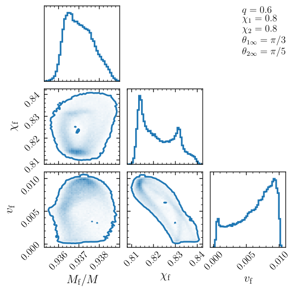
We start by considering a single binary at $r/M\to\infty$ and studying the impact of the two phases. In the examples below we selected a source with $q=0.6$, $\chi_{1}=\chi_{2}=0.8$, $\theta_{1\infty}=\pi/3$, and $\theta_{2\infty}=\pi/5$ but the trends we highlight are generic.

We first evolve this same binary $10^{5}$ times repeatedly sampling over all three sources of uncertainty: the precessional phase $S_{\mathrm{pre\to orb}}$, the orbital phase $\varphi_{\mathrm{orb\to sur}}$, and the surrogate Gaussian errors. Figure 2 shows the resulting distribution of the BH remnant properties. GWs dissipate energy and angular momentum relatively gradually during the inspiral; on the other hand, the vast majority of the linear momentum is emitted during the last few orbits and plunge [30, 31]. The exact configuration with which the binary approaches merger, therefore, plays a more crucial role for $v_{\rm f}$ compared to $M_{\rm f}$ and $\chi_{\rm f}$. For this specific binary, the final mass presents a median value of $M_{\rm f}\simeq 0.937M$ with a dispersion $\delta M_{\rm f}\simeq 0.1\%$. The final spin presents uncertainties that are up to an order of magnitude larger: the 90% confidence interval extends for about $\delta\chi_{\rm f}\simeq 1.4\%$ from a median value $\chi_{\rm f}\simeq 0.82$. The kick is subject to variations which are even more extreme: possible values of the final recoil range from $v_{\rm f}\mathchar 21016\,0$ to $\mathchar 21016\,0.01$.

We now dissect the various contributions entering these uncertainties.

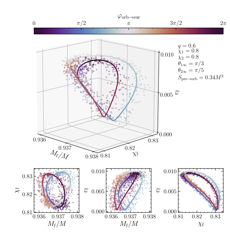
Figure 3 shows the remnant properties of the same asymptotic configuration considered previously, but now assuming a fixed value of the precessional phase $S_{\rm pre\to orb}=0.34M^{2}$. We then vary $\varphi_{\rm orb\to sur}$ from $0$ to $2\pi$. The solid curves in Fig. 3 show the median values $\overline{M}_{\mathrm{f}}$, $\overline{\chi}_{\mathrm{f}}$ and $\overline{v}_{\mathrm{f}}$ returned by the NR surrogate; circles mark a sample of remnants extracted from the corresponding Gaussian distributions.

The orbital-phase uncertainty on the remnant properties is due to the breaking down of the PN timescale hierarchy. The series of binaries depicted in Fig. 3 is computed for different phases $\varphi_{\mathrm{orb\to sur}}$ and fixed orbital frequency $\omega_{\rm orb\to sur}$. For $t_{\rm orb}/t_{\rm pre}\to 0$ and $t_{\rm orb}/t_{\rm RR}\to 0$, this sequence is equivalent to the same binary moved along a quasi-adiabatic orbit, and should just result in identical remnants. Deviations from these limits imply that, although these sources are identical up to $r_{\rm pre\to orb}$, they evolve into different configurations and thus result in different merger remnants.

By construction, the curve describing the surrogate median values is periodic as $\varphi_{\mathrm{orb\to sur}}$ ranges from $0$ to $2\pi$. An approximate periodicity with period equal to $\pi$ is also present, such that the curve in Fig. 3 appears as two, largely overlapping loops. A period equal to twice the orbital frequency corresponds to that of the dominant GW emission. The separation between the two loops is typically smaller than the Gaussian errors of the surrogate model, and thus largely disappears when these are considered (scatter points).

For binaries with $q=1$ and $\mathbf{S_{1}}=\mathbf{S_{2}}$, a transformation $\varphi\to\varphi+\pi$ can be absorbed into a change of reference frame and thus results in identical values of $M_{\rm f}$, $\chi_{\rm f}$, and $v_{\rm f}$. The two-loop structure of Fig. 3 thus collapses into a single loop (in practice, this is only true within the errors of the surrogate model because this expected symmetry was not built in explicitly in Ref. [38]). For non-symmetric binaries, the $\pi$ periodicity is broken resulting in a more complex phenomenology. In general, we find that for binaries with more extreme mass ratios $q\lesssim 0.25$, the loop of the median values becomes tighter and is eventually “filled” as the surrogate errors are considered. We refer to Refs. [45, 46] for a careful analysis of the expected symmetries.

Figure 4 shows how the remnant properties vary with the precessional phase $S_{\rm pre\to orb}$. While the precise shape of the curves depends on the sampled value, the general behavior we described remains valid: the remnant properties present an approximate period equal to that of the dominant GW mode, which is half the orbital period. The region covered by the loops mildly changes with $S$, such that the weighted superpositions of all the loops in Fig. 4 returns the full distribution we first showed in Fig 2. Each individual contribution is weighted by the probability density function $p(S)\propto|dS/dt|^{-1}$, which is strongly peaked at the two extrema $S_{-}$ and $S_{+}$ [41]. The loops with the larger and smaller values of $S_{\rm pre\to orb}$ (top and bottom row in Fig. 4) provide the largest contributions to the overall distribution and can indeed be glimpsed when carefully inspecting Fig. 2. The bimodality observed in the marginalized distributions on Fig. 2 is also a direct consequence of this loop structure.

We now consider BH binary populations and investigate the statistical properties of their remnants.

In Fig. 5, we focus on a population with fixed $q=0.8$ and $\chi_{1}=0.6$ and $\chi_{2}=0.7$. First, we map the entire $(\cos\theta_{\rm 1\infty},\cos\theta_{\rm 2\infty})$ plane into the $(M_{\rm f},\chi_{\rm f})$ parameter space (gray region in the right panel of Fig. 5). Final mass and final spin are strongly anti-correlated, with large values of $M_{\rm f}$ corresponding to small values of $\chi_{\rm f}$, and vice-versa. This is due to the orbital hang-up effect [39, 47, 48]. Binaries with spins which are both aligned to the orbital angular momentum ($\theta_{1\infty}\simeq\theta_{2\infty}\simeq 0$, corresponding to larger positive values of $\xi$ in the upper right corner of the left panel of Fig. 5) inspiral for longer: they dissipate more energy via GWs and result in lighter remnant. Their angular momenta add constructively ($|\mathbf{L}+\mathbf{S_{1}}+\mathbf{S_{2}}|\simeq L+S_{1}+S_{2}$) resulting in a larger final spin. On the contrary, binary with spins which are largely anti-aligned plunge from afar but the spins and angular momentum partially cancel each other, thus producing remnants which are heavier and more slowly rotating.

We then consider a subsample of 25 equispaced sources from the same population, shown as coloured dots in the left panel of Fig. 5. In particular, binaries are coloured according to the projected effective spin $\xi$ [Eq. (2)]. We evolve each of these systems $10^{4}$ times, sampling over $S_{\mathrm{pre\to orb}}$, $\varphi_{\mathrm{orb\to sur}}$ and the surrogate Gaussian errors. The corresponding distributions in the remnant parameter space are shown in the right panel of Fig. 5 with the same color scheme. The larger these regions, the more uncertain the remnant properties are. The size of the regions correlates with $\xi$: remnant uncertainties tend to be larger for $|\xi|\mathchar 21016\,0$ and smaller for values at the extrema $|\xi|\mathchar 21016\,(\chi_{1}+q\chi_{2})/(1+q)$. This is because the former systems have larger precessional amplitudes $|S_{+}-S_{-}|$ while for the latter the range where $S_{\mathrm{pre\to orb}}$ can be sampled is more limited [35].

Figure 6 shows the uncertainties on the remnant properties for a wider set of BH binary populations. In particular, we consider three cases with fixed values $q=0.6$ and $\chi_{1}=\chi_{2}=0.3$, $q=0.6$ and $\chi_{1}=\chi_{2}=0.8$, $q=0.95$ and $\chi_{1}=\chi_{2}=0.8$, as well as a fourth scenario where we distribute the mass ratio according to $p(q)\propto q^{6.7}$ in $[0.25,1]$ and the spin magnitudes uniformly in $[0.1,0.8]$. The latter is motivated by current GW detections which favour equal-mass systems [49] (but see Ref. [10]). In all four cases, we consider both isotropically distributed spins (top panels) and partially aligned spins (bottom panels) at past time infinity, which correspond to distributing $\cos\theta_{i\infty}$ either uniformly in $[-1,1]$ or with a truncated normal distribution centered on 1 with dispersion 0.1, respectively. We extract 1000 samples from each of these populations. These asymptotic configurations are then evolved 1000 times, sampling the precessional and orbital phases, to obtain corresponding distributions of the remnant properties. We then construct the estimators $\delta M_{\rm f}$, $\delta\chi_{\rm f}$ and $\delta v_{\rm f}$ of Eq. (11) which are shown in Fig. 6.

Uncertainties on $M_{\rm f}$ and $\chi_{\rm f}$ tend to be smaller for populations where a large fraction of the binaries possess either (i) mass ratio $q$ close to unity, (ii) small magnitudes $\chi_{i}$, or (iii) small spin misalignments $\theta_{i\infty}$. Binaries with $q\to 1$ result in more similar remnants because the spin magnitude $S$ asymptotes to a constant [50]. Systems with either $q\to 0$, $\chi_{i}\to 0$, or $\theta_{i\infty}\to 0$ are all well described by a single-spin approximation [33, 51] where $S$ is also approximately constant. Precession effects are less important for the distribution of $v_{\rm f}$ because the contribution of the orbital-phase sampling is more dominant. In general, for the populations studied here we find $\delta M_{\rm f}\lesssim 0.004$, $\delta\chi_{\rm f}\lesssim 0.03$, and $\delta v_{\rm f}\lesssim 1.5$.

We now exploit our evolutionary procedure to highlight correlations between the remnant properties and the precessional dynamics at small separations. We make use of the concept of spin morphology [35, 34, 50, 52, 53]. The dynamics of BH binaries can be unambiguously classified into three different classes according to the qualitative behavior of the spin angle $\Delta\Phi$ [Eq. (2)]. In particular, $\Delta\Phi$ can either librate about $0$ and never reach $\pm\pi$ (L0), circulate through the full range $[-\pi,\pi]$ (C), or librate about $\pm\pi$ and never reach $0$ (L$\pi$). All binaries belong to the circulating morphology at large separation, but GW radiation reaction will generically cause transitions towards the two librating classes before merger. In the following, we correlate the properties of the merger remnant to the spin morphology evaluated at $\omega_{\rm orb\to sur}$, i.e. right before initializing the NR surrogate.

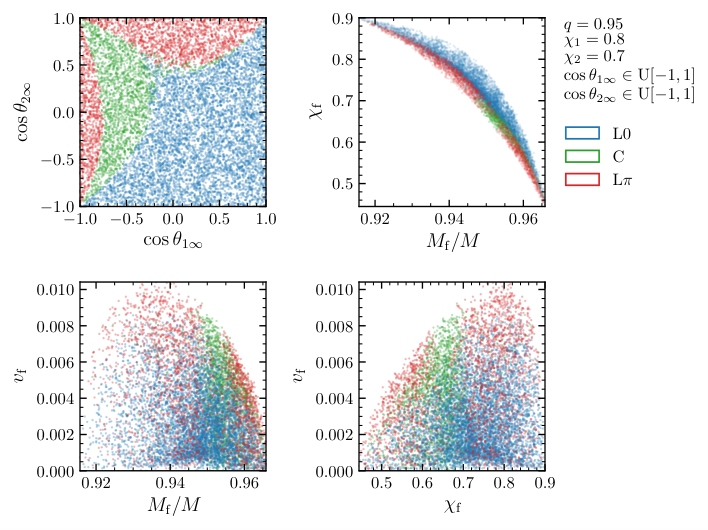
The spin morphology before merger provides a useful mapping between the two asymptotic configurations of the evolution – the large-separation limit and the post-merger remnant. In Fig. 7 we illustrate this point showing a population of $10^{5}$ sources with $q=0.95$, $\chi_{1}=0.8$, $\chi_{2}=0.7$, and isotropic spin directions at large separations. Binaries in each each of the three morphologies tend to cluster in well defined regions of both the ($\theta_{1\infty},\theta_{2\infty}$) and the remnant parameter spaces.⁴⁴ 4 For fixed $q$, $\chi_{1}$, $\chi_{2}$, and $r$, the morphology separation in the ($\theta_{1\infty},\theta_{2\infty}$) plane is exact [35]. In this case, we are evaluating the morphology at fixed orbital frequency $\omega_{\rm orb\to sur}$ which causes minor overlaps between the different classes. If $\Delta\Phi$ librates about $0$ ($\pi$), in-plane spin components are closer to alignment (anti-alignment) with each other and produce, on average, final BHs with masses and spins which are above (below) the hang-up anti-correlation (top-right panel of Fig. 7)

In the left panel of Fig 8, we consider the same population and focus on the distributions of the recoil velocities. We find that $\mathchar 21016\,35$% ($\mathchar 21016\,100$%) of the binaries with $v_{\rm f}\geq 1000$ km/s (3000 km/s) belong to the $\Delta\Phi\sim\pi$ morphology before merger. This can be also be seen in bottom panels of Fig. 7, where red points preferentially populate the regions with large values of $v_{\rm f}$. The role of the spin morphology can be traced back to the very first “superkick” NR simulations [54, 55] where BHs were initialized with $|\Delta\Phi|=\pi$ and $\theta_{i}=\pi/2$. In this setup, frame dragging of the the two BHs can act constructively, boosting the recoil [30]. Binaries with $|\Delta\Phi|=\pi$ and partial alignment $\theta_{i}\lesssim\pi/2$ result in even larger recoils because more energy is emitted [56]. Conversely, binaries which librate about $\Delta\Phi=0$ before merger present lower kicks of $\mathcal{O}(100)$ km/s and are responsible for the bulk of the population. Circulating sources present a rather flat distribution and allow for most values of $v_{\rm f}$ but the largest ones.

In the right panel of Fig 8, we repeat the same exercise but assume a mass ratio distribution $p(q)\propto q^{6.7}$ [49] with $q\in[0.25,1]$ and uniform spin magnitudes $\chi_{i}\in[0.1,0.8]$. Compared to the previous case, BHs have, on average, lower spins which implies weaker recoils [57] and a larger fraction of circulating binaries [35]. The general trends we highlighted above remain valid: the largest (smallest) kicks are largely due to binaries which were librating about $\Delta\Phi=\pi$ ($\Delta\Phi=0$) before merger.

Finally, we investigate the robustness of our approach with respect to the two transition thresholds $r_{\rm pre\to orb}$ and $\omega_{\rm orb\to sur}$. Figure 9 shows how median and $90\%$ interval of the three remnant quantities vary for a population of 1000 binaries with $q$ uniformly distributed in $[0.25,1]$, $\chi_{i}$ uniformly distributed in $[0.1,0.8]$, and isotropic spin directions $\theta_{\rm i\infty}$. We evolve each source 1000 times, sampling over $S_{\mathrm{pre\to orb}}$, $\varphi_{\mathrm{orb\to sur}}$ and the surrogate Gaussian errors, and report the 90% interval of the remnant properties (Fig. 9). We do this for 100 values of $r_{\rm pre\to orb}$ spread evenly in $[50M,3000M]$ with fixed $\omega_{\mathrm{orb\to sur}}=0.025\,\mathrm{rad}/M$, and for 100 values of $\omega_{\mathrm{orb\to sur}}$ spread evenly in $[0.02\,\mathrm{rad}/M,0.03\,\mathrm{rad}/M]$ with fixed $r_{\rm pre\to orb}=1000M$. The remnant population does not depend sensibly on either of the thresholds in these ranges, though we observe greater discrepancies in $v_{\mathrm{f}}$ than the other remnant properties.

We also show five random sources from the same population (gray curves in Fig. 9). The median levels of the remnant mass and spin do not depend strongly on the threshold values, though greater cyclic variation is present in the median levels of the remnant kick velocity. Over the full population this variation is not significant compared to the reported dispersion.

References

- [1] Abbott B P et al. (LIGO and Virgo Collaboration) 2019 PRX 9 031040 [arXiv:1811.12907]
- [2] Venumadhav T, Zackay B, Roulet J, Dai L and Zaldarriaga M 2020 PRD 101 083030 [arXiv:1904.07214]
- [3] Nitz A H, Dent T, Davies G S, Kumar S, Capano C D, Harry I, Mozzon S, Nuttall L, Lundgren A and Tápai M 2020 APJ 891 123 [arXiv:1910.05331]
- [4] Gravitational-wave candidate event database, LIGO/Virgo O3 public alerts gracedb.ligo.org/superevents/public/O3
- [5] Akutsu T et al. (KAGRA Collaboration) 2017 [arXiv:1710.04823]
- [6] Unnikrishnan C S 2013 IJMPD 22 1341010 [arXiv:1510.06059]
- [7] Amaro-Seoane P et al. (LISA Core Team) 2017 [arXiv:1702.00786]
- [8] Abbott B P et al. (LIGO and Virgo Collaboration) 2016 PRL 116 241103 [arXiv:1606.04855]
- [9] Chatziioannou K et al. 2019 PRD 100 104015 [arXiv:1903.06742]
- [10] Abbott B P et al. (LIGO and Virgo Collaboration) 2020 [arXiv:2004.08342]
- [11] Zackay B, Venumadhav T, Dai L, Roulet J and Zaldarriaga M 2019 PRD 100 023007 [arXiv:1902.10331]
- [12] Apostolatos T A, Cutler C, Sussman G J and Thorne K S 1994 PRD 49 6274–6297
- [13] Peters P C and Mathews J 1963 Physical Review 131 435–440
- [14] Bekenstein J D 1973 APJ 183 657–664
- [15] Gerosa D, Kesden M, Berti E, O’Shaughnessy R and Sperhake U 2013 PRD 87 104028 [arXiv:1302.4442]
- [16] Stevenson S, Berry C P L and Mandel I 2017 MNRAS 471 2801–2811 [arXiv:1703.06873]
- [17] Vitale S, Lynch R, Sturani R and Graff P 2017 CQG 34 03LT01 [arXiv:1503.04307]
- [18] Talbot C and Thrane E 2017 PRD 96 023012 [arXiv:1704.08370]
- [19] Farr W M, Stevenson S, Miller M C, Mandel I, Farr B and Vecchio A 2017 Nature 548 426–429 [arXiv:1706.01385]
- [20] Farr B, Holz D E and Farr W M 2018 APJL 854 L9 [arXiv:1709.07896]
- [21] Gerosa D, Berti E, O’Shaughnessy R, Belczynski K, Kesden M, Wysocki D and Gladysz W 2018 PRD 98 084036 [arXiv:1808.02491]
- [22] Rodriguez C L, Zevin M, Pankow C, Kalogera V and Rasio F A 2016 APJL 832 L2 [arXiv:1609.05916]
- [23] Antonini F, Rodriguez C L, Petrovich C and Fischer C L 2018 MNRAS 480 L58–L62 [arXiv:1711.07142]
- [24] McKernan B, Ford K E S, O’Shaugnessy R and Wysocki D 2020 MNRAS 494 1203–1216 [arXiv:1907.04356]
- [25] Berti E and Volonteri M 2008 APJ 684 822–828 [arXiv:0802.0025]
- [26] Sesana A, Barausse E, Dotti M and Rossi E M 2014 APJ 794 104 [arXiv:1402.7088]
- [27] Gerosa D, Veronesi B, Lodato G and Rosotti G 2015 MNRAS 451 3941–3954 [arXiv:1503.06807]
- [28] Kesden M, Sperhake U and Berti E 2010 PRD 81 084054 [arXiv:1002.2643]
- [29] Kesden M, Sperhake U and Berti E 2010 APJ 715 1006–1011 [arXiv:1003.4993]
- [30] Brügmann B, González J A, Hannam M, Husa S and Sperhake U 2008 PRD 77 124047 [arXiv:0707.0135]
- [31] Gerosa D, Hébert F and Stein L C 2018 PRD 97 104049 [arXiv:1802.04276]
- [32] Schnittman J D 2004 PRD 70 124020 [arXiv:astro-ph/0409174]
- [33] Racine É 2008 PRD 78 044021 [arXiv:0803.1820]
- [34] Kesden M, Gerosa D, O’Shaughnessy R, Berti E and Sperhake U 2015 PRL 114 081103 [arXiv:1411.0674]
- [35] Gerosa D, Kesden M, Sperhake U, Berti E and O’Shaughnessy R 2015 PRD 92 064016 [arXiv:1506.03492]
- [36] Blackman J, Field S E, Scheel M A, Galley C R, Ott C D, Boyle M, Kidder L E, Pfeiffer H P and Szilágyi B 2017 PRD 96 024058 [arXiv:1705.07089]
- [37] Varma V, Gerosa D, Stein L C, Hébert F and Zhang H 2019 PRL 122 011101 [arXiv:1809.09125]
- [38] Varma V, Field S E, Scheel M A, Blackman J, Gerosa D, Stein L C, Kidder L E and Pfeiffer H P 2019 Physical Review Research 1 033015 [arXiv:1905.09300]
- [39] Damour T 2001 PRD 64 124013 [arXiv:gr-qc/0103018]
- [40] Chatziioannou K, Klein A, Yunes N and Cornish N 2017 PRD 95 104004 [arXiv:1703.03967]
- [41] Gerosa D and Kesden M 2016 PRD 93 124066 [arXiv:1605.01067]
- [42] Varma V, Isi M and Biscoveanu S 2020 PRL 124 101104 [arXiv:2002.00296]
- [43] Kidder L E 1995 PRD 52 821–847 [arXiv:gr-qc/9506022]
- [44] Rasmussen C E and Williams C K I 2006 Gaussian Processes for Machine Learning (MIT press)
- [45] Boyle L, Kesden M and Nissanke S 2008 PRL 100 151101 [arXiv:0709.0299]
- [46] Boyle L and Kesden M 2008 PRD 78 024017 [arXiv:0712.2819]
- [47] Campanelli M, Lousto C O and Zlochower Y 2006 PRD 74 041501 [arXiv:gr-qc/0604012]
- [48] Scheel M A, Giesler M, Hemberger D A, Lovelace G, Kuper K, Boyle M, Szilágyi B and Kidder L E 2015 CQG 32 105009 [arXiv:1412.1803]
- [49] Abbott B P et al. (LIGO and Virgo Collaboration) 2019 APJL 882 L24 [arXiv:1811.12940]
- [50] Gerosa D, Sperhake U and Vošmera J 2017 CQG 34 064004 [arXiv:1612.05263]
- [51] Schmidt P, Ohme F and Hannam M 2015 PRD 91 024043 [arXiv:1408.1810]
- [52] Gerosa D, Lima A, Berti E, Sperhake U, Kesden M and O’Shaughnessy R 2019 CQG 36 105003 [arXiv:1811.05979]
- [53] Phukon K S, Gupta A, Bose S and Jain P 2019 PRD 100 124008 [arXiv:1904.03985]
- [54] González J A, Hannam M, Sperhake U, Brügmann B and Husa S 2007 PRL 98 231101 [arXiv:gr-qc/0702052]
- [55] Campanelli M, Lousto C O, Zlochower Y and Merritt D 2007 PRL 98 231102 [arXiv:gr-qc/0702133]
- [56] Lousto C O and Zlochower Y 2011 PRL 107 231102 [arXiv:1108.2009]
- [57] Lousto C O, Zlochower Y, Dotti M and Volonteri M 2012 PRD 85 084015 [arXiv:1201.1923]
- [58] Ghosh A, Ghosh A, Johnson-McDaniel N K, Mishra C K, Ajith P, Del Pozzo W, Nichols D A, Chen Y, Nielsen A B, Berry C P L and London L 2016 PRD 94 021101 [arXiv:1602.02453]
- [59] Gerosa D and Moore C J 2016 PRL 117 011101 [arXiv:1606.04226]
- [60] Arca Sedda M and Benacquista M 2019 MNRAS 482 2991–3010 [arXiv:1806.01285]
- [61] De Luca V, Franciolini G, Pani P and Riotto A 2020 JCAP 2020 052 [arXiv:2003.02778]