Fluctuation-theorem and extended thermodynamics of turbulence
Abstract
Turbulent flows are out-of-equilibrium because the energy supply at large scales and its dissipation by viscosity at small scales create a net transfer of energy among all scales. Here, the energy cascade is approximated by a combined contribution of a forward drift and diffusion that recover accepted phenomenological theories of turbulence. The fluctuation theorem (FT) is then shown to describe the scale-wise statistics of forward and backward energy transfer and their connection to irreversibility and entropy production. The ensuing turbulence entropy may be used to formulate an extended turbulence thermodynamics.
I Introduction
It is perhaps not coincidental that one of the most influential experiments in the history of thermodynamics is also a turbulence experiment. In 1849, James Prescott Joule used a stirrer to show that the shaft work on a fluid ends up increasing its internal energy, thereby demonstrating the equivalence of heat and work. Dealing with the generation of turbulent kinetic energy () and its subsequent dissipation rate () by viscosity, the Joule experiment also offers a modern link between thermodynamics, a theory of the macroscopic effects of microscopic fluctuations, and non-equilibrium fluctuations, of which turbulence is a quintessential example. On the one hand, the disparity between microscopic and macroscopic fluctuations appears un-reconcilable. Thermodynamic fluctuations are so small to allow a mathematical description of fluids as a continuum. For this reason, turbulence is conveniently described by the Navier-Stokes equations assuming local thermodynamic equilibrium (Panton 2006). Turbulent fluctuations are thus of macroscopic nature and technically outside the scope of traditional thermodynamics (Sreenivasan 1999). On the other hand, the random-like nature of turbulence (Batchelor 1953; Monin and Yaglom 1975; Hinze 1959) invites a thermodynamic formalism to the problem of turbulence, including the eddy thermodynamics of Richardson (Richardson 1920), Blackadar (Blackadar 1955) and others (Nevzglyadov 1961; Reinke et al. 2018), as well as the Onsager analysis of 2D turbulence (Eyink and Sreenivasan 2006). Liepmann 1979 asserted that ‘turbulence can be defined by a statement of impotence reminiscent of the second law of thermodynamics’. More recently, a number of studies have argued that the fluctuation theorem derived for small systems (Evans and Searles 2002; Gallavotti and Cohen 1995) can be partly applied to describe macroscopic fluctuations so as to explore their time reversibility at multiple scales, including turbulence.
The statistical properties of turbulence differ from systems near thermal equilibrium because the flux of energy per unit mass is supplied at scales much larger than the scales at which energy is dissipated by the action of viscosity, resulting in an energy flux (cascade) across all scales. Such a transport is linked to multiple processes, including vortex stretching, self-amplification of the strain-rate and viscous diffusion (Tennekes et al. 1972; Carbone and Bragg 2020). One of the defining features of the turbulence cascade is that the probability of forward and backward transitions between two energetic states at a given scale are not identical (i.e., a scale-wise ‘detailed balance’ is not applicable (Xu et al. 2014; Fuchs et al. 2020)).
The objective of this work is to illustrate that non-equilibrium thermodynamics, and in particular, the fluctuation theorem can be extended to describe the behavior of the turbulent energy cascade. While the net transfer of energy from large to small scales is prevalent, it is shown here that back-scatter of energy and its connection to time-scale irreversibility obeys the statistics predicted by the fluctuation theorem (Evans et al. 1993; Gallavotti and Cohen 1995; Porporato et al. 2007; Zorzetto et al. 2018; Fuchs et al. 2020). To provide a physical context, a turbulent flow conceptually analogous to Joule’s original experiment is used, where work is done on the fluid system to generate in a narrow band of scales, which is then dissipated as heat thereby raising the internal energy. In the analysis here, constant energy is externally supplied at a pre-selected scale much larger than the Kolmogorov length scale () where viscous effects are significant. At steady state, the energy cascade develops in a manner where the energy injection rate is balanced by viscous dissipation rate as in Joule’s experiment. The fluctuation theorem is then applied to describe the forward and backward probabilities of energy packets moving scale-wise in time through the energy cascade. For analytical tractability and to illustrate connections with the fluctuation theorem, simplified closure schemes for the energy transfer rate across scales are employed. These closure schemes offer plausible expressions for the energy cascade that are consistent with a wide range of experiments and theories on locally homogeneous and isotropic turbulence.
II Spectral Energy Balance
For a homogeneous, isotropic turbulent flow of a Newtonian, incompressible viscous fluid, the spectral energy balance per unit mass of fluid is (Batchelor 1953; Panchev 1971; Monin and Yaglom 1975)
| (1) |
where is the turbulent kinetic energy per unit wave number , is the production spectrum here assumed to be concentrated at , is the energy transfer spectrum, is the viscous dissipation spectrum, and is the wavenumber or inverse eddy-size. The normalizing property defines the turbulent kinetic energy . Eq. (1) makes no other assumptions about the velocity statistics other than homogeneity and isotropy. Because is a scale-wise transport and cannot contribute to production or destruction of , it satisfies the integral constraint . It can be expressed as the gradient of an energy flux ,
| (2) |
while the scale-wise viscous dissipation rate is given by
| (3) |
Integrating Eq. (1) over yields the energy balance of ,
| (4) |
where is the rate of work done on the fluid to produce turbulence and is the dissipation rate of ,
| (5) |
The concomitant balance for internal energy is then , where is the heat loss to the environment. Because of fluid incompressibility, temperature fluctuations resulting from dissipation have no feedback on the dynamics of the turbulence, including the energy cascade. Finally, the entropy balance is given by , where is the absolute temperature and is the entropy production. It is assumed that is immediately delivered to a surrounding environment, acting as a thermal bath at the same temperature, thus ensuring isothermal conditions.
Returning to the spectral energy balance, a closure of minimal complexity that preserves both direct energy cascade and an inverse cascade (or backscatter) may be obtained by representing the contributions to as scale-wise drift and a diffusion term linked by a timescale of eddy relaxation . A flexible form for such a closure is proposed here as
| (6) |
where the coefficient is to be determined depending on models for (Onsager 1949; Corrsin 1964; Danaila and Antonia 2009; Poggi et al. 2011). Substituting and from Eqs. (6) and (3) into the spectral energy balance in Eq. (1) yields
| (7) |
Depending on the choices made about , a general class of non-linear diffusion models for can be recovered. Here, a that is linked to is adopted,
| (8) |
For the inertial subrange scales, the Kolmogorov (Kolmogorov 1941) scaling (hereafter referred to as K41 scaling) given by is expected to hold resulting in (i.e. Onsager’s relaxation time (Eyink and Sreenivasan 2006)), where is the Kolmogorov constant. Due to the dissipative anomaly (Falkovich et al. 2001), is finite, so that in this limit , . We may then estimate the total time for energy to be passed from a finite to an infinitely high wavenumber by
| (9) |
Eq. (9) implies that the steps in the energy cascade rapidly accelerate such that (if not interrupted by the action of viscosity at a finite wavenumber) the time for energy to be passed to an infinitely high wavenumber is finite. This finding, originally put forth by Onsager (Eyink and Sreenivasan 2006), foreshadows the finite time singularity in the inviscid limit for such classes of models (Davidson 2015). The in (8) is also singled out because it recovers the well-studied Leith’s non-linear diffusion approximation (Leith 1968; Besnard et al. 1996; Clark et al. 2009),
| (10) |
When , the conventional form of Leith’s model becomes evident (Leith 1968; Panchev 1971). The latter recovers the so-called warm cascade condition (i.e. a steady equipartitioned energy spectrum, ) originally derived by Lee (Lee 1952) under specific conditions (Besnard et al. 1996; Connaughton and Nazarenko 2004; Clark et al. 2009). Leith’s model was also derived from the so-called direct-interaction approximation when a number of simplifications are made (Clark et al. 2009).
For stationary conditions, and far from the production and viscous subranges, , the solution to the spectral budget reduces to
| (11) |
If is injected at , then for necessitating to recover K41 inertial subrange scaling (also referred to as the cold cascade). For , and is set by the continuity of at to achieve a warm cascade for (Connaughton and Nazarenko 2004). The is also compatible with the well-known Saffman spectrum (Saffman 1967; Meyers and Meneveau 2008; Davidson 2015), a scaling law derived from considerations (continuity and smoothness) of how is approached as .
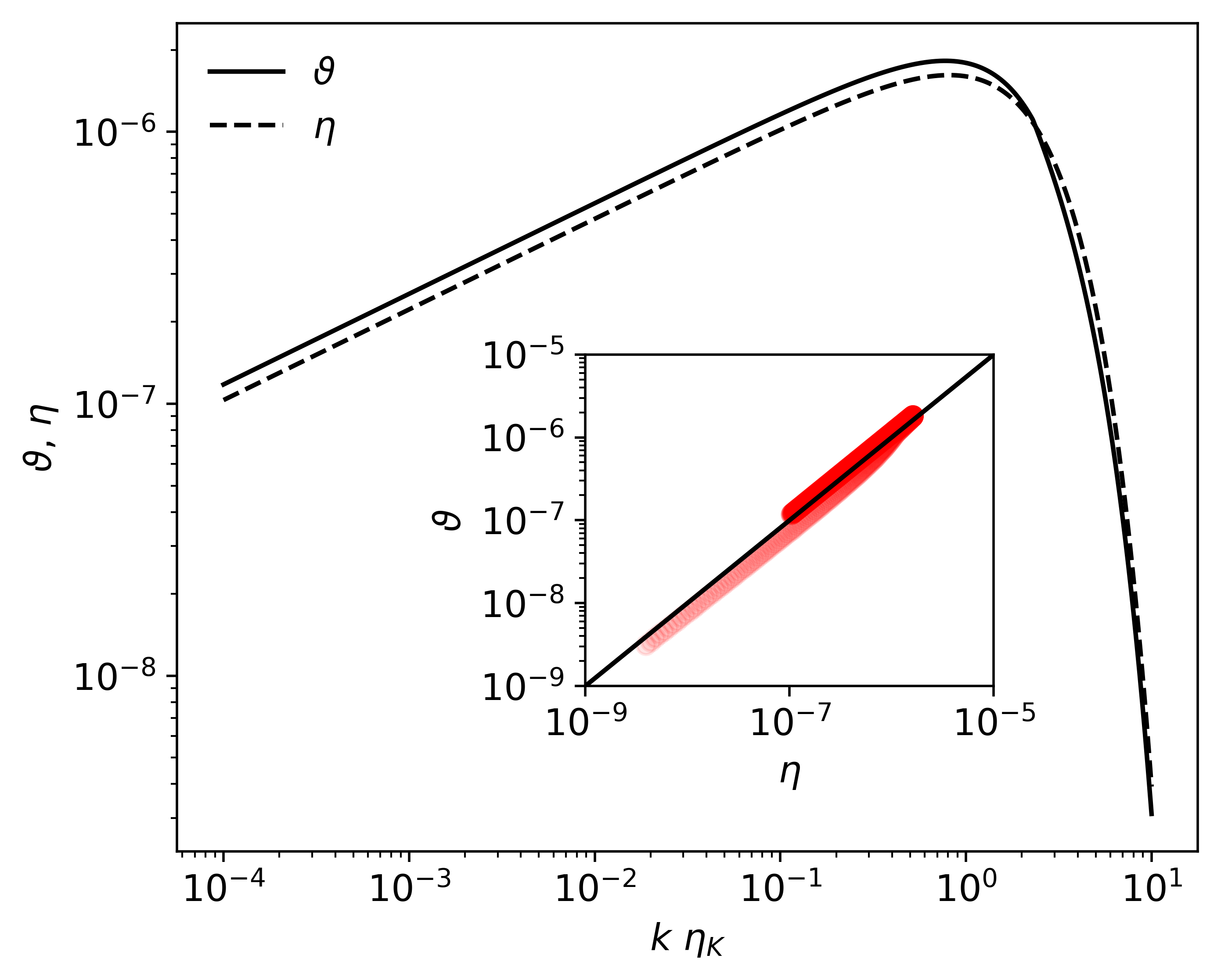
In the presence of viscous dissipation, the spectral budget equation is not analytically solvable, however, we numerically confirm that
| (12) |
reasonably approximates the spectral energy budget, as shown in Fig 1. Here, is the Pao correction (Pao 1965) reshaping the spectrum for (Lamorgese et al. 2005). The from Eq. (12) implies that in Eq. (8) increases within the viscous sub-range when , which is not physically plausible. The increase in is expected when decreases faster than with increasing . Hence, an amendment proposed by Batchelor (Batchelor 1959) was used in the calculations featured in Fig 1 whereby the straining rate () at is assumed to be uniform beyond scales commensurate with . This amendment revises the model for as
| (13) |
where is the Kolmogorov time scale.
III Fluctuation Theorem
The spectral budget in Eq. (7) can be interpreted as a nonlinear Fokker-Planck equation (FPE) with scalewise separated source/sink terms. Accordingly, the underlying cascade can be expressed as a stochastic process (Gardiner 1994), whereby trajectories represent time histories of energy packets (eddies) traveling in -space driven by advection and diffusion, until they disappear by virtue of a killing term linked to the action of viscous dissipation. The latter term absorbs trajectories as a state-dependent Poisson process with a rate Daly and Porporato 2007.
If the steady-state solution is known (Eq. 12), the corresponding drift and diffusion for the position in space of the energy packet can be formulated as a function of . Thus, a Langevin equation that ensures that the steady-state probability density function (PDF) abides by Eq. (12) is
| (14) |
where is the Wiener increment and . This equation is subjected to a unit rate of birth at and a state dependent killing term with rate (Daly and Porporato 2007). Since the FPE is written in the so-called transport form, the interpretation of the multiplicative term is the one of Hanggi-Klimontovich (Hanggi 1978; Klimontovich 1990; Porporato et al. 2011).
With this formal correspondence, the statistics of irreversiblity of Eq. (14) can now be analyzed (Porporato et al. 2007; Porporato et al. 2011) for steady-state homogeneous and isotropic turbulence with energy injected at and transported on average towards higher wavenumbers where dissipation takes place. This allows an illustration of the fluctuation theorem for fully developed turbulence fluctuations, linking the turbulent entropy balance at to those of forward and backward energy cascades. Fig 2a shows a numerical realization of this process in which energy packets are injected at after the termination of trajectories by dissipation. While the energy injection at is only related statistically to the dissipation, the immediate re-injection after killing adopted here for convenience of simulation and visualization preserves the steady state PDF. As shown in Fig 2b, the steady state PDF of the time series corresponds to the empirical spectrum in Eq. (12).

The injection of energy at lower and the dissipation sink at higher produce a non-zero average current and a non-equilibrium steady state (NESS) current of energy towards smaller scales. The stochastic fluctuating velocity is a random variable with mean current velocity given by (Porporato et al. 2011)
| (15) |
and a fundamental FT-type symmetry (Porporato et al. 2007). The degree of irreversibility of the NESS resulting from the cascade towards dissipation may be given by the rate of energy transfer to smaller scales. According to the formalism of stochastic thermodynamics (Seifert 2012; Jarzynski 2011), the non-zero current velocity may be associated with a positive ‘turbulent entropy’ production rate (Porporato et al. 2011),
| (16) |
IV An Extended Turbulence Thermodynamics
The term can be shown to be the source term in the balance equation for the turbulent entropy Seifert 2005. In this view, the asymmetry in the turbulence cascade that not only transports energy forward to higher wave numbers (the forward turbulence cascade) but also backward (the so-called back scatter) contributing energy to larger eddies, is also linked to a turbulent entropy production. Specifically, if one considers the (random) path of a turbulent energy packet over a period of time , the ensemble average of the ratio of the path measures between forward and backward cascade, that is the path measures the forward and backward PDFs of evaluated along stochastic trajectories that take place on a common interval in steady state conditions Maes and Netočnỳ 2003; Porporato et al. 2011, is
| (17) |
Thus, can be interpreted as a scale-wise ‘turbulence entropy’, which together with TKE may be used to define an extended turbulence thermodynamics as in Richardson’s (Richardson 1920), providing a measure of the number of turbulent states at wave number to be linked to the corresponding portion of TKE. Neglecting momentarily the viscous subrange, TKE can be linked to the area under the spectrum given in Eq. (11), namely
| (18) |
where is a Reynolds number formed from a characteristic length and velocity . This definition ensures that consistent with expectations for many turbulent flows (Tennekes et al. 1972). The integrated entropy can also be obtained as
| (19) |
One objection that can be raised here is that is not an entropy in the sense of Clausius, but an extended entropy related to macroscopic turbulent fluctuations. However, similar to classical thermodynamics, we may consider the TKE to correspond to an internal kinetic energy of turbulence, so that , analogous to an effective temperature for the turbulent system. When such a definition is combined with Eq 18, the extended turbulence thermodynamics can proceed as follows:
| (20) |
An integrated positive turbulence-entropy production for the integrated turbulence entropy, , can be readily obtained assuming that molecular dissipation primarily acts in the neighborhood of . For where and , and . As a result,
| (21) |
In the limit of high the above relationships approach to , , , and , where and are deviations due to the logarithmic terms. At Re , the spectrum within the inertial subrange vanishes with production scales being commensurate to the Kolmogorov microscale (). For this case, (detailed balance holds) although the cascade still generates small , , and . The key quantities in this turbulent thermodynamics are plotted in Fig. 3. The fundamental equation, shows a downward concavity that ensures entropy production by ‘combining’ turbulent flows of different TKE, while the dependence of on shows a turbulent TKE capacity () that is not constant but decays with the Reynolds number.

V Conclusions
The fluctuation theorem has been used to analytically link the shape of the energy spectrum with the imbalance between forward and backward probabilities of energy packets moving scale-wise in time across the energy cascade. The difference between these two aforementioned probabilities is the main cause why the ‘detailed balance’ or ‘microscopic reversibility’ (i.e. at equilibrium, each elementary process is in equilibrium with its reverse process) is not applicable to turbulence, and why turbulent fluctuations are presumed to be far from equilibrium.
The previous result unfolded a connection between the turbulent entropy production rate measuring the effective spreading of energy-packet trajectories in the cascade, the thermodynamic entropy production, and the Reynolds number for an externally prescribed injection scale (often dictated by boundary conditions or geometry). As first pointed out by Landau (Landau and Lifshitz 1959) and substantiated in later studies (Constantin et al. 1985), the finite is an indicator of the number of degrees of freedom of the turbulence cascade, .
An additional foresight from this analysis is that the shape of the spectrum at low . It is shown here that the Saffman spectrum is linked to and (no scale-wise entropy production and the detailed balance is satisfied as expected for warm cascades). From in Eq. (6), the condition for assuming can now be derived for the large scales (). With , the condition imposed by the energy balance necessitates (=2 for the Saffman spectrum and the associated Leith’s model) for . It also follows that (or ) when , a state where the current towards larger scales is caused by the dominance of the backscatter over the forward drift. From the perspective of (i.e. Leith’s model), the Saffman () spectrum results in whereas the Batchelor (Batchelor and Proudman 1956) spectrum () yields (i.e. forward drift still dominates over backscattering). However, the Karman spectrum (Meyers and Meneveau 2008; Pope 2001) often used in reshaping the inertial subrange spectrum at production scales in boundary-layer turbulence yields a non-monotonic in the rising limb of as .
These considerations have also led to a new perspective on the turbulence-thermodynamics formalism linking the emergence of turbulent modes to store disorderly kinetic energy to key macroscopic quantifies such as the Reynolds number and the turbulence temperature. It will be of interest to compute and based on an energy spectrum including intermittency corrections, to assess how intermittency might play a role in the proposed extended thermodynamics. One might also conjecture the existence of an extended global turbulence pressure to link flow configurations to kinetic energy and entering as a natural variable in a Gibbs turbulent free energy to provide a unified criterion for turbulent transition and development. It is hoped that future investigations will contribute further elements to picture of turbulence as a nonequilibrium phase transition, of which several elements are beginning to emerge (Goldenfeld and Shih 2017).
Acknowledgements.
A.P. acknowledges support from the US National Science Foundation (NSF) grants EAR-1331846 and EAR-1338694 and the Carbon Mitigation Initiative at Princeton University. M.H acknowledges support from the Princeton Institute for International and Regional Studies and the Princeton Environmental Institute. G.K. acknowledges support from the NSF grants AGS-1644382 and IOS-1754893.References
- Panton (2006) R. L. Panton, Incompressible flow (John Wiley & Sons, 2006).
- Sreenivasan (1999) K. R. Sreenivasan, Reviews of Modern Physics 71, S383 (1999).
- Batchelor (1953) G. Batchelor, “The theory of homogeneous turbulence,” (Cambridge Univ Press, London, 1953) p. 197.
- Monin and Yaglom (1975) A. Monin and A. Yaglom, Statistical fluid mechanics: Mechanics of turbulence (MIT Press, Cambridge, Mass, 1975) p. 874.
- Hinze (1959) J. Hinze, in Turbulence: An introduction to its mechanism and theory (McGraw Hill, New York, 1959) p. 586.
- Richardson (1920) L. F. Richardson, Proc. R. Soc. Lond. A 97, 354 (1920).
- Blackadar (1955) A. K. Blackadar, Journal of Meteorology 12, 165 (1955).
- Nevzglyadov (1961) V. Nevzglyadov, in Soviet Physics Doklady, Vol. 5 (1961) p. 1172.
- Reinke et al. (2018) N. Reinke, A. Fuchs, D. Nickelsen, and J. Peinke, Journal of Fluid Mechanics 848, 117 (2018).
- Eyink and Sreenivasan (2006) G. L. Eyink and K. R. Sreenivasan, Reviews of modern physics 78, 87 (2006).
- Liepmann (1979) H. W. Liepmann, American Scientist 67, 221 (1979).
- Evans and Searles (2002) D. J. Evans and D. J. Searles, Advances in Physics 51, 1529 (2002).
- Gallavotti and Cohen (1995) G. Gallavotti and E. G. D. Cohen, Journal of Statistical Physics 80, 931 (1995).
- Tennekes et al. (1972) H. Tennekes, J. L. Lumley, J. Lumley, et al., A first course in turbulence (MIT press, 1972) p. 300 pp.
- Carbone and Bragg (2020) M. Carbone and A. D. Bragg, Journal of Fluid Mechanics 883 (2020).
- Xu et al. (2014) H. Xu, A. Pumir, G. Falkovich, E. Bodenschatz, M. Shats, H. Xia, N. Francois, and G. Boffetta, Proceedings of the National Academy of Sciences 111, 7558 (2014).
- Fuchs et al. (2020) A. Fuchs, S. Queirós, P. Lind, A. Girard, F. Bouchet, M. Wächter, and J. Peinke, Physical Review Fluids 5, 034602 (2020).
- Evans et al. (1993) D. J. Evans, E. G. D. Cohen, and G. P. Morriss, Physical review letters 71, 2401 (1993).
- Porporato et al. (2007) A. Porporato, J. R. Rigby, and E. Daly, Physical Review Letters 98, 094101 (2007).
- Zorzetto et al. (2018) E. Zorzetto, A. Bragg, and G. Katul, Physical Review Fluids 3, 094604 (2018).
- Panchev (1971) S. Panchev, Random Functions and Turbulence (Pergamon Press, 1971) p. 444.
- Onsager (1949) L. Onsager, Il Nuovo Cimento (1943-1954) 6, 279 (1949).
- Corrsin (1964) S. Corrsin, Physics of Fluids 7, 1156 (1964).
- Danaila and Antonia (2009) L. Danaila and R. A. Antonia, Physics of Fluids 21, 111702 (2009).
- Poggi et al. (2011) D. Poggi, G. Katul, and B. Vidakovic, Boundary-layer meteorology 139, 83 (2011).
- Kolmogorov (1941) A. N. Kolmogorov, Dokl. Akad. Nauk SSSR 30, 299 (1941).
- Falkovich et al. (2001) G. Falkovich, K. Gawȩdzki, and M. Vergassola, Rev. Mod. Phys. 73, 913 (2001).
- Davidson (2015) P. A. Davidson, Turbulence: an introduction for scientists and engineers (Oxford university press, 2015) p. 656 pp.
- Leith (1968) C. Leith, Physics of Fluids (1958-1988) 11, 1612 (1968).
- Besnard et al. (1996) D. Besnard, F. Harlow, R. Rauenzahn, and C. Zemach, Theoretical and computational fluid dynamics 8, 1 (1996).
- Clark et al. (2009) T. Clark, R. Rubinstein, and J. Weinstock, Journal of Turbulence , N35 (2009).
- Lee (1952) T. Lee, Quarterly of Applied Mathematics 10, 69 (1952).
- Connaughton and Nazarenko (2004) C. Connaughton and S. Nazarenko, Physical review letters 92, 044501 (2004).
- Saffman (1967) P. Saffman, Journal of Fluid Mechanics 27, 581 (1967).
- Meyers and Meneveau (2008) J. Meyers and C. Meneveau, Physics of Fluids 20, 065109 (2008).
- Pao (1965) Y.-H. Pao, Physics of Fluids (1958-1988) 8, 1063 (1965).
- Lamorgese et al. (2005) A. G. Lamorgese, D. A. Caughey, and S. B. Pope, Physics of Fluids (1994-present) 17, 015106 (2005).
- Batchelor (1959) G. Batchelor, Journal of Fluid Mechanics 5, 113 (1959).
- Gardiner (1994) C. W. Gardiner, Handbook of stochastic methods for physics, chemistry and the natural sciences (Springer-Verlag, 1994).
- Daly and Porporato (2007) E. Daly and A. Porporato, Physical Review E 75, 011119 (2007).
- Hanggi (1978) P. Hanggi, Helvetica Physica Acta 51, 183 (1978).
- Klimontovich (1990) Y. L. Klimontovich, Physica A: Statistical Mechanics and its Applications 163, 515 (1990).
- Porporato et al. (2011) A. Porporato, P. Kramer, M. Cassiani, E. Daly, and J. Mattingly, Physical Review E 84, 041142 (2011).
- Seifert (2012) U. Seifert, Reports on progress in physics 75, 126001 (2012).
- Jarzynski (2011) C. Jarzynski, Annu. Rev. Condens. Matter Phys. 2, 329 (2011).
- Seifert (2005) U. Seifert, Physical review letters 95, 040602 (2005).
- Maes and Netočnỳ (2003) C. Maes and K. Netočnỳ, Journal of statistical physics 110, 269 (2003).
- Landau and Lifshitz (1959) L. Landau and E. Lifshitz, Fluid mechanics (Addison-Wesley Pub., 1959) p. 532 pp.
- Constantin et al. (1985) P. Constantin, C. Foias, O. P. Manley, and R. Temam, Journal of Fluid Mechanics 150, 427 (1985).
- Batchelor and Proudman (1956) G. K. Batchelor and I. Proudman, Philosophical Transactions of the Royal Society of London. Series A, Mathematical and Physical Sciences 248, 369 (1956).
- Pope (2001) S. B. Pope, Turbulent flows (Cambridge University Press, Cambridge, MA, 2001) p. 773 pp.
- Goldenfeld and Shih (2017) N. Goldenfeld and H.-Y. Shih, Journal of Statistical Physics 167, 575 (2017).