On patterns and dynamics of Rule 22 cellular automatonPublished in: Complex Systems 28(2), 125-174, 2019. https://www.complex-systems.com/abstracts/v28_i02_a01/
Abstract
Rule 22 elementary cellular automaton (ECA) has a 3–cell neighborhood, binary cell states, where a cell takes state ‘1’ if there is exactly one neighbor, including the cell itself, in state ‘1’. In Boolean terms the cell-state transition is a xor function of three cell states. In physico–chemical terms the rule might be seen as describing propagation of self-inhibiting quantities/species. Space-time dynamics of Rule 22 demonstrates non-trivial patterns and quasi-chaotic behavior. We characterize the phenomena observed in this rule using mean field theory, attractors, de Bruijn diagrams, subset diagrams, filters, fractals and memory.
1 Laboratorio de Ciencias de la Computación, Escuela Superior de Cómputo, Instituto Politécnico Nacional, México. (genaro.martinez@uwe.ac.uk)
2 Unconventional Computing Lab, University of the West of England, Bristol, United Kingdom. (andrew.adamatzky@uwe.ac.uk)
3 Technische Universität Darmstadt, Darmstadt, Hessen, Deutschland. (hoffmann@informatik.tu-darmstadt.de)
4 Institut National des Sciences Appliquées, Rennes, France. (domidese@gmail.com)
5 Fakulta Elektrotechniky a Informatiky, Technická Univerzita Ostrava, Czechia. (ivan.zelinka@vsb.cz)
1 Introduction
1.1 Rule 22: history
Elementary cellular automata (ECA) [1, 2] are one–dimensional arrays of finite state machines, or cells, which take states ‘0’ or ‘1’ and update their state depending on their own current state and on the state of their two immediate neighbors. Rule 22 ECA has a simple cell–state transition function: a cell takes state ‘1’ if exactly one of its neighbors, including the cell itself, is in state ‘1’; otherwise, the cell takes state ‘0’. When perturbed at a single site the automaton exhibits something similar to recurrent wave–fronts in excitable media, which develop into fractal structures of Sierpiński gasket [3, 4]. Due to countless generation and annihilation of wave–fronts, a dynamics of Rule 22 is sometimes characterized as chaotic [2] which rather reflects its unpredictability than any relation to noise or bifurcations. Most results of studies about Rule 22 were in algebraic properties or statistical approximations of the automaton dynamics. Thus, Zabolitzky [5] reported results of an extended probabilistic analysis estimating non-trivial behavior on very large arrays perturbed by configurations with low densities of state ‘1’. He discovered critical properties that cannot be reproduced when the automaton is perturbed by a random configuration. McIntosh provided a systematic analysis of small configurations emerging in Rule 22 [6]; he proposed similarities with configurations observable in Conway’s Game of Life. A topological analysis linked to chaotic behavior of the rule can be found in [7].
1.2 Rule 22: definition
A one–dimensional cellular automaton CA is an array of cells where . Each cell takes on a value from an alphabet with symbols. A chain of cells {} of finite length represents a string or global configuration on . The set of finite configurations is represented as . An evolution is a sequence of configurations given by the mapping and their global relation is provided by where is a discrete time and every global state of is a sequence of cell states. Cells of each configuration are updated to the next configuration simultaneously by a local transition function as
acting on a neighborhood of of length . For (elementary) ECA, becomes
| (1) |
and for Rule 22, its local cell–state transition is given by:
| (2) |


Rule 22 displays a typical chaotic global behavior from random initial conditions. Figure 1a shows the evolution with an initial condition starting with a single cell in state ‘1’. A pattern growing is a fractal, similar to a Sierpiński gasket. Figure 1b shows a development from a random initial configuration with a density 0.5 of cells in state ‘1’.
1.3 On patterns and dynamics in Rule 22
Rule 22 is considered as chaotic because:
- 1.
future configuration of the automaton is completely determined from its initial state because of the deterministic rule and synchronous updating,
- 2.
development of the automaton is sensitive to initial conditions (tiny perturbation might lead to dramatic events),
- 3.
global transition graph has dense periodic orbits (attractors),
- 4.
configurations evolved can be characterized as random.
We undertake an extensive and systematic analysis of Rule 22 using different approximations aiming at discovering an emergence of novel non-trivial patterns, periodic patterns, Garden of Eden configurations. These configurations are discovered with the help of encoding initial conditions into regular expressions, de Bruijn diagrams, subset diagrams, cycle diagrams, fractals, and jump-graphs. We also show an effect of memory upon dynamics of Rule 22.
2 Mean field theory
Mean field theory allows us to describe statistical properties of CA without analyzing evolution spaces of individual rules [8, 9]. This approximation assumes that elements of a set of states are independent and not correlated with each other in the rule’s evolution space. One can study probabilities of states in the neighborhood in terms of probability of a single state (the state in which the neighborhood evolves), thus a probability of the neighborhood–state is a product of the probabilities of each cell-state in the neighborhood. A polynomial on the probabilities is derived and its curve can be used to classify the rules, as proposed by McIntosh in [9].
2.1 Mean field in the Game of Life
Using this approach we can construct a mean field polynomial for a two–dimensional CA with a semi–totalistic evolution rule:
| (3) |
where represents the number of cells in Moore’s neighborhood, (resp. ) the number of occurrences of state ‘1’ (resp. ‘0’), (resp. ) the probability of a cell being in state ‘1’ (resp. ‘0’) and with . and are minimum and maximum of an interval for born and survival conditions in Conway’s Game of Life (GoL), respectively. The GoL’s polynomial is the following:
| (4) |
The mean field curve of Eq. 4 displayed in Fig. 2a shows three fixed points when crossing the identity. The first stable fixed point at the origin guarantees its stable state, the second unstable point relates to areas of densities where the space–time dynamic is unknown. The last stable point in indicates that GoL will converge almost surely to configurations with small densities of ‘1’.
2.2 Mean field in ECA Rule 22

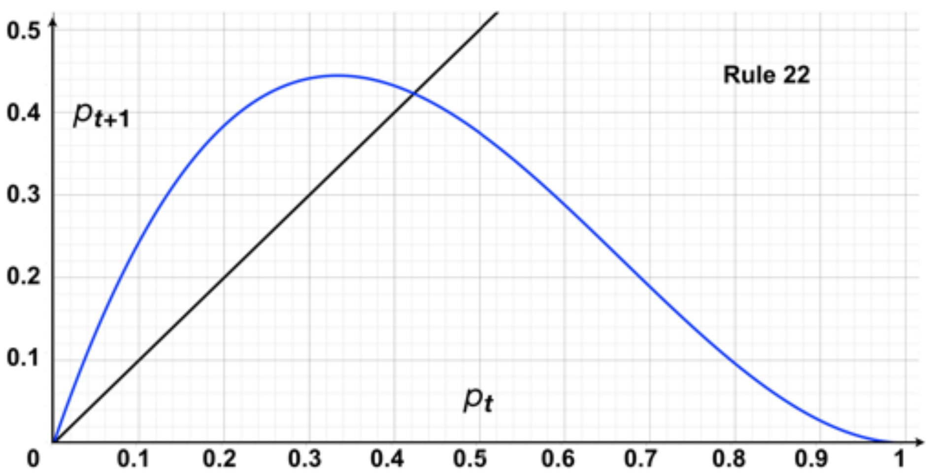
For one dimension, we adjust Eq. 3 to a full local rule and not only a semi–totalistic one. All states of the neighborhood must be considered, thus , , , and have the same representation as above. But now the product will be with the value of each neighborhood, whence, for a 1 CA the mean field polynomial
which gives
| (5) |
for ECA and where denotes the –th transition of in Eq. 1. Finally, the mean field polynomial for Rule 22
| (6) |
is deduced from (2).
In Rule 22 state ‘1’ appears with probability (which is close to the fixed stable point 0.37 of GoL). The mean field curve of Eq. 6 displayed in Fig. 2b shows a slope at the origin. Density is maximal at before reaching the stable fixed point when crossing the identity at It then crosses the inflection point with tangential slope and decreases until Based on the mean field curves classification, Rule 22 is a chaotic ECA (Fig. 3).

2.3 Mean field behavior of Rule 22
Various scenarios of evolution are displayed in Fig. 4:

- •
() From initial density reaching spontaneously the maximum before evolving rapidly towards the fixed point with density . Transition from to is not perceptible. () From initial density reaching spontaneously the fixed point.
- •
() From initial density evolving towards the fixed point after an early phase transition. () From initial density evolving towards the fixed point after a later phase transition delimited by a polygonal broken line11 1 Phase transitions and critical exponents for Rule 22 leading to non–trivial long–range effects were reported in [10, 11]. Asymptotic properties were described in [12]. . There exists an interval between two thresholds and such that any (pseudo–)random initial distribution with density converges almost surely towards fixed point .
- •
() From initial density evolving towards a dense pattern with observable ‘‘backbones’’22 2 Also observable in the “Exactly 1” ECA [13] Fig.1d. after crossing the phase transition polygon; two backbones arise from polygon vertices and their patterns are symmetric from either side. () From the same density and another initial distribution yielding a sparse pattern with backbones wherein no phase transition line does appear.
Outside interval sensitivity to initial conditions is high, with a positive Lyapunov exponent and a chaotic behavior. Depending on small perturbations from initial configuration, four other evolutions are also possible: (i) disordered sparse fractals (ii) convergence towards fixed point but after a long period (Fig. 5) (iii) initial configuration vanishing at first step (iv) rare events of periodic patterns (Fig. 6). That is, six types of evolution altogether. Their estimations of occurrence in interval are displayed in Tab. 1.
| Density | ERG | DSF | DBB | SBB | VAN | RPP |
|---|---|---|---|---|---|---|
| 100 | 0 | 0 | 0 | 0 | 0 | |
| 94 | 5 | 1 | 0 | 0 | 0 | |
| 93 | 1 | 3 | 1 | 1 | 1 | |
| 85 | 2 | 7 | 4 | 2 | 0 | |
| 47 | 4 | 13 | 24 | 12 | 0 | |
| 21 | 2 | 26 | 26 | 25 | 0 | |
| 7 | 0 | 18 | 21 | 54 | 0 | |
| 1 | 0 | 5 | 8 | 86 | 0 | |
| 0 | 0 | 0 | 0 | 100 | 0 |


Beyond the phase transition polygon in case of convergence towards fixed point , the evolution becomes ergodic, in the sense that the system has the same behavior either averaged over time or averaged over space [14]. The process is stationary and homogeneous at mesoscopic scale. In other words, their exists a smallest macro–cell of size where is the correlation length, as representative (or statistical) volume element such that density in the macro–cell is close to the mean density averaged within the whole system [15, 16]. Thus that is, the exact ratio of ‘1’ filling
It should be observed that a disordered sparse fractal pattern (DSF) may evolve towards ergodicity (ERG) as in Fig. 5 but sometimes after a long, unpredictable time. We denote as “DSF” such evolution remaining in this state at least within a time window of arbitrary length . In the same way, sparse backbone patterns (SBB) may evolve towards a dense backbone landscape (DBB).
A simple way to check (not to prove) whether unstable evolutions become eventually ergodic or to get a more global overview upon evolution is to skip some timesteps with skip time–lengths . This transformation yields a projective view upon the –landscape with angle Various skipped scenarios of evolution from initial critical density in a ring of 800 cells and within a time window of length are displayed in Fig. 7:

- •
() Phase transitions () DSF ERG with from disordered sparse fractal to ergodicity – up to 32000 generations, transition occurs after about 8000 timesteps () SBB DBB with from sparse to dense backbones – up to 31000 generations; transition occurs after about 4000 timesteps. Note that apparent discrepancies between densities in () and () before phase transition is no more than a side effect resulting from even or odd skip length parity.
- •
() Stratified landscapes SBB with () up to 64000 generations with observable backbones… and sub–backbones evolving like a Cantor dust () up to generations with perpetual phase transitions.
Failing to prove the existence or not of ergodic evolution, this skipping approach nevertheless emphasizes several chaotic behavior with long–range correlations. As well as in statistical physics, renormalization methods [15] overcome the weakness of mean field approximations that may fail or, at least, produce insufficient information. Mean field theory is a rough approximation which assumes independence between neighboring sites. On the contrary, other deterministic approaches like de Bruijn diagrams assume dependence. They will be discussed thereafter.
3 Attractors
3.1 Basins of attraction


Basins of attraction have been studied by Andy Wuensche in the framework of ECA and random Boolean networks [17, 18, 19]. A string of cell–states is a configuration . An evolution is represented by a sequence of configurations , such that , and the global transition can be represented as . A number of all global states of is determined by the length of a string (where is the length and the number of symbols). The structure of an attractor (Fig. 8) is given in three parts. Leaves represent Garden of Eden, i.e. unreachable in the evolution but only as initial global states (these states have no ancestors). Branches are configurations that have at least one ancestor and just one successor. Height of branches determines a number of generations to reach the attractor. An attractor is the final state of a string of length . Numbers labelling vertices represent the decimal values of the strings.
Wuensche [17] proposed that Wolfram’s classes can be represented as a basin classification. In this classification complex behavior is characterized by moderate transients, moderate–length periodic attractors, moderate in–degree and small density of leaves. This way, Fig. 9 displays a type of non–trivial behavior later of thousands of generations starting with a concatenation of one of these strings calculated by one attractor of length 20:
00000001000100000000 00000011101110000000
00000100000001000000 00001110000011100000
00010001000100010000 00111011101110111000
01000000000000000100 11100000000000001110
00010000000000010000 00111000000000111000
01000100000001000100 11101110000011101110.
Particularly, the average density for this evolution space is 4/15. This density lives exactly between the density of the rule itself (Eq. 2) and the stable fixed point in mean field theory (Eq. 6 and Fig. 2b). We will note that this value is not reachable from the statistical analysis done for ECA Rule 22. Also, it is the average where we report non–trivial behavior in ECA Rule 22. Of course, when an evolution is evolving to this value and later switches to the density of the stable fixed point hence the phase transition is irreversible (see Fig. 3).
By calculating large attractors, we can discover landscapes of complexity in basins featured with non–symmetric, high and dense ramifications: these kind of ramifications are indicators of ‘unpredictable’ behavior on most large configurations. No rarely chaotic rules tend to have symmetric basins. Basins of attraction can be connected into a meta–network, called the ‘jump-graph’ [18]. Jump–graphs determine the next level of CA complexity by showing a probability to jump from one attractor to another attractor given a mutation on the same domain of strings [20].

Let us consider a one–bit value mutation [18]. A configuration expressed as a string , such than it can jump into other configuration expressed as a string . Hence can mutate to one , where each configuration belongs at the same field of attractors . Also, the mutation represents a loop in the same basin if . Figure 10 shows a jump–graph from the basins of attraction of length 20 (Fig. 8). This way, a chaotic system presents a high density of connectivity with all the attractors in the jump–graph.
3.2 Longest paths and representative cycles
In this section we will use the term state as an alias for global state , configuration, or 1 string. CA() denotes an ECA Rule 22 with cells and cyclic boundary. The aim of this section is to study
- •
What is the length of the longest path until the zero-state is reached, and how does a related initial Garden of Eden state look like?
- •
How many cycles exist, how long are they, and what is a representative state for each cycle? Cycles that belong to the same class (cycles’ states are equivalent under shift and mirroring) shall be listed only once as representative cycle, the kind of cycles we are interested in here.
- •
Are there similar states (cyclically shifted) that appear periodically within a cycle?
- •
What is the length of the longest path until a certain cycle is reached, and how does a related initial state look like?
The following terms and functions are used here:
- •
path(A, C) is a sequence of states (from state to state ).
- •
length(path) gives the number of states of a path or cycle.
- •
prefix(C) is a path(, ) where is direct predecessor of .
- •
maxprefix(C) is a prefix() of maximum length.
- •
= length(maxprefix(0)) where (0) is the zero-state (00…0), the longest prefix(0).
- •
cycle denotes a periodic attractor, a cyclic path.
- •
k-cycle is a cycle of length .
- •
gives the length of a cycle.
- •
similar(S) is a state that can be derived from state by cyclic shift and optional mirroring.
- •
is called intra-cycle-period.
- •
In some cycles similar states appear again after time-steps.
- •
k/e-cycle is a -cycle where (-cycle). We may call -cycles strong if , and weak if .
- •
cycle-prefix is a prefix() where belongs to a cycle.
- •
gives the length of the longest cycle-prefix.
First method and results. The CA(), , were simulated for all possible initial states and then analyzed by special programs and manual inspection. In order to avoid unnecessary simulations, similar initial states were excluded. Similar states are states which are equivalent under cyclic shift and mirroring. For instance the number of different cases to be simulated for is only 7685, which is significantly lower than . It should be noted that the cycles for up to 34 were already computed by McIntosh [35].
| : length | normalized | |
|---|---|---|
| max prefix(0) | initial state | |
| 3 | 2 | 001 |
| 4 | 2 | 0001 |
| 5 | 6 | 01011 |
| 6 | 5 | 010111 |
| 7 | 6 | 0001111 |
| 8 | 8 | 00101011 |
| 9 | 2 | 000100101 |
| 10 | 7 | 0010111101 |
| 11 | 6 | 00101010101 |
| 12 | 23 | 001001100111 |
| 13 | 20 | 0001001100111 |
| 14 | 24 | 00010101100111 |
| 15 | 32 | 001001010100111 |
| 16 | 41 | 0000000101010011 |
| 17 | 53 | 00101010101110011 |
| 18 | 8 | 000001011000010011 |
| 19 | 17 | 0000101010111010101 |
| 20 | 18 | 00001000101010111101 |
| representative | repetition | initial state | ||||
| cycle state | within | of longest | ||||
| (normalised) | cycle | cycle-prefix | ||||
| 3, 5, 6 | no cycle | |||||
| 4 | 2 | (0011)* | 1 | =shl2() | 0 | no prefix |
| 7 | 7 | (0001011)* | 1 | =shl4() | 0 | no prefix |
| 2 | (0011)* | 1 | =shl2() | 0 | no prefix | |
| 8 | 4 | 00000101 | 2 | =shl4() | 2 | 00100111 |
| 6 | 00000011 | 3 | =shl4() | 2 | 00101101 | |
| 9 | 4 | 000000101 | 9 | 000100111 | ||
| 4 | 0000001001 | 2 | =shl5() | 7 | 0011010101 | |
| 10 | 4 | 0000000101 | 5 | 0010110011 | ||
| 6 | 0000010011 | 3 | =shl3m() | 1 | 0000010011 | |
| 4 | 00000001001 | 7 | 00000100111 | |||
| 11 | 5 | 00000001111 | 7 | 00101010011 | ||
| 11 | 00001001111 | 1 | =shl7() | 9 | 00010110011 | |
| 12 | 2 | (0011)* | 1 | =shl2() | 0 | no prefix |
| 4 | 000000010001 | 2 | =shl6() | 6 | 000100110011 | |
| 5 | 000000001111 | 9 | 001010101101 | |||
| 13 | 5 | 0000000001111 | 13 | 0000101001101 | ||
| 14 | 7 | (0001011)* | 1 | =shl3() | 0 | no prefix |
| 12 | 00000010001111 | 6 | =shl9m() | 4 | 00000101010011 | |
| 15 | 20 | 000000010000011 | 4 | =shl4() | 20 | 001010100101111 |
| 2 | (0011)* | 1 | =shl2() | 0 | no prefix | |
| 16 | 4 | (00000101)* | 2 | =shl4() | 2 | (00100111)* |
| 6 | (00000011)* | 3 | =shl4() | 2 | (00101101)* | |
| 7 | 000000000000011 | 11 | 0000000010010101 | |||
| 12 | 000000000000101 | 6 | =shl8() | 29 | 0000001001010111 | |
| 12 | 000000000100001 | 10 | 0010101010101011 | |||
| 4 | 000010100000101 | 2 | 00100101100100111 | |||
| 17 | 12 | 000000000000101 | 21 | 00101010101101011 | ||
| 26 | 000000000010011 | 13 | =shl15m() | 26 | 00101010010110011 | |
| 4 | 000100100000101 | 2 | =shl4() | 2 | 00101010100101101 | |
| 4 | (000000101)* | 45 | 00111001010101111 | |||
| 18 | 4 | 000010100000101 | 5 | 00101010011001111 | ||
| 12 | 000000000001001 | 6 | =shl9() | 35 | 00000001000011101 | |
| 12 | 000000000000101 | 55 | 00010010100110011 | |||
| 18 | 000001101001011 | 9 | =shl9() | 7 | 01111001100110011 | |
| 4 | 000100100000101 | 21 | 00001011100010111 | |||
| 4 | 000101000000101 | 6 | 10100101010101011 | |||
| 19 | 4 | 001001000000101 | 1 | 00110111000110111 | ||
| 12 | 000000000001001 | 78 | 00001100010010111 | |||
| 28 | 000001000011101 | 14 | =shl4m() | 9 | 01001100110011101 | |
| 2 | (0011)* | 1 | =shl2() | 0 | no prefix | |
| 4 | (0000001001)* | 2 | =shl5() | 44 | 00101100011010011 | |
| 4 | 001000100000101 | 2 | =shl4() | 5 | 00110110011001000 | |
| 4 | (0000000101)* | 12 | 11010001110101111 | |||
| 20 | 4 | 001001000001001 | 62 | 01111001010101111 | ||
| 4 | 001001000000101 | 10 | 00010000100001111 | |||
| 6 | 100110000101111 | 3 | =shl7m() | 1 | 01011010100101111 | |
| 6 | (0000010011)* | 3 | =shl7m() | 8 | 00001010100010111 | |
| 8 | 000000001000001 | 4 | =shl10() | 42 | 00000010001110101 | |
| 12 | 000000000010001 | 6 | =shl10() | 24 | 00100101100100011 | |
| 24 | 000000000100001 | 98 | 01010101110101101 |
Table 2 shows (the length of the maxprefix(0)), and the related normalized initial state. A normalized state is a representative of all states which are equivalent under cyclic shift and mirroring. It is found by selecting the state with the smallest binary number among all equivalents. E.g. normalize(100011) = 000111, and normalize(110110100) = 001011011 (by mirror and shift). The values are much smaller than , and not monotonically increasing with .
Table 3 shows the results obtained by analyzing all the simulations. The operator means shift to the left by positions, and means that first the mirror operator is applied before shifting.
We find always the trivial cycle of length 1. For even there always exists the fixed point (01)* (01)*, a lonely 1–cycle with no prefix. We will not further mention or pay special attention to these basic 1–cycles.
For , and multiples of 4, we get the 2/1–cycle (0011)* (1100)*. The two strings are similar under shift of two positions, so the inherent pattern is the same.
For , and multiples of 7, we get a 7–cycle. In order to characterize this cycle, one representative is chosen, it is the one with the smallest normalized value, i.e. (0001011)*.
For , we get three cycles with length .
For , there exists a 6/3–cycle. After every 3 time-steps, the same string appears in mirrored form and shifted 3 positions to the left.
For , the cycles of CA(4) form a subset (to be included if not detected) which is the 2/1-cycle (0011 0011 0011) (110 1100 1100).
For , the cycles of CA(7) form a subset which is shown as 7/1–cycle.
Fig. 8 shows all possible cycles where many of them are similar (equivalent under shift and mirroring). From that figure we may anticipate a very complex attractor structure, but we should realize that the number of representative cycles in CA(20) is only 11.
In general, because of the cyclic boundary, if is a factor of , then the CA() cycles are a subset of the CA() cycles. For example, the cycles of CA() form a subset of the CA() cycles. However there is a difference: the strings of CA() are cyclic repetitions of the CA() strings, and the original intra-cycle period may not appear in CA().
Second method and results. For larger , the first method cannot further be applied due to extensive computational costs. Therefore, now only a relatively small random subset of all possible initial states is used in order to find a subset of all cycles and paths which are not necessarily the longest ones.
10,0000 random initial states were generated for . For 5,000 of the states the probability 0.125 was used for each cell to generate a cell state 1. For the other 5,000 of the initial states, at first a probability between 0 and 1 (in steps of 1/1000) was randomly selected. Then was used for each cell to generate a cell state 1, otherwise 0. This technique of randomizing gave better results in experiments for Rule 22 compared to the usage of a fixed probability of 0.5. CAs were simulated and cycles and path lengths were computed and processed in a semi-automatic mode. In addition, a genetic algorithm was used to find near-optimal -values. The results are presented in Table 4. Note that because of the statistical approach, the listed cycles are not complete and the true maximum path lengths could be longer, e.g. for CA(60) all cycles already found for the factors CA(4, 5, 10, 12, 15, 20, 30) have to be included.
We can summarize that for , the longest paths are much smaller than (which is achievable with other ECA rules [21]). Further work remains to find a general formula or at least boundaries for the longest paths and the cycle distribution, depending on a number of cells.
| length of cycles | longest path | longest | |
| detected | ending in a cycle | prefix(0) | |
| 25 | 152 | ||
| 30 | 419 | ||
| 35 | 179 | ||
| 40 | 303 | ||
| 45 | 540 | ||
| 50 | 750 | ||
| 55 | 13904 | ||
| 60 | 35579 | ||
4 De Bruijn diagrams
De Bruijn diagrams [22] were originally proposed in shift–register theory [23]. For a 1 CA the de Bruijn diagram is defined as a directed graph with vertices and edges. Vertices are labelled with the elements of symbols of length . An edge is directed from vertex to vertex , if and only if, the final symbols of are the same as the initial ones in forming a neighborhood of states represented by . In this case, the edge connecting to is labelled with (the value of the neighborhood defined by the local function) [24], as shown in Fig. 11 for ECA(2,1) and for Rule 22 in Figs. 12–13.
4.1 Basic de Bruijn diagram
The connection matrix corresponding to the de Bruijn diagram [25] is as follows:
| (7) |


wherein module represents the number of vertices and takes on values in Hence for ECA(2,1)
| (8) |
and vertices are labelled by fractions of the overlapping of neighborhoods originated by 00, 01, 10 and 11, and the overlaps of the full neighborhood determine each connection:
They are the edges of the generic de Bruijn diagram in Fig. 11. The de Bruijn diagram has four vertices which can be renamed as corresponding to four partial neighborhoods of two cells , and eight edges representing neighborhoods of size . De Bruijn diagram for Rule 22 is derived from the generic one (Fig. 11) and it is calculated in Fig. 12, where the edges are labelled by the next state.

Paths in the de Bruijn diagram may represent chains, configurations or classes of configurations in the evolution space. Vertices are sequences of symbols in the set of states and the strings are sequences of vertices in the diagram. The edges represent overlapping of the sequences. Different intersection degrees evoke different de Bruijn diagrams (Fig. 13). Thus, the connection takes place between an initial symbol, the overlapping symbols and a terminal one. For practical reasons we can use colors, thus the color of an edge represents the next state to which each neighborhood, as shown in Fig. 11, evolves.


4.2 Extended de Bruijn diagram
An extended de Bruijn diagram [25, 6] takes into account wide overlapping of neighborhoods. We represent by indexes , where , and , and , and so up to with ; consequently basic de Bruijn diagram is obtained when . The regular expressions derived from the de Bruijn diagram for Rule 22 (Tab. 5) can be linked to space–time dynamics phenomena exhibited by the rules. These includes symmetric complex behavior, chaos, stable periodic behavior. Figure 14 shows in detail every periodic pattern yielded from extended de Bruijn diagrams. To read the diagram we use notation , where is a displacement (left or right) and is a number of generations. Thus the pattern in position (upper center) displays a periodic pattern without both displacement and period, the expression reproducing this pattern is (de Bruijn subdiagram in Fig. 14 and Eq. 2 in Table 5).


In this way, a lot of non-trivial patterns can be extracted. Let us consider few examples.
- •
. The graph is characterized by two cycles, the small cycle yielding simple still life patterns and the large cycle represents configurations emitting traveling localizations, ro particles. These configurations can not evolve naturally, i.e. from an initial random conditions, because they are destroyed when a certain limit of their size is reached (Fig. 15). They configurations are expressed for the following cycle–ways:
The regular expression to reproduce the same pattern is calculated as Eq. 8 in Table 5.
- •
. The graph has several paths between different cycles. Some of these cycles calculate trivial patterns. Other cycles represent configurations developed from a ‘fusion’ of two periodic regions competing for the space (Fig. 16). Other fused configurations can be found in coordinates (6,9), , , , , and .
- •
. Here we observe composed triangular polygons. The polygons sustain in a periodic mobile background. The background features small particles crossing the space (Fig. 17). This complex behavior emerges with probability between 1/7 and 3/7. This complex behavior was discovered with the help of expressions derived from the basins of attraction (see Fig. 9). One more example of interaction of large triangular domains evolving in the periodic background is shown in Fig. 18.
- •
. The periodic background is stationary. Several types of triangular domains and several families of small tiles emerge (Fig. 19). Other coordinates leading to similar configurations are , , , and .
During the analysis of configurations derived with the de Bruijn diagrams and basin of attractors we have referred to some specific regular expressions. Regular expressions can be calculated recursively by following paths on a graph with [26]:
| (9) |
where is the initial state and the final state. Base case when is the direct path to every node. This way, by using the basic de Bruijn diagram in Fig. 12, we have calculated the whole set of regular expressions, summarized in Table 5. The first column shows an equation number, the second column the regular expression, and the third column the kind of behavior that emerges when we codify configurations by these regular expressions. This way, we could evaluate these equations and explore an unlimited number of configurations.
| Eq | expression | evolution |
|---|---|---|
| 1 | stable state | |
| 2 | stable periodic | |
| 3 | stable state | |
| 4 | still life & symmetric complex behavior | |
| 5 | stable periodic & symmetric complex behavior | |
| 6 | stable state | |
| 7 | stable periodic, chaos & big gaps | |
| 8 | chaos, complex behavior | |
| 9 | complex behavior | |
| 10 | chaos, stable periodic, chaos & big gaps | |
| 11 | chaos, still life & symmetric complex behavior | |
| 12 | stable state, stable periodic, chaos & big gaps | |
| 13 | chaos, stable periodic, chaos & big gaps | |
| 14 | – | |
| 15 | – |
5 Garden of Eden
The question “does a complex CA contains a universal constructor?” is a classic problem appearing in the CA literature since von Neumann works [27]. A configuration of a universal constructor in the Game of Life CA is proposed by Goucher in 2010 [28]. In this context, our aim is to know if ECA Rule 22 is able to construct any string. Previously this problem was studied by McIntosh [6] who found that Rule 22 has a global injective relation and therefore configurations without ancestors exist.
We use a subset diagram to calculate Garden of Eden configurations [6], i.e., the configurations without ancestors [29]. A subset diagram has vertices with states and neighbors. If all the configurations of the certain length have ancestors then all the configurations with extensions both to the left and to the right with the same equivalence must have ancestors. But if this is not the case, then the vertices represent Garden of Eden configurations.
We can define the subset diagram as the power set of . Such that each subset (where is a power set) and one symbol :
| (10) |
Vertices of the subset diagram are formed by the combination of each subset formed from the states of the de Bruijn diagram. Symbolic de Bruijn matrices or are characterized by states and number of states in the partial neighborhood. Thus, for Rule 22 we can obtain symbolic matrices, derived from the de Bruijn sub–diagrams shown in Fig. 13. For any ECA we have four sequences of states in the Bruijn diagram enumerated as 0, 1, 2 and 3 (see Fig. 11).
Union between subsets is represented by the state in which each sequence evolves and is assigned to the states (subsets that form it) as governed by Eq. 10. Relations between subsets for Rule 22 are constructed in Table 6. Figure 20 shows the full scalar subset diagram. Each class of edges defines a function on or . The subset diagram describes the union that by itself is not functional [25].

We must distinguish four types of subsets, where it is possible to make a transition between its four unit classes. Also, we should observe that a residual of the de Bruijn diagram can be found in the subset diagram. This is because a unit class is precisely defined by the nodes of the original diagram. At first instance, we can see some relations are more frequent than others. Also there are nodes without inputs, or nodes with most connections including loops. Most important are cycles of different lengths. They are used to infer words, or sequences, that a CA could recognize. Thus, the subset diagram can be used as a general machine to recognize the universe of words in which a CA could evolve.
| label | 0 | 1 | |
|---|---|---|---|
| 0 | 0 | 0 | |
| {0} | 1 | 1 | 2 |
| {1} | 2 | 0 | 12 |
| {2} | 4 | 1 | 2 |
| {3} | 8 | 8 | 4 |
| {0,1} | 3 | 1 | 14 |
| {0,2} | 5 | 1 | 2 |
| {0,3} | 9 | 9 | 6 |
| {1,2} | 6 | 1 | 14 |
| {1,3} | 10 | 8 | 12 |
| {2,3} | 12 | 9 | 6 |
| {0,1,2} | 7 | 1 | 14 |
| {0,1,3} | 11 | 9 | 6 |
| {0,2,3} | 13 | 9 | 6 |
| {1,2,3} | 14 | 9 | 14 |
| {0,1,2,3} | 15 | 9 | 14 |
By analyzing the full diagram we can derive a small subset diagram which is deduced from the original diagram (de Bruijn diagram). This diagram includes only vertexes with cycles, the universal and empty set and the subset with one element, yielding a new diagram that will be more practical for us. The reduction gives yet a more small diagram to read quickly strings belonging to Garden of Eden configurations. The reduction is also useful to calculate the degree of Welch indices for reversible CAs [30]. The expressions that determine Garden of Eden configurations in ECA Rule 22 are listed below:
- •
10110
- •
01111*01101*
- •
11*(011111)*1*0110
6 Fractals
6.1 Iterated functions in Rule 22
A fractal is constructed recursively from a self–replication of a pattern [31]. Chaotic systems often bear properties of fractals.


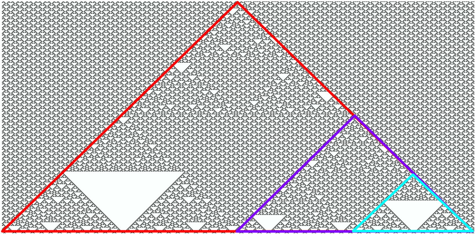


ECA Rule 22 produces a fractal pattern, known as Sierpiński triangle, starting from a single cell in state 1 (Fig. 1). Figure 21 shows a triangle constructed with three small tiles derived in Rule 22, this triangle grows in power of two with respect the number of cells. The main triangle (Fig. 21a) has three replicas in the next iteration (Fig. 21b), and following iteration produces nine base replicas (Fig. 21c). The fractal dimension can be calculated given the number of replicates and the scaling factor [32]. The fractal dimension of the patterns generated by Rule 22 is the following:
| (11) |
Also ECA Rule 22 displays non trivial behavior via fractals where they emerge in different stages during the evolution. These fractals are combined with other fractals constructed from Rule 22 over thousands of generations.
Using regular expressions we found two different periodic backgrounds emerging in ECA Rule 22, as discussed in Sections 5, 6 and 7. Let us illustrate two fractals growing in intervals of other fractals with different composition of tiles. Figure 22a shows the initial state of fractals growing in a periodic background without displacement conserving the same fractal dimension. Figure 22b shows the same iterated function over thousands of generations. The same behavior is tested on a periodic background with displacement in Figs. 23ab. Composed fractals emerging in periodic backgrounds with or without displacement are disjoint.
6.2 Rule 18, mutations, gaskets and seashells
| Rule | 111 | 110 | 101 | 100 | 011 | 010 | 001 | 000 | Mutation |
| 18 | 0 | 0 | 0 | 1 | 0 | 0 | 1 | 0 | |
| 22 | 0 | 0 | 0 | 1 | 0 | 1 | 1 | 0 | |
| 26 | 0 | 0 | 0 | 1 | 1 | 0 | 1 | 0 | |
| 30 | 0 | 0 | 0 | 1 | 1 | 1 | 1 | 0 | |
| 50 | 0 | 0 | 1 | 1 | 0 | 0 | 1 | 0 | |
| 54 | 0 | 0 | 1 | 1 | 0 | 1 | 1 | 0 | |
| 58 | 0 | 0 | 1 | 1 | 1 | 0 | 1 | 0 | |
| 62 | 0 | 0 | 1 | 1 | 1 | 1 | 1 | 0 | |
| 82 | 0 | 1 | 0 | 1 | 0 | 0 | 1 | 0 | |
| 86 | 0 | 1 | 0 | 1 | 0 | 1 | 1 | 0 | |
| 90 | 0 | 1 | 0 | 1 | 1 | 0 | 1 | 0 | |
| 94 | 0 | 1 | 0 | 1 | 1 | 1 | 1 | 0 | |
| 114 | 0 | 1 | 1 | 1 | 0 | 0 | 1 | 0 | |
| 118 | 0 | 1 | 1 | 1 | 0 | 1 | 1 | 0 | |
| 122 | 0 | 1 | 1 | 1 | 1 | 0 | 1 | 0 | |
| 126 | 0 | 1 | 1 | 1 | 1 | 1 | 1 | 0 |
Rule 18 and Rule 22 are complex rules widely reported in ECA literature [33, 34, 35, 11, 13]. Let us redefine them as follows: a cell takes state ‘1’ if exactly one
- •
(R18): of its neighbors is in state ‘1’:
- •
(R22): in its neighborhood is in state ‘1’:
and consider the subset of the 256 ECA
| (12) |
that defines the sixteen rules displayed in Tab. 7. Referring to the genotype paradigm in [36] with a rule defined by the sequence a rule mutates into Rule through bit (or “gene”) , or with exactly a 1–bit change, that yields the mutation (or inheritance) tree in Fig. 24.
This tree contains a set of rules with complex behavior inherited from Rule 18 and where Sierpiński patterns often appear. Rules 18, 22, 122, 126 reveal a similar behavior towards ergodic regime and unstable areas, as well as Rule 90 but that displays a multilayered pattern, whereas Rule 30 and, by reflection, Rule 86 exhibit small striped patterns near the polygonal border. Rule 26 and, by reflection, Rule 82 exhibit large striped patterns at equilibrium, that may evolve towards sparse backbones at low or high densities, or periodic patterns similar to those in Fig. 6. Rule 94 displays a Sierpiński gasket, but evanescent and quickly entering a uniform polygon with vertical stripes. Finally it should be emphasized that Rules 50, 54, 58 and by reflection 114, 62 and by reflection 118, display patterns somewhat far from the sieve but nevertheless all of them enter the phase transition polygon33 3 Rules 30, 54, 90, 126 are examined elsewhere [37, 38, 39, 40]. .


This tree does not contain the subset of rules associated either by conjugation or by conjugation-reflection. Beginning from Rule 129 –conjugate with Rule 126– this subset would display a large collection of Sierpiński–like patterns but this time in white on a black background.
Even in the synchronous “1nCA” [41] with a minimal neighborhood of two cells –the cell itself and the either left or right adjacent cell alternating at either odd or even timesteps– Sierpiński patterns appears in Rules 6 and 9, namely for the only symmetric rules with an equal number of black and white cells, and for the only rules fulfilling the maximal “sensitivity parameter”.


Six rules (18, 22, 30, 90, 122, 126) evolving in their ergodic regime are displayed in Fig. 25. All patterns have the Hausdorff dimension of Eq. 11. They only differ from their average density of their mesoscopic minimal macrocell
Referring again to the mean field curves in Sect. 2 now displayed for Rule 18 and Rule 22 in Fig. 26 we observe that Rule 18 curve reaches its stable fixed point when crossing the identity at whereas for Rule 22 the fixed point is got at whence the discrepancies between densities in ergodic regime, observable in Fig. 25. Moreover, Rule 18 curve shows a slope whereas Rule 22 shows a slope at the origin. That comes from the fact that these rules induce from a single source their following evolution:
- •
(R18):
- •
(R22):
and that their density ratio at timesteps () remains .
The Sierpiński gasket [42] appears in a wide variety of situations [43]. The binomial coefficients can be arranged to form Pascal’s triangle and Pascal’s triangle turns into Sierpiński gasket with coefficients modulo two. It may turn into something like a natural tree by some diffeomorphism. This tree is embeddable into the 2 diffusion graphs embedded into the triangulate lattice [44, 45]: its vertex dust forms the Sierpiński gasket patterns. Sierpiński gasket is often known as a Banach fixed point from some contractive affine transformation into three elements.
But the most fascinating is the formation of patterns from random initial distributions of pigmentations on certain varieties of seashells [33, 46]. This phenomenon can be explained from the Gierer–Meinhardt reaction-diffusion model of the activator–inhibitor type, arising in various situations of pattern formation in morphogenesis [47, 48].
7 Discussion
7.1 Chaos or determinism?
Despite the fact that Rule 22 is based on simple and determined interactions, the behavior generated by such system is visibly complex and seems to be non–deterministic. To test the kind of the rule’s behavior tests chaos 0–1 [49] (classifier returning value near 1 if series is chaotic and near to 0 if deterministic) was used to determine whether behavior is chaotic/random or deterministic. It is applied directly to the time series data and does not require phase space reconstruction. These two kinds of behavior are significantly different. Physically, randomness has a stochastic nature, while deterministic chaos is generated by even simple system that does not contain any source of randomness, as commonly understood by public. If executed on a PC, then algorithms simulating such behavior generate only pseudo-random/chaotic behavior and series generated in such a way, are essential deterministic and periodic but with very long period. The period is usually long enough to simulate randomness/chaos.
The term chaos covers a rather broad class of phenomena whose behavior may seem erratic, chaotic at first glance. Till now chaos was observed in many systems (including evolutionary ones) and, in the last few years, it has been also used to replace pseudo-random number generators (PRGNs) in evolutionary algorithms (EAs). Let us mention for example research papers like [50] (a comprehensive overview of mutual intersection between EAs and chaos is discussed in this paper), one of the first use of chaos inside EAs [51], [52, 53] discussing the using of deterministic chaos inside particle swarm algorithm instead of PRGNs, [54, 55] investigating relations between chaos and randomness or the latest one [56], and [57, 58, 59], using chaos with EAs in applications, amongst others.
Another research joining deterministic chaos and pseudorandom number generator has been done for example in [54]. The possibility of generation of random or pseudorandom numbers by use of the ultra weak multidimensional coupling of 1-dimensional dynamical systems is discussed there. Another paper [60] deeply investigates a logistic map as a possible pseudo-random number generator and it is compared with contemporary pseudo-random number generators. A comparison of logistic map results is made with conventional methods of generating pseudo-random numbers. The approach is used to determine the number, delay, and period of the orbits of the logistic map at varying degrees of precision (3 to 23 bits). Logistic map, we are using here, was also used in [61] like chaos-based true random number generator embedded in reconfigurable switched-capacitor hardware. Another paper [62] proposed an algorithm of generating a pseudorandom number generator, which is called (couple map lattice based on discrete chaotic iteration) and combine the couple map lattice and chaotic iteration. Authors also tested this algorithm in NIST 800-22 statistical test suits and is used in image encryption.
In [63] authors exploit interesting properties of chaotic systems to design a random bit generator, called CCCBG, in which two chaotic systems are cross-coupled with each other. For evaluation of the bit streams generated by the CCCBG, the four basic tests are performed: monobit test, serial test, auto-correlation, Poker test. Also the most stringent tests of randomness: the NIST suite tests have been used.
A new binary stream–cipher algorithm based on dual one-dimensional chaotic maps is proposed in [55] with statistic properties showing that the sequence is of high randomness. Similar studies are also done in [51, 64, 65, 66]. For a long time various PRNGs were used inside evolutionary algorithms. During last few years deterministic chaos systems (DCHS) are used instead of PRNGs. As was demonstrated in [52, 53], very often the performance of EAs using DCHS is better or fully comparable with EAs using PRNGs. See for example [52].
The chaos test 0–1 [49] has been already and successfully used on various tasks as for example on experimental data from a bipolar motor [67], behavior of the cutting process [68], real experimental time series of laser droplet generation process [69] and validated by applying to typical nonlinear dynamic systems, including fractional–order dynamic system [70] amongst others.
The same approach was used here. Test 0-1 was used on different series in order to verify and test the nature of Rule 22. Figure 27 visualizes results of our experiments. For evaluation 2000 Rule 22 behavior strings of length 2000 have been used. The same was repeated for the Mersenne twister random number generator [71] (MTPRNG) (Fig. 27), chaos generated by logistic equation (LE) (Fig. 27), and periodic series (PS): the sinus function generated from the randomly selected position (Fig. 27). As clearly visible, test 0-1 has clearly classified Rule 22, MTPRNG and LE as a non-deterministic series while series based on periodic pattern as deterministic. The random series were not distinguished from chaotic ones. This was probably caused by insufficient length (2000 is likely not enough) of series, however, this was not a matter of this experiment.
7.2 Memory leads to complexity
In this section, we show that ECA Rule 22 with memory is strongly chaotic [72].
Conventional CA are ahistoric (memoryless): i.e., the new state of a cell depends on the neighborhood configuration solely at the preceding time step of . Thus, CA with memory (CAM) can be considered as an extension of the standard framework of CA where every cell is allowed to remember some period of its previous evolution. A memory is based on the state and history of the system, thus we design a memory function , as follows: , such that determines the backwards degree of memory and each cell is a function of the series of states in cell up to time-step . To execute the evolution we apply the original rule as follows: .


In CAM, while the mapping remains unaltered, a historic memory of past iterations is retained by featuring each cell as a summary of its previous states; therefore cells canalize memory to the map . As an example, we can take the memory function as a majority memory: , where in case of a tie given by in , we shall take the last value . So represents the classic majority function for three variables on cells and defines a temporal ring before calculating the next global configuration . In case of a tie, it is allowed to break it in favor of zero if , or to one whether .
The representation of a ECAM is given as follows:
| (13) |
where represents the decimal notation of a particular ECA rule and the kind of memory given with a specific value of .
Note that memory is as simple as any CA, and that the global behavior produced by the local rule is rather unpredictable, it can lead to emergent properties and so can be classed as complex. Memory functions were developed and extensively studied by Alonso-Sanz in [73]. Memory in ECA have been studied, showing its potential to produce complex behavior from chaotic systems and beyond in [37, 72], and recently in [74] authors have included hybrid versions. Thus, we can conjecture that a memory function can produce complex behavior [72] as follows:
| (14) |
Eppstein [75] demonstrates that a CA class IV is a system where mobile self–localizations emerge. We can relate type of classes with memory functions in ECA Rule 22 as:
| (15) | ||||
| (16) | ||||
| (17) | ||||
| (18) |
7.3 Rareness and unpredictability
The state transition function can be re-written as Boolean formula with two xor operations: . The xor gate is the most rare, most hard to find in natural non-linear systems, Boolean gate. Let gates and discovered with occurrence frequencies and , we say a gate is easier to develop or evolve than a gate : if . The hierarchies of gates obtained using evolutionary techniques in liquid crystals [78], light–sensitive modification of Belousov–Zhabotinsky system [79], slime mould Physarum polycephalum [80] and protein molecules [81, 82]:
- •
Gates in liquid crystals: {or, nor} and not nand xor
- •
Gates in Belousov–Zhabotinsky medium: and nand xor
- •
Gates in cellular automata [83]: or nor and nand xor
- •
Gates in Physarum: and or nand nor xor xnor
- •
Gates in protein molecules verotoxin and actin:
and or and-not xor
The xor gate is hard to find and space-time dynamics of Rule 22 automata is hard to predict. A strong link computational difficulty of a problem and its randomness was established by Yao [84]. His famous lemma, rephrased by Impagliazzo and Wigderson [85], can be seen in the framework of predictability of Rule 22 ECA behavior:
Fix a non-uniform model of computation (with certain closure properties) and a Boolean function . Assume that any algorithm in the model of a certain complexity has a significant probability of failure when predicting on a randomly chosen instance . Then any algorithm (of a slightly smaller complexity) that tries to guess the xor of random instances won’t do significantly better than a random coin toss.
Potential associations between dynamics in Rule 22 ECA and a role of xor functions in communication complexity [86, 87] could be explored in future.
References
- [1] S. Wolfram, Statistical mechanics of cellular automata, Rev. Mod. Phys. 55(3) (1983) 601–644.
- [2] S. Wolfram, Cellular Automata and Complexity (1994) Addison-Wesley Publishing Company.
- [3] S. Wolfram, Twenty Problems in the Theory of Cellular Automata, Physica Scripta 9 (1985) 170–183.
- [4] M. Redeker, A. Adamatzky, G.J. Martínez, Expressiveness of Elementary Cellular Automata, International Journal of Modern Physics C 24(3) (2013) 1350010–14.
- [5] J.G. Zabolitzky, Critical Properties of Rule 22 Elementary Cellular Automata, Journal of Statistical Physics 50(5-6) (1988) 1255–1262.
- [6] H.V. McIntosh, One Dimensional Cellular Automata, Luniver Press, UK (2009)
- [7] W. Jin, F. Chen, C. Yang, Topological Chaos of Cellular Automata Rules, Proceedings of International Workshop on Chaos–Fractals Theories and Applications (2009) 216–220.
- [8] H.A. Gutowitz, J.D. Victor, Local structure theory in more that one dimension, Complex Systems 1 (1987) 57–68.
- [9] H.V. McIntosh, Wolfram’s Class IV and a Good Life, Physica D 45 (1990) 105–121.
- [10] P. Grassberger, Long-Range Effects in an Elementary Cellular Automaton, J. Stat. Phys. 45 (1-2) (1986) 27–39.
- [11] S. Sinha, Phase Transitions in the Computational Complexity of “Elementary” Cellular Automata, Minai, A.A., Bar-Yam,Y. (eds.) Unifying Themes in Complex Systems. Springer (2011) 337–348.
- [12] H. Zenil, E. Villarreal-Zapata, Asymptotic Behaviour and Ratios of Complexity in Cellular Automata, International Journal of Bifurcation and Chaos 23(9) (2013) 1350159.
- [13] J. Gravner, D. Griffeath, The One-Dimensional Exactly 1 Cellular Automaton: Replication, Periodicity, and Chaos from Finite Seeds, J. Stat. Phys. 142(1) (2011) 168–200.
- [14] P. Halmos, Lectures on ergodic theory, Amer. Math. Soc. 142, 1956.
- [15] A. Lesne, Renormalization Methods, John Wiley and Sons, 1998.
- [16] D. Désérable, Embedding Kadanoff’s scaling picture into the triangular lattice, Acta Phys. Pol. B Proc. Suppl. 4(2) (2011) 249–265.
- [17] A. Wuensche, M. Lesser, The Global Dynamics of Cellular Automata, Addison-Wesley (1992)
- [18] A. Wuensche, Exploring Discrete Dynamics 2nd. Edition. Luniver Press, Bristol (2016)
- [19] H.V. McIntosh, Ancestors: Commentaries on The Global Dynamics of Cellular Automata, (1993) http://delta.cs.cinvestav.mx/~mcintosh/cellularautomata/Working_Papers_files/global.pdf
- [20] G.J. Martínez, A. Adamatzky, B. Chen, F. Chen, J.C. Seck-Tuoh-Mora, Simple networks on complex cellular automata: From de Bruijn diagrams to jump-graphs, In: Swarm Dynamics as a Complex Network, I. Zelinka, G. Chen (Ed.), Springer (2017) 241–264.
- [21] S. Adak, S. Mukherjee, S. Das, Do There Exist Non-linear Maximal Length Cellular Automata? A Study, G. Mauri, S. El Yacoubi, A. Dennunzio, K. Nishinari, L. Manzoni eds) Cellular Automata LNCS 11115 (2018) 289–297.
- [22] N.G. de Bruijn, A combinatorial problem, Proceedings of the Section of Sciences of the Koninklijke Nederlandse Akademie van Wetenschappen te Amsterdam 49(7) (1946) 758–764.
- [23] S.W. Golomb, Shift Register Sequences, Holden-Day, San Francisco (1967)
- [24] B.H. Voorhees, Computational analysis of one-dimensional cellular automata, World Scientific (1996)
- [25] H.V. McIntosh, Linear cellular automata via de Bruijn diagrams, http://delta.cs.cinvestav.mx/~mcintosh/cellularautomata/Papers_files/debruijn.pdf (1991)
- [26] J.E. Hopcroft, J.D. Ullman, Introduction to Automata Theory Languages, and Computation, Reading, Addison-Wesley (1979)
- [27] J. von Neumann, Theory of Self-reproducing Automata (edited and completed by A.W. Burks), University of Illinois Press, Urbana and London (1966)
- [28] A.P. Goucher, Universal Computation and Construction in GoL Cellular Automata, In: Game of Life Cellular Automata A. Adamatzky (Ed.) Springer (2010) 505–517.
- [29] S. Amoroso, G. Cooper, The Garden-of-Eden theorem for finite configurations, Proceedings of the American Mathematical Society 26(1) (1970) 158–164.
- [30] J.C. Seck-Tuoh-Mora, J. Medina-Marín, N. Hernández-Romero, G.J. Martínez, I. Barragán-Vite, Welch sets for random generation and representation of reversible one-dimensional cellular automata, Information Sciences 382–383 (2017) 81–95.
- [31] D. Eppstein, “Fractals”, http://www.ics.uci.edu/~eppstein/junkyard/fractal.html.
- [32] G. Chen, X. Dong, From Chaos to Order, World Scientific Series on Nonlinear Science, Series A, Vol. 24 (1998)
- [33] S. Wolfram, Cellular Automata, Los Alamos Science 9 (1983) 2–21.
- [34] S. Wolfram, Computation theory of cellular automata, Comm. Math. Phys. 96(1) (1984) 15–57.
- [35] H.V. McIntosh, Linear cellular automata, http://matematicas.reduaz.mx/~cellularautomata/cellularautomata/Papers_files/lcau.pdf (1990)
- [36] W. Li, N.H. Packard, The Structure of the Elementary Cellular Automata Rule Space, Complex Systems 4(3) (1990) 281–297.
- [37] G.J. Martínez, A. Adamatzky, R. Alonso–Sanz, J.C. Seck Tuoh Mora, Complex Dynamics Emerging in Rule 30 with Majority Memory, Complex Systems 18(3) (2009) 345–365.
- [38] G.J. Martínez, A. Adamatzky, H.V. McIntosh, Complete Characterization of Structure of Rule 54, Complex Systems 23(3) (2014) 259–293.
- [39] O. Martin, A.M. Odlyzko, S. Wolfram, Algebraic Properties of Cellular Automata, Comm. Math. Phys. 93(2) (1984) 219–258.
- [40] G.J. Martínez, A. Adamatzky, J.C. Seck Tuoh Mora, R. Alonso–Sanz, How to make dull cellular automata complex by adding memory: Rule 126 case study, Complexity 15(6) (2010) 34–49.
- [41] S. Bandini, A. Bonomi, G. Vizzari, An analysis of different types and effects of asynchronicity in cellular automata update schemes, Nat. Comp. 11(2) (2012) 277–287.
- [42] W. Sierpiński, O krzywej, której każdy punkt jest punktem rozgałȩzienia, Prace Mat.–Fiz. 27(1) (1916) 77–86.
- [43] M. Barnsley, Fractals everywhere, Acad. Press., San Diego, CA (1988)
- [44] D. Désérable, A family of Cayley graphs on the hexavalent grid, Discrete Applied Math. 93 (1999) 169–189.
- [45] D. Désérable, Systolic Dissemination in the Arrowhead Family, Cellular Automata, Wa̧s, J., Sirakoulis, G., Bandini, S. eds, LNCS 8751 (2014) 75–86.
- [46] H. Meinhardt, The Algorithmic Beauty of Seashells, The Virtual Laboratory, Springer (2009)
- [47] A. Gierer, H. Meinhardt, A theory of biological pattern formation, Kybernetik 12(1) (1972) 30–39
- [48] A. Turing, The Chemical Basis of Morphogenesis, Phil. Trans. Royal Soc. London 237(641) (1952) 37–72
- [49] G.A. Gottwald, I. Melbourne, On the implementation of the 0–1 test for chaos, SIAM Journal on Applied Dynamical Systems 8(1) (2009) 129–145
- [50] I. Zelinka, S. Celikovský, H. Richter, G. Chen, Evolutionary Algorithms and Chaotic Systems, (Eds), Studies in Computational Intelligence, Springer (2010)
- [51] R. Caponetto, L. Fortuna, S. Fazzino, M.G. Xibilia, Chaotic sequences to improve the performance of evolutionary algorithms, IEEE Trans. Evol. Comput. 7(3) (2003) 289–304.
- [52] M. Pluhacek, R. Senkerik, D. Davendra, Z. Oplatkova, On the Behavior and Performance of Chaos Driven PSO Algorithm with Inertia Weight, Computers & Mathematics with Applications 66(2) (2013) 122–134
- [53] M. Pluhacek, V. Budikova, R. Senkerik, Z. Oplatkova, I. Zelinka, On the Performance of Enhanced PSO algorithm with Lozi Chaotic Map – An Initial Study, In: Proceedings of 18th International Conference on Soft Computing – MENDEL 2012, (2012) 40–45
- [54] R. Lozi, Emergence of Randomness From Chaos, International Journal of Bifurcation and Chaos 22(2) World Scientific (2012) 1250021
- [55] X.-Y. Wang, L. Yang, Design of Pseudo-Random Bit Generator Based on Chaotic Maps, International Journal of Modern Physics 26(32) World Scientific (2012) 1250208
- [56] Y. Sun, L. Zhang, X. Gu, A hybrid co-evolutionary cultural algorithm based on particle swarm optimization for solving global optimization problems, Neurocomputing 98 (2012) 76–89
- [57] W-Ch. Hong, Y. Dong, W.Y. Zhang, L.Y. Chen; B.K. Panigrahi, Cyclic electric load forecasting by seasonal SVR with chaotic genetic algorithm, International Journal of Electrical Power and Energy Systems 44(1) (2013) 604–614
- [58] R. Senkerik, D. Davendra, I. Zelinka, Z. Oplatkova, M. Pluhacek, Optimization of the Batch Reactor by Means of Chaos Driven Differential Evolution, Soft Computing Models in Industrial and Environmental Applications, Springer, AISC 188 (2013) 93–102
- [59] D. Davendra, I. Zelinka, R. Senkerik, Chaos driven evolutionary algorithms for the task of PID control, Computers & Mathematics with Applications 60(4) (2010) 1088–1104
- [60] K.J. Persohn, R.J. Povinelli, Analyzing logistic map pseudorandom number generators for periodicity induced by finite precision floating-point representation, Chaos, Solitons and Fractals 45(3) (2012) 238–245
- [61] M. Drutarovsky, P. Galajda, A robust chaos-based true random number generator embedded in reconfigurable switched-capacitor hardware, 17th International Conference Radioelektronika (2007) 29–34
- [62] X.Y. Wang, X. Qin, A new pseudo-random number generator based on CML and chaotic iteration, Nonlinear Dynamics 70(2) (2012)1589–1592
- [63] N.K. Pareek, V. Patidar, and K.K. Sud, A Random Bit Generator Using Chaotic Maps, International Journal of Network Security 10!1) !2010) 32–38
- [64] M. Bucolo, R. Caponetto, L. Fortuna, M. Frasca, A. Rizzo, Does chaos work better than noise? IEEE Circuits and Systems Magazine 2(3) (2002) 4–19
- [65] HP. Hu, LF. Liu, N. Ding, Pseudorandom sequence generator based on the Chen chaotic system, Computer Physics Communications 184(3) (2013) 765–768
- [66] A. Pluchino, A. Rapisarda, C. Tsallis, Noise, synchrony, and correlations at the edge of chaos, Phys. Rev. E 87(2) (2013) 022910
- [67] I. Falconer, G.A. Gottwald, I.Melbourne, K. Wormnes, Application of the 0-1 test for chaos to experimental data, SIAM Journal on Applied Dynamical Systems 6(2) (2007) 395–402
- [68] G. Litak, A. Syta, M. Wiercigroch, Identification of chaos in a cutting process by the 0–1 test, Chaos, Solitons & Fractals 40(5) (2009) 2095-2101
- [69] B. Krese, E. Govekar, Nonlinear analysis of laser droplet generation by means of 0–1 test for chaos, Nonlinear Dynamics, 67(3) (2012) 2101–2109
- [70] S. Ke-Hui, L. Xuan, Z. Cong-Xu, The 0-1 test algorithm for chaos and its applications, Chinese Physics B, 19(11) (2010) 110510
- [71] M. Matsumoto, N. Takuji, Mersenne twister: a 623-dimensionally equidistributed uniform pseudo-random number generator, ACM Transactions on Modeling and Computer Simulation (TOMACS) 8(1) (1998) 3–30
- [72] G.J. Martínez, A. Adamatzky, A., R. Alonso-Sanz, Designing Complex Dynamics with Memory, Int. J. Bifurcation and Chaos 23(10) (2013) 1330035–131
- [73] R. Alonso-Sanz, Cellular Automata with Memory, Old City Publishing, Inc. (2009)
- [74] B. Chen, F. Chen, G.J. Martínez, Glider Collisions in Hybrid Cellular Automaton with Memory Rule (43,74), International Journal of Bifurcation and Chaos 27(6) (2017) 1750082
- [75] D. Eppstein, “Wolfram’s Classification of Cellular Automata”, https://www.ics.uci.edu/~eppstein/ca/wolfram.html.
- [76] G.J. Martínez, K. Morita, Conservative Computing in a One-dimensional Cellular Automaton with Memory, Journal of Cellular Automata 13(4) (2018) 325–346
- [77] G.J. Martínez, A. Adamatzky, K. Morita, Logical Gates via Gliders Collisions, In: Reversibility and Universality, A. Adamatzky (Ed.), Springer (2018) 199–220
- [78] S. Harding, J.F. Miller, Evolution in materio: Evolving logic gates in liquid crystal, International Journal of Unconventional Computing 3(4) (2007) 243–257
- [79] R. Toth, C. Stone, A. Adamatzky, B.d.L. Costello, L. Bull, Dynamic control and information processing in the Belousov–Zhabotinsky reaction using a coevolutionary algorithm, The Journal of Chemical Physics, 129(18) (2008) 184708.
- [80] S. Harding, J. Koutnik, J. Schmidhuber, A. Adamatzky, Discovering Boolean Gates in Slime Mould, In Inspired by Nature – Emergence, Complexity and Computation 28, S. Stepney, A. Adamatzky (Eds.) (2018) 323–337
- [81] A. Adamatzky, Computing in Verotoxin. ChemPhysChem 18(13), (2017) 1822–1830.
- [82] A. Adamatzky, Logical gates in actin monomer, Scientific reports 7(1) (2017) 11755
- [83] A. Adamatzky, L. Bull, Are complex systems hard to evolve? Complexity 14(6) (2009) 15–20.
- [84] A.C. Yao, Theory and application of trapdoor functions, SFCS’1982, 23rd Annual Symposium on Foundations of Computer Science, IEEE (1982) 80–91
- [85] R. Impagliazzo, A. Wigderson, P=BPP unless E has sub-exponential circuits: Derandomizing the XOR Lemma, Proceedings of the 29th Symposium on Theory of Computing STOC (1997).220-229
- [86] Z. Zhang, Y. Shi, Communication complexities of symmetric XOR functions, Quantum Information & Computation 9(3) (2009) 255–263
- [87] A. Montanaro, T. Osborne, On the communication complexity of XOR functions, Computational Complexity, arXiv:0909.3392 (2010) 1–18