Modeling multiple taxis: tumor invasion with phenotypic heterogeneity, haptotaxis, and unilateral interspecies repellence
Abstract
We provide a short review of existing models with multiple taxis performed by (at least) one species and consider a new mathematical model for tumor invasion featuring two mutually exclusive cell phenotypes (migrating and proliferating). The migrating cells perform nonlinear diffusion and two types of taxis in response to non-diffusing cues: away from proliferating cells and up the gradient of surrounding tissue. Transitions between the two cell subpopulations are influenced by subcellular (receptor binding) dynamics, thus conferring the setting a multiscale character.
We prove global existence of weak solutions to a simplified model version and perform numerical simulations for the full setting under several phenotype switching and motility scenarios. We also compare (via simulations) this model with the corresponding haptotaxis-chemotaxis one featuring indirect chemorepellent production and provide a discussion about possible model extensions and mathematical challenges.
1 Introduction
The growth, development, spread, and even survival of biological organisms and populations are tightly connected to their environment and its characteristics. A multitude of different biological and chemical species interact with each other and with their surroundings in order to perform the mentioned processes. Intra- and interpopulation reciprocities together with environmental heterogeneities have a decisive influence on the fate of individuals as well as populations. A prominent example is given by the motility and proliferation behavior of cells in response to biochemical and biophysical cues present in their extracellular space. Not only can these induce a pronounced migratory bias of the cells towards favorable signals or away from hostile ones (also known as taxis), but they can even determine their phenotype and interaction strategies. Moreover, cells are able to modify their environment according to their needs, a behavior which is obvious in higher species.
Since such complex processes and their mutual conditioning scenarios are difficult to assess experimentally, mathematical models can help understanding the underlying biological mechanisms, test hypotheses, make predictions, and even suggest new experiments and conjectures. During the last five decades the scientific community has witnessed an unprecedented development of mathematical descriptions of problems motivated by life sciences, and to a large extent by cell biology, triggered among others by Keller and Segel’s work on chemotaxis modeling [44].
Several fine reviews of chemotaxis models are available, see e.g. [2, 29, 34, 72], addressing aspects of well-posedness, long time behavior, and patterns. Without the pretension of exhaustiveness we provide a short review of existing models from the perspective of multiple taxis. By the latter we mean systems of PDEs and ODEs characterizing the evolution of one or several species perceiving various cues and responding to them. Of these species at least one is biasing its motion according to at least two tactic signals.
A general framework for macroscopic multiple taxis can be formulated more precisely as
| (1.1) |
each such PDE describing the evolution of a subpopulation density as component of a tuple of variables representing cell densities, volume fractions of various non-diffusing constituents of the surrounding environment (e.g., tissue fibers), concentrations of nutrients and chemical signals, etc. Thereby, and the coefficients have the following meaning: is the diffusion coefficient, and for describe tactic sensitivities and signal functions, respectively, and, eventually, is the reaction-interaction term. For multiple taxis there should be and at least one s.t. the flux in the middle of the right hand side of (1.1) has at least two nonzero terms with . The review [9] addresses the possibility of extending this framework upon including nonlocalities in several different ways.
In the following we will classify the available models according to the type of taxis mixtures they involve. In view of this, we identify the following categories:
- (i)
multiple chemotaxis, meaning that the tactic population(s) follow and/or are repelled by chemical signals, all of which diffuse;
- (ii)
mixtures of chemo- and haptotaxis, where some of the tactic signals (all of which are non-population components of the environment) are diffusing, while the others are not;
- (iii)
interpopulation movement responses, possibly following further diffusing or non-diffusing tactic signals.
In all these models the tactic cues are produced and/or degraded by the described species. For the sake of conciseness we only address here settings which feature fully parabolic reaction-diffusion-taxis PDEs (possibly coupled with ODEs) and exclude parabolic-elliptic systems. We would like, however, to emphasize that the study of the latter is not of less interest, as it can provide insight into the ways of handling the (often increased) difficulties related to fully parabolic systems. Moreover, it can often deliver results about qualitative behavior of solutions which are out of reach in the fully parabolic case.
Most models with multiple chemotaxis belonging to category (i) have been introduced in the context of cell populations migrating towards and/or away from chemical cues, see [60, 71, 73].
A model for microglia chemotaxis towards three chemoattractants and away from one chemorepellent was proposed in [81]; in [53, 54] the authors considered a model with attractive-repulsive chemotaxis with and respectively without (logistic) growth of the tactic population and proved global existence and uniqueness, along with boundedness and long time behavior of solutions. The setting in [48] features a kind of reciprocal chemotaxis of macrophages interacting with tumor cells; thereby, the former follow a chemical produced by the latter, while these in turn follow two signals, one of which is expressed by themselves (autocrine), while the other is produced by the macrophages (paracrine).
Further multiple chemotaxis models have been considered in the framework of indirect intra- or interspieces interactions. For instance, the one in [58] describes the behavior of mountain pine beetles by dividing the population into one subpopulation which is motile and another, which is sessile, producing -alone or in interaction with further actors in the environment- the diffusing signals attracting the former.
All mentioned works in category (i) contain numerical studies and (linear) stability analyses to assess availability and types of patterning which the considered models are able to describe.
Concerning models in category (ii), the 1D setting introduced by Chaplain and Lolas in [6] is presumably the first to account for mixed multiple taxis in the motile behavior of one population responding to diffusive and substrate-bound signals present in its environment. Concretely, it describes the evolution of tumor cell density using the extracellular matrix (ECM) as a haptoattractant and moving up gradients of two diffusing chemicals (urokinase plasminogen activator uPA and plasminogen activator inhibitor PAI) which the cancer cells produce in order to degrade the surrounding tissue, thus enabling invasion. The work, focusing on illustrations -via numerical simulations- of the combined effects of the addressed taxis and source terms, was followed by a chemotaxis-haptotaxis multidimensional version [7], which generated a whole avalanche of papers dealing with the mathematical analysis of several versions therewith, in terms of well-posedness, boundedness, and asymptotic behavior of solutions.
Haptotaxis is an essential component of cell motility in tissues [4], being also relevant for pattern formation and phenotypic heterogeneity of cells moving through heterogeneous environments [7, 61, 63].
Chemotaxis-haptotaxis models exhibit supplementary difficulties, as the latter kind of advection characterizes motility bias towards the gradient of an immovable signal, whose evolution is described by an ODE. This corresponds to an everywhere degenerate reaction-diffusion PDE and has no regularizing effect.
Most chemotaxis-haptotaxis models investigated from the above mentioned viewpoint of mathematical analysis are versions of the Chaplain-Lolas models [6, 7]. Of these, the vast majority involves linear diffusion, with constant [3, 10, 40, 41, 74, 75, 88, 90, 92, 93, 101, 105] or solution-dependent [76, 89] taxis sensitivity functions. Cells migrate, however, with finite speed, thus models with nonlinear cell diffusion were considered, whereby the diffusion coefficient may [55, 91, 107] or may not [36, 39, 56, 57, 99, 100] infer some (mild) form of degeneracy. Further (stronger) types of degeneracy were investigated for pure haptotaxis models in [103, 104, 109, 110].
The model in [69] has a mathematical structure closely related to the Chaplain-Lolas models, but describes a different biological problem: the migration and growth of endothelial cells following concentrations of diffusing tumor angiogenic factors (TAF) and immotile fibronectin. In [30] it was shown that a simplified 1D version of the chemotaxis-haptotaxis model by Chaplain and Lolas convergences for sufficiently small tissue density to a chemotaxis model with logistic source term.
Results about global boundedness are available under various scenarios for some of the above models [3, 10, 36, 39, 40, 41, 55, 56, 57, 75, 76, 93, 99, 100, 101, 105, 107]. Whether or not the above type of models feature remodeling of the haptoattractant seems to essentially influence the long-time behavior of the solution, in particular that of tactic cells, as reviewed in [2]; see also [76] for a result on asymptotics of a chemotaxis-haptotaxis system for tumor angiogenesis. The model recently introduced in [86] and extending several versions of the Chaplain-Lolas settings [6, 7] describes chemo-and haptotaxis of a cancer cell population with indirect production of both signals: they are expressed by a non-diffusing population (of cancer-associated fibroblasts) which is in turn activated (’produced’) by the tactic one. This indirect signal production prevents solution blow-up -at least in 2D- even when source terms are absent in the species performing taxis.
The multiscale model with chemotaxis and haptotaxis introduced in [67] and further studied in [84] belongs to this category (ii) as well. It connects the macroscopic evolution of cells with the microscopic dynamics of (some of) their subcellular events, thus leading to a system of strongly coupled PDEs and ODEs with time delay, acting on two different scales and featuring nonlinear diffusion and taxis sensitivities. Global existence of weak solutions and some global (non-uniform) boundedness have been proved, the issue of uniqueness remaining open. Further multiscale models for cancer invasion facing similar problems, but involving only one type of taxis, have been proposed and studied in [66, 82, 83].
Yet another class of multiscale models with chemo- and haptotaxis was proposed and studied in [42, 43] and readdressed in terms of numerical simulations in [47] and of well-posedness under more or less restrictive assumptions in [59, 70]. The models therein connect macroscopic descriptions of chemoattractant dynamics (reaction-diffusion equations) with mesoscopic kinetic transport equations for the evolution of cell and tissue density functions and can be seen to belong to the kinetic theory of active particles (KTAP) developed by Bellomo et al. [1]. For related multiscale models with multiple chemotaxis -thus falling into category (i)- we refer e.g., to [5]. The way these settings account for chemo- and haptotaxis is different from their macroscopic counterparts: it can be through the choice of the turning kernel in the operator characterizing cell reorientations and/or through the transport terms w.r.t. the kinetic variables and the cell turning rates. However, under certain conditions it is possible to obtain from such kinetic descriptions in some appropriate, more or less rigorous macroscopic limit the ’usual’ reaction-diffusion-advection systems with taxis - possibly with some different type(s) of diffusion. For a recent work in this direction starting from such multiscale meso-macro formulations and arriving in the (formal) limit at chemotaxis-haptotaxis systems we refer to [12].
A rather general framework in category (iii) has been proposed in [78]: it characterizes interpopulation movement responses between populations, with mutual avoidance/attraction or taxis partially influenced by other diffusing population(s), allowing for nonlocalities in the taxis operators. One model class therein involves multiple taxis, of which one kind is towards a non-diffusing signal (again via some spatial averaging), thus can be seen as an example belonging to category (ii).
The work [98] describes a population of macrophages following two kinds of bacteria, of which one is diffusing and the other non-motile. The model provides a rare example of a system with double taxis, but without diffusion of the tactic species. Well-posedness studies of such models seem to be absent; the same applies to the rigorous assessment of asymptotic behavior of their solutions.
In this note we propose a two-scale model for tumor growth and spread in a heterogeneous environment. The tumor itself is supposed to be phenotypically heterogeneous, with a subpopulaton of moving cells, while the rest are proliferating. The former perform haptotaxis towards increasing gradients of normal tissue and another taxis, away from aggregates of immotile, proliferating cells. As such, the model falls into this same category (iii). More details will be provided in Section 2.
To complete this review we should also mention a further category of models which do contain transport terms biasing the population motility, however without necessarily directly involving gradients of tactic signals. These are models with nonlocal interactions, e.g. describing cell-cell and/or cell-tissue adhesions or nonlocal chemotaxis: the motile population(s) perceive(s) signals not only locally, but in a whole region (usually a ball) around that point. This is described by way of integral operators and applies not only to space, but possibly to other variables as well, although spatial nonlocalities are more frequent in the context of tactic motion. While formal passages from nonlocal models of this type to classical reaction-diffusion-taxis (so-called ’localizations’) have been known for a while (see e.g. [21, 28]), a rigorous result was established only recently in [51], which also contains global existence results for a class of such nonlocal models. Each of the considered systems features single taxis, but the settings can be generalized to allow for multiple taxis - at least as far as modeling is concerned. Multiscale nonlocal models with single [15] or multiple [19] taxis have been considered as well, the latter also proving global existence of weak solutions - the issues of uniqueness and boundedness remaining open. Another model which can be assigned to this category has been proposed in [8] in the KTAP framework, however the chemotaxis described there is towards a given signal without its own dynamics, thus actually leading to single ’genuine’ taxis.
The rest of this paper is structured as follows: in Section 2 we introduce our multiscale model with double taxis and prove in Section 3 the global existence of a weak solution to a pure macroscopic version of it. Section 4 provides a description of several different scenarios of the full model. In Section 5 we provide a discussion about the model, its results, and its possible extensions. Finally, the Appendix contains information about the construction of the randomly structured ECM employed in the simulations and about the numerical method. The supplementary material therein provides information about video files of some selected simulation experiments.
2 A novel model of tumor invasion with two types of taxis
Cancer cell migration is a well-known characteristic of tumor development and an essential step in building metastases. It involves a large variety of processes and interactions, of which chemotaxis, haptotaxis, avoidance of hypoxic regions, degradation of normal cells and tissue remodeling, phenotypic heterogeneity and switch are but the most frequently described. They mainly act on the level of single cells, but are influenced by subcellular events and regulate intercellular behavior, thus contributing to the evolution of the whole tumor.
Among the many kinds of phenotypic heterogeneity, the go-or-grow dichotomy [23, 33, 108] is perhaps closest related to migration and proliferation: it states that moving cells can become non-motile and proliferate, according to the specific signals they perceive in their environment. This behavior can deter tumor spread, enhancing instead mitosis and the associated faster cell cycling, thus potentially having great impact on the sensitivity towards therapy [22, 108]. These facts have been exploited in several different models for glioma invasion [11, 18, 26, 37, 109] and were confirmed therein (at least qualitatively) by numerical simulations.
In this work we propose a model for cancer invasion into the normal tissue (ECM and normal cells) which is based on the go-or-grow hypothesis and features two types of taxis: haptotaxis towards increasing tissue gradients and a drift accounting for interpopulation repellence, meaning that motile cells have a tendency to avoid proliferating (thus non-migrating) ones. Concretely, we consider the following (nondimensionalized) equations to describe the dynamics of migrating () and proliferating () cell densities interacting mutually and with the extracellular matrix (of density ):
| (2.1a) | ||||
| (2.1b) | ||||
| (2.1c) | ||||
Thereby, the cell motility components in (2.1a) include nonlinear diffusion and taxis. The transitions and between the two cancer cell subpopulations are influenced by the amount of cell surface receptors bound to insoluble ligands in the tumor microenvironment. These bindings account for cell-cell (variable ) and for cell-tissue interactions (variable ). The dynamics of bound receptors is given by the ’mass action kinetics’ (the total amount of receptors is scaled to and is supposed to be conserved):
| (2.2) | ||||
leading to the ODE system
| (2.3) |
where we kept the same notations for the rates and . In order not to further inflate the set of parameters we assume that the binding and detachment cell-cell and cell-tissue kinetics have comparable rates and .
The migrating cells
perform haptotaxis (third term in (2.1a)) and a kind of repellent taxis in the direction of decreasing -gradient. The latter aims at describing the fact that tumor cell motility is triggered (among others) by the cancer cell population growing and rendering the local environment hostile (e.g., by acidification due to excessive glycolysis, [85, 87, 95]). Unlike in [19, 31, 32, 82], here we do not account explicitly for the dynamics of an acidity variable. Instead, we assume that most of acidity is produced by the proliferating cells and accordingly orient the repellent taxis towards their negative gradient. Notice that this is not chemotaxis, as the variable infers neither diffusion nor transport. The diffusion of is nonlinear, being influenced by all model variables. The diffusion coefficient is assumed to be proportional to all mutual interactions, its effect being, however, limited by the moving cells interacting with the proliferating cells and with the surrounding tissue, i.e. we account for a ’saturation’ in this interplay. Here we focus on investigating the effects of the two types of taxis, therefore we also require the diffusion coefficient to stay positive, as degenerate diffusion in connection with haptotaxis can be quite challenging by itself, see e.g. [55, 104, 107, 109, 110]. Both types of tumor cells degrade the tissue and limit both tissue regeneration and cancer proliferation in a logistic-like way.
The taxis sensitivity coefficients and are obtained as follows: The receptor binding dynamics (subcellular scale) is much faster than cell migration and proliferation on the population scale, therefore we assume that it equilibrates rapidly, so that we may consider just the steady states of the variables and . With the notation , these equilibrium states are obtained from (2.3):
| (2.4) |
Accordingly we may consider the taxis sensitivity functions to depend on these equilibria reminding of Michaelis-Menten type kinetics, and concretely take
| (2.5) |
Alternatively we could choose
| (2.6) |
in order to emphasize that the tactic sensitivity of migrating cells to tissue is basically due to the -variation of receptor binding state to ECM, whereas for the sensitivity to proliferating cells only variations of with respect to are relevant.
Observe that considering the equilibrium states instead of the full dynamics of the receptor binding kinetics allows us to reduce the original two-scale problem to a pure macroscopic one. Thereby, the transition rates and are assumed as well to depend only on , , so they can be written as nonlinear (but regular and bounded) functions of the macroscopic variables , , . The model can be seen as an extension of those with only haptotaxis considered in [83, 109]. Here, however, we do not account for decay of either cell population due to therapy (as in [83]) and in contrast to [109] explicitly avoid degeneracy of diffusion for the migrating cells (by adding 1 to the numerator in the specific form of ). Without this simplification the degeneracy occurs whenever at least two of the solution components vanish - unlike in [109], which featured strong double degeneracy (for which vanishing of one involved solution component was enough).
Including in the model the two subpopulations with their phenotypic switch leads to mathematical challenges in connection with the twofold effects of moving cells: besides directly degrading the tissue they act on the one hand as a source for the proliferating cells and on the other hand contribute directly to their own decay and indirectly (via ) to tissue depletion. Neither the -cells nor the tissue are motile, in particular no regularization by diffusion terms can be expected: this problem typically encountered when dealing with haptotaxis now extends to the interspecies repellence. For the proof of global existence of solutions to (2.1) we will restrain to a version of the model which features simpler forms than (2.5) and constant transition rates . The numerical simulations will be performed, however, also for the more general function choices mentioned above.
3 Global existence of weak solutions
In this section we show the global existence of (at least) a weak solution to the following simplified version of (2.1), where we choose and assume that , , and are constant. In particular, the restrictions concerning are quite severe. Although some choices of the form are possible as well (see the remarks after Theorem 3.2 and before Lemma 3.10), these seem to be less appropriate from the viewpoint of the biological problem addressed by this model than being constant. Hence, we consider
| (3.1) |
for endowed with no-flux boundary conditions
| (3.2) |
and initial conditions
| (3.3) |
where is a bounded domain with smooth boundary and denotes the outward unit normal on . We assume that
| (3.4) |
that for any and there exist positive constants and such that
| (3.5) |
and that the parameters , , , , , , ,
, and are positive.
Similarly to [84, 83], we will use the following concept of weak solution, where we formally rewrite in view of the compactness results proved below.
Definition 3.1.
The main result of this section is the global existence in the weak sense defined above.
Theorem 3.2.
This result has been proved in the Master thesis [52] in case of and is in fact valid for more general coefficients . Apart from the restriction satisfying in for some small enough, in particular
has to be satisfied (see the proof of [52, Lemma 2.12]). Hence, has to be convex, which is not true for the favorable choice of an increasing with saturation for large . It remains open whether the global existence can be proved for a class of saturating functions .
Our proof of Theorem 3.2 is based on the method from [83] where the method from
[84] has been adapted to the case of a splitted cancer cell population in presence
of haptotaxis. As compared to the previous settings the repellent taxis described by the term
is included. The main difficulty is
that now both ODEs for and are coupled to the PDE for via a taxis mechanism. Although the new term describes
a repellent taxis, it seems to imply further restrictions concerning global existence. The smallness condition on in our
method stems from the presence of in the second equation of (3.1) in two terms with different sign (see the comment
before Lemma 3.10), while
in the third equation of (3.1) only appears with the favorable sign and no smallness condition on is needed
here. To the best of our knowledge this is the first global existence result in the presence of attracting and repellent taxis
terms coupled to two different ODEs.
In order to prove the global existence result, for we first introduce the following regularized approximations of (3.1)–(3.3)
| (3.9) |
where is a fixed parameter and the families of functions , , and , , are assumed to satisfy
| (3.10) |
for all and
| (3.11) |
as .
Throughout this section we assume that (3.4), (3.5), (3.10), and (3.11) are fulfilled. Then for each of the approximate problems (3.9) we prove the global existence of a classical solution in Section 3.1. In Section 3.2 we construct an entropy-type functional for (3.9) which is quasi-dissipative in a certain sense. The latter enables us to prove appropriate compactness properties and the existence of a global weak solution to the original problem in Section 3.3.
3.1 Global existence for the approximate problems
In a first step we obtain the local existence for (3.9).
Lemma 3.3.
For any there exist as well as positive functions solving (3.9) in the classical sense in . Furthermore, if is fulfilled, then we have for all
| (3.12) |
Proof.
A detailed proof is given in [52, Theorem 2.2]. It relies on the fixed point argument from [84, Lemma 3.1] with the modifications described in [83, Lemma 3.4]. ∎
The next lemma contains several elementary estimates which are uniform with respect to .
Lemma 3.4.
For any , the following estimates are satisfied:
| (3.13) | ||||
| (3.14) | ||||
| (3.15) | ||||
| (3.16) |
Proof.
Since Lemma 3.3 provides the strict positivity of all solution components, the comparison principle applied to the second and third equation of (3.9) yields (3.13) and (3.14), where , and are finite due to (3.11). Then, integrating the first equation of (3.9), we have
from which we deduce (3.15) and, after another integration, (3.16). ∎
Next we obtain the global existence for the approximate problems like in [84, Section 3.3]. For the sake of completeness we provide an outline of the proof focusing on the influence of the new taxis term.
Lemma 3.5.
For each the solution to (3.9) exists globally in time with .
Proof.
We fix as well as and define . Lemma 3.4 implies that and therefore also that is bounded in . In view of , we have the continuous embedding and may apply well-known results on maximal Sobolev regularity to the second equation of (3.9) (see [27]) to obtain
| (3.17) |
Similarly, by choosing large enough, we further have
| (3.18) |
Then with and as provided by Lemma 3.4, we have for all due to (3.5). Hence, multiplying the first equation in (3.9) by , dropping non-negative terms and using integration by parts, Young’s inequality and Lemma 3.4, we have for fixed
Then an ODE comparison principle in conjunction with (3.17) and (3.18) implies
| (3.19) |
as well as for any since and are bounded. But then smoothing properties of the Neumann heat semigroup (see e.g. [35, Lemma 4.1]) applied to the second and third equation of (3.9) yield
the argument for being similar. Using this estimate and (3.19) together with parabolic Hölder and Schauder estimates, we finally conclude that (3.12) cannot be valid so that by Lemma 3.3 (see the proofs of [84, Lemma 3.11] and [52, Lemma 2.5] for details). ∎
3.2 An entropy-type functional
An essential step towards the existence of a global weak solution to the original problem (3.1)–(3.3) is the following estimate stemming from an entropy-type functional. Its proof is the aim of this section.
Proposition 3.6.
We prove this result by showing the existence of an entropy-type functional via a number of integral estimates. To this end, we use the strategy from [83, Section 3.2] which is an adaptation of the strategy established in [84, Section 4] to the setting with a splitted cancer cell population. The main difference here is that (3.9) contains two taxis terms which are both coupled to ODEs.
Lemma 3.7.
There exists such that for any and all we have
| (3.21) |
Proof.
As is positive (see Lemma 3.3) we deduce from the first equation of (3.9) along with Lemma 3.4 that
In the last step we have used
as well as for all and that there is some such that holds for all (see [84, Lemma 4.2]). This completes the proof. ∎
Next, we use the third and second equation of (3.9) in order to cancel the first two terms on the right-hand side of (3.7). As the haptotaxis term and the equation for are the same as in [83], we may directly use the results of [83] for the specific choice . The precise results are stated in the next two lemmas.
Lemma 3.8.
For any we have
| (3.22) | |||||
for all , .
Proof.
This is [83, Lemma 3.10] with the choice . ∎
When (3.22) is integrated, the first two terms on the right-hand side are estimated according to the following lemma.
Lemma 3.9.
For any there is such that for each we have
| (3.23) |
for all .
Proof.
This is proved in [83, Lemma 3.11] with the choice . ∎
In order to cancel the second term on the right-hand side of (3.7) we use ideas from the proofs of the two previous lemmas, but now for the second equation of (3.9). In the latter equation the switching term is used to cancel the mentioned term, while the term in the logistic proliferation term has the opposite sign and results in an additional term containing on the right-hand side of (3.24), which can only be compensated by the diffusion term in the first equation of (3.9) if is sufficiently small. Only here we need the restrictions that , , and are constant (the non-constant has been investigated in [52, Lemmas 2.11 and 2.12]).
Lemma 3.10.
Proof.
As by parabolic regularity theory, we may use the second equation of (3.9) as well as Lemma 3.4 and Young’s inequality to obtain
for all and . Using the estimate from Lemma 3.4 in the last term, the claim is proved. ∎
Similarly to the proof of Lemma 3.9, we next estimate the first term on the right-hand side of (3.24).
Lemma 3.11.
There is such that for all we have
| (3.25) |
Proof.
We use the ideas from [83, Lemma 3.11]. As is smooth, by [68, Lemma 4.2] there exists depending only on the curvatures of such that on , since by Lemma 3.3 and on . Integrating by parts, we get
Next, we fix , and define . In view of the compact embedding (see [25, Proposition 4.22(ii) and Theorem 4.24(i)]) and the fractional Gagliardo-Nirenberg inequality (see [38, Lemma 2.5]) and Young’s inequality, we further obtain
where the latter estimate follows from . A combination with the previous estimate completes the proof. ∎
Now we are in a position to prove Proposition 3.6, if is sufficiently small. We use the ideas from [84, Lemma 4.1] and [83, Proposition 3.8].
Proof of Proposition 3.6. We fix and and note that none of the constants below depends on , while we indicate dependence on . Combining (3.22) and (3.23), we obtain
for all with some . Multiplying this inequality by and adding it to (3.7), we get such that
| (3.26) | |||||
for all . Next, let be as defined in (3.5) according to and from Lemma 3.4. Since , there is such that is fulfilled. Choosing this in (3.24) and combining the latter with (3.25), we have
for all with some . Multiplying this inequality by and adding it to (3.26), in view of (3.5) we have
| (3.27) | |||||
for all with some . Defining the non-negative functions
for , we conclude from (3.27) that there exists such that
As is finite by (3.11), in view of the non-negativity of and two integrations show that there is such that
This completes the proof of (3.6). ∎
3.3 Global weak solution to the original problem (3.1)–(3.3)
We will derive appropriate compactness properties for the solutions to (3.9) which imply their convergence to a global weak solution of the original problem (3.1)–(3.3). As a basis we will use estimate (3.6) stemming from the entropy-type functional . The proofs mainly rely on the ideas from [83, Section 3.3] where the method from [84, Section 5] has been adapted to the case of a splitted cancer cell population.
First we prove properties of similarly to [83, Lemma 3.14].
Lemma 3.12.
Let be arbitrary. There exists a constant such that for any
| (3.28) |
is satisfied. Moreover, is strongly precompact in for any and is strongly precompact in .
Proof.
In view of (3.5), Lemma 3.4, and Proposition 3.6 there is such that
and (3.28) is proved. Next, we fix such that and obtain
| (3.29) |
with some like in the proof of [83, Lemma 3.14]. Indeed, for fixed we get from the first equation of (3.9) and integration by parts
| (3.30) | |||||
Therein, all the terms except those containing can be estimated like in the proof of [83, Lemma 3.14], while for the remaining terms (3.5), Lemma 3.4, and Proposition 3.6 imply
Since the embedding is continuous due to , (3.29) follows from (3.30) and
For we deduce the strong precompactness of in from the Aubin-Lions Lemma (see e.g. Theorem 2.3 and Remark 2.1 in Chapter III of [94]), since (3.28) and (3.29) yield the boundedness of in and of in , while is compact and is continuous due to and . Finally, the strong precompactness of in is a consequence of the case and . ∎
For and we have the following result.
Lemma 3.13.
Let be arbitrary. There exists a constant such that for any
| (3.31) |
is fulfilled. Furthermore, and are strongly precompact in .
Proof.
(3.31) is a consequence of Proposition 3.6, since Lemma 3.4 implies . Then (3.31) and Lemma 3.4 yield the boundedness of and in , while the boundedness of the respective time derivatives in for can be shown similarly to (3.30). Finally, like in the proof of Lemma 3.12 we obtain the claimed compactness properties from the Aubin-Lions Lemma. ∎
Finally, we are in a position to prove the existence of a global weak solution to (3.1)–(3.3)
by relying on the ideas of the proofs of [84, Theorem 1.1] and
[83, Theorem 3.2].
Proof of Theorem 3.2. Due to Lemmas 3.4, 3.12, and 3.13 there exist non-negative functions , , and satisfying the regularity properties stated in Definition 3.1 and claimed in Theorem 3.2 such that along an appropriate sequence as for any
| (3.32) |
are fulfilled. Here the last two convergences are consequences of strongly in (and a.e.) as well as and weakly in , since we obtain from Proposition 3.6 and Lemma 3.4 that
holds for all with some . Fixing and , the first equation in (3.9) along with integration by parts implies that
| (3.33) |
for all . Passing to the limit , we deduce from (3.32), (3.5), and (3.11) that each of the terms in (3.3) except the last one converges to the respective term of (3.6). Therein we used the strong convergences and in , which are consequences of [84, Lemma 5.10] as (3.5) and Lemma 3.4 yield and .
The last term in (3.3) converges to zero as like in the proof of [83, Theorem 3.2]. To this end, let denote the constant from Proposition 3.6 and let be arbitrary. Then we fix large enough such that and deduce from Proposition 3.6 that
for all with such that , which shows the claimed convergence to zero. (3.7) and (3.8) can be verified in a similar way in view of (3.32), (3.11), and (3.31). ∎
4 Numerical simulations
We study numerically several variants of the model (2.1). In particular, we consider constant and variable phenotypic-switch transition rates (from proliferating to migrating cells and vice versa), we compare our interspecies repellence approach with an acidity driven cell migration model, and investigate the effects of degenerate diffusion, anoikis cell apoptosis evasion, and ECM remodeling by tumor cells.
All numerical experiments are conducted over the square domain on which we prescribe homogeneous Neumann boundary conditions. We augment the models with initial conditions corresponding to a biological time where the development of the tumor has already started. We assume in particular that as the experiments start, the proliferating cells (PCCs) have already given rise to a certain amount of migrating cells (MCCs). We also study the effect of tissue anisotropy and consider for the initial ECM density two different scenarios: one where the matrix exhibits discontinuities in the form of stripes, and one where the ECM is continuous and randomly structured. Namely, the ECM-with-stripes of initial conditions are given by
| (4.1) |
for and .
The randomly-structured-ECM initial conditions are given by
| (4.2) |
for and . The ECM in this case is a structured random matrix produced by an inductive process described in Appendix A; this was first introduced in [80]. We augment the model (2.1) with the sensitivity functions (2.6) and employ in all experiments, unless otherwise stated, the parameters , , , , , and . The experiment-specific parameters are discussed in the corresponding experiment descriptions. All parameter choices are in accordance to those in [7].
We refrain from a detailed presentation of the numerical method that we use but note that it is a 2nd order Implicit-Explicit Runge-Kutta Finite Volume (IMEX-RK FV) scheme and refer to Appendix B and [49, 50, 79] for more details. The implementations of the algorithms and the numerical simulations were conducted in MATLAB [64].
Experiment 1 —
Constant phenotypic switch rates.
In this first experiment we consider constant proliferative-to-migrative (PMT) and
migrative-to-proliferative (MPT) phenotype transition rates
and
, respectively.
The system is augmented, in turn, with the sets of initial conditions (4.1) and (4.2)
and the corresponding simulation results are presented in Figures 2 and
3, respectively. In both cases, the dynamics of the solutions are driven by the irregularities of
the ECM and the interactions between the two cell types. We note that the density of the MCCs
increases at interfaces between higher and lower ECM density; this is due to haptotaxis. The ECM is degraded by both types of cells and, due to the particular balance between the matrix degradation and remodeling processes, the ECM infers a gradual depletion. The PCCs proliferate and due to the logistic type constraint they obey, they fill
the “free space” left by the MCCs and the ECM.
Experiment 2 —
Dynamic phenotypic switch rates.
In the next step we consider dynamic PMT and MPT rates and that depend on the
amount of cell surface receptors bound to insoluble ligands in the tumor microenvironment.
We choose the MPT rate as a sum between a Gamma-distribution with respect to the amount of receptors bound to tissue and a bivariate normal distribution with respect to the variables accounting (via receptors) for cell-cell and cell-tissue interactions on the cellular level:
| (4.3) |
where we take , , , , and This choice ensures that is largest when many cell receptors are occupied, thus limiting motility and correspondingly enhancing proliferation, due to the dichotomous behavior of the two phenotypes. Thereby, cell-tissue interactions play a more prominent role than intercellular attachment, as cells can also migrate as collectives.The PMT rate is modeled on the other hand by
| (4.4) |
Here we assume that . In this model the PMT rate exceeds the MPT rate whenever there are more cell-cell than cell-tissue receptors occupied or when the amount of cell-tissue interactions exceeds a reference amount of correspondingly bound receptors. If on the other hand the amount of occupied cell-tissue receptors is small, but larger than that of cell-cell receptor occupancy, the transition to the proliferating type is dominant. In the case of no cell-cell interactions, both transition rates are close to zero. These correlations are illustrated in Figure 4.
As in the previous Experiment 4, we consider both sets of initial conditions (4.1) and (4.2). The corresponding simulation results are shown in Figures 5 and 6, respectively. The comparison with Experiment 4 reveals that the dynamic behavior of the MCC invasion and the proliferation of the PCCs is similar, however the current regime can lead to higher densities of MCCs at sites with higher tissue gradients, while lowering the cell density at less sharp cell-tissue interfaces (as e.g., at the crossing of tissue strands in Figures 2 and 5). Thus, dynamic PMT and MPT rates accentuate the effect of cell-tissue and cell-cell interactions, as they contribute to the source terms of migrating/proliferating cells and hence to deciding the fate of cells. The accumulation of cells at either side of the mentioned crossing of tissue strands is no longer visible in this scenario were the phenotypic switch depends on the local availability of cells and tissue. The influence of dynamic transition rates on the tactic behavior is more indirect, as the sensitivity functions and involve the sum rather than one of the two cell densities, while the two phenotypes also act on in a joint manner. Figure 6 shows in a more pregnant way a similar trend: the cells have a higher cohesion tendency, which leads to a correspondingly localized tissue degradation.
Experiment 3 —
Acidity driven migration.
In this experiment we replace the repellence between the PCCs and MCCs by repellent pH-taxis. This is more indirect: both cell phenotypes produce acidity, which they try to avoid, as it is detrimental to their functioning; in particular to their proliferation. The interspecies repellence is thus replaced by chemotaxis away from high acidity (i.e. low pH). The haptotaxis is indirectly affected: the tissue degradation is now due to acidity instead of direct contacts with cancer cells. To describe these effects we introduce a variable representing acidity in terms of proton concentration and
consider the modified model
| (4.5a) | ||||
| (4.5b) | ||||
| (4.5c) | ||||
| (4.5d) | ||||
We choose the PMT and MPT phenotypic transition rates and as in Experiment 4, pH-sensitivity from (2.6) and use the parameters , , and in equations (4.5c) and (4.5d). Here, again, we were guided in the parameter assessment by the choice made in [7] for the chemotactic signal 11 1 there it was uPA protease, which should be comparable with acidity; the production of proteases and acidity by tumor cells are known to be tightly related. As for all other model components we prescribe homogeneous Neumann boundary conditions for the acidity , moreover we set its initial concentration proportional to the initial PCC density, by and consider acidity-dependent cell proliferation in the form , where we set . Thereby, is a nondimensional quantity, thus the proliferation rate actually refers to a comparison of the rescaled acidity with the threshold proton concentration (which when exceeded is known to be lethal even for tumor cells [102]). In the plots we visualize the acidity in terms of pH levels, i.e. .
The numerical simulation results corresponding to the initial conditions (4.1) and(4.2) are presented in Figures 7 and 8. Comparing these simulations with the corresponding ones in Experiment 4 we see that the MCCs invade a wider area and form smaller aggregates, while the proliferation of tumor cells is reduced, simultaneously with a stronger tissue degradation throughout the domain.
Experiment 4 —
Degenerate diffusion.
In this experiment we consider a model variant in which the diffusion coefficient in
(B.2c),
is adjusted to the degenerate version
| (4.6) |
which allows, among others, for very small diffusivities at low MCC densities. Moreover, as mentioned in Section 2, this quantity nullifies whenever two of the model variables become zero simultaneously. Apart from this modification, we employ the same PMT and MPT rates and parameters as in Experiment 4. The numerical simulation results corresponding to the initial conditions (4.1) and (4.2) are presented in Figures 9 and 11, respectively. These simulations are compared with the corresponding ones in Experiment 4. We note that the present case leads to MCCs forming very localized, relatively high aggregates which either merge into regions of high density or remain localized (and large), while the PCCs are almost not affected. Such behavior is better visible in Figure 9 and in the closeup in Figure 10; one can observe small “islands” of MCCs which are “trapped” there by the fact that one of , , and is (almost) completely degraded, while another one has a relatively low density. A similar behavior can be seen when comparing Figures 6 and 11: the degenerate case allows for higher, more localized MCC densities, mainly near the invasion front.
Experiment 5 —
ECM remodeling by cancer cells.
In this experiment we consider a model variant in which the MCCs are responsible for the remodeling
of the ECM rather than the tissue itself. Indeed, there is abundant biological evidence that tumor cells are able to restructure the ECM in a manner favorable to their migration, see e.g. [62, 106] and references therein. We therefore adjust (2.1c) to
| (4.7) |
Except for the matrix reconstruction rate, which is adapted to , we consider the same parameters as in Experiment 4. The numerical simulation results are presented in Figures 12 and 13. Comparing with the ECM-with-stripes initial conditions of Experiment 4 (dynamic phenotypic switch with self-remodeling of the matrix), shown in Figure 5, the results are quite similar - with some higher MCC densities in the former case. Compared to the randomly-structured ECM initial conditions, shown in Figure 6, however, we see the effect of cancer cell remodeling of the ECM through a more fragmented support of the MCCs and higher concentrations closer to the propagating fronts. Similarly, the domain occupied by PCCs exhibits more fractal boundaries. Overall, the tumor will have a more infiltrative spread, with less sharp margins; such behavior is typical for glioblastoma multiforme, see e.g., [65].
Experiment 6 —
Anoikis effect.
Cell–matrix interactions are essential for cell survival. When detaching from the
ECM, the cell cycle is arrested and a particular form of programmed cell death, known as
anoikis, is initiated. Cancer cells can, however, escape anoikis in the invasion process
[20, 24]. In this last experiment we account for this aspect by replacing (2.1b) with
| (4.8) |
In this approach the first term ensures proliferation only when the cells are in contact with the ECM. The parameters chosen here are the same as in Experiment 4 with the corresponding simulation results for the two types of initial conditions (4.1) and (4.2) being presented in Figures 14 and 15, respectively. Comparing with the simulations of Experiment 4, we note that when the ECM-with-stripes initial condition (4.1) is considered the results are almost identical (compare Figure 5). On the other hand, when the randomly-structured initial condition (4.2) is taken, the effect of anoikis evasion of the cancer cells becomes clear through the higher tumor heterogeneity with more fractured patterns and correspondingly lower PCC density in regions with stronger degraded ECM.
5 Discussion
In this note we reviewed existing models with multiple taxis upon classifying them in three categories, cf. Section 1. We then introduced in Section 2 a novel multiscale model with double taxis belonging to the last of those categories. It describes tumor invasion, accounting for two mutually exclusive cell phenotypes: moving/proliferating. The motile cells are supposed to perform nonlinear diffusion and haptotaxis and be repelled by the proliferating ones. The phenotypic switch rates depend on subcellular dynamics, more precisely on the amount of cell receptors occupied during cell-cell and cell-tissue interactions; this -together with the dependency of the tactic sensitivity functions on the (equilibria of) subcellular variables- confers the model its multiscale character. In Section 3 we provided a global existence result concerning weak solutions to a simplified, pure macroscopic version of the model. Several issues remain open from the viewpoint of mathematical analysis:
- •
Well-posedness of the full multiscale model (2.1), with diffusion and taxis coefficients which are more general than those considered in the analysis of Section 3. In particular, sensitivity functions like those in (2.5) or (2.6) should be allowed. Moreover, the diffusion coefficient should be allowed to degenerate, e.g. upon choosing it in the form (4.6) instead of that given in (2.1a). This type of degeneracy requires at least two solution components to become zero and seems thus to be milder than e.g., the double degeneracy handled in [109, 110] for pure haptotaxis models (with and without phenotypic heterogeneity of the same kind as here). The double taxis towards/away from immotile signals, however, can create supplementary challenges.
- •
The boundedness of solutions remains to be proved even for the simplified model version considered in Section 3 and is correspondingly more challenging for the more general versions. Same applies to the issue of asymptotic behavior of solutions. All scenarios simulated here involved solutions which remained bounded for all times, however another choice of source terms and motility coefficients and/or a different parameter regime might possibly lead to singular structure formation.
- •
Comparison (in terms of qualitative behavior analysis) between the model (2.1) with haptotaxis and interspecies repellence and the corresponding formulation with haptotaxis and repellent pH-taxis, like that investigated numerically in Experiment 4. Notice that considering (4.5) instead of (2.1) changes the model category from (iii) into (ii), according to the classification in Section 1. The model (4.5) features chemotaxis away from a signal (acidity) which is partially produced by the tactic species and partially by the non-diffusing one, whereby the growth of the latter is, in turn, influenced by that very signal, who is, moreover, degrading the other tactic cue. This leads to intricate couplings, even in a single-scale framework with linear diffusion. The question arises whether in spite of these, the haptotaxis-chemotaxis model in category (ii) has better analytical tractability than its original counterpart in category (iii).
- •
Analysis of pattern formation for different model versions: the numerical simulations showed the occurrence of various patterns, which seem to be influenced by several factors investigated in the simulation scenarios: dynamic rates of phenotypic switch, degenerating diffusion coefficients, form of the growth/degradation terms, initial space distribution of the underlying tissue, direct (interspecies)/indirect (acidity-mediated) repellence.
Finally, we would also like to address some issues related to modeling:
- •
The way we built our models in this paper was rather heuristic, mainly relying on the balance of fluxes (diffusion, haptotaxis, interspecies repellence) and source terms for proliferation/decay/phenotype transitions. It would be interesting to find a way allowing a more or less formal deduction of such or related models from dynamics on lower scales (single cells, populations of cells structured according to several variables) and more basic principles. Attempts in this direction have been made in the context of cancer invasion e.g. in [8, 11, 13, 14, 16, 17, 18, 30, 37, 51, 70] or for chemotaxis in other contexts e.g. in [5, 29], see also [2] and references therein, to name but a few.
- •
We already mentioned the influence of the tissue structure on the tumor patterns. Here we considered for simple comparison purposes two types of initial conditions for the tissue evolution. For certain real-world problems concerning tumor invasion the underlying tissue distribution can be assessed, e.g. patient-specific brain tissue reconstruction from diffusion tensor imaging (a variant of MRI) data. Understanding and predicting the patterns of tumor growth and spread are of major importance, as they may facilitate diagnosis: to keep the example of brain tumors, patterns observed on histological slides are used to grade the tumor and thus to make a survival prognosis, see e.g. [46].
- •
In Experiment 4 we modeled the influence of acidity on tumor evolution, which was more indirect than the interspecies repellence. A more precise modeling would have been to consider subcellular dynamics for the interaction of the tumor cells with acidity. e.g. by characterizing the occupancy of certain transmembrane units (specific receptors, ion channels, etc.) and let the phenotypic switch rates depend on such variables. This idea was employed in [11, 13] for a more careful deduction of acidity-mediated brain tumor development and patterning leading to macroscopic PDEs with another type of diffusion, but with similar taxis terms.
Acknowledgments
N. Kolbe gratefully acknowledges the support by the International Research Fellowship of the Japanese Society for the Promotion of Science. C. Surulescu was partially supported by the Federal Ministry of Education and Research BMBF, project GlioMaTh 05M2016.
Appendix A Construction of the randomly structured ECM.
The randomly constructed matrix that we use in our numerical experiments is defined inductively. For the sake of simplicity we describe here the one-dimensional case, over the domain , and refer to Figure 1 for a graphical representation of the same process in two-dimensional domains.
At first, a coarse approximation of the ECM is decided by setting the number of major “hills” and “valleys” in the density of the matrix. Should this number be (to coincide with Figure1), the first approximation to the ECM is set
where , with for , represent the computational cells of the uniform discretization of , and where the coefficients are uniformly distributed random numbers within . When we globally refine (by bisection), the domain is discretized by equivalent computational cells , . Accordingly, the ECM is approximated by the simple function
The new coefficients interpolate—with the addition of some random noise—between the previous values, i.e.
where represents the Gauss floor function, and where are uniformly distributed random numbers within . The first and last coefficients, and , are computed periodically with respect to the values. The rescaling factor is chosen so that the multiplicative randomness/noise is adjusted to of the interpolated value. A similar refinement process is iterated until the desired resolution of the ECM is reached. Then values of the ECM density are rescaled within the biological range of a minimum and maximum ECM density.
 |
 |
 |
| (a) | (b) | (c) |
 |
 |
 |
| (d) | (e) | (f) |
Appendix B Numerical method
To numerically solve the system we first rewrite model (2.1) for and in the form
| (B.1) |
where
| (B.2a) | ||||
| (B.2b) | ||||
| (B.2c) | ||||
denote the advection, reaction, and diffusion operators respectively. The modified models considered in Section 4 can be rewritten analogously.
For the discretization of the spatial grid, we consider a uniform grid of diameter , and denote by the piecewise constant Finite Volume (FV) approximation of the exact solution , that satisfies the semi-discrete numerical scheme
| (B.3) |
The operators , , and are discrete approximations of the advection, reaction, and diffusion operators , , and in (B.1) respectively. For the diffusion terms we use central differences and central upwind numerical fluxes for the advection terms. At the interfaces of the computational cells we use values of reconstructed by the minimized-central (MC) limiter, [97].
The semi-discrete scheme (B.3) is then solved with Implicit-Explicit Runge-Kutta (IMEX-RK) numerical method, [77], that is based on the time splitting of (B.3), in explicit and implicit terms, in the form
| (B.4) |
In the typical case, and also in the current paper, the advection terms are treated explicitly, the diffusion terms implicitly, and the reaction terms explicitly. For the implicit part of the scheme we employ a diagonally implicit RK method and an explicit RK for the explicit part
| (B.5) |
Here represents the number of stages of the IMEX method, , , , , are respectively the coefficients for the explicit and the implicit part of the scheme. We employ the L-stable and stiffly accurate scheme ARK3(2)4L[2]SA from [45] with Butcher tableau given in Table 1.
References
- [1] N. Bellomo. Modeling Complex Living Systems. Birkhäuser Boston, 2008.
- [2] N. Bellomo, A. Bellouquid, Y. Tao, and M. Winkler. Toward a mathematical theory of Keller-Segel models of pattern formation in biological tissues. Mathematical Models and Methods in Applied Sciences, 25(09):1663–1763, 2015.
- [3] X. Cao. Boundedness in a three-dimensional chemotaxis–haptotaxis model. Zeitschrift für angewandte Mathematik und Physik, 67(1), March 2016.
- [4] S.B. Carter. Haptotaxis and the mechanism of cell motility. Nature, 213(5073):256–260, 1967.
- [5] F. Chalub, Y. Dolak-Struss, P. Markowich, D. Oelz, C. Schmeiser, and A. Soreff. Model hierarchies for cell aggregation by chemotaxis. Mathematical Models and Methods in Applied Sciences, 16(supp01):1173–1197, 2006.
- [6] M.A.J. Chaplain and G. Lolas. Mathematical modelling of cancer cell invasion of tissue: the role of the urokinase plasminogen activation system. Mathematical Models and Methods in Applied Sciences, 15(11):1685–1734, 2005.
- [7] M.A.J. Chaplain and G. Lolas. Mathematical modelling of cancer invasion of tissue: dynamic heterogeneity. Networks & Heterogeneous Media, 1(3):399–439, 2006.
- [8] A. Chauvière, T. Hillen, and L. Preziosi. Modeling cell movement in anisotropic and heterogeneous network tissues. Networks & Heterogeneous Media, 2(2):333–357, 2007.
- [9] L. Chen, K.J. Painter, C. Surulescu, and A. Zhigun. Mathematical models for cell migration: a nonlocal perspective. Philosophical Transactions of the Royal Society B: Biological Sciences, in press, arXiv:1911.05200.
- [10] Z. Chen and Y. Tao. Large-data solutions in a three-dimensional chemotaxis-haptotaxis system with remodeling of non-diffusible attractant: The role of sub-linear production of diffusible signal. Acta Applicandae Mathematicae, 163(1):129–143, 2018.
- [11] M. Conte and C. Surulescu. Mathematical modeling of vascularized glioma development under the go-or-grow dichotomy. in preparation.
- [12] G. Corbin, C. Engwer, A. Klar, J. Nieto, J. Soler, C. Surulescu, and M. Wenske. On a model for glioma invasion with anisotropy- and hypoxia-triggered motility enhancement. in preparation.
- [13] G. Corbin, A. Hunt, A. Klar, F. Schneider, and C. Surulescu. Higher-order models for glioma invasion: From a two-scale description to effective equations for mass density and momentum. Mathematical Models and Methods in Applied Sciences, 28(09):1771–1800, August 2018.
- [14] P. Domschke, D. Trucu, A. Gerisch, and M.A.J. Chaplain. Mathematical modelling of cancer invasion: Implications of cell adhesion variability for tumour infiltrative growth patterns. Journal of Theoretical Biology, 361(0):41 – 60, 2014.
- [15] P. Domschke, D. Trucu, A. Gerisch, and M.A.J. Chaplain. Structured models of cell migration incorporating molecular binding processes. J. Math. Biol., 75(6-7):1517–1561, 2017.
- [16] C. Engwer, T. Hillen, M. Knappitsch, and C. Surulescu. Glioma follow white matter tracts: a multiscale DTI-based model. Journal of Mathematical Biology, 71(3):551–582, 2014.
- [17] C. Engwer, A. Hunt, and C. Surulescu. Effective equations for anisotropic glioma spread with proliferation: a multiscale approach and comparisons with previous settings. Mathematical Medicine and Biology, 33(4):435–459, 2015.
- [18] C. Engwer, M. Knappitsch, and C. Surulescu. A multiscale model for glioma spread including cell-tissue interactions and proliferation. Mathematical Biosciences and Engineering, 13(2):443–460, 2016.
- [19] C. Engwer, C. Stinner, and C. Surulescu. On a structured multiscale model for acid-mediated tumor invasion: The effects of adhesion and proliferation. Math. Models Methods Appl. Sci., 27:1355–1390, 2017.
- [20] S. M. Frisch and H. Francis. Disruption of epithelial cell-matrix interactions induces apoptosis. J. Cell Biol., 124:619–626, 1994.
- [21] A. Gerisch and M.A.J. Chaplain. Mathematical modelling of cancer cell invasion of tissue: local and non-local models and the effect of adhesion. J. Theoret. Biol., 250(4):684–704, 2008.
- [22] A. Giese, R. Bjerkvig, M.E. Berens, and M. Westphal. Cost of migration: Invasion of malignant gliomas and implications for treatment. Journal of Clinical Oncology, 21(8):1624–1636, 2003.
- [23] A. Giese, L. Kluwe, Meissner H., Michael E., and M. Westphal. Migration of human glioma cells on myelin. Neurosurgery, 38:755–764, 1996.
- [24] D. Hanahan and R.A. Weinberg. Hallmarks of cancer: The next generation. Cell, 144(5):646 – 674, 2011.
- [25] D.D. Haroske and H. Triebel. Distributions, Sobolev Spaces, Elliptic Equations. European Math. Soc., 2008.
- [26] H. Hatzikirou, D. Basanta, M. Simon, K. Schaller, and A. Deutsch. 'go or grow': the key to the emergence of invasion in tumour progression? Mathematical Medicine and Biology, 29(1):49–65, 2010.
- [27] M. Hieber and J. Prüss. Heat kernels and maximal - estimates for parabolic evolution equations. Comm. Partial Differential Equations, 22:1647–1669, 1997.
- [28] T. Hillen. A classification of spikes and plateaus. SIAM Rev., 49(1):35–51, 2007.
- [29] T. Hillen and K.J. Painter. A user’s guide to PDE models for chemotaxis. Journal of Mathematical Biology, 58(1-2):183–217, 2008.
- [30] T. Hillen, K.J. Painter, and M. Winkler. Convergence of a cancer invasion model to a logistic chemotaxis model. Mathematical Models and Methods in Applied Sciences, 23(01):165–198, 2012.
- [31] S. Hiremath and C. Surulescu. A stochastic multiscale model for acid mediated cancer invasion. Nonlinear Analysis: Real World Applications, 22(0):176 – 205, 2015.
- [32] S. Hiremath and C. Surulescu. A stochastic model featuring acid-induced gaps during tumor progression. Nonlinearity, 29:851, 2016.
- [33] K. S. Hoek, O. M. Eichhoff, N. C. Schlegel, U. Dobbeling, N. Kobert, L. Schaerer, S. Hemmi, and R. Dummer. In vivo switching of human melanoma cells between proliferative and invasive states. Cancer Research, 68(3):650–656, 2008.
- [34] D. Horstmann. From 1970 until present: the Keller-Segel model in chemotaxis and its consequences. I. Jahresber. Deutsch. Math.-Verein., 105(3):103–165, 2003.
- [35] D. Horstmann and M. Winkler. Boundedness vs. blow-up in a chemotaxis system. J. Differential Equations, 215:52–107, 2005.
- [36] X. Hu, L. Wang, C. Mu, and L. Li. Boundedness in a three-dimensional chemotaxis–haptotaxis model with nonlinear diffusion. Comptes Rendus Mathematique, 355(2):181–186, 2017.
- [37] A. Hunt and C. Surulescu. A multiscale modeling approach to glioma invasion with therapy. Vietnam Journal of Mathematics, 45(1-2):221–240, July 2016.
- [38] S. Ishida, K. Seki, and T. Yokota. Boundedness in quasilinear Keller-Segel systems of parabolic-parabolic type on non-convex bounded domains. J. Differential Equations, 256:2993–3010, 2014.
- [39] Z. Jia and Z. Yang. Global boundedness to a chemotaxis–haptotaxis model with nonlinear diffusion. Applied Mathematics Letters, 103:106192, 2020.
- [40] C. Jin. Global classical solution and boundedness to a chemotaxis-haptotaxis model with re-establishment mechanisms. Bulletin of the London Mathematical Society, 50(4):598–618, 2018.
- [41] Y. Ke and J. Zheng. A note for global existence of a two-dimensional chemotaxis–haptotaxis model with remodeling of non-diffusible attractant. Nonlinearity, 31(10):4602–4620, 2018.
- [42] J. Kelkel and C. Surulescu. On some models for cancer cell migration through tissue networks. Mathematical Biosciences and Engineering, 8(2):575–589, 2011.
- [43] J. Kelkel and C. Surulescu. A multiscale approach to cell migration in tissue networks. Mathematical Models and Methods in Applied Sciences, 22(03):1150017, 2012.
- [44] E.F. Keller and L.A. Segel. Model for chemotaxis. Journal of Theoretical Biology, 30(2):225–234, 1971.
- [45] C.A. Kennedy and M.H. Carpenter. Additive Runge-Kutta schemes for convection-diffusion-reaction equations. Appl. Numer. Math., 44(1-2):139–181, January 2003.
- [46] P. Kleihues, F. Soylemezoglu, B. Schäuble, B.W. Scheithauer, and P.C. Burger. Histopathology, classification and grading of gliomas. Glia, 5:211–221, 1995.
- [47] D.A. Knopoff, J. Nieto, and L. Urrutia. Numerical simulation of a multiscale cell motility model based on the kinetic theory of active particles. Symmetry, 11(8):1003, 2019.
- [48] H. Knútsdóttir, E. Pálsson, and L. Edelstein-Keshet. Mathematical model of macrophage-facilitated breast cancer cells invasion. Journal of Theoretical Biology, 357:184–199, 2014.
- [49] N. Kolbe, J. Katúchová, N. Sfakianakis, N. Hellmann, and M. Lukác̆ová-Medvidóvá. A study on time discretization and adaptive mesh refinement methods for the simulation of cancer invasion: The urokinase model. Applied Mathematics and Computation, 273:353–376, 2016.
- [50] N. Kolbe, M. Lukác̆ová-Medvidóvá, N. Sfakianakis, and B. Wiebe. Numerical Simulation of a Contractivity Based Multiscale Cancer Invasion Model. In A. Gerisch, R. Penta, and J. Lang, editors, Multiscale Models in Mechano and Tumor Biology, volume 122, pages 73–91. Springer International Publishing, 2017. Series Title: Lecture Notes in Computational Science and Engineering.
- [51] M. Krasnianski, K.J. Painter, C. Surulescu, and A. Zhigun. Nonlocal and local models for taxis in cell migration: a rigorous limit procedure. arXiv:1908.10287v2.
- [52] J. Lenz. Global existence for a tumor invasion model with repellent taxis and therapy. Master thesis, TU Darmstadt, 2019, https://tuprints.ulb.tu-darmstadt.de/11578/.
- [53] J. Li, Y. Ke, and Y. Wang. Large time behavior of solutions to a fully parabolic attraction–repulsion chemotaxis system with logistic source. Nonlinear Analysis: Real World Applications, 39:261–277, 2018.
- [54] J. Li and Y. Wang. Repulsion effects on boundedness in the higher dimensional fully parabolic attraction–repulsion chemotaxis system. Journal of Mathematical Analysis and Applications, 467(2):1066–1079, 2018.
- [55] Y. Li and J. Lankeit. Boundedness in a chemotaxis-haptotaxis model with nonlinear diffusion. Nonlinearity, 29:1564–1595, 2016.
- [56] J. Liu and Y. Wang. A quasilinear chemotaxis–haptotaxis model: The roles of nonlinear diffusion and logistic source. Mathematical Methods in the Applied Sciences, 40(6):2107–2121, 2017.
- [57] J. Liu, J. Zheng, and Y. Wang. Boundedness in a quasilinear chemotaxis–haptotaxis system with logistic source. Zeitschrift für angewandte Mathematik und Physik, 67(2), 2016.
- [58] J.A. Logan, P. White, B.J. Bentz, and J.A. Powell. Model analysis of spatial patterns in mountain pine beetle outbreaks. Theoretical Population Biology, 53(3):236–255, 1998.
- [59] T. Lorenz and C. Surulescu. On a class of multiscale cancer cell migration models: Well-posedness in less regular function spaces. Mathematical Models and Methods in Applied Sciences, 24(12):2383–2436, August 2014.
- [60] M. Luca. Chemotactic signaling, microglia, and Alzheimer's disease senile plaques: Is there a connection? Bulletin of Mathematical Biology, 65(4):693–730, 2003.
- [61] P. K. Maini. Spatial and spatio-temporal patterns in a cell-haptotaxis model. Journal of Mathematical Biology, 27(5):507–522, 1989.
- [62] A. Malandrino, M. Mak, R.D. Kamm, and E. Moeendarbary. Complex mechanics of the heterogeneous extracellular matrix in cancer. Extreme Mechanics Letters, 21:25–34, 2018.
- [63] D.G. Mallet. Mathematical modelling of the role of haptotaxis in tumour growth and invasion. PhD thesis, Queensland University of Technology, 2004.
- [64] MATLAB. version 9.7.0.1216025 (R2019b) Update 1. The MathWorks Inc., Natick, Massachusetts, 2019b.
- [65] Y. Matsukado, C.S. MacCarty, and J.W. Kernohan. The growth of glioblastoma multiforme (astrocytomas, grades 3 and 4) in neurosurgical practice. Journal of Neurosurgery, 18(5):636–644, 1961.
- [66] G. Meral, C. Stinner, and C. Surulescu. A multiscale model for acid-mediated tumor invasion: Therapy approaches. Journal of Coupled Systems and Multiscale Dynamics, 3(2):135–142, June 2015.
- [67] G. Meral, C. Stinner, and C. Surulescu. On a multiscale model involving cell contractivity and its effects on tumor invasion. Discrete and Continuous Dynamical Systems - Series B, 20(1):189–213, 2015.
- [68] N. Mizoguchi and Ph. Souplet. Nondegeneracy of blow-up points for the parabolic Keller-Segel system. Ann. Inst. H. Poincaré Anal. Non Linéaire, 31:851–875, 2014.
- [69] C. Morales-Rodrigo and J.I. Tello. Global existence and asymptotic behavior of a tumor angiogenesis model with chemotaxis and haptotaxis. Mathematical Models and Methods in Applied Sciences, 24(03):427–464, 2013.
- [70] J. Nieto and L. Urrutia. A multiscale model of cell mobility: From a kinetic to a hydrodynamic description. Journal of Mathematical Analysis and Applications, 433(2):1055–1071, 2016.
- [71] M. Orme and M.A.J. Chaplain. A mathematical model of the first steps of tumour-related angiogenesis: Capillary sprout formation and secondary branching. Mathematical Medicine and Biology, 13(2):73–98, 1996.
- [72] K.J. Painter. Mathematical models for chemotaxis and their applications in self-organisation phenomena. Journal of Theoretical Biology, 481:162–182, 2019.
- [73] K.J. Painter, P.K. Maini, and H.G. Othmer. Development and applications of a model for cellular response to multiple chemotactic cues. Journal of Mathematical Biology, 41(4):285–314, October 2000.
- [74] P.Y.H. Pang and Y. Wang. Global existence of a two-dimensional chemotaxis–haptotaxis model with remodeling of non-diffusible attractant. Journal of Differential Equations, 263(2):1269–1292, 2017.
- [75] P.Y.H. Pang and Y. Wang. Global boundedness of solutions to a chemotaxis-haptotaxis model with tissue remodeling. Mathematical Models and Methods in Applied Sciences, 28(11):2211–2235, 2018.
- [76] P.Y.H. Pang and Y. Wang. Asymptotic behavior of solutions to a tumor angiogenesis model with chemotaxis–haptotaxis. Mathematical Models and Methods in Applied Sciences, 29(07):1387–1412, 2019.
- [77] L. Pareschi and G. Russo. Implicit-Explicit Runge-Kutta Schemes and Applications to Hyperbolic Systems with Relaxation. J. Sci. Comput., 25(1):129–155, October 2005.
- [78] J.R. Potts and M.A. Lewis. Spatial memory and taxis-driven pattern formation in model ecosystems. Bulletin of Mathematical Biology, 81(7):2725–2747, 2019.
- [79] N. Sfakianakis, N. Kolbe, and M. Lukác̆ová-Medvidóvá. A multiscale approach to the migration of cancer stem cells : mathematical modelling and simulations. Bull. Math. Biol., 79:209–235, 2016.
- [80] N. Sfakianakis, A. Madzvamuse, and M.A.J. Chaplain. A hybrid multiscale model for cancer invasion of the extracellular matrix. Multiscale Model Sim., page (to appear), 2020.
- [81] A.N. Silchenko and P.A. Tass. Mathematical modeling of chemotaxis and glial scarring around implanted electrodes. New Journal of Physics, 17(2):023009, 2015.
- [82] C. Stinner, C. Surulescu, and G. Meral. A multiscale model for pH-tactic invasion with time-varying carrying capacities. IMA J. Appl. Math., 80:1300–1321, 2015.
- [83] C. Stinner, C. Surulescu, and A. Uatay. Global existence for a go-or-grow multiscale model for tumor invasion with therapy. Math. Models Methods Appl. Sci., 26:2163–2201, 2016.
- [84] C. Stinner, C. Surulescu, and M. Winkler. Global weak solutions in a PDE–ODE system modeling multiscale cancer cell invasion. SIAM J. Math. Anal., 46:1969–2007, 2014.
- [85] M. Stubbs, P.M.J. McSheehy, J.R. Griffiths, and L.C. Bashford. Causes and consequences of tumour acidity and implications for treatment. Molecular Medicine Today, 6(1):15 – 19, 2000.
- [86] C. Surulescu and M. Winkler. Does indirectness of signal production reduce the explosion-supporting potential in chemotaxis-haptotaxis systems? Global classical solvability in a class of models for cancer invasion (and more). arXiv:1904.11210, 2019.
- [87] S. Takumi, J. Verdone, J. Huang, U. Kahlert, J. Hernandez, G. Torga, J. Zarif, T. Epstein, R. Gatenby, A. McCartney, J. Elisseeff, S. Mooney, S. An, and K. Pienta. Glycolysis is the primary bioenergetic pathway for cell motility and cytoskeletal remodeling in human prostate and breast cancer cells. Oncotarget, 6:130–143, 2015.
- [88] Y. Tao. Global existence of classical solutions to a combined chemotaxis–haptotaxis model with logistic source. Journal of Mathematical Analysis and Applications, 354(1):60–69, 2009.
- [89] Y. Tao and C. Cui. A density-dependent chemotaxis-haptotaxis system modeling cancer invasion. Journal of Mathematical Analysis and Applications, 367(2):612 – 624, 2010.
- [90] Y. Tao and M. Wang. Global solution for a chemotactic–haptotactic model of cancer invasion. Nonlinearity, 21(10):2221–2238, 2008.
- [91] Y. Tao and M. Winkler. A chemotaxis-haptotaxis model: The roles of nonlinear diffusion and logistic source. SIAM J. Math. Anal., 43:685–704, 2011.
- [92] Y. Tao and M. Winkler. Large time behavior in a multidimensional chemotaxis-haptotaxis model with slow signal diffusion. SIAM Journal on Mathematical Analysis, 47(6):4229–4250, 2015.
- [93] Y. Tao and M. Winkler. A chemotaxis-haptotaxis system with haptoattractant remodeling: Boundedness enforced by mild saturation of signal production. Communications on Pure & Applied Analysis, 18(4):2047–2067, 2019.
- [94] R. Temam. Navier-Stokes Equations. Theory and Numerical Analysis. North-Holland, 1977.
- [95] M.G. Van der Heiden, L.C. Cantley, and C.B. Thompson. Understanding the Warburg effect: The metabolic requirements of cell proliferation. Science, 324(5930):1029–1033, 2009.
- [96] H. A. van der Vorst. Bi-CGSTAB: A Fast and Smoothly Converging Variant of Bi-CG for the Solution of Nonsymmetric Linear Systems. SIAM Journal on Scientific and Statistical Computing, 13(2):631–644, March 1992.
- [97] B. van Leer. Towards the ultimate conservative difference scheme. V. A second-order sequel to Godunov’s method. Journal of Computational Physics, 32(1):101–136, July 1979.
- [98] D.K. Vig and C.W. Wolgemuth. Spatiotemporal evolution of erythema migrans, the hallmark rash of lyme disease. Biophysical Journal, 106(3):763–768, 2014.
- [99] Y. Wang. Boundedness in a multi-dimensional chemotaxis–haptotaxis model with nonlinear diffusion. Applied Mathematics Letters, 59:122–126, 2016.
- [100] Y. Wang. Boundedness in the higher-dimensional chemotaxis–haptotaxis model with nonlinear diffusion. Journal of Differential Equations, 260(2):1975–1989, 2016.
- [101] Y. Wang and Y. Ke. Large time behavior of solution to a fully parabolic chemotaxis–haptotaxis model in higher dimensions. Journal of Differential Equations, 260(9):6960–6988, 2016.
- [102] B.A. Webb, M. Chimenti, M.P. Jacobson, and D.L. Barber. Dysregulated pH: a perfect storm for cancer progression. Nature Reviews Cancer, 11(9):671–677, 2011.
- [103] M. Winkler. Singular structure formation in a degenerate haptotaxis model involving myopic diffusion. Journal de Mathématiques Pures et Appliquées, 112:118–169, 2018.
- [104] M. Winkler and C. Surulescu. Global weak solutions to a strongly degenerate haptotaxis model. Comm. Math. Sci., 15:1581–1616, 2017.
- [105] T. Xiang and J. Zheng. A new result for 2D boundedness of solutions to a chemotaxis–haptotaxis model with/without sub-logistic source. Nonlinearity, 32(12):4890–4911, 2019.
- [106] G.-F. Xiong and R. Xu. Function of cancer cell-derived extracellular matrix in tumor progression. Journal of Cancer Metastasis and Treatment, 2(9):357, 2016.
- [107] P. Zheng, C. Mu, and X. Song. On the boundedness and decay of solutions for a chemotaxis-haptotaxis system with nonlinear diffusion. Discr. Cont. Dyn. Syst. A, 36:1737 – 1757, 2016.
- [108] P.-P. Zheng, L.-A. Severijnen, M. van der Weiden, R. Willemsen, and J.M. Kros. Cell proliferation and migration are mutually exclusive cellular phenomena in vivo: Implications for cancer therapeutic strategies. Cell Cycle, 8(6):950–951, 2009.
- [109] A. Zhigun, C. Surulescu, and A. Hunt. A strongly degenerate diffusion-haptotaxis model of tumour invasion under the go-or-grow dichotomy hypothesis. Math Meth Appl Sci., 41:2403–2428, 2018.
- [110] A. Zhigun, C. Surulescu, and A. Uatay. Global existence for a degenerate haptotaxis model of cancer invasion. Zeitschrift für angewandte Mathematik und Physik, 67(6):146, 2016.
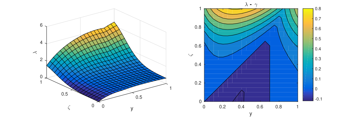
Appendix C Supplementary material
This part of the Appendix refers to video files of the simulation scenarios in Experiments 4, 4, and 4 performed using the randomly-structured ECM initial conditions (4.2). The videos are available at https://github.com/nklb/multi-taxis-supplementary and can be downloaded using the links below. We refer to the corresponding sections of the manuscript for thorough discussions of the experiments.