跳到论文正文
W Papers独立论文阅读器 arXiv:2005.01417 论文正文 计算阅读时间 · 0%
引用这篇论文根据当前论文元数据生成,正式投稿前建议核对。


License: arXiv.org perpetual non-exclusive license
arXiv:2005.01417v3 [math.ST] 26 Mar 2021

Bootstrapping Persistent Betti Numbers
and Other Stabilizing Statistics

Benjamin Roycraft label=e1 Email: [    mark]btroycraft@ucdavis.edu    Johannes Krebs label=e2 Email: [    mark]krebs@uni-heidelberg.de    Wolfgang Polonik label=e3 Email: [    mark]wpolonik@ucdavis.edu Address: Department of Statistics, University of California, Davis, One Shields Avenue, 95616, USA Address: Institute for Applied Mathematics, Heidelberg University, Im Neuenheimer Feld 205, 69120 Heidelberg, Germany Affiliation: UC Davis and Heidelberg University
Abstract

The present contribution investigates multivariate bootstrap procedures for general stabilizing statistics, with specific application to topological data analysis. Existing limit theorems for topological statistics prove difficult to use in practice for the construction of confidence intervals, motivating the use of the bootstrap in this capacity. However, the standard nonparametric bootstrap does not directly provide for asymptotically valid confidence intervals in some situations. A smoothed bootstrap procedure, instead, is shown to give consistent estimation in these settings. The present work relates to other general results in the area of stabilizing statistics, including central limit theorems for functionals of Poisson and Binomial processes in the critical regime. Specific statistics considered include the persistent Betti numbers of Čech and Vietoris-Rips complexes over point sets in ℝd\mathbb{R}^{d}, along with Euler characteristics, and the total edge length of the kk-nearest neighbor graph. Special emphasis is made throughout to weakening the necessary conditions needed to establish bootstrap consistency. In particular, the assumption of a continuous underlying density is not required. A simulation study is provided to assess the performance of the smoothed bootstrap for finite sample sizes, and the method is further applied to the cosmic web dataset from the Sloan Digital Sky Survey (SDSS). Source code is available at github.com/btroycraft/stabilizing_statistics_bootstrap.

Keywords: 
Persistent homology,
keywords
[class=MSC2010]
keywords
††email: e1,e3††email: e2

, and

1 Introduction

In recent years, a multitude of topological statistics have been developed to describe and analyze the structure of data, achieving notable success. These methods have seen application in astrophysics [1, 41, 42, 43], cancer genomics [3, 21, 11], medical imaging [18], materials science [29], fluid dynamics [30] and chemistry [52], and other wide ranging fields.

The use of simplicial complexes to summarize the geometric and topological properties of data culminates in the techniques of persistent homology. Summary statistics based on persistent homology, persistent Betti numbers, persistence diagrams, and derivatives thereof effectively extract essential topological properties from point cloud data. A broad introduction to the methods of topological data analysis can be found in [51, 15].

While the use of such statistics has seen wide success, very little is currently known about the statistical properties of these topological summaries. An initial attempt at statistical analysis using persistent homology can be seen in [10], with the later introduction of persistence landscapes in [9]. Likewise, central limit theorems have been developed for persistence landscapes [13], Betti numbers [54] and persistent Betti numbers [27, 31] under a variety of asymptotic settings. However, the form of these results is insufficient to provide for valid confidence intervals.

In the construction of asymptotically valid confidence intervals, subsampling and bootstrap estimation have proven successful. In [23], various techniques are given for constructing confidence sets for persistence diagrams and derived statistics, including persistence diagrams generated from sublevel sets of the density function, as well as for the Čech and Vietoris-Rips complexes of data constrained to a manifold embedded in ℝd\mathbb{R}^{d}. In [13, 14], bootstrap consistency is established very generally for persistence landscapes drawn from independently generated point clouds in ℝd\mathbb{R}^{d}, assuming that the number of independent samples is allowed to grow.

However, even with these recent developments, the available techniques for constructing confidence sets using topological statistics remain severely limited. The bootstrap has proven one of the only effective tools, however the theoretical properties of bootstrap estimation applied to topological statistics are not well understood. For the large-sample asymptotic regime in particular, results are largely nonexistent.

The goal of this work is to provide the foundational theory for the bootstrap in this area. Here the validity of the bootstrap in the multivariate setting is established, a key step towards an eventual process-level result. However, the latter remains a significant technical hurdle. While motivated primarily by application to topological data analysis, the results presented here apply much more generally over a class of stabilizing statistics. For an additional application, we show convergence for the bootstrap applied to the total edge length of the kk-nearest neighbor graph.

We also analyze the large-sample asymptotic properties of the bootstrap applied to the Čech and Vietoris-Rips complexes directly, where the underlying point cloud is a sample drawn from a common distribution on ℝd\mathbb{R}^{d}. In particular, we will show that the standard nonparametric bootstrap can fail to provide asymptotically valid confidence intervals directly in some cases. Via a smoothed bootstrap, however, we will construct multivariate confidence intervals for the mean persistent Betti number, which lie in bijection with the corresponding persistence diagram.

As defined in [38], a statistic stabilizes if the change in the function value induced by addition of new points to the underlying sample is at most locally determined. Applications of stabilization have allowed for the development of central limit theorems for several topological statistics. [54] show that Betti numbers exhibit the stabilization property, and provide a central limit theorem for Betti numbers derived from a homogenous Poisson process with unit intensity. [27] considers persistent Betti numbers in the homogenous Poisson process case with arbitrary intensity. Most recently [31] established multivariate central limit theorems for persistent Betti numbers with an underlying point cloud coming from either a nonhomogenous Poisson or binomial process. For the results in the present contribution, we draw significant inspiration from this most recent work.

An application of our general consistency result is made to the persistent Betti numbers of a class of distance-based simplicial complexes, including the Čech and Vietoris-Rips complexes. Throughout this work, a special focus is given towards weakening the necessary assumptions compared to previous results. Specifically, the theorems presented here apply for distributions with unbounded support, unbounded density, and possible discontinuities. We assume only a bound for the LpL_{p}-norm of the underlying sampling density.

For the first half of this paper, we focus on the theory of bootstrap estimation applied to stabilizing statistics. In Section 2 we will introduce the concept of stabilization and establish intermediate technical results in this context. We then present our general bootstrap consistency theorem.

In the second half, we introduce the main topological and geometric statistics of interest, applying the theory presented in the previous sections. In Section 3 we connect the general theory to the specific case of persistent homology and related statistics. Towards this end, we give a short introduction to simplicial complexes and persistent homology. In Section 4, the stabilization properties of persistent Betti numbers are analyzed, along with the Euler characteristic, for general classes of distance-based simplicial complexes. We establish bootstrap consistency in the large-sample limit for each of these statistics, as well as for the total edge length of the kk-nearest neighbor graph. In Section 5 we provide several simulations demonstrating the finite-sample properties of the smoothed bootstrap applied to persistent Betti numbers. Finally, Section 6 illustrates the utility of the smoothed bootstrap with an application to a cosmic web dataset from the Sloan Digital Sky Survey (SDSS) [5]. Source code for the computational sections is available at github.com/btroycraft/stabilizing_statistics_bootstrap [44].

Appendix A gives an investigation of several altered problem settings in which precise stabilization properties may be derived. The proofs for all results can be found in Appendix B. Functionals considered include the “BB-bounded” persistent Betti numbers and the “qq-truncated” Euler characteristic.

2 Stabilizing Statistics

2.1 Central Limit Theorems for Stabilizing Statistics

Before proving bootstrap convergence, we give a brief overview of the existing work regarding stabilizing statistics. For the precise definitions used throughout this paper, see Section 2.2.

In the seminal work of [38], the chief objects of study are real valued functionals applied over point sets in ℝd\mathbb{R}^{d}. It is here that a stabilization property was first defined, and used to show central limit theorems for certain types of geometric functionals, including the length of the kk-nearest neighbor graph and the number of edges in the sphere of influence graph. This initial work distilled two properties key to showing central limit theorems for geometric functionals. First is the stabilization property, and second is a moment bound. In short, we say that a functional ψ\psi stabilizes if the cost of adding an additional point, or a set of points, to the point cloud varies only on a bounded region. Specific definitions differ by context.

In [38], the authors distinguish between two data generating regimes. First, results are shown for a homogenous Poisson process over ℝd\mathbb{R}^{d}. Alternatively, a binomial process is considered, being equivalent to a sample of fixed size from an appropriate probability distribution. Here, the functional under consideration is restricted to a bounded domain BnB_{n} of volume nn, where nn is allowed to increase. In this initial work, only homogenous Poisson processes and uniform binomial sampling are considered. In [39], a similar framework is used to establish laws of large numbers for graph-based functionals, including the number of connected components in the minimum spanning tree. Further quantitative refinements on the general central limit theorems for stabilizing statistics are shown in [32], [33], and [34].

As pertains to topological statistics, an initial central limit theorem for Betti numbers (see Section 3.2 for definitions) was shown in [54], establishing so-called weak stabilization for Betti numbers in the homogenous Poisson and uniform Binomial sampling settings. There an alternative set-up is being used where the domain is kept fixed, while the filtration parameter is decreasing to zero. A similar result for persistent Betti numbers is given in [27].

Finally, [31] establishes multivariate central limit theorems for persistent Betti numbers under a flexible sampling setting. Here, a nonhomogeneous Poisson or binomial process is generated again over a growing domain with fixed filtration radii.

With these central limit theorem results, the stabilization property plays a central role in understanding the asymptotic behavior for wide classes of geometric and topological functionals. Unfortunately, as a reoccurring trend, explicit forms for the asymptotic normal distributions are unavailable or computationally intractable. In this work it is shown how a smoothed bootstrap procedure allows for consistent estimation of these inaccessible limiting distributions, and thus for any subsequent inference derived therefrom.

Further, the bootstrap convergence results shown in this paper apply even more broadly, given that the necessary assumptions are much weaker than normally used to establish central limit theorems. To the best of our knowledge, it is not known whether there exist stabilizing statistics which exhibit a non-normal limit, but our convergence results apply equally for any distributional limit.

2.2 Stabilization

Here, we extend and rephrase existing definitions found in [38], [39], [54], and [31] to provide a more general and consistent statistical framework. Let 𝒳⁡(ℝd)\mathcal{X}\left({\mathbb{R}^{d}}\right) denote the space consisting of multisets drawn from ℝd\mathbb{R}^{d} with no accumulation points, with the further restriction that no point in a given multiset may be counted more than finitely often. Any locally-finite point process on ℝd\mathbb{R}^{d} can be represented as a random element of 𝒳⁡(ℝd)\mathcal{X}\left({\mathbb{R}^{d}}\right). Let 𝒳~​(ℝd)⊂𝒳⁡(ℝd)\tilde{\mathcal{X}}\left({\mathbb{R}^{d}}\right)\subset\mathcal{X}\left({\mathbb{R}^{d}}\right) contain the finite multisets drawn from ℝd\mathbb{R}^{d} and ψ:𝒳~​(ℝd)→ℝ\psi\colon\tilde{\mathcal{X}}\left({\mathbb{R}^{d}}\right)\to\mathbb{R} be a measurable function. Furthermore, for S,T∈𝒳~​(ℝd)S,T\in\tilde{\mathcal{X}}\left({\mathbb{R}^{d}}\right) define the addition cost of TT to SS as D⁡(S,ψ,T):=ψ⁡(S∪T)−ψ⁡(S)D\left({S;\psi,T}\right):=\psi\left({S\cup T}\right)-\psi\left({S}\right). When T={z}T=\left\{z\right\} consists of a single point, we call Dz​(S,ψ):=D⁡(S,ψ,{z})D_{z}\left({S;\psi}\right):=D\left({S;\psi,\left\{z\right\}}\right) an add-one cost or the add-zz cost.

Broadly, we say that ψ\psi stabilizes if the addition cost of a given TT varies only on a bounded region. In the preceding literature, the terms “strong” and “weak” stabilization are very often used, with precise definitions changing based on circumstance. In the interest of providing more explanatory and specific terminology, we propose the following definitions.

Seen below, almost-sure and locally-determined almost-sure stabilization (see Definitions 2.4 and 2.5) correspond, respectively, to Definitions 3.1 and 2.1 in [38]. Here we have generalized by accounting for possible measurability issues, however the definitions are essentially equivalent. Let Bz​(r)B_{z}\left({r}\right) denote the closed Euclidean ball centered at z∈ℝdz\in\mathbb{R}^{d} with radius rr. For convenience, the dependence on ψ\psi and TT is implicit in each of the following.

Definition 2.1 (Terminal Addition Cost).

D∞:𝒳⁡(ℝd)→ℝD^{\infty}\colon\mathcal{X}\left({\mathbb{R}^{d}}\right)\rightarrow\mathbb{R} is a terminal addition cost centered at z∈ℝdz\in\mathbb{R}^{d} if D∞​(S)=liml→∞D⁡(S∩Bz​(l))D^{\infty}\left({S}\right)=\lim_{l\rightarrow\infty}D\left({S\cap B_{z}\left({l}\right)}\right) for any S∈𝒳⁡(ℝd)S\in\mathcal{X}\left({\mathbb{R}^{d}}\right) such that the limit exists.

For a finite multiset S∈𝒳~​(ℝd)S\in\tilde{\mathcal{X}}\left({\mathbb{R}^{d}}\right), the terminal addition cost centered at z∈ℝdz\in\mathbb{R}^{d} is D∞​(S)=D​(S)D^{\infty}\left({S}\right)=D\left({S}\right), because no further changes to the addition cost may occur once S∩Bz​(a)S\cap B_{z}\left({a}\right) contains all of SS. This does not hold for infinite multisets, motivating a separate definition. In the special case where T={z}T=\left\{z\right\} is a singleton at the centerpoint, the notation D∞=Dz∞D^{\infty}=D_{z}^{\infty} may be used, and will be seen throughout the remaining sections of the paper.

Definition 2.2 (Stabilization in Probability).

For 𝐒\mathbf{S} a point process taking value in 𝒳⁡(ℝd)\mathcal{X}\left({\mathbb{R}^{d}}\right), ψ\psi stabilizes on 𝐒\mathbf{S} in probability if there exists a center point z∈ℝdz\in\mathbb{R}^{d} and a terminal addition cost D∞D^{\infty} for ψ\psi such that

liml→∞ℙ∗[D(𝐒∩Bz(l))≠D∞(𝐒)]=0.\lim_{l\rightarrow\infty}\mathbb{P}^{*}\left[{D\left({\mathbf{S}\cap B_{z}\left({l}\right)}\right)\neq D^{\infty}\left({\mathbf{S}}\right)}\right]=0. (2.1)

Here ℙ∗\mathbb{P}^{*} denotes the outer probability of a set. Stabilization is said to occur in probability because, for any sequence of non-negative radii (li)i∈ℕ\left({l_{i}}\right)_{i\in\mathbb{N}} such that li→∞l_{i}\rightarrow\infty, D⁡(𝐒∩Bz​(li))​→𝑝​D∞​(𝐒)D\left({\mathbf{S}\cap B_{z}\left({l_{i}}\right)}\right)\overset{p}{\rightarrow}D^{\infty}\left({\mathbf{S}}\right) whenever both quantities are measurable. D∞D^{\infty} is unique up to a null set in this case. Stabilization in probability is difficult to show directly for many functions of interest. As such, we have the following:

Definition 2.3 (Radius of Stabilization).

ρ:𝒳⁡(ℝd)→[0,∞]\rho\colon\mathcal{X}\left({\mathbb{R}^{d}}\right)\to\left[{0,\infty}\right] is a radius of stabilization for ψ\psi centered at z∈ℝdz\in\mathbb{R}^{d} if, for any S∈𝒳⁡(ℝd)S\in\mathcal{X}\left({\mathbb{R}^{d}}\right) and l∈ℝl\in\mathbb{R} such that ρ⁡(S)≤l<∞\rho\left({S}\right)\leq l<\infty,

D⁡(S∩Bz​(l))=D⁡(S∩Bz​(ρ⁡(S))).D\left({S\cap B_{z}\left({l}\right)}\right)=D\left({S\cap B_{z}\left({\rho\left({S}\right)}\right)}\right). (2.2)

D∞​(S):=D⁡(S∩Bz​(ρ⁡(S)))D^{\infty}\left({S}\right):=D\left({S\cap B_{z}\left({\rho\left({S}\right)}\right)}\right) is a valid terminal addition cost. In the case where liml→∞D⁡(S∩Bz​(l))\\ \lim_{l\rightarrow\infty}D\left({S\cap B_{z}\left({l}\right)}\right) does not exist, ρ⁡(S)=∞\rho\left({S}\right)=\infty necessarily, with the stabilization criterion satisfied vacuously. As with the terminal addition cost, when T={z}T=\left\{z\right\} we denote ρ=ρz\rho=\rho_{z}.

In general, for any ψ\psi there exists a unique minimal radius of stabilization, defined as the pointwise minimum over all such radii sharing the same centerpoint. This minimum exists because ψ​(S∩Bz​(l))\psi\left({S\cap B_{z}\left({l}\right)}\right) is piecewise constant in 0≤l<∞0\leq l<\infty, changing value only when a new point of SS is added, and because SS has no accumulation points.

Definition 2.4 (Stabilization Almost Surely).

For 𝐒\mathbf{S} a point process taking value in 𝒳⁡(ℝd)\mathcal{X}\left({\mathbb{R}^{d}}\right), ψ\psi stabilizes on 𝐒\mathbf{S} almost surely if there exists a radius of stabilization ρ:𝒳⁡(ℝd)→[0,∞]\rho\colon\mathcal{X}\left({\mathbb{R}^{d}}\right)\rightarrow\left[{0,\infty}\right] for ψ\psi centered at z∈ℝdz\in\mathbb{R}^{d} such that

limL→∞ℙ∗[ρ(𝐒)>L]=0.\lim_{L\rightarrow\infty}\mathbb{P}^{*}\left[{\rho\left({\mathbf{S}}\right)>L}\right]=0. (2.3)

Mirroring our previous terminology, we say stabilization occurs almost surely because, for any sequence of nonnegative radii (li)i∈ℕ\left({l_{i}}\right)_{i\in\mathbb{N}} such that li→∞l_{i}\rightarrow\infty, D⁡(𝐒∩Bz​(li))​→a.s.​D∞​(𝐒)=D⁡(𝐒∩Bz​(ρ⁡(𝐒)))D\left({\mathbf{S}\cap B_{z}\left({l_{i}}\right)}\right)\overset{a.s.}{\rightarrow}D^{\infty}\left({\mathbf{S}}\right)=D\left({\mathbf{S}\cap B_{z}\left({\rho\left({\mathbf{S}}\right)}\right)}\right) whenever both quantities are measurable. Here we use outer probability, because a radius of stabilization may not be a measurable function, specifically considering the unique minimal radius. Almost sure stabilization implies stabilization in probability, as shown in the following.

Proposition 2.1.

For 𝐒\mathbf{S} a simple point process taking values in 𝒳⁡(ℝd)\mathcal{X}\left({\mathbb{R}^{d}}\right), let ψ\psi stabilize on 𝐒\mathbf{S} almost surely. Then ψ\psi stabilizes on 𝐒\mathbf{S} in probability.

For our proof techniques, it is often necessary to compare the stabilization properties of a function over a range of related point processes. For example, corresponding binomial, Poisson, and Cox processes can be shown to have essentially equivalent local properties, while differing globally. As defined in Definition 2.3, a given radius of stabilization could feasibly show completely different behavior on each process type. This motivates the following:

Definition 2.5 (Locally Determined Radius of Stabilization).

The radius of stabilization ρ\rho centered at z∈ℝdz\in\mathbb{R}^{d} is locally determined if for any S,T∈𝒳⁡(ℝd)S,T\in\mathcal{X}\left({\mathbb{R}^{d}}\right)

T∩Bz​(ρ⁡(S))=S∩Bz​(ρ⁡(S))⟹ρ⁡(T)=ρ⁡(S).T\cap B_{z}\left({\rho\left({S}\right)}\right)=S\cap B_{z}\left({\rho\left({S}\right)}\right)\implies\rho\left({T}\right)=\rho\left({S}\right).

With the local-determination criterion from Definition 2.5, we can assure that stabilization must occur simultaneously on any two point processes which are locally equivalent. As in the non-locally-determined case, there exists a unique minimal locally-determined radius of stabilization:

Proposition 2.2.

For ℛ\mathcal{R} the space of locally-determined radii of stabilization for ψ\psi centered at z∈ℝdz\in\mathbb{R}^{d}, let ρ∗:𝒳⁡(ℝd)→[0,∞]\rho^{*}\colon\mathcal{X}\left({\mathbb{R}^{d}}\right)\rightarrow\left[{0,\infty}\right] such that ρ∗​(S)=infρ∈ℛρ⁡(S)\rho^{*}\left({S}\right)=\inf_{\rho\in\mathcal{R}}\rho\left({S}\right). Then ρ∗\rho^{*} is a locally determined radius of stabilization for ψ\psi centered at zz.

2.3 Technical Results

In all of the following, 𝒫⁡(ℝd)\mathcal{P}\left({\mathbb{R}^{d}}\right) denotes the set of probability distributions over ℝd\mathbb{R}^{d}. Y1,…,Yn​∼iid​GY_{1},...,Y_{n}\overset{\text{iid}}{\sim}G is a sample from G∈𝒫⁡(ℝd)G\in\mathcal{P}\left({\mathbb{R}^{d}}\right) and Y′∼GY^{\prime}\sim G an independent copy. Let 𝐘n={Yi}i=1n\mathbf{Y}_{n}=\left\{Y_{i}\right\}_{i=1}^{n} be the induced multiset. This definition may be simply denoted by 𝐘n:={Yi}i=1n​∼iid​G\mathbf{Y}_{n}:=\left\{Y_{i}\right\}_{i=1}^{n}\overset{\text{iid}}{\sim}G. For a measurable function ψ:𝒳~​(ℝd)→ℝ\psi\colon\tilde{\mathcal{X}}\left({\mathbb{R}^{d}}\right)\rightarrow\mathbb{R}, define the following conditions:

  1. (E1)

    For a given 𝒞⊆𝒫⁡(ℝd)\mathcal{C}\subseteq\mathcal{P}\left({\mathbb{R}^{d}}\right) and some a>2a>2, there exists Ea<∞E_{a}<\infty such that

    supG∈𝒞supn∈ℕ𝔼⁡[|ψ⁡(nd​(𝐘n∪{Y′}))−ψ⁡(nd​𝐘n)|a]≤Ea.\sup_{G\in\mathcal{C}}\sup_{n\in\mathbb{N}}\mathbb{E}\left[{\left|{\psi\left({\sqrt[d]{n}\left({\mathbf{Y}_{n}\cup\left\{Y^{\prime}\right\}}\right)}\right)-\psi\left({\sqrt[d]{n}\mathbf{Y}_{n}}\right)}\right|^{a}}\right]\leq E_{a}. (2.4)
  2. (E2)

    For some a>2a>2 and R>0R>0, there exist Ua>0U_{a}>0 and ua>1u_{a}>1 satisfying the following property: For any S∈𝒳~​(ℝd)S\in\tilde{\mathcal{X}}\left({\mathbb{R}^{d}}\right) and y∈ℝdy\in\mathbb{R}^{d},

    |ψ⁡(S∪{y})−ψ⁡(S)|a≤Ua​(1+#​{S∩By​(R)}ua).\left|{\psi\left({S\cup\left\{y\right\}}\right)-\psi\left({S}\right)}\right|^{a}\leq U_{a}\left({1+\#\left\{S\cap B_{y}\left({R}\right)\right\}^{u_{a}}}\right). (2.5)

(E1) requires a moment bound that holds uniformly in the sample size and distribution G∈𝒞G\in\mathcal{C}. Clearly, if (E1) is satisfied for 𝒞\mathcal{C}, it is also satisfied for any subset of 𝒞\mathcal{C}. In the context of the topological statistics considered in this work, (E1) is primarily useful for proof purposes, and is mainly established via (E2) (See Lemma 2.3). However, as will be seen with the case of the kk-nearest neighbor graph, Corollary 4.6, there exist useful statistics which do not conform to (E2), and the more general condition must be used. (E1) is related to the “uniform bounded moments” condition, Definition 2.2 in [38]. Our version has been suitably generalized, the original definition considering only a=4a=4. Let 𝒞p,M​(ℝd)\mathcal{C}_{p,M}\left({\mathbb{R}^{d}}\right) denote the class of probability distributions G∈𝒫⁡(ℝd)G\in\mathcal{P}\left({\mathbb{R}^{d}}\right) admitting a density gg such that ‖g‖p≤M\|g\|_{p}\leq M. We have the following:

Lemma 2.3.

For p>2p>2, let ψ\psi satisfy (E2) with ua≤p−1u_{a}\leq p-1 for some a>2a>2. Then for any M<∞M<\infty, ψ\psi satisfies (E1) for 𝒞p,M​(ℝd)\mathcal{C}_{p,M}\left({\mathbb{R}^{d}}\right).

For dTVd_{\text{TV}} the total variation distance between probability distributions and BF​(ϵ,dTV)B_{F}(\epsilon,d_{\text{TV}}) the closed ϵ\epsilon-neighborhood of FF under dTVd_{\text{TV}}, we have the following stabilization conditions:

  1. (S1)

    For a given 𝒞⊆𝒫⁡(ℝd)\mathcal{C}\subseteq\mathcal{P}\left({\mathbb{R}^{d}}\right), F∈𝒞F\in\mathcal{C}, b>0b>0, and some (lϵ)ϵ>0\left({l_{\epsilon}}\right)_{\epsilon>0} such that limϵ→0lϵ​ϵb=0\lim_{\epsilon\rightarrow 0}l_{\epsilon}\epsilon^{b}=0, as ϵ→0,\epsilon\to 0,

    supG∈𝒞∩BF​(ϵ,dTV)supn∈ℕℙ[Dnd​Y′((nd𝐘n)∩Bnd​Y′(lϵ))≠Dnd​Y′(nd𝐘n)]→0.\sup_{G\in\mathcal{C}\cap B_{F}\left({\epsilon;d_{\text{TV}}}\right)}\sup_{n\in\mathbb{N}}\mathbb{P}\left[{D_{\sqrt[d]{n}Y^{\prime}}\left({\left({\sqrt[d]{n}\mathbf{Y}_{n}}\right)\cap B_{\sqrt[d]{n}Y^{\prime}}\left({l_{\epsilon}}\right)}\right)\neq D_{\sqrt[d]{n}Y^{\prime}}\left({\sqrt[d]{n}\mathbf{Y}_{n}}\right)}\right]\to 0.
  2. (S2)

    For G∈𝒫⁡(ℝd)G\in\mathcal{P}\left({\mathbb{R}^{d}}\right), there exist locally-determined radii of stabilization (ρz)z∈ℝd\left({\rho_{z}}\right)_{z\in\mathbb{R}^{d}} for ψ\psi satisfying

    limL→∞supn∈ℕℙ∗[ρnd​Y′(nd𝐘n)>L]=0.\lim_{L\to\infty}\sup_{n\in\mathbb{N}}\mathbb{P}^{*}\left[{\rho_{\sqrt[d]{n}Y^{\prime}}\left({\sqrt[d]{n}\mathbf{Y}_{n}}\right)>L}\right]=0. (2.6)

(S1) and (S2) can be summarized as uniform stabilization conditions, either in probability or almost surely. (S1) as stated is a technical condition mainly serving to weaken the necessary conditions providing for bootstrap consistency. As such, we have the following lemma linking (S1) and (S2).

Lemma 2.4.

Let ψ\psi satisfy (S2) for F∈Cp,M​(ℝd)F\in C_{p,M}\left({\mathbb{R}^{d}}\right). Then ψ\psi satisfies (S1) for Cp,M​(ℝd)C_{p,M}\left({\mathbb{R}^{d}}\right), FF, b=(p−2)/(d⁡(p−1))b=\left({p-2}\right)/\left({d\left({p-1}\right)}\right), and any (lϵ)ϵ>0\left({l_{\epsilon}}\right)_{\epsilon>0} such that limϵ→0lϵ​ϵ(p−2)/(d⁡(p−1))=0\lim_{\epsilon\rightarrow 0}l_{\epsilon}\epsilon^{\left({p-2}\right)/\left({d\left({p-1}\right)}\right)}=0 and limϵ→0lϵ=∞\lim_{\epsilon\rightarrow 0}l_{\epsilon}=\infty.

We can often greatly simplify the addition costs and radii of stabilization required in (S1) and (S2). For example, given a translation-invariant function ψ\psi and any D0D_{0}, ρ0\rho_{0} for ψ\psi centered at 00, corresponding quantities can be constructed for any other center point. For z∈ℝdz\in\mathbb{R}^{d}, Dz:𝒳⁡(ℝd)→ℝD_{z}\colon\mathcal{X}\left({\mathbb{R}^{d}}\right)\rightarrow\mathbb{R} where Dz​(S)=D0​(S−z)D_{z}\left({S}\right)=D_{0}\left({S-z}\right) is an add-zz cost for ψ\psi centered at zz. Likewise ρz:𝒳⁡(ℝd)→[0,∞]\rho_{z}\colon\mathcal{X}\left({\mathbb{R}^{d}}\right)\rightarrow\left[{0,\infty}\right] where ρz​(S)=ρ0​(S−z)\rho_{z}\left({S}\right)=\rho_{0}\left({S-z}\right) is a radius of stabilization for ψ\psi centered at zz. In the following, 𝐏λ\mathbf{P}_{\lambda} denotes a homogeneous Poisson process on ℝd\mathbb{R}^{d} with intensity λ\lambda.

Lemma 2.5.

Let F∈Cp,MF\in C_{p,M} with p>2p>2 and M<∞M<\infty. Let ρ0\rho_{0} be a locally-determined radius of stabilization for ψ\psi centered at 00. Suppose that for any given a,b∈(0,∞)a,b\in\left({0,\infty}\right), and δ>0\delta>0, there exists an La,b,δ<∞L_{a,b,\delta}<\infty and a measurable set Aa,b,δA_{a,b,\delta} with ρ0−1​((La,b,δ,∞])⊆Aa,b,δ\rho_{0}^{-1}\left({\left(L_{a,b,\delta},\infty\right]}\right)\subseteq A_{a,b,\delta} such that

supλ∈[a,b]ℙ∗[ρ0(𝐏λ)>La,b,δ]≤supλ∈[a,b]ℙ[𝐏λ∈Aa,b,δ]≤δ.\sup_{\lambda\in\left[{a,b}\right]}\mathbb{P}^{*}\left[{\rho_{0}\left({\mathbf{P}_{\lambda}}\right)>L_{a,b,\delta}}\right]\leq\sup_{\lambda\in\left[{a,b}\right]}\mathbb{P}\left[{\mathbf{P}_{\lambda}\in A_{a,b,\delta}}\right]\leq\delta. (2.7)

Then for any δ>0\delta>0 there exists an nδ<∞n_{\delta}<\infty and Lδ<∞L_{\delta}<\infty such that

supn≥nδℙ∗[ρ0(𝐗n−X′)>Lδ]≤δ.\sup\limits_{n\geq n_{\delta}}\mathbb{P}^{*}\left[{\rho_{0}\left({\mathbf{X}_{n}-X^{\prime}}\right)>L_{\delta}}\right]\leq\delta. (2.8)

Lemma 2.5 provides a convenient tool for “de-Poissonizing” a locally-determined radius of stabilization. Often it is easier to show stabilization properties for a homogeneous Poisson process than for a binomial process directly. Lemma 2.5 allows for the extension of homogeneous Poisson results to the binomial setting, as is required for Lemma 4.1 and Corollary 4.6. Note that the conclusion is not the same as the statement of (S1), only applying for n≥nδn\geq n_{\delta}. Some extra effort is required for the conclusion to hold for all n∈ℕn\in\mathbb{N}, depending on the specifics of the function ψ\psi considered. We come to the following important proposition, the main supporting result for our general bootstrap consistency theorem, Theorem 2.7.

Proposition 2.6.

For p>2p>2 and M<∞M<\infty, let ψ\psi satisfy (E1) and (S1) for 𝒞p,M​(ℝd)\mathcal{C}_{p,M}\left({\mathbb{R}^{d}}\right), F∈𝒞p,M​(ℝd)F\in\mathcal{C}_{p,M}\left({\mathbb{R}^{d}}\right), and some a>2a>2. Then for any G∈𝒞p,M​(ℝd)∩BF​(ϵ,dTV)G\in\mathcal{C}_{p,M}\left({\mathbb{R}^{d}}\right)\cap B_{F}\left({\epsilon,d_{\text{TV}}}\right), there exist iid coupled random variables ((Xi,Yi))i∈ℕ\left({\left({X_{i},Y_{i}}\right)}\right)_{i\in\mathbb{N}} such that 𝐗n={Xi}i=1n​∼iid​F\mathbf{X}_{n}=\left\{X_{i}\right\}_{i=1}^{n}\overset{\text{iid}}{\sim}F, 𝐘n={Yi}i=1n​∼iid​G\mathbf{Y}_{n}=\left\{Y_{i}\right\}_{i=1}^{n}\overset{\text{iid}}{\sim}G, and

supn∈ℕVar⁡V​a​r​[1n​(ψ⁡(nd​𝐗n)−ψ⁡(nd​𝐘n))]≤γϵ.\sup_{n\in\mathbb{N}}\.Var\left[{\frac{1}{\sqrt{n}}\left({\psi\left({\sqrt[d]{n}\mathbf{X}_{n}}\right)-\psi\left({\sqrt[d]{n}\mathbf{Y}_{n}}\right)}\right)}\right]\leq\gamma_{\epsilon}. (2.9)

The value γϵ\gamma_{\epsilon} does not depend on GG and satisfies limϵ→0γϵ=0\lim_{\epsilon\rightarrow 0}\gamma_{\epsilon}=0.

For any two distributions ℒ1\mathcal{L}_{1} and ℒ2\mathcal{L}_{2} over ℝ\mathbb{R}, we may define the 2-Wasserstein distance between ℒ1\mathcal{L}_{1} and ℒ2\mathcal{L}_{2} as

W2​(ℒ1,ℒ2):=infU∼ℒ1,V∼ℒ2𝔼⁡[(U−V)2]W_{2}\left({\mathcal{L}_{1},\mathcal{L}_{2}}\right):=\sqrt{\inf_{U\sim\mathcal{L}_{1},V\sim\mathcal{L}_{2}}\mathbb{E}\left[{\left({U-V}\right)^{2}}\right]} (2.10)

where it is assumed that UU and VV follow a joint distribution with marginals ℒ1\mathcal{L}_{1} and ℒ2\mathcal{L}_{2}. For ℒ\mathcal{L} denoting the law or distribution of a random variable, the variance given in the conclusion of Proposition 2.6 bounds above

W22​(ℒ⁡{1n​(ψ⁡(nd​𝐗n)−𝔼⁡[ψ⁡(nd​𝐗n)])}CLOSE,\displaystyle W_{2}^{2}\Biggl(\mathcal{L}\left\{\frac{1}{\sqrt{n}}\left({\psi\left({\sqrt[d]{n}\mathbf{X}_{n}}\right)-\mathbb{E}\left[{\psi\left({\sqrt[d]{n}\mathbf{X}_{n}}\right)}\right]}\right)\right\}, (2.11)
ℒ{1n(ψ(nd𝐘n)−𝔼[ψ(nd𝐘n)])}).\displaystyle\qquad\qquad\qquad\qquad\mathcal{L}\left\{\frac{1}{\sqrt{n}}\left({\psi\left({\sqrt[d]{n}\mathbf{Y}_{n}}\right)-\mathbb{E}\left[{\psi\left({\sqrt[d]{n}\mathbf{Y}_{n}}\right)}\right]}\right)\right\}\Biggl).

Consequently, Proposition 2.6 shows that this W2W_{2} distance can be made arbitrarily small uniformly over a neighborhood of distributions around FF. An appropriately smoothed empirical distribution falls within such a small neighborhood with high probability, given sufficiently large sample sizes.

Furthermore, it can be seen that Proposition 2.6 extends directly to finite sums. Given any (Ai)i=1k\left({A_{i}}\right)_{i=1}^{k} and (Bi)i=1k\left({B_{i}}\right)_{i=1}^{k}, we have that Var⁡V​a​r​[∑i=1kAi−∑i=1kBi]≤k​∑i=1kVar⁡V​a​r​[Ai−Bi]\.Var\left[{\sum_{i=1}^{k}A_{i}-\sum_{i=1}^{k}B_{i}}\right]\leq k\sum_{i=1}^{k}\.Var\left[{A_{i}-B_{i}}\right]. Thus, if the conclusion of Proposition 2.6 holds for any finite set of functions, (ψi)i=1k\left({\psi_{i}}\right)_{i=1}^{k}, it also holds for ∑i=1kψi\sum_{i=1}^{k}\psi_{i}, with rate depending on the worst case ψi\psi_{i}.

It should be noted that (S1) is slightly stronger than necessary to establish Proposition 2.6. As stated, Dnd​Y′​((nd​𝐘n)∩Bnd​Y′​(lϵ))D_{\sqrt[d]{n}Y^{\prime}}\left({\left({\sqrt[d]{n}\mathbf{Y}_{n}}\right)\cap B_{\sqrt[d]{n}Y^{\prime}}\left({l_{\epsilon}}\right)}\right) itself is compared to the terminal add-one cost Dnd​Y′​(nd​𝐘n)D_{\sqrt[d]{n}Y^{\prime}}\left({\sqrt[d]{n}\mathbf{Y}_{n}}\right). As could be useful for some statistics, it is only required that an appropriate bound displays the desired stabilization property, see the provided proof for details.

2.4 Smoothed Bootstrap

The bootstrap is an estimation technique used to construct approximate confidence intervals for a given population parameter. In cases where asymptotic approximations for the sampling distribution of a statistic are inconvenient or unavailable, bootstrap estimation provides a general tool for constructing approximate confidence intervals. Bootstrap estimation is well-studied in the statistical literature, an introduction being provided in [40]. In this section, we will show consistency for a smoothed bootstrap in estimating the limiting distribution of a standardized stabilizing statistic, ψ\psi, in the multivariate setting. We describe the general procedure below:

Let 𝐗n={Xi}i=1n​∼iid​F\mathbf{X}_{n}=\left\{X_{i}\right\}_{i=1}^{n}\overset{\text{iid}}{\sim}F. We estimate the sampling distribution of

1n​(ψ⁡(nd​𝐗n)−𝔼⁡[ψ⁡(nd​𝐗n)])\frac{1}{\sqrt{n}}\left({\psi\left({\sqrt[d]{n}\mathbf{X}_{n}}\right)-\mathbb{E}\left[{\psi\left({\sqrt[d]{n}\mathbf{X}_{n}}\right)}\right]}\right) (2.12)

using a plug-in estimator F^n\hat{F}_{n} for the underlying data distribution FF. In the standard nonparametric bootstrap, we estimate FF by the empirical distribution, giving probability to each unique value of (Xi)i=1n\left({X_{i}}\right)_{i=1}^{n}, proportional to the number of repetitions within 𝐗n\mathbf{X}_{n}. We have the bootstrap statistic

1m​(ψ⁡(md​𝐗m∗)−𝔼⁡[ψ⁡(md​𝐗m∗)|𝐗n]),\frac{1}{\sqrt{m}}\left({\psi\left({\sqrt[d]{m}\mathbf{X}_{m}^{*}}\right)-\mathbb{E}\left[{\psi\left({\sqrt[d]{{m}}\mathbf{X}_{m}^{*}}\right)\big|\mathbf{X}_{n}}\right]}\right), (2.13)

where 𝐗m∗={Xi∗}i=1m​∼iid​F^n|𝐗n\mathbf{X}_{m}^{*}=\left\{X_{i}^{*}\right\}_{i=1}^{m}\overset{\text{iid}}{\sim}\hat{F}_{n}|\mathbf{X}_{n}, conditional on 𝐗n\mathbf{X}_{n}. The sampling distribution of the bootstrap version provides an estimate for the distribution of the original statistic, which in the ideal case converges to the truth in the large-sample limit. Confidence intervals for 𝔼⁡[ψ⁡(nd​𝐗n)]\mathbb{E}\left[{\psi\left({\sqrt[d]{n}\mathbf{X}_{n}}\right)}\right] are then constructed from the bootstrap distribution and ψ⁡(nd​𝐗n)\psi\left({\sqrt[d]{n}\mathbf{X}_{n}}\right).

However, as will be seen in Section 4.1, for some classes of topological statistics the standard bootstrap may not directly replicate the correct sampling distribution asymptotically. Consequently, we instead estimate FF by a smoothed distribution approximation. Such a smoothed bootstrap procedure can be shown to provide consistent estimation, even when the standard nonparametric bootstrap may fail.

For the smoothed bootstrap sampling procedure outlined here, we require that FF has a density ff. Let f^n\hat{f}_{n} be an estimator for the true density with corresponding distribution F^n\hat{F}_{n}, each a function of the sample 𝐗n\mathbf{X}_{n}. Conditional on 𝐗n\mathbf{X}_{n}, we draw bootstrap samples 𝐗m∗\mathbf{X}_{m}^{*} independently from F^n|𝐗n\hat{F}_{n}|\mathbf{X}_{n}. A particular choice of f^n\hat{f}_{n} is given via kernel density estimation. For a kernel function QQ and bandwidth h>0h>0, the kernel density estimator of f⁡(x)f(x) based on the sample (Xi)i=1n\left({X_{i}}\right)_{i=1}^{n} is f^n,h(x):=1/(nhd)∑i=1nQ((x−Xi)/h)\hat{f}_{n,h}\left({x}\right):=1/\left({nh^{d}}\right)\sum_{i=1}^{n}Q\left({\left({x-X_{i}}\right)/h}\right).

In practice, when QQ corresponds to a probability density, the kernel density estimator allows for convenient sampling, as is required for implementation. Generating a sample from f^n,h\hat{f}_{n,h} is equivalent to first drawing from the empirical distribution on 𝐗n\mathbf{X}_{n}, then adding independent noise following the distribution defined by QQ, scaled by the bandwidth hh. Other density estimators, including those using higher-order kernels, may not facilitate efficient sampling. However, the theory established here supports the use of any density estimator which meets the required convergence criteria, computational factors aside. More complicated data-dependent estimators are also possible, falling under a similar sampling framework. See Sections 5 and 6 for specifics on density estimation as pertains to this work from a practical perspective.

We now present our main result. The following theorem establishes consistency for the smoothed bootstrap in the multivariate setting. We give the result for a vector of stabilizing statistics. In the context of the topological statistics introduced in Section 3, this can be the persistent Betti numbers or Euler characteristic evaluated at different filtration parameters.

Theorem 2.7.

Let F∈𝒫⁡(ℝd)F\in\mathcal{P}\left({\mathbb{R}^{d}}\right) with density ff such that ‖f‖p<∞\|f\|_{p}<\infty for some p>2p>2. Furthermore, let FF and f^n\hat{f}_{n} be such that ‖f^n−f‖1→0\|\hat{f}_{n}-f\|_{1}\to 0 and ‖f^n−f‖p→0\|\hat{f}_{n}-f\|_{p}\to 0 in probability (resp. a.s.). Suppose ψ→:𝒳~​(ℝd)→ℝk\vec{\psi}\colon\tilde{\mathcal{X}}\left({\mathbb{R}^{d}}\right)\rightarrow\mathbb{R}^{k} has component functions ψj:𝒳~​(ℝd)→ℝ\psi_{j}\colon\tilde{\mathcal{X}}\left({\mathbb{R}^{d}}\right)\rightarrow\mathbb{R}, 1≤j≤k1\leq j\leq k satisfying (E1) and (S1) for 𝒞p,M​(ℝd)\mathcal{C}_{p,M}\left({\mathbb{R}^{d}}\right), M>‖f‖pM>\|f\|_{p}, FF, and b=(p−2)/(d⁡(p−1))b=\left({p-2}\right)/\left({d\left({p-1}\right)}\right). Then for a sample 𝐗n={Xi}i=1n​∼iid​F\mathbf{X}_{n}=\left\{X_{i}\right\}_{i=1}^{n}\overset{\text{iid}}{\sim}F, (mn)n∈ℕ\left({m_{n}}\right)_{n\in\mathbb{N}} such that limn→∞mn=∞\lim_{n\rightarrow\infty}m_{n}=\infty, a bootstrap sample 𝐗mn∗={Xi∗}i=1mn​∼iid​F^n|𝐗n\mathbf{X}_{m_{n}}^{*}=\left\{X_{i}^{*}\right\}_{i=1}^{m_{n}}\overset{\text{iid}}{\sim}\hat{F}_{n}|\mathbf{X}_{n}, and a multivariate distribution GG,

1n​(ψ→​(nd​𝐗n)−𝔼⁡[ψ→​(nd​𝐗n)])​→𝑑​G\frac{1}{\sqrt{n}}\left({\vec{\psi}\left({\sqrt[d]{n}\mathbf{X}_{n}}\right)-\mathbb{E}\left[{\vec{\psi}\left({\sqrt[d]{n}\mathbf{X}_{n}}\right)}\right]}\right)\overset{d}{\rightarrow}G

if and only if

1mn​(ψ→​(mnd​𝐗mn∗)−𝔼⁡[ψ→​(mnd​𝐗mn∗)|𝐗n])​→𝑑​G​ in probability (resp. a.s.).\frac{1}{\sqrt{{m_{n}}}}\left({\vec{\psi}\left({\sqrt[d]{{m_{n}}}\mathbf{X}_{m_{n}}^{*}}\right)-\mathbb{E}\left[{\vec{\psi}\left({\sqrt[d]{{m_{n}}}\mathbf{X}_{m_{n}}^{*}}\right)\big|\mathbf{X}_{n}}\right]}\right)\overset{d}{\rightarrow}G\text{ in probability (resp. a.s.)}.

Theorem 2.7 establishes the asymptotic validity of bootstrap estimation for a range of stabilizing statistics under fairly mild conditions on the underlying density. However, it should be noted that further restrictions on the density and density estimate may be required to satisfy (E1) and (S1), see Corollary 4.6 for example. The conditions under which ‖f^n,hn−f‖1→0\|\hat{f}_{n,h_{n}}-f\|_{1}\to 0 in probability or a.s. can be found in [20]. Proposition C.1 considers the convergence of ‖f^n,hn−f‖p\|\hat{f}_{n,h_{n}}-f\|_{p}, either in probability or almost surely. This result is outside the main contribution of this paper, but is interesting in its own right. Notably, no conditions are placed on the density ff except ‖f‖p<∞\|f\|_{p}<\infty.

As a point of caution, it is known that kernel density estimators suffer from a curse of dimensionality. The convergence properties of the density estimator f^n\hat{f}_{n} appear implicitly within the necessary assumptions for Theorem 2.7. In particular, diminishing performance can be expected in higher dimensions, as shown by the provided simulations of Section 5.

The above result holds for any choice of mnm_{n} such that limn→∞mn=∞\lim_{n\rightarrow\infty}m_{n}=\infty, and is stated as such for the sake of generality. In practical application, mn=nm_{n}=n is standard, and will be used throughout the simulation and data analysis sections of this paper. However, given that the computational complexity of ψ\psi often grows quickly with nn, using a smaller mnm_{n} could prove more feasible from a computational perspective.

Strictly speaking, convergence to a limiting distribution is not required for the bootstrap to provide asymptotically valid confidence intervals. Proposition 2.6 gives that, with high probability, the smoothed bootstrap and true sampling distributions become close in 22-Wasserstein distance. Provided that the cumulative distribution function Fψ→nF_{\vec{\psi}_{n}} of (ψ→​(nd​𝐗n)−𝔼⁡[ψ→​(nd​𝐗n)])/n(\vec{\psi}\left({\sqrt[d]{n}\mathbf{X}_{n}}\right)-\mathbb{E}[\vec{\psi}\left({\sqrt[d]{n}\mathbf{X}_{n}}\right)])/\sqrt{n} has the property

limδ→0lim supn→∞supx∈ℝd|Fψ→n​(x+δ)−Fψ→n​(x)|→0,\lim_{\delta\rightarrow 0}\limsup_{n\rightarrow\infty}\sup_{x\in\mathbb{R}^{d}}\left|{F_{\vec{\psi}_{n}}\left({x+\delta}\right)-F_{\vec{\psi}_{n}}\left({x}\right)}\right|\to 0, (2.14)

it can be shown that confidence intervals constructed from the bootstrap statistic still achieve the stated confidence level with high probability, given a sufficiently large sample. Convergence to a continuous limiting CDF is just one way of satisfying this condition. However, this extension is unavailable for the topological statistics considered here, as the behavior of the finite sample statistics is currently very poorly understood.

In the later sections, we will show that the necessary moment and stabilization conditions for Theorem 2.7 are satisfied for several specific statistics of interest, chiefly the Euler characteristic and persistent Betti numbers for a class of simplicial complexes.

3 Simplicial Complexes and Persistence Homology

3.1 Simplicial Complexes

Let 𝒦={Kr}r∈ℝ\mathcal{K}=\{K^{r}\}_{r\in\mathbb{R}} be a filtration of simplicial complexes, with Kr⊆KtK^{r}\subseteq K^{t} for r<tr<t. Each complex is a collection of simplices, subsets of the vertex multiset, VV. Here any repeated vertices are considered distinct. For a collection of simplices KK to be a simplicial complex, for any two simplices S⊂VS\subset V and T⊂ST\subset S, S∈KS\in K only if T∈KT\in K. Here a simplex is only included along with all of its subsets. For a given simplicial complex KK, KqK_{q} denotes the subset of KK consisting of all qq-simplices. qq-simplices are those simplices consisting of q+1q+1 vertices. Each qq-simplex is said to have dimension qq. A graph or network refers to a simplicial complex consisting of only 11-simplices (edges) and 00-simplices (vertices).

We will be looking at simplicial complexes constructed over point clouds in ℝd\mathbb{R}^{d}. The two major examples are the Čech and Vietoris-Rips complexes:

KCr​(S)\displaystyle K_{\text{C}}^{r}\left({S}\right) ={σ⊆S:∃z∈ℝd​ s.t. ​‖z−x‖≤r​∀x∈σ}\displaystyle=\left\{\sigma\subseteq S\colon\exists z\in\mathbb{R}^{d}\text{ s.t. }\|z-x\|\leq r\ \forall x\in\sigma\right\} (3.1)
KVRr​(S)\displaystyle K_{\text{VR}}^{r}\left({S}\right) ={σ⊆S:∥x−y∥≤2r∀x,y∈σ}.\displaystyle=\left\{\sigma\subseteq S\colon\|x-y\|\leq 2r\ \forall x,y\in\sigma\right\}. (3.2)

Each of these complexes summarizes the geometric and topological properties within a given point cloud. The Vietoris-Rips complex can be considered a “completion” of the Čech complex, in so much that the Vietoris-Rips complex is the largest simplicial complex with the same edge set as the Čech complex. While the primary motivation for the results given here is application to the Čech and Vietoris-Rips complexes, our main results apply for a range of possible complexes. For example, for computational reasons it is often convenient to limit the number of simplices present within the final complex. As such, we have two approximations, the alpha complex and its completion

Kαr​(S)\displaystyle K_{\alpha}^{r}\left({S}\right) ={σ⊆S:∃z∈ℝd​ s.t. ​‖z−x‖≤r​ and ​‖z−x‖≤‖z−y‖​∀x∈σ​∀y∈S}\displaystyle=\left\{\sigma\subseteq S\colon\exists z\in\mathbb{R}^{d}\text{ s.t. }\|z-x\|\leq r\and\|z-x\|\leq\|z-y\|\ \forall x\in\sigma\ \forall y\in S\right\}
Kα∗r​(S)\displaystyle K_{\alpha^{*}}^{r}\left({S}\right) ={σ⊆S:{x,y}∈Kαr(S)∀x,y∈σ}.\displaystyle=\left\{\sigma\subseteq S\colon\left\{x,y\right\}\in K_{\alpha}^{r}\left({S}\right)\ \forall x,y\in\sigma\right\}.

These complexes avoid adding simplices between disparate points, controlling the total size of the complex. It has been shown that the alpha and Čech complexes are both homotopy equivalent to a union of closed balls around the underlying point set, thus sharing equivalent homology groups. However, for the completion, denoted here as the alpha* complex, there is no such relationship. The alpha complex is a subcomplex of the Čech complex as well as the Delaunay complex

KD​(S)={σ⊆S:∃z∈ℝd​ s.t. ​‖z−x‖≤‖z−y‖​∀x∈σ​∀y∈S}.K_{\text{D}}\left({S}\right)=\left\{\sigma\subseteq S\colon\exists z\in\mathbb{R}^{d}\text{ s.t. }\|z-x\|\leq\|z-y\|\ \forall x\in\sigma\ \forall y\in S\right\}. (3.3)

3.2 Persistent Homology

Now, of chief interest are the topological properties for a given simplicial complex. Both the Čech and Vietoris-Rips complexes reflect the structure present within an underlying point cloud. As such the topology of each provides an effective summary statistic for describing the structural properties of a dataset in ℝd\mathbb{R}^{d}. We provide below a short introduction to homology and persistence homology as used in topological data analysis.

Define C⁡(K)C\left({K}\right) to be the free abelian group generated by the simplices in KK. Elements of C⁡(K)C\left({K}\right) are sums of the form ∑i∈Iai​σi\sum_{i\in I}a_{i}\sigma_{i}, where σi∈K\sigma_{i}\in K for aia_{i} an appropriate group element. If we further allow the coefficients to come from a field, then C⁡(K)C\left({K}\right) is a vector space. For the purposes of this paper, coefficients are drawn from the two-element field 𝔽2={0,1}\mathbb{F}_{2}=\left\{0,1\right\}. C⁡(K)C\left({K}\right) is equipped with a linear boundary operator ∂:C⁡(K)→C⁡(K)\partial\colon C\left({K}\right)\rightarrow C\left({K}\right) where ∂({x1,…,xq+1})=∑i=1q(−1)i​{x1,…,xi−1,xi+1,…,xq+1}\partial\left({\{x_{1},...,x_{q+1}\}}\right)=\sum_{i=1}^{q}\left({-1}\right)^{i}\{x_{1},...,x_{i-1},x_{i+1},...,x_{q+1}\}. As a fundamental property, ∂∘∂=0\partial\circ\partial=0. With coefficients in 𝔽2\mathbb{F}_{2}, the boundary of a simplex reduces to the sum of all its faces. Cq​(K)=C⁡(Kq)C_{q}\left({K}\right)=C\left({K_{q}}\right) is the subspace spanned by the qq-simplices of KK, with the image of Cq​(K)C_{q}\left({K}\right) under ∂\partial lying in Cq−1​(K)C_{q-1}\left({K}\right). ∂q:Cq​(K)→Cq−1​(K)\partial_{q}\colon C_{q}\left({K}\right)\rightarrow C_{q-1}\left({K}\right) denotes the restriction of ∂\partial to Cq​(K)C_{q}\left({K}\right).

We now construct the homology groups of KK. Let Z⁡(K)=ker⁡(∂)Z\left({K}\right)=\ker\left({\partial}\right) be the subspace of C⁡(K)C\left({K}\right) containing the cycles, those elements whose boundary under ∂\partial is 00. Zq(K)=Z(Kq)=ker(∂q)Z_{q}\left({K}\right)=Z\left({K_{q}}\right)=\ker\left({\partial_{q}}\right) is the restriction of Z⁡(K)Z\left({K}\right) to dimension qq. Let B​(K)=im​(∂)B\left({K}\right)=\text{im}\left(\partial\right) denote the subspace of boundaries in C⁡(K)C\left({K}\right). Bq(K)=B(Kq)=im(∂q+1)B_{q}\left({K}\right)=B\left({K_{q}}\right)=\text{im}\left(\partial_{q+1}\right) is the subspace consisting of the boundaries of elements in Cq+1​(K)C_{q+1}\left({K}\right), lying in Cq​(K)C_{q}\left({K}\right).

The homology groups are given by Hq​(K):=Zq​(K)/Bq​(K)H_{q}\left({K}\right):=Z_{q}\left({K}\right)/B_{q}\left({K}\right), the cycles ZqZ_{q} in dimension qq modulo the boundaries BqB_{q}. In words, the elements of the homology groups represent “holes” within the simplicial complex, shown by closed loops whose interior is not filled by other elements in the complex. These homology groups provide a topological summary of the structure in the simplicial complex KK. As stated previously, because we assume field coefficients for C⁡(K)C\left({K}\right), each homology group is also a vector space. The Betti numbers of the complex represent the degree or dimension of each homology space. We denote the qq-th Betti number of KK by βq​(K)=dim(Zq​(K)/Bq​(K))=dim(Zq​(K))−dim(Bq​(K))\beta_{q}\left({K}\right)=\dim\left({Z_{q}\left({K}\right)/B_{q}\left({K}\right)}\right)=\dim\left({Z_{q}\left({K}\right)}\right)-\dim\left({B_{q}\left({K}\right)}\right). Moving forward, Betti numbers and their like will be of primary interest.

Homology provides a topological invariant constructed from a single simplicial complex. For a filtration of nested simplicial complexes, persistent homology provides more detail. Given a filtration 𝒦={Kr}r∈ℝ\mathcal{K}=\{K^{r}\}_{r\in\mathbb{R}}, the homology groups for each complex, Hq​(Kr)H_{q}\left({K^{r}}\right), are defined. However, due to the nested structure of the filtration, simplices are shared across complexes, and thus there exists a natural inclusion map between homology spaces. Cycles in Zq​(Kr)Z_{q}\left({K^{r}}\right) are also cycles in Zq​(Kt)Z_{q}\left({K^{t}}\right) if r<tr<t. The boundary spaces behave similarly. For a given equivalence class x+Bq​(Kr)∈Hq​(Kr)x+B_{q}\left({K^{r}}\right)\in H_{q}\left({K^{r}}\right), x+Bq​(Kr)→x+Bq​(Kt)x+B_{q}\left({K^{r}}\right)\rightarrow x+B_{q}\left({K^{t}}\right) specifies the inclusion map from Hq​(Kr)H_{q}\left({K^{r}}\right) to Hq​(Kt)H_{q}\left({K^{t}}\right).

If a given element x~∈Hq​(Kr)\tilde{x}\in H_{q}\left({K^{r}}\right) maps to y~∈Hq​(Kt)\tilde{y}\in H_{q}\left({K^{t}}\right) upon inclusion, with y~≠Bq​(Kt)\tilde{y}\neq B_{q}\left({K^{t}}\right), we say that x~\tilde{x} represents a persistent cycle across the filtration. Essentially the same underlying element is reflected in the homology groups over a range of simplicial complexes. The collection of homology groups and inclusion maps form a persistence module. A wide body of work exists on the properties of these persistence modules, see [55] for an introduction. For any cycle feature in the filtration, there is a well defined death time, being the smallest parameter level for which the given element lies in the kernel. The Betti numbers of a filtration form a function in the filtration parameter, rr. We use the notation βqr​(𝒦):=βq​(Kr)\beta_{q}^{r}\left({\mathcal{K}}\right):=\beta_{q}\left({K^{r}}\right). The Betti numbers in this context count the number of persistent features extant at rr.

It is a fundamental theorem of persistent homology that a sufficiently well-behaved persistence module can be represented by a persistence diagram. A diagram 𝒟⁡(𝒦)\mathcal{D}\left({\mathcal{K}}\right) is a multiset in ℝ2×ℤ\mathbb{R}^{2}\times\mathbb{Z} of points (b,d,q)(b,d,q). Each point represents a single persistent feature in the module. bb denotes the birth time of the feature, being the smallest parameter level for which that feature is represented in the homology groups. Likewise dd gives the death time, and qq the dimension of the feature. The collection of persistent features represented by the diagram are a basis for the corresponding persistence module.

The persistence diagram is a simple summary statistic which condenses the complex topological information present within a filtration. An example of a persistence diagram is shown in Figure 1.

3.3 Persistent Betti Numbers

We arrive at the main focus of this section. For r≤s,r\leq s, define the persistent homology groups of a filtration 𝒦={Kr}r∈ℝ\mathcal{K}=\left\{K^{r}\right\}_{r\in\mathbb{R}} as

Hqr,s​(𝒦)≔Zq​(Kr)/(Bq​(Ks)∩Zq​(Kr)).H_{q}^{r,s}\left({\mathcal{K}}\right)\coloneqq Z_{q}\left({K^{r}}\right)/\left({B_{q}\left({K^{s}}\right)\cap Z_{q}\left({K^{r}}\right)}\right). (3.4)

Nonzero elements in this group represent features born at or before time rr which persist until at least time ss. The dimension of these spaces gives the persistent Betti numbers

βqr,s​(K)\displaystyle\beta_{q}^{r,s}\left({K}\right) ≔dim(Zq​(Kr)/Bq​(Ks)∩Zq​(Kr))\displaystyle\coloneqq\dim\left({Z_{q}\left({K^{r}}\right)/B_{q}\left({K^{s}}\right)\cap Z_{q}\left({K^{r}}\right)}\right) (3.5)
=dim(Zq​(Kr))−dim(Bq​(Ks)∩Zq​(Kr)).\displaystyle=\dim\left({Z_{q}\left({K^{r}}\right)}\right)-\dim\left({B_{q}\left({K^{s}}\right)\cap Z_{q}\left({K^{r}}\right)}\right). (3.6)

Persistent Betti numbers are in one-to-one correspondence with the respective persistence diagram. Here βqr,s​(𝒦)\beta_{q}^{r,s}\left({\mathcal{K}}\right) counts the number of points in 𝒟⁡(𝒦)\mathcal{D}\left({\mathcal{K}}\right) of feature dimension qq falling within (−∞,r]×(s,∞]\left(-\infty,r\right]\times\left(s,\infty\right]. When s=rs=r, we recover the regular Betti numbers, βqr,r​(𝒦)=βq​(Kr)\beta_{q}^{r,r}\left({\mathcal{K}}\right)=\beta_{q}\left({K^{r}}\right). An important result for persistent Betti numbers is given in the following lemma.

Lemma 3.1 (Geometric Lemma).

[Lemma 2.11 in [27]] Let 𝒥={Jr}r∈ℝ\mathcal{J}=\left\{J^{r}\right\}_{r\in\mathbb{R}} and 𝒦={Kr}r∈ℝ\mathcal{K}=\left\{K^{r}\right\}_{r\in\mathbb{R}} be filtrations of simplicial complexes with with Jr⊆KrJ^{r}\subseteq K^{r} for all r∈ℝr\in\mathbb{R}. Then

|βqr,s​(𝒦)−βqr,s​(𝒥)|≤\displaystyle\left|{\beta_{q}^{r,s}\left({\mathcal{K}}\right)-\beta_{q}^{r,s}\left({\mathcal{J}}\right)}\right|\leq\ max⁡{#⁡{Kqr∖Jqr},#⁡{Kq+1s∖Jq+1s}}\displaystyle\max\left\{\#\left\{K_{q}^{r}\setminus J_{q}^{r}\right\},\#\left\{K_{q+1}^{s}\setminus J_{q+1}^{s}\right\}\right\} (3.7)
≤\displaystyle\leq\ #⁡{Kqr∖Jqr}+#⁡{Kq+1s∖Jq+1s}.\displaystyle\#\left\{K_{q}^{r}\setminus J_{q}^{r}\right\}+\#\left\{K_{q+1}^{s}\setminus J_{q+1}^{s}\right\}. (3.8)

The Geometric Lemma 3.1 relates the change in persistent Betti numbers between two filtrations to the additional simplices gained moving between them. As a brief explanation of the lemma, simplices can be divided into two classes, positive and negative. For two simplicial complexes J⊂KJ\subset K, if we imagine adding the additional qq-simplices in KK to JJ one by one, a positive qq-simplex will increase the dimension of ZqZ_{q} by one, and a negative qq-simplex will increase the dimension of Bq−1B_{q-1} by one. Either change can affect the persistent Betti numbers. This dichotomy is a basic result from persistent homology, see [7]. The bound given in the Geometric Lemma describes a worst case, when all qq-simplices at time rr are positive or all (q+1)(q+1)-simplices at time ss are negative. The Geometric Lemma will be critical moving forward, as it allows us to control the change in persistent Betti numbers by counting appropriate simplices.

3.4 Euler Characteristic

For a given simplicial complex KK, the Euler characteristic is defined as

χ⁡(K):=∑k=0∞(−1)k​#​{Kk}.\chi\left({K}\right):=\sum\limits_{k=0}^{\infty}\left({-1}\right)^{k}\#\left\{K_{k}\right\}. (3.9)

Provided there is an m∈ℕm\in\mathbb{N} such that the Betti numbers βq​(K)\beta_{q}\left({K}\right) are 00 for all q>mq>m (as in (D4) holds), it can be shown that the Euler characteristic has the following identity with the Betti numbers:

χ⁡(K)=∑k=0∞(−1)k​βk​(K).\chi\left({K}\right)=\sum\limits_{k=0}^{\infty}\left({-1}\right)^{k}\beta_{k}\left({K}\right). (3.10)

This relationship with the Betti numbers makes the Euler characteristic an important topological invariant in its own right. Applications of the Euler characteristic and derivatives may be found in [41, 43, 49].

3.5 kk-Nearest Neighbor Graph

The kk-nearest neighbor graph 𝒦NN,k\mathcal{K}_{\text{NN},k} of a vertex set SS connects each point x∈Sx\in S with the kk closest vertices to xx within 𝐒∖x\mathbf{S}\setminus x. This graph may either be directed or undirected. 𝒦NN,k\mathcal{K}_{\text{NN},k} is commonly used to analyze the clustering structure of a point cloud. Let the total length of the edges in this graph be denoted by lNN,kl_{\text{NN},k}. The total length of the kk-nearest neighbor graph, when suitably scaled, provides a measure of the average local “density”, or concentration of the points in SS. In Section 4.5, we will show bootstrap consistency for lNN,kl_{\text{NN},k} within the stabilization framework.

4 Bootstrapping Topological Statistics

4.1 Nonparametric Bootstrap

In this section, we will argue that the standard nonparametric bootstrap may fail to reproduce the correct sampling distribution asymptotically when applied to common topological statistics.

For a wide class of simplicial complexes built over point sets in ℝd\mathbb{R}^{d}, the corresponding persistence diagram is unaffected by the inclusion of repeated points within the vertex set. This behavior holds for both the Vietoris-Rips and Čech complexes, defined in Section 3.1. In the case of the Čech complex, this phenomenon is seen most directly. The Čech complex under the Euclidean metric is homologically equivalent to a union of closed balls centered on the vertex points in ℝd\mathbb{R}^{d}. Additional repetitions of vertex points leave both this union and the derived persistence diagram unchanged.

In these cases where repetitions may be ignored in the calculation of statistics, the standard bootstrap behaves effectively like a subsampling technique. The size of a given subsample is random, equal to the number of unique points present in the corresponding bootstrap sample.

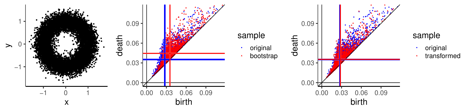
Given a random sample 𝐗n={X1,…,Xn}\mathbf{X}_{n}=\left\{X_{1},...,X_{n}\right\}, it can be shown using elementary arguments that a given bootstrap sample 𝐗n∗\mathbf{X}_{n}^{*} of size nn from the empirical distribution over 𝐗n\mathbf{X}_{n} is expected to contain n⁡(1−(1−1/n)n)≈(1−e−1)​n≈0.632​nn(1-\left({1-1/n}\right)^{n})\approx\left({1-e^{-1}}\right)n\approx 0.632n unique points. As such, 𝐗n∗\mathbf{X}_{n}^{*} behaves similarly to a sample of size 0.632​n0.632n, but is not scaled accordingly within the statistic (βqr,s​(nd​𝐗n∗)−𝔼⁡[βqr,s​(nd​𝐗n∗)|𝐗n])/nd\left({\beta_{q}^{r,s}\left({\sqrt[d]{n}\mathbf{X}_{n}^{*}}\right)-\mathbb{E}\left[{\beta_{q}^{r,s}\left({\sqrt[d]{{n}}\mathbf{X}_{n}^{*}}\right)\big|\mathbf{X}_{n}}\right]}\right)/\sqrt[d]{n}. This discrepancy in scaling introduces a non-negligible asymptotic bias. The effect is illustrated in Figure 1 for the Vietoris-Rips complex.
Refer to caption
Figure 1: Left: The original data set of size n=10,000n=10,000, from which a single standard bootstrap sample is drawn. Middle: Persistence diagrams for both the original and bootstrap samples, along with lines denoting the median birth and death in each diagram. The asymptotic bias discussed in Section 4.1 can be clearly seen. Right: Persistence diagrams after application of a multiplicative correction factor of 1−e−1≈0.795\sqrt{1-e^{-1}}\approx 0.795 to the bootstrap sample. Note that the median birth/death times correspond after transformation.

Furthermore, the standard nonparametric bootstrap results in a fundamentally different point process limit at small scales when compared to the original sample. For the original sample, when 𝐗n\mathbf{X}_{n} is drawn from a distribution with density ff, the shifted and rescaled sample nd​(𝐗n−z)\sqrt[d]{n}\left({\mathbf{X}_{n}-z}\right) approaches a homogeneous Poisson process 𝐏z\mathbf{P}_{z} with intensity f⁡(z)f\left({z}\right). From the preceeding stabilization literature ([38], [31]), this limiting local point process drives the asymptotic sampling distribution of (βqr,s​(nd​𝐗n)−𝔼⁡[βqr,s​(nd​𝐗n)])/nd\left({\beta_{q}^{r,s}\left({\sqrt[d]{n}\mathbf{X}_{n}}\right)-\mathbb{E}\left[{\beta_{q}^{r,s}\left({\sqrt[d]{n}\mathbf{X}_{n}}\right)}\right]}\right)/\sqrt[d]{n}. Considering the large-sample behavior of nd​(𝐗n∗−z)|𝐗n\sqrt[d]{n}\left({\mathbf{X}_{n}^{*}-z}\right)|\mathbf{X}_{n}, the smoothed bootstrap sampling procedure described in Section 2.4 can be shown to reproduce the same local Poisson process 𝐏z\mathbf{P}_{z} asymptotically.

However, the same is not true for the standard bootstrap when repeated points are ignored. In this case, nd​(𝐗n∗−z)|𝐗n\sqrt[d]{n}\left({\mathbf{X}_{n}^{*}-z}\right)|\mathbf{X}_{n} is restricted to the discrete set nd​(𝐗n−z)\sqrt[d]{n}\left({\mathbf{X}_{n}-z}\right), and thus cannot reproduce 𝐏z\mathbf{P}_{z}, whose domain is ℝd\mathbb{R}^{d}. For this case, we describe the resulting point process limit 𝐐z\mathbf{Q}_{z} in two steps. First, a homogenous Poisson process 𝐏z\mathbf{P}_{z} is generated, representing nd​(𝐗n−z)\sqrt[d]{n}\left({\mathbf{X}_{n}-z}\right). Defined conditionally, 𝐐z|𝐏z\mathbf{Q}_{z}|\mathbf{P}_{z} is a random subset of 𝐏z\mathbf{P}_{z} such that ℙ⁡[x∈𝐐z|𝐏z]=1−e−1≈.632\mathbb{P}\left[{x\in\mathbf{Q}_{z}|\mathbf{P}_{z}}\right]=1-e^{-1}\approx.632, considering each point x∈𝐏zx\in\mathbf{P}_{z} independently. We have nd​(𝐗n∗−z)→𝐐z\sqrt[d]{n}\left({\mathbf{X}_{n}^{*}-z}\right)\rightarrow\mathbf{Q}_{z}.

This difference in local behavior, combined with the asymptotic bias effect illustrated earlier, are strong indicators that (βqr,s​(nd​𝐗n∗)−𝔼⁡[βqr,s​(nd​𝐗n∗)]|𝐗n)/nd\left({\beta_{q}^{r,s}\left({\sqrt[d]{n}\mathbf{X}^{*}_{n}}\right)-\mathbb{E}\left[{\beta_{q}^{r,s}\left({\sqrt[d]{n}\mathbf{X}^{*}_{n}}\right)}\right]\big|\mathbf{X}_{n}}\right)/\sqrt[d]{n} and (βqr,s​(nd​𝐗n)−𝔼⁡[βqr,s​(nd​𝐗n)])/nd\\ \left({\beta_{q}^{r,s}\left({\sqrt[d]{n}\mathbf{X}_{n}}\right)-\mathbb{E}\left[{\beta_{q}^{r,s}\left({\sqrt[d]{n}\mathbf{X}_{n}}\right)}\right]}\right)/\sqrt[d]{n} likely do not share a weak limit. A technical treatment is omitted here, and is outlined merely to justify the use of our smoothed bootstrap procedure in place of the standard nonparametric bootstrap. The smoothed bootstrap procedure provides for bootstrap consistency (Corollaries 4.2 and 4.3), and in the following sections we consider only this approach.

4.2 General Conditions for Simplicial Complexes

The results presented in the following sections apply for a range of simplicial complexes constructed over point clouds in ℝd\mathbb{R}^{d}. Here we will explain the specific conditions used, and for which common simplicial complexes they apply. Let KK be a function taking as input S∈𝒳~​(ℝd)S\in\tilde{\mathcal{X}}\left({\mathbb{R}^{d}}\right), giving as output a simplicial complex with vertices in SS. For a given simplex σ\sigma, let the set diameter be diam​(σ)\text{diam}\left({\sigma}\right). We have the following conditions:

  1. (K1)

    For any S∈𝒳~​(ℝd)S\in\tilde{\mathcal{X}}\left({\mathbb{R}^{d}}\right) and z∉Sz\notin S, K⁡(S)⊆K⁡(S∪{z})K\left({S}\right)\subseteq K\left({S\cup\left\{z\right\}}\right). Furthermore, σ∈K⁡(S∪{z})∖K⁡(S)\sigma\in K\left({S\cup\left\{z\right\}}\right)\setminus K\left({S}\right) only if z∈σz\in\sigma.

  2. (K2)

    For any S∈𝒳~​(ℝd)S\in\tilde{\mathcal{X}}\left({\mathbb{R}^{d}}\right) and z∈ℝdz\in\mathbb{R}^{d}, σ∈K⁡(S)\sigma\in K\left({S}\right) only if σ−z∈K⁡(S−z)\sigma-z\in K\left({S-z}\right).

  1. (D1)

    There exists ϕ<∞\phi<\infty such that for any S∈𝒳~​(ℝd)S\in\tilde{\mathcal{X}}\left({\mathbb{R}^{d}}\right), σ∈Kr​(S)\sigma\in K^{r}\left({S}\right) only if diam​(σ)≤ϕ\text{diam}\left({\sigma}\right)\leq\phi.

  2. (D2)

    There exists ϕ<∞\phi<\infty such that for any S∈𝒳~​(ℝd)S\in\tilde{\mathcal{X}}\left({\mathbb{R}^{d}}\right) and z∈ℝdz\in\mathbb{R}^{d}, σ∈K⁡(S∪{z})​△​K​(S)\sigma\in K\left({S\cup\left\{z\right\}}\right)\triangle K\left({S}\right) only if σ⊂Bz​(ϕ)\sigma\subset B_{z}\left({\phi}\right).

  3. (D3)

    There exists an η>0\eta>0 such that for any S∈𝒳~​(ℝd)S\in\tilde{\mathcal{X}}\left({\mathbb{R}^{d}}\right) and x∈Z⁡(K⁡(S))x\in Z\left({K\left({S}\right)}\right), diam​(x)≤η\text{diam}\left({x}\right)\leq\eta only if x∈B⁡(K⁡(S))x\in B\left({K\left({S}\right)}\right).

  4. (D4)

    There exists an m∈ℕm\in\mathbb{N} such that for any k>mk>m and S∈𝒳~​(ℝd)S\in\tilde{\mathcal{X}}\left({\mathbb{R}^{d}}\right), Zk​(K⁡(S))=Bk​(K⁡(S))Z_{k}\left({K\left({S}\right)}\right)=B_{k}\left({K\left({S}\right)}\right).

(K1) means that the addition of a new point will not change the existing complex, only add new simplices. Furthermore, any new simplices gained must contain the added point as a vertex. (K2) gives that the complex is essentially translation invariant. (D1) sets a maximum diameter for any simplex in the complex. (D2) gives that the influence of a new point on the complex is confined to a local region around that point, within a fixed diameter. This condition allows for both the addition and removal of simplices from the complex, but only within the prescribed radius. It can be easily shown that if (D2) holds for ϕ\phi, (D1) holds for 2​ϕ2\phi. Conversely if both (K1) and (D1) hold for ϕ\phi, (D2) also holds for ϕ\phi. Finally, (D3) gives that no small loops can exist with unfilled interiors, and (D4) gives that all Betti numbers are 00 in sufficiently high feature dimensions.

Now, let 𝒦=(Kr)r∈ℝ\mathcal{K}=\left({K^{r}}\right)_{r\in\mathbb{R}} be a function taking as input S∈𝒳~​(ℝd)S\in\tilde{\mathcal{X}}\left({\mathbb{R}^{d}}\right), giving as output a filtration of simplicial complexes with vertices in SS. As a slight abuse, we will often refer to the function 𝒦\mathcal{K} as a filtration of simplicial complexes, even though it is a function defining more than a single filtration, depending on the underlying point cloud. We say that a given condition is satisfied for 𝒦\mathcal{K} if it is satisfied by KrK^{r} for any r∈ℝr\in\mathbb{R}. In the cases of (D1), (D2), and (D3), ϕ\phi and η\eta may depend on rr as increasing functions ϕ:ℝ→[0,∞)\phi\colon\mathbb{R}\rightarrow\left[0,\infty\right) and η:ℝ→[0,∞)\eta\colon\mathbb{R}\rightarrow\left[0,\infty\right).

It can be shown that all of (K1)-(D3) are satisfied for both the Vietoris-Rips and Čech complexes in ℝd\mathbb{R}^{d} using ϕ⁡(r)=η⁡(r)=2​r\phi\left({r}\right)=\eta\left({r}\right)=2r. The same functions apply for the alpha complex in ℝd\mathbb{R}^{d} and its completion 𝒦α∗\mathcal{K}_{\alpha^{*}}, with the notable exception that (K1) is violated. Finally, it is known that (D4) is satisfied by the alpha, Čech, and Delauney complexes in ℝd\mathbb{R}^{d} for m=d−1m=d-1.

While covering a wide class of distance-based simplicial complexes, there are several complexes used in practice that may fail to satisfy any or all of these. For example, the addition of a new point to the Delaunay complex, Gabriel graph, witness complex, or kk-nearest neighbor graph can both add and remove simplices, violating (K1). Furthermore, there is not any limit on the simplex diameter within any of these complexes, violating (D1). Likewise, the addition of a single point can alter simplices at arbitrarily large distances, violating (D2). As a special note, it is common in practice to consider the intersection of the Vietoris-Rips and Delaunay complexes, which unfortunately may violate all the assumptions here. It is unclear if an extension or special consideration could be made to incorporate these complexes.

4.3 Stabilization of Persistent Betti Numbers

To apply the general bootstrap theorem, we first require a technical lemma establishing a locally-determined radius of stabilization for persistent Betti numbers. The result given applies for general classes of simplicial complexes constructed over subsets of ℝd\mathbb{R}^{d}, using the conditions listed previously. Reiterating, 𝒞p,M​(ℝd)\mathcal{C}_{p,M}\left({\mathbb{R}^{d}}\right) is the class of distributions GG on ℝd\mathbb{R}^{d} with densities gg such that ‖g‖p≤M\|g\|_{p}\leq M. We have the following:

Lemma 4.1.

Let F∈𝒞p,M​(ℝd)F\in\mathcal{C}_{p,M}\left({\mathbb{R}^{d}}\right) for some p>2p>2 and M<∞M<\infty, and let 𝒦={Kr}r∈ℝ\mathcal{K}=\left\{K^{r}\right\}_{r\in\mathbb{R}} be a filtration of simplicial complexes satisfying (K2), (D2), and (D3). Then for any r∈ℝr\in\mathbb{R}, s∈ℝs\in\mathbb{R}, and q≥0q\geq 0, βqr,s​(𝒦)\beta_{q}^{r,s}\left({\mathcal{K}}\right) satisfies (S2) for FF.

4.4 Bootstrap Results for Persistence Homology

Here we present the main applied results of this paper. Each is derived from Theorem 2.7 and the stabilization lemma for persistent Betti numbers (Lemma 4.1). For given vectors of birth and death times, r→=(ri)i=1k\vec{r}=\left({r_{i}}\right)_{i=1}^{k} and s→=(si)i=1k\vec{s}=\left({s_{i}}\right)_{i=1}^{k}, let βqr→,s→=(βqri,si)i=1k\beta_{q}^{\vec{r},\vec{s}}=\left({\beta_{q}^{r_{i},s_{i}}}\right)_{i=1}^{k} denote the multivariate function whose components are the persistent Betti numbers evaluated at each pair of birth and death times. For a vector of filtration times r→=(ri)i=1k\vec{r}=\left({r_{i}}\right)_{i=1}^{k}, let χr→\chi^{\vec{r}} denote the function giving the Euler characteristic at each time rir_{i}, with χr→:=(χ⁡(Kri))i=1k\chi^{\vec{r}}:=\left({\chi\left({K^{r_{i}}}\right)}\right)_{i=1}^{k}.

The following apply for F∈𝒫⁡(ℝd)F\in\mathcal{P}\left({\mathbb{R}^{d}}\right) with density ff such that ‖f‖p<∞\|f\|_{p}<\infty for some p>2p>2, as specified. FF and F^n\hat{F}_{n} are such that F^n\hat{F}_{n} has density f^n\hat{f}_{n}, ‖f^n−f‖1→0\|\hat{f}_{n}-f\|_{1}\to 0, and ‖f^n−f‖p→0\|\hat{f}_{n}-f\|_{p}\rightarrow 0 in probability (resp. a.s.a.s.). Let 𝐗n={Xi}i=1n​∼iid​F\mathbf{X}_{n}=\left\{X_{i}\right\}_{i=1}^{n}\overset{\text{iid}}{\sim}F and (mn)n∈ℕ\left({m_{n}}\right)_{n\in\mathbb{N}} such that limn→∞mn=∞\lim_{n\rightarrow\infty}m_{n}=\infty. 𝐗mn∗={Xi∗}i=1mn​∼iid​F^n|𝐗n\mathbf{X}_{m_{n}}^{*}=\left\{X_{i}^{*}\right\}_{i=1}^{m_{n}}\overset{\text{iid}}{\sim}\hat{F}_{n}\big|\mathbf{X}_{n} is a bootstrap sample and GG a multivariate distribution. Recalling the conclusion of Theorem 2.7, for a multivariate statistic ψ→\vec{\psi}:

Statement 4.1.
1n​(ψ→​(nd​𝐗n)−𝔼⁡[ψ→​(nd​𝐗n)])​→𝑑​G\frac{1}{\sqrt{n}}\left({\vec{\psi}\left({\sqrt[d]{n}\mathbf{X}_{n}}\right)-\mathbb{E}\left[{\vec{\psi}\left({\sqrt[d]{n}\mathbf{X}_{n}}\right)}\right]}\right)\overset{d}{\rightarrow}G

if and only if

1mn​(ψ→​(mnd​𝐗mn∗)−𝔼⁡[ψ→​(mnd​𝐗mn∗)|𝐗n])​→𝑑​G​ in probability (resp. a.s.).\frac{1}{\sqrt{{m_{n}}}}\left({\vec{\psi}\left({\sqrt[d]{{m_{n}}}\mathbf{X}_{m_{n}}^{*}}\right)-\mathbb{E}\left[{\vec{\psi}\left({\sqrt[d]{{m_{n}}}\mathbf{X}_{m_{n}}^{*}}\right)\big|\mathbf{X}_{n}}\right]}\right)\overset{d}{\rightarrow}G\text{ in probability (resp. a.s.)}.

For cases with a corresponding central limit theorem, GG is the limiting normal distribution of the original standardized statistic.

Corollary 4.2 (Persistent Betti Numbers).

Let q≥0q\geq 0 and p>2​q+3p>2q+3. Let 𝒦\mathcal{K} be a filtration of simplicial complexes satisfying (K1), (K2), (D1), and (D3). Then for any given r→\vec{r}, s→\vec{s}, Statement 4.1 holds for βqr→,s→\beta_{q}^{\vec{r},\vec{s}}.

Corollary 4.3 (Persistent Betti Numbers - Alt.).

Let q≥0q\geq 0 and p>2​q+5p>2q+5. Let 𝒦\mathcal{K} be a filtration of simplicial complexes satisfying (K2), (D2), and (D3). Then for any given r→\vec{r}, s→\vec{s}, Statement 4.1 holds for βqr→,s→\beta_{q}^{\vec{r},\vec{s}}.

The only differences between the above corollaries are the conditions satisfied by the underlying simplicial complex and the necessary norm bound on the density. The corresponding results for the Betti numbers follow as special cases of Corollaries 4.2 and 4.3, when the given birth and death parameters are equal (βqr→=βqr→,r→\beta^{\vec{r}}_{q}=\beta^{\vec{r},\vec{r}}_{q}). Also, although the statements of Corollaries 4.2 and 4.3 are given in terms of a fixed feature dimension qq, a direct extension exists if q=qiq=q_{i} is allowed to differ for each (ri,si)\left({r_{i},s_{i}}\right). The form as given shows the dependence of the density norm assumption on the chosen feature dimension.

The higher value of pp required in Corollary 4.3 compared to Corollary 4.2 can be explained intuitively based on the assumptions used. For the persistent Betti numbers, the main quantity controlling convergence is the expected number of simplices altered or introduced when a new datapoint is added to the sample. (D2) ensures that these simplices fall within a small ball around the new data point. The stated density norm conditions control the expected number of points, and by extension possible simplices, that can lie within that small ball. Introducing (K1) further controls the number of possible simplices, and allows for a weakening of the necessary norm condition. (K1) requires that, as the sample grows by a single point, any additional simplices must contain the new point as a vertex, and no deletion of simplices is possible. This means that every added simplex has one less “free” vertex, and a weaker norm condition is required for control. The same intuition applies whenever (K1) is assumed.

In the specific case of the alpha complex, both of the above Corollaries 4.2 and 4.3 apply. While the alpha complex does not satisy (K1), it has equal persistent Betti numbers to the Čech complex, which does. Thus, the weaker conditions of Corollary 4.2 are sufficient in this unique case.

Corollary 4.4 (Euler Characteristic).

Let m<∞m<\infty and p>2​m+3p>2m+3. Let 𝒦\mathcal{K} be a filtration of simplicial complexes satisfying (K1), (K2), (D1), (D3), and (D4). Then for any given r→\vec{r}, Statement 4.1 holds for χr→\chi^{\vec{r}}.

Corollary 4.5 (Euler Characteristic - Alt.).

Let m<∞m<\infty and p>2​m+5p>2m+5. Let 𝒦\mathcal{K} be a filtration of simplicial complexes satisfying (K2), (D2), (D3), and (D4). Then for any given r→\vec{r}, Statement 4.1 holds for χr→\chi^{\vec{r}}.

It is suspected that some of the simplicial complex assumptions can be relaxed in the persistent Betti number and Euler characteristic cases, but the extent to which this is possible is still unknown. Specifically, Corollary 4.2 requires a translation-invariant simplicial complex (K2), along with the elimination of small loops via (D3). See Appendix A for altered “BB-bounded persistent Betti number” and “qq-truncated Euler characteristic” problem settings where these issues may be resolved.

To strengthen Corollaries 4.2-4.5 with rates, we require more specific knowledge about the convergence to GG of the original statistic. For persistent Betti numbers in the multivariate setting, general central limit theorems have been shown in [31], but little is known at this time with regards to rates of convergence. Proposition 2.6 does allow for rates of convergence in 2-Wasserstein distance between the bootstrap and true sampling distributions for finite sample sizes, but is phrased in terms of a tail probability for the radius of stabilization. See the proofs of Corollaries 4.2-4.5 for details. For persistent Betti numbers the tail behavior of the radius of stabilization is poorly understood. Owing to these difficulties, we may only conclude consistency of the smoothed bootstrap for the functions considered.

4.5 Bootstrap Results for kk-Nearest Neighbor Graphs

In the following, let 𝒟γ,r0​(C)\mathcal{D}_{\gamma,r_{0}}\left({C}\right) be the class of distributions GG with support on a bounded C⊂ℝdC\subset\mathbb{R}^{d} such that ∫Bx​(r)d​G≥γ​rd\int_{B_{x}\left({r}\right)}\ \text{d}{G}\geq\gamma r^{d} for all r≤r0r\leq r_{0} and x∈Cx\in C.

Corollary 4.6 (Total Edge Length of the kk-Nearest Neighbor Graph).

Let p>2p>2. Furthermore, let F∈𝒟γ,r0​(C)F\in\mathcal{D}_{\gamma,r_{0}}\left({C}\right) and 𝟙{F^n∈𝒟γ,r0(C)}→1\mathbbm{1}\left\{{\hat{F}_{n}\in\mathcal{D}_{\gamma,r_{0}}\left({C}\right)}\right\}\rightarrow 1 in probability (resp. a.s.). Then Statement 4.1 holds for lNN,kl_{\text{NN},k}.

The conditions of Corollary 4.6 are in particular satisfied when CC is known and convex, with ff bounded below on CC by a constant, provided further that ‖f^n−f‖∞→0\|\hat{f}_{n}-f\|_{\infty}\rightarrow 0 in probability (resp. a.s.). We include this final result to demonstrate the utility of stabilization as a general tool for proving bootstrap convergence theorems outside of topological data analysis. The kk-nearest neighbor graph does not fall under the general simplicial complex conditions provided in Section 4.2, thus special treatment is needed to show the required stabilization and moment conditions. Here we rely on previous results from the literature, see [38] for stabilization results and the corresponding central limit theorem.

5 Simulation Study

In this section we present the results of a series of simulations illustrating the finite-sample properties of the smoothed bootstrap applied to persistent Betti numbers βqr,s\beta_{q}^{r,s} of the Vietoris-Rips complex constructed over point sets in ℝd\mathbb{R}^{d}. Precise definitions and an introduction to the properties of these statistics may be found in Section 3. Source code for this section, as well as for the data analysis of Section 6 is available at
github.com/btroycraft/stabilizing_statistics_bootstrap [44].

We investigate the coverage probability of bootstrap confidence intervals on the expected persistent Betti numbers 𝔼⁡[βqr,s​(nd​𝐗n)]\mathbb{E}\left[{\beta_{q}^{r,s}\left({\sqrt[d]{n}\mathbf{X}_{n}}\right)}\right] for a variety of feature dimensions, sample sizes, data generating mechanisms, and bandwidth selectors. Table 1 lists brief descriptions of the data distributions considered. For more detailed explanations, see Appendix D. The results of the simulations are given in Table 2. For the persistent Betti numbers, a single choice of (r,s)\left({r,s}\right) was made for each combination of distribution and feature dimension, chosen to lie within the main body of features in the corresponding persistence diagram. For computational reasons, only feature dimensions q=1q=1 and q=2q=2 are considered.

We consider five data-driven bandwidth selectors. First are the “Hpi.diag” (plug-in), “Hlscv.diag” (least-squares cross-validation), and “Hscv.diag” (smoothed cross-validation) selectors from the ks package in R. Second, we include the adaptive bandwidth selector described in Section 6. While this selector is tailored for the specifics of astronomical data, we include it here for completeness. Each of these four selectors are available for data dimension up to d=6d=6. Last, we consider Silverman’s rule of thumb (see [46]) via “bw.silv” from the kernelboot package in R, which accepts data in any dimension.

For the two cross-validation selectors, note that a bandwidth is not always selected, throwing errors on some datasets. To accommodate the automatic setting of this simulation study, any error-producing data sets were simply rejected for each of these cases.

There is a noticeable drop-off in coverage as the data dimension increases. This is expected, as the kernel density estimator is known to suffer from a “curse of dimensionality”. For distribution F6F_{6}, which exhibits heavy tails, only the adaptive bandwidth selector performed well, because outliers are weighted much less heavily in this case. It is likely that performance will suffer generally in the presence of heavy tailed data when using one of the selectors with common bandwidth.

The coverage proportion is generally smaller than the nominal level of 95%95\%. Therefore, it is recommended to use a larger than desired level, especially for limited sample sizes. In terms of general performance, we recommend any of “Hpi.diag”, “Hlscv.diag”, or “Hscv.diag”. These selectors provide the most consistent coverage, and effectively replicate the nominal 95% level in many cases, especially for the largest sample size n=400n=400. Silverman’s rule performs badly in several cases, and should only be used in the absence of better alternatives.

Label Description
F1F_{1} Rotationally symmetric in ℝ2\mathbb{R}^{2}, finite L8L_{8} norm
F2F_{2} Rotationally symmetric in ℝ2\mathbb{R}^{2}, finite L2L_{2} norm, infinite L8L_{8} norm
F3F_{3} 𝕊1\mathbb{S}^{1} embedded in ℝ2\mathbb{R}^{2}, additive Gaussian noise
F4F_{4} Uniformly distributed over B0​(1)B_{0}\left({1}\right) in ℝ3\mathbb{R}^{3}, additive Gaussian noise
F5F_{5} 5 clusters in ℝ3\mathbb{R}^{3}, additive exponential noise
F6F_{6} 𝕊2\mathbb{S}^{2} embedded in ℝ5\mathbb{R}^{5}, additive Cauchy noise
F7F_{7} Flat figure-8 embedded in ℝ10\mathbb{R}^{10}, additive Gaussian noise
Table 1: Description of densities or distributions considered for the simulation study of Section 5. For the distributions based on manifolds, we first draw uniformly from the manifold, then apply the prescribed additive noise. Detailed explanations of the distributions considered, along with precise definitions are available in Appendix D.
Distr. F1F_{1} F2F_{2} F3F_{3} F4F_{4} F5F_{5} F6F_{6} F7F_{7} F4F_{4} F5F_{5} F6F_{6} F7F_{7}
q=1q=1 q=2q=2
rr 4.94 5.20 3.03 1.92 0.30 1.78 1.28 2.96 0.39 2.71 1.46
ss 5.36 5.60 3.28 2.12 0.31 1.91 1.32 3.04 0.40 2.80 1.47
n=100n=100 0.896 0.965 0.921 0.859 0.954 0.19 0.908 0.705 0.038
0.931 0.959 0.914 0.809 0.941 0.133 0.903 0.604 0.045
0.903 0.97 0.91 0.859 0.927 0.049 0.902 0.363 0.002
0.922 0.898 0.899 0.71 0.725 0.736 0.837 0.048 0.051
0.359 0.931 0.942 0.864 0 0 0.656 0.902 0 0 0.045
n=200n=200 0.908 0.971 0.94 0.898 0.942 0.159 0.878 0.795 0.125
0.92 0.972 0.946 0.891 0.923 0.106 0.872 0.707 0.074
0.888 0.975 0.959 0.906 0.892 0.06 0.908 0.277 0.031
0.888 0.909 0.828 0.783 0.773 0.705 0.673 0.032 0.27
0.299 0.954 0.903 0.899 0 0 0.766 0.882 0 0 0.537
n=300n=300 0.9 0.971 0.926 0.921 0.94 0.183 0.854 0.906 0.225
0.94 0.971 0.938 0.896 0.94 0.087 0.854 0.917 0.072
0.913 0.971 0.94 0.896 0.922 0.054 0.855 0.964 0.074
0.93 0.923 0.864 0.786 0.771 0.735 0.712 0.551 0.575
0.283 0.956 0.925 0.906 0 0 0.835 0.856 0 0 0.508
n=400n=400 0.918 0.961 0.947 0.934 0.96 0.175 0.851 0.883 0.259
0.927 0.951 0.938 0.92 0.955 0.063 0.839 0.88 0.076
0.908 0.976 0.933 0.924 0.939 0.062 0.863 0.958 0.099
0.911 0.922 0.874 0.813 0.825 0.771 0.695 0.952 0.789
0.266 0.961 0.909 0.922 0.114 0 0.891 0.859 0 0 0.584
Table 2: Coverage proportions for 95%95\% smoothed bootstrap confidence intervals on the mean persistent Betti numbers; coverage is estimated using N=1,000N=1,000 independent base samples with B=500B=500 bootstrap samples each. True mean persistent Betti numbers are estimated using a large (N=100,000N=100,000) number of independent samples from the true distribution. For each case, the values from top to bottom: Coverage proportions using “Hpi.diag”, “Hlscv.diag”, “Hscv.diag”, “adaptive”, and “bw.silv” bandwidth selectors, respectively. (see Section 5)

6 Data Analysis

In this section we show how smoothed bootstrap estimation performs on a real dataset. We consider a selection of galaxies from the Sloan Digital Sky Survey [5], chosen from a selection of sky with right ascension values between 100∘100^{\circ} and 270∘270^{\circ} and declination between −7∘-7^{\circ} and 70∘70^{\circ}. Three slices of galaxies were considered, separated by redshift, a measure of radial distance from the solar system. The selections consist of galaxies with red-shift within (0.025,0.026)\left({0.025,0.026}\right), (0.027,0.028)\left({0.027,0.028}\right), and (0.029,0.030)\left({0.029,0.030}\right), respectively. These slices were chosen to investigate the topological properties of the cosmic web across time. In this case, due to the rough homogeneity of the web at large scales, few significant topological deviations are expected.

Subset limits were chosen to maintain computational feasibility and avoid measurement gaps. In an initial cleaning step, each slice was flattened using an area-preserving cylindrical projection and trimmed so that the slices share a common boundary with the same number of galaxies (23742374) per slice. Angular units are converted to distances in Megaparsecs (Mpc) based on the redshift and Hubble’s constant.

The distribution of galaxies in each dataset is modeled by a random sample from some bivariate probability distribution, where the location of each galaxy is drawn independently from the overall distribution. As a part of the model framework, the effect of gravitational interaction manifests via a macroscopic change in the matter distribution, rather than as dependency between individual galaxies.

Following the recommendation of [24], we estimate the density of the matter distribution using the adaptive bandwidth selector described in [8]. This adaptive bandwidth selector was chosen to accommodate for the large variations in density present within astronomy data. The selectors considered in Section 5 do not perform well in this context, often oversmoothing by a large margin. A pilot density estimator was constructed based on the “Hpi.diag” plug-in bandwidth selector and a Gaussian kernel.

Visualizations of the density estimates are provided in Figure 2. Generally, the fit adequately captures the filament structures present in the raw data. Within the persistence diagrams, the mass of features present close to the main diagonal represents small-scale holes between neighboring galaxies, whereas features farther from the diagonal represent the large-scale holes formed by relatively disparate galaxies.

We apply the Vietoris-Rips complex to each of the slices, and calculate a selection of persistent Betti numbers in dimensions q=0q=0 and q=1q=1. The 00-dimensional features summarize cluster and filament structure, whereas the 11-dimensional features describe voids and depressions. The transformed datasets and persistence diagrams in dimension q=1q=1 can be seen in Figure 2. We consider the Betti numbers β0r\beta_{0}^{r} and β1r\beta_{1}^{r}, as well as the persistent Betti numbers β1r,r+1\beta_{1}^{r,r+1} for r=3,…,30r=3,...,30 Mpc. Filtration parameters for the persistent Betti numbers were chosen to lie close to the diagonal r=sr=s, excluding features with a lifetime less than 11 Mpc. We use bootstrap estimation to construct nominal 98%98\% confidence intervals for the population mean values, both pointwise and simultaneous within each regime across r=3,…,30r=3,...,30 Mpc. The number of bootstrap replicates used was B=20,000B=20,000, with results seen in Figure 3.

In feature dimension q=0q=0, the curves show similar behavior across the slices. Consistent with our empirical results, similar Betti curves are expected when the within-filament matter distribution and overall frequency of filaments for each sample are equal. For feature dimension q=1q=1, more variation is present. However, as can be seen from the bootstrap confidence intervals, much of this variation is explained by random fluctuation. For example, while a notable depression around the scale of 88 Mpc exists for the third slice, it is still within the margins of error provided. From this analysis, we do not find significant differences in the topological properties of the three samples over the range of filtration parameters considered. The difference in topological structure seen within each pair of Betti curves is within the margin of error provided by the bootstrap confidence intervals, especially considering the wider simultaneous intervals.

The consistency shown in Section 4.4 for bootstrap estimation applies only for those features within the “body” of topological features, being those occurring at a local scale. Features with large persistence or ones that appear at large diameter are not accounted for in this, as their relative weight is small within the persistent Betti numbers. As such, our analysis does not preclude differences in topology at a large relative scale, describing the largest galactic structures.

Refer to caption
Figure 2: Top row: Transformed point clouds. Middle row: Density estimates using adaptive bandwidth. Bottom row: Persistence diagrams in dimension q=1q=1 for the Vietoris-Rips complex. Columns from left to right: Galaxies with redshifts within (0.025,0.026)\left({0.025,0.026}\right), (0.027,0.028)\left({0.027,0.028}\right), and (0.029,0.030)\left({0.029,0.030}\right), respectively. Axis units are given in Megaparsecs (Mpc).
Figure 3: Betti curves for the Vietoris-Rips complex. Top row: Betti numbers β0r\beta_{0}^{r}. Middle row: Betti numbers β1r\beta_{1}^{r}. Bottom Row: persistent Betti numbers β1r,r+1\beta_{1}^{r,r+1}. Columns correspond with those of Figure 2. Axis units are given in Megaparsecs (Mpc). For each of r=3,…,30r=3,...,30 Mpc, simultaneous bootstrap confidence bands are given in gray, drawn from bootstrap samples of size B=20,000B=20,000. Likewise, pointwise intervals are given in black.

7 Discussion

In this work we have shown the large-sample consistency of multivariate bootstrap estimation for a range of stabilizing statistics. This includes the persistent Betti numbers, the Euler characteristic, and the total edge length of the kk-nearest neighbor graph. However, many open questions still remain.

In Section 4.1 it was argued that the standard nonparametric bootstrap may fail to directly reproduce the correct sampling distribution asymptotically for topological statistics like the persistent Betti numbers. However, there remains the possibility that a corrected version of the standard bootstrap could provide for consistency. As discussed in Section 4.1, standard bootstrap sampling results in a fundamentally different point process limit at small scales. Previous stabilization results primarily consider Poisson and related processes, meaning a full theoretical treatment of the standard bootstrap would likely require reconstructing much of the previous stabilization and central limit theorem results for the alternative limiting process.

The results for the smoothed bootstrap presented here apply only in the multivariate setting, the obvious extension being to stochastic processes. Essential to a process-level result concerning the persistent Betti numbers would be a convenient tail bound for the radius of stabilization, which is yet unavailable. In the case of persistent Betti numbers, there is a strong relationship between the persistent Betti function and an empirical CDF in two dimensions. As such, there is much established theory in that regard which may be applied once stochastic equicontinuity is established.

In practice it is common that data comes not from a density in ℝd\mathbb{R}^{d}, but instead from a manifold. It is suspected that a version of the results in this paper could apply in the manifold setting. However, this requires a bootstrap that adapts to a possibly unknown manifold structure, similar to that found in [28]. Combined with the inherent challenges of working with manifolds, this extension presents many technical hurdles.

Furthermore, in this work we have shown only consistency for bootstrap estimation to a common limiting distribution. The rates of convergence in the 22-Wasserstein distance regarding the persistent Betti numbers rely on the unknown tail properties of the corresponding radius of stabilization. Quantifying these tail properties is a challenging open problem, and seems to be a key step towards an eventual rate calculation, as well as the previously mentioned process-level result.

Finally, there are several statistics of interest, including those based on the Delaunay complex, which do not fit into the specific frameworks provided here. It may be that these statistics may still satisfy Theorem 2.7 in the general case, by techniques others than those provided here.

Acknowledgements

Thank you to the reviewers for their helpful comments and thorough examination of this work.

Benjamin Roycraft was partially supported by the National Science Foundation (NSF), grant number DMS-1148643. Johannes Krebs was partially supported by the German Research Foundation (DFG), grant number KR-4977/2-1. Wolfgang Polonik was partially supported by the National Science Foundation (NSF), grant number DMS-2015575.

Funding for the Sloan Digital Sky Survey IV has been provided by the Alfred P. Sloan Foundation, the U.S. Department of Energy Office of Science, and the Participating Institutions. SDSS-IV acknowledges support and resources from the Center for High-Performance Computing at the University of Utah. The SDSS web site is www.sdss.org.

References

  • [1] [author] Adler, Robert J.R. J., Agami, SaritS. and Pranav, PratyushP. (2017). Modeling and Replicating Statistical Topology and Evidence for CMB Nonhomogeneity. Proc. Natl. Acad. Sci. USA 114 11878–11883. 10.1073/pnas.1706885114 3725115 \endbibitem
  • [2] [author] Aldous, DavidD. and Steele, J. MichaelJ. M. (1992). Asymptotics for Euclidean Minimal Spanning Trees on Random Points. Probab. Theory Related Fields 92 247–258. 10.1007/BF01194923 1161188 \endbibitem
  • [3] [author] Arsuaga, JavierJ., Borrman, TylerT., Cavalcante, RaymondR., Gonzalez, GeorginaG. and Park, CatherineC. (2015). Identification of Copy Number Aberrations in Breast Cancer Subtypes Using Persistence Topology. Microarrays 4 339–369. 10.3390/microarrays4030339 \endbibitem
  • [4] [author] Biscio, Christophe A. N.C. A. N., Chenavier, NicolasN., Hirsch, ChristianC. and Svane, Anne MarieA. M. (2020). Testing Goodness of Fit for Point Processes Via Topological Data Analysis. Electron. J. Stat. 14 1024–1074. 10.1214/20-EJS1683 4067816 \endbibitem
  • [5] [author] Blanton, M. R.M. R., Bershady, M. A.M. A., Abolfathi, B.B., Albareti, F. D.F. D., Allende Prieto, C.C., Almeida, A.A., Alonso-García, J.J., Anders, F.F., Anderson, S. F.S. F., Andrews, B.B. and et al. (2017). Sloan Digital Sky Survey IV: Mapping the Milky Way, Nearby Galaxies, and the Distant Universe. Astronomical Journal 154 28. 10.3847/1538-3881/aa7567 \endbibitem
  • [6] [author] Bobrowski, OmerO. and Mukherjee, SayanS. (2015). The Topology of Probability Distributions on Manifolds. Probab. Theory Related Fields 161 651–686. 10.1007/s00440-014-0556-x 3334278 \endbibitem
  • [7] [author] Boissonnat, Jean-DanielJ.-D., Chazal, FrédéricF. and Yvinec, MarietteM. (2018). Geometric and Topological Inference. Cambridge Texts in Applied Mathematics. Cambridge University Press, Cambridge. 10.1017/9781108297806 3837127 \endbibitem
  • [8] [author] Breiman, LeoL., Meisel, WilliamW. and Purcell, EdwardE. (1977). Variable Kernel Estimates of Multivariate Densities. Technometrics 19 135–144. 10.1080/00401706.1977.10489521 \endbibitem
  • [9] [author] Bubenik, PeterP. (2015). Statistical Topological Data Analysis Using Persistence Landscapes. J. Mach. Learn. Res. 16 77–102. 3317230 \endbibitem
  • [10] [author] Bubenik, PeterP. and Kim, Peter T.P. T. (2007). A Statistical Approach to Persistent Homology. Homology Homotopy Appl. 9 337–362. 2366953 \endbibitem
  • [11] [author] Camara, Pablo G.P. G., Rosenbloom, Daniel I. S.D. I. S., Emmett, Kevin J.K. J., Levine, Arnold J.A. J. and Rabadan, RaulR. (2016). Topological Data Analysis Generates High-Resolution, Genome-wide Maps of Human Recombination. Cell Systems 3 83–94. 10.1016/j.cels.2016.05.008 \endbibitem
  • [12] [author] Chazal, FrédéricF. and Divol, VincentV. (2018). The Density of Expected Persistence Diagrams and Its Kernel Based Estimation. In 34th International Symposium on Computational Geometry. LIPIcs. Leibniz Int. Proc. Inform. 99 Art. No. 26, 15. Schloss Dagstuhl. Leibniz-Zent. Inform., Wadern. 3824270 \endbibitem
  • [13] [author] Chazal, F.F., Fasy, B. T.B. T., Lecci, F.F., Rinaldo, A.A., Singh, A.A. and Wasserman, L.L. (2015). On the Bootstrap for Persistence Diagrams and Landscapes. Modeling and Analysis of Information Systems 20 111–120. 10.18255/1818-1015-2013-6-111-120 \endbibitem
  • [14] [author] Chazal, FrédéricF., Fasy, Brittany TereseB. T., Lecci, FabrizioF., Rinaldo, AlessandroA. and Wasserman, LarryL. (2015). Stochastic Convergence of Persistence Landscapes and Silhouettes. J. Comput. Geom. 6 140–161. 3323391 \endbibitem
  • [15] [author] Chazal, FrédéricF. and Michel, BertrandB. (2017). An Introduction to Topological Data Analysis: Fundamental and Practical Aspects for Data Scientists. \endbibitem
  • [16] [author] Chen, Yen-ChiY.-C., Wang, DarenD., Rinaldo, AlessandroA. and Wasserman, LarryL. (2015). Statistical Analysis of Persistence Intensity Functions. \endbibitem
  • [17] [author] Chung, Yu-MinY.-M. and Lawson, AustinA. (2019). Persistence Curves: A Canonical Framework for Summarizing Persistence Diagrams. \endbibitem
  • [18] [author] Crawford, LorinL., Monod, AntheaA., Chen, Andrew X.A. X., Mukherjee, SayanS. and Rabadán, RaúlR. (2019). Predicting Clinical Outcomes in Glioblastoma: An Application of Topological and Functional Data Analysis. Journal of the American Statistical Association 1–12. 10.1080/01621459.2019.1671198 \endbibitem
  • [19] [author] Devroye, LucL., Györfi, LászlóL., Lugosi, GáborG. and Walk, HarroH. (2017). On the Measure of Voronoi Cells. J. Appl. Probab. 54 394–408. 10.1017/jpr.2017.7 3668473 \endbibitem
  • [20] [author] Devroye, L. P.L. P. and Wagner, T. J.T. J. (1979). The L1L_{1} Convergence of Kernel Density Estimates. Ann. Statist. 7 1136–1139. 536515 \endbibitem
  • [21] [author] DeWoskin, D.D., Climent, J.J., Cruz-White, I.I., Vazquez, M.M., Park, C.C. and Arsuaga, J.J. (2010). Applications of Computational Homology to the Analysis of Treatment Response in Breast Cancer Patients. Topology Appl. 157 157–164. 10.1016/j.topol.2009.04.036 2556091 \endbibitem
  • [22] [author] Edelsbrunner, Letscher and Zomorodian (2002). Topological Persistence and Simplification. Discrete & Computational Geometry 28 511–533. 10.1007/s00454-002-2885-2 \endbibitem
  • [23] [author] Fasy, Brittany TereseB. T., Lecci, FabrizioF., Rinaldo, AlessandroA., Wasserman, LarryL., Balakrishnan, SivaramanS. and Singh, AartiA. (2014). Confidence Sets for Persistence Diagrams. Ann. Statist. 42 2301–2339. 10.1214/14-AOS1252 3269981 \endbibitem
  • [24] [author] Ferdosi, B. J.B. J., Buddelmeijer, H.H., Trager, S. C.S. C., Wilkinson, M. H. F.M. H. F. and Roerdink, J. B. T. M.J. B. T. M. (2011). Comparison of Density Estimation Methods for Astronomical Datasets. Astronomy & Astrophysics 531 A114. 10.1051/0004-6361/201116878 \endbibitem
  • [25] [author] Folland, Gerald B.G. B. (1999). Real Analysis: Modern Techniques and Applications. Wiley. \endbibitem
  • [26] [author] Hansen, Bruce E.B. E. (2008). Uniform Convergence Rates for Kernel Estimation with Dependent Data. Econometric Theory 24 726–748. 10.1017/S0266466608080304 2409261 \endbibitem
  • [27] [author] Hiraoka, YasuakiY., Shirai, TomoyukiT. and Trinh, Khanh DuyK. D. (2018). Limit Theorems for Persistence Diagrams. Ann. Appl. Probab. 28 2740–2780. 10.1214/17-AAP1371 3847972 \endbibitem
  • [28] [author] Kim, JisuJ., Shin, JaehyeokJ., Rinaldo, AlessandroA. and Wasserman, LarryL. (2018). Uniform Convergence Rate of the Kernel Density Estimator Adaptive to Intrinsic Volume Dimension. \endbibitem
  • [29] [author] Kramar, M.M., Goullet, A.A., Kondic, L.L. and Mischaikow, K.K. (2013). Persistence of Force Networks in Compressed Granular Media. Physical Review E 87. 10.1103/physreve.87.042207 \endbibitem
  • [30] [author] Kramár, MiroslavM., Levanger, RachelR., Tithof, JeffreyJ., Suri, BalachandraB., Xu, MuM., Paul, MarkM., Schatz, Michael F.M. F. and Mischaikow, KonstantinK. (2016). Analysis of Kolmogorov Flow and Rayleigh–bénard Convection Using Persistent Homology. Physica D: Nonlinear Phenomena 334 82–98. 10.1016/j.physd.2016.02.003 \endbibitem
  • [31] [author] Krebs, Johannes T. N.J. T. N. and Polonik, WolfgangW. (2019). On the Asymptotic Normality of Persistent Betti Numbers. \endbibitem
  • [32] [author] Lachièze-Rey, RaphaëlR., Schulte, MatthiasM. and Yukich, J. E.J. E. (2019). Normal Approximation for Stabilizing Functionals. The Annals of Applied Probability 29. 10.1214/18-aap1405 \endbibitem
  • [33] [author] Lachièze-Rey, RaphaëlR., Peccati, GiovanniG. and Yang, XiaochuanX. (2020). Quantitative Two-scale Stabilization on the Poisson Space. \endbibitem
  • [34] [author] Last, GünterG., Peccati, GiovanniG. and Schulte, MatthiasM. (2015). Normal Approximation on Poisson Spaces: Mehler’s Formula, Second Order Poincaré Inequalities and Stabilization. Probability Theory and Related Fields 165 667–723. 10.1007/s00440-015-0643-7 \endbibitem
  • [35] [author] Latała, RafałR. (1997). Estimation of Moments of Sums of Independent Real Random Variables. Ann. Probab. 25 1502–1513. 10.1214/aop/1024404522 1457628 \endbibitem
  • [36] [author] Owada, TakashiT. (2018). Limit Theorems for Betti Numbers of Extreme Sample Clouds with Application to Persistence Barcodes. Ann. Appl. Probab. 28 2814–2854. 10.1214/17-AAP1375 3847974 \endbibitem
  • [37] [author] Owada, TakashiT. and Adler, Robert J.R. J. (2017). Limit Theorems for Point Processes under Geometric Constraints (and Topological Crackle). Ann. Probab. 45 2004–2055. 10.1214/16-AOP1106 3650420 \endbibitem
  • [38] [author] Penrose, Mathew D.M. D. and Yukich, J. E.J. E. (2001). Central Limit Theorems for Some Graphs in Computational Geometry. Ann. Appl. Probab. 11 1005–1041. 10.1214/aoap/1015345393 1878288 \endbibitem
  • [39] [author] Penrose, Mathew D.M. D. and Yukich, J. E.J. E. (2003). Weak Laws of Large Numbers in Geometric Probability. Ann. Appl. Probab. 13 277–303. 10.1214/aoap/1042765669 1952000 \endbibitem
  • [40] [author] Politis, Dimitris N.D. N., Romano, Joseph P.J. P. and Wolf, MichaelM. (1999). Subsampling. Springer Series in Statistics. Springer-Verlag, New York. 10.1007/978-1-4612-1554-7 1707286 \endbibitem
  • [41] [author] Pranav, PratyushP., Adler, Robert J.R. J., Buchert, ThomasT., Edelsbrunner, HerbertH., Jones, Bernard J. T.B. J. T., Schwartzman, ArminA., Wagner, HubertH. and van de Weygaert, RienR. (2019). Unexpected Topology of the Temperature Fluctuations in the Cosmic Microwave Background. Astronomy & Astrophysics 627 A163. 10.1051/0004-6361/201834916 \endbibitem
  • [42] [author] Pranav, PratyushP., Edelsbrunner, HerbertH., van de Weygaert, RienR., Vegter, GertG., Kerber, MichaelM., Jones, Bernard J. T.B. J. T. and Wintraecken, MathijsM. (2016). The Topology of the Cosmic Web in Terms of Persistent Betti Numbers. Monthly Notices of the Royal Astronomical Society 465 4281–4310. 10.1093/mnras/stw2862 \endbibitem
  • [43] [author] Pranav, PratyushP., van de Weygaert, RienR., Vegter, GertG., Jones, Bernard J TB. J. T., Adler, Robert JR. J., Feldbrugge, JobJ., Park, ChangbomC., Buchert, ThomasT. and Kerber, MichaelM. (2019). Topology and Geometry of Gaussian Random Fields I: On Betti Numbers, Euler Characteristic, and Minkowski Functionals. Monthly Notices of the Royal Astronomical Society 485 4167–4208. 10.1093/mnras/stz541 \endbibitem
  • [44] [author] Roycraft, BenjaminB. (2021). github.com/btroycraft/stabilizing_statistics_bootstrap. 10.5281/ZENODO.4627098 \endbibitem
  • [45] [author] Roycraft, BenjaminB., Krebs, JohannesJ. and Polonik, WolfgangW. (2021). Supplement to ”Bootstrapping Persistent Betti Numbers and Other Stabilizing Statistics”. \endbibitem
  • [46] [author] Silverman, B. W.B. W. (1986). Density Estimation for Statistics and Data Analysis. Monographs on Statistics and Applied Probability. Chapman & Hall, London. 10.1007/978-1-4899-3324-9 848134 \endbibitem
  • [47] [author] Singh, ShashankS. and Póczos, BarnabásB. (2016). Analysis of k-Nearest Neighbor Distances with Application to Entropy Estimation. \endbibitem
  • [48] [author] Trinh, Khanh DuyK. D. (2019). On Central Limit Theorems in Stochastic Geometry for Add-one Cost Stabilizing Functionals. Electron. Commun. Probab. 24 Paper No. 76, 15. 10.1214/19-ecp279 4049088 \endbibitem
  • [49] [author] Turner, KatharineK., Mukherjee, SayanS. and Boyer, Doug M.D. M. (2014). Persistent Homology Transform for Modeling Shapes and Surfaces. Inf. Inference 3 310–344. 10.1093/imaiai/iau011 3311455 \endbibitem
  • [50] [author] Ulmer, M.M., Ziegelmeier, LoriL. and Topaz, Chad M.C. M. (2019). A Topological Approach to Selecting Models of Biological Experiments. PLOS ONE 14 1-18. 10.1371/journal.pone.0213679 \endbibitem
  • [51] [author] Wasserman, LarryL. (2018). Topological Data Analysis. Annu. Rev. Stat. Appl. 5 501–535. 10.1146/annurev-statistics-031017-100045 3774757 \endbibitem
  • [52] [author] Xia, KelinK., Feng, XinX., Tong, YiyingY. and Wei, Guo WeiG. W. (2014). Persistent Homology for the Quantitative Prediction of Fullerene Stability. Journal of Computational Chemistry 36 408–422. 10.1002/jcc.23816 \endbibitem
  • [53] [author] Yogeshwaran, D.D. and Adler, Robert J.R. J. (2015). On the Topology of Random Complexes Built Over Stationary Point Processes. Ann. Appl. Probab. 25 3338–3380. 10.1214/14-AAP1075 3404638 \endbibitem
  • [54] [author] Yogeshwaran, D.D., Subag, EliranE. and Adler, Robert J.R. J. (2017). Random Geometric Complexes in the Thermodynamic Regime. Probab. Theory Related Fields 167 107–142. 10.1007/s00440-015-0678-9 3602843 \endbibitem
  • [55] [author] Zomorodian, AfraA. and Carlsson, GunnarG. (2005). Computing Persistent Homology. Discrete Comput. Geom. 33 249–274. 10.1007/s00454-004-1146-y 2121296 \endbibitem

Appendix A Altered Problem Settings

A.1 BB-Bounded Persistent Betti Numbers

To effectively quantify the radius of stabilization for persistent Betti numbers, it is necessary to place controls on the size of possible cycles within a simplicial complex. Large loops extend the influence of a single point beyond the local region, and complicate statistical analysis. As such, we present the following definitions which eliminate any large loops. Note that the statistics of this appendix are presented for their convenient theoretical properties, not their practical significance. Let S∈𝒳~​(ℝd)S\in\tilde{\mathcal{X}}\left({\mathbb{R}^{d}}\right) and K=K⁡(S)K=K\left({S}\right) be a simplicial complex with vertices in SS. For a given chain of simplices ∑i=1mσi∈C⁡(K⁡(S))\sum_{i=1}^{m}\sigma_{i}\in C\left({K\left({S}\right)}\right), we have the diameter given by diam​(∑i=1mσi):=diam​(⋃i=1mσi)\text{diam}\left({\sum_{i=1}^{m}\sigma_{i}}\right):=\text{diam}\left({\bigcup_{i=1}^{m}\sigma_{i}}\right). Let the space of BB-bounded cycles of the complex KK be the vector space, denoted by Zq,B​(K)Z_{q,B}\left({K}\right), spanned by cycles in KK with diameter no larger than BB. We have Zq,B(K):=span{x∈Zq(K) s.t. diam(x)≤B}Z_{q,B}\left({K}\right):=\text{span}\left\{x\in Z_{q}\left({K}\right)\text{ s.t. }\text{diam}\left({x}\right)\leq B\right\}. Likewise let the space of BB-bounded boundaries be Bq,B(K):=span{x∈Bq(K) s.t. diam(x)≤B}B_{q,B}\left({K}\right):=\text{span}\left\{x\in B_{q}\left({K}\right)\text{ s.t. }\text{diam}\left({x}\right)\leq B\right\}.

The definitions presented here are directly inspired by a previous concept under the name “MM-bounded persistence” found in [4], and may be viewed as a generalization thereof. In this previous work, it was shown that a diameter bound of this type is sufficient for establishing functional central limit theorems for persistent Betti numbers, and thus an extension is desireable. The original definition given in [4] is based on a correspondence between loops and connected components in the complement space, and does not apply to arbitrary simplicial complexes and feature dimensions.

The change in naming effected here is not meant to drawn a distinction between the two definitions, but purely to avoid overloading symbols within this paper. MM is used in this work to denote an upper bound for a density norm.

The BB-bounded spaces obey many of the same properties as their original counterparts. We have Bq,M​(K)⊆Zq,M​(K)B_{q,M}\left({K}\right)\subseteq Z_{q,M}\left({K}\right). Thus we can define the BB-bounded homology spaces as Hq,B​(K)=Zq,B​(K)/Bq,B​(K)H_{q,B}\left({K}\right)=Z_{q,B}\left({K}\right)/B_{q,B}\left({K}\right). It should be noted that these definitions allow for chains of unbounded diameter, so long as there exists a decomposition into a sum of bounded chains. Furthermore, for Bq,B​(K)B_{q,B}\left({K}\right), the diameter control is on the chains x∈Bq​(K)x\in B_{q}\left({K}\right), not on a corresponding y∈Cq+1​(K)y\in C_{q+1}\left({K}\right) with x=∂yx=\partial y. It is possible to have a chain with arbitrarily high diameter, whose boundary has diameter less than BB.

We next define the analog of Betti numbers and persistent Betti numbers over a filtration of simplicial complexes in the bounded context. Given a filtration 𝒦={Kr}r∈ℝ\mathcal{K}=\left\{K^{r}\right\}_{r\in\mathbb{R}}, we have BB-bounded analogs for the Betti numbers, persistent homology spaces, and persistent Betti numbers given by

βq,Br​(𝒦)\displaystyle\beta_{q,B}^{r}\left({\mathcal{K}}\right) :=dim(Hq,B​(Kr))\displaystyle:=\dim\left({H_{q,B}\left({K^{r}}\right)}\right) (A.1)
=dim(Zq,B​(Kr))−dim(Bq,B​(Kr))\displaystyle=\dim\left({Z_{q,B}\left({K^{r}}\right)}\right)-\dim\left({B_{q,B}\left({K^{r}}\right)}\right) (A.2)
Hq,Br,s​(𝒦)\displaystyle H_{q,B}^{r,s}\left({\mathcal{K}}\right) :=Zq,B​(Kr)Zq,B​(Kr)∩Bq,B​(Ks)\displaystyle:=\frac{Z_{q,B}\left({K^{r}}\right)}{Z_{q,B}\left({K^{r}}\right)\cap B_{q,B}\left({K^{s}}\right)} (A.3)
βq,Br,s​(𝒦)\displaystyle\beta_{q,B}^{r,s}\left({\mathcal{K}}\right) :=dim(Hq,Br,s​(𝒦))\displaystyle:=\dim\left({H_{q,B}^{r,s}\left({\mathcal{K}}\right)}\right) (A.4)
=dim(Zq,B​(Kr))−dim(Zq,B​(Kr)∩Bq,B​(Ks)).\displaystyle=\dim\left({Z_{q,B}\left({K^{r}}\right)}\right)-\dim\left({Z_{q,B}\left({K^{r}}\right)\cap B_{q,B}\left({K^{s}}\right)}\right). (A.5)

Unfortunately, no direct analog of the Geometric Lemma 3.1 exists for BB-bounded persistent Betti numbers. The addition of a positive simplex can add more than one dimension to Zq,BZ_{q,B}. Consider ZqZ_{q} consisting of a single cycle with diameter above BB but below 2​B2B, meaning Zq,B={0}Z_{q,B}=\left\{0\right\} initially. Now let the loop be split in two by a new simplex σ\sigma. Each piece may now be of diameter less than BB, unlike the original. In this way a single simplex can increase the dimension of Zq,BZ_{q,B} by two or more. The same is true for the negative simplices. Consider the same setup, but now extend each simplex towards a distant point xx in a cone. In this case we have Zq,B=Bq,B={0}Z_{q,B}=B_{q,B}=\left\{0\right\} initially. The inclusion of the simplex σ∪{x}\sigma\cup\left\{x\right\} will split the boundary space just as before into two bounded pieces.

Thus it becomes clear that we must utilize slightly different techniques when considering BB-bounded persistence. We have the following inequality, the analog of the Geometric Lemma for BB-bounded persistent Betti numbers.

Lemma A.1.

Let 𝒥={Jr}r∈ℝ\mathcal{J}=\left\{J^{r}\right\}_{r\in\mathbb{R}} and 𝒦={Kr}r∈ℝ\mathcal{K}=\left\{K^{r}\right\}_{r\in\mathbb{R}} be filtrations of simplicial complexes with Jr⊆KrJ^{r}\subseteq K^{r} for all r∈ℝr\in\mathbb{R}. Then

|βq,Br,s​(𝒦)−βq,Br,s​(𝒥)|≤\displaystyle\left|{\beta_{q,B}^{r,s}\left({\mathcal{K}}\right)-\beta_{q,B}^{r,s}\left({\mathcal{J}}\right)}\right|\leq\ max⁡{dim(Zq,B​(Kr)Zq,B​(Jr)),dim(Bq,B​(Ks)Bq,B​(Js))}\displaystyle\max\left\{\dim\left({\frac{Z_{q,B}\left({K^{r}}\right)}{Z_{q,B}\left({J^{r}}\right)}}\right),\dim\left({\frac{B_{q,B}\left({K^{s}}\right)}{B_{q,B}\left({J^{s}}\right)}}\right)\right\} (A.6)
≤\displaystyle\leq\ dim(Zq,B​(Kr)Zq,B​(Jr))+dim(Bq,B​(Ks)Bq,B​(Js)).\displaystyle\dim\left({\frac{Z_{q,B}\left({K^{r}}\right)}{Z_{q,B}\left({J^{r}}\right)}}\right)+\dim\left({\frac{B_{q,B}\left({K^{s}}\right)}{B_{q,B}\left({J^{s}}\right)}}\right). (A.7)
Proof.
|βq,Br,s​(𝒦)−βq,Br,s​(𝒥)|\displaystyle\left|{\beta_{q,B}^{r,s}\left({\mathcal{K}}\right)-\beta_{q,B}^{r,s}\left({\mathcal{J}}\right)}\right|
=\displaystyle=\ |dim(Zq,B​(Kr)Zq,B​(Kr)∩Bq,B​(Ks))−dim(Zq,B​(Jr)Zq,B​(Jr)∩Bq,B​(Js))|\displaystyle\left|{\dim\left({\frac{Z_{q,B}\left({K^{r}}\right)}{Z_{q,B}\left({K^{r}}\right)\cap B_{q,B}\left({K^{s}}\right)}}\right)-\dim\left({\frac{Z_{q,B}\left({J^{r}}\right)}{Z_{q,B}\left({J^{r}}\right)\cap B_{q,B}\left({J^{s}}\right)}}\right)}\right|
=\displaystyle=\ |dim(Zq,B​(Kr)+Bq,B​(Kr)Zq,B​(Jr)+Bq,B​(Kr))−dim(Zq,B​(Jr)∩Bq,B​(Ks)Zq,B​(Jr)∩Bq,B​(Js))|\displaystyle\left|{\dim\left({\frac{Z_{q,B}\left({K^{r}}\right)+B_{q,B}\left({K^{r}}\right)}{Z_{q,B}\left({J^{r}}\right)+B_{q,B}\left({K^{r}}\right)}}\right)-\dim\left({\frac{Z_{q,B}\left({J^{r}}\right)\cap B_{q,B}\left({K^{s}}\right)}{Z_{q,B}\left({J^{r}}\right)\cap B_{q,B}\left({J^{s}}\right)}}\right)}\right|
≤\displaystyle\leq\ max⁡{dim(Zq,B​(Kr)+Bq,B​(Kr)Zq,B​(Jr)+Bq,B​(Kr)),dim(Zq,B​(Jr)∩Bq,B​(Ks)Zq,B​(Jr)∩Bq,B​(Js))}\displaystyle\max\left\{\dim\left({\frac{Z_{q,B}\left({K^{r}}\right)+B_{q,B}\left({K^{r}}\right)}{Z_{q,B}\left({J^{r}}\right)+B_{q,B}\left({K^{r}}\right)}}\right),\dim\left({\frac{Z_{q,B}\left({J^{r}}\right)\cap B_{q,B}\left({K^{s}}\right)}{Z_{q,B}\left({J^{r}}\right)\cap B_{q,B}\left({J^{s}}\right)}}\right)\right\}
≤\displaystyle\leq\ max⁡{dim(Zq,B​(Kr)Zq,B​(Jr)),dim(Bq,B​(Ks)Bq,B​(Js))}\displaystyle\max\left\{\dim\left({\frac{Z_{q,B}\left({K^{r}}\right)}{Z_{q,B}\left({J^{r}}\right)}}\right),\dim\left({\frac{B_{q,B}\left({K^{s}}\right)}{B_{q,B}\left({J^{s}}\right)}}\right)\right\}
≤\displaystyle\leq\ dim(Zq,B​(Kr)Zq,B​(Jr))+dim(Bq,B​(Ks)Bq,B​(Js)).\displaystyle\dim\left({\frac{Z_{q,B}\left({K^{r}}\right)}{Z_{q,B}\left({J^{r}}\right)}}\right)+\dim\left({\frac{B_{q,B}\left({K^{s}}\right)}{B_{q,B}\left({J^{s}}\right)}}\right).

∎

We make a note here about the difference between Lemma A.1 and the Geometric Lemma 3.1. While drawn from the same fundamental inequality, in the persistent Betti number case, we reduce to counting the simplices that are added when moving from one complex to the other. This reduction cannot be made in the BB-bounded case, and we must count the number of additional linearly independent loops and boundaries. Different combinatorial techniques will be needed when applying each lemma, as can be seen in the proofs of Corollaries 4.2, 4.3, and A.6.

A.2 Stabilization Results

We define the qq-truncated Euler characteristics as

χq​(K):=∑k=0q(−1)k​#​{Kk}.\chi_{q}\left({K}\right):=\sum\limits_{k=0}^{q}\left({-1}\right)^{k}\#\left\{K_{k}\right\}. (A.8)

We have the following stabilization lemmas for BB-bounded persistent Betti numbers and qq-truncated Euler characteristics. Since in both Lemmas A.2 and A.3 the radius of stabilization is a deterministic constant, (S2) is satisfied for any distribution GG. The same is true in the following results for the truncated Euler characteristics.

Lemma A.2.

Let 𝒦\mathcal{K} satisfy (K1). Then for any B≥0B\geq 0, r∈ℝr\in\mathbb{R}, s∈ℝs\in\mathbb{R}, q∈ℕ0q\in\mathbb{N}_{0}, and z∈ℝdz\in\mathbb{R}^{d}, ρz=2​B\rho_{z}=2B is a locally determined radius of stabilization for βq,Br,s​(𝒦)\beta_{q,B}^{r,s}\left({\mathcal{K}}\right) centered at zz.

Proof.

Let a≥2​Ba\geq 2B and S∈𝒳⁡(ℝd)S\in\mathcal{X}\left({\mathbb{R}^{d}}\right). We decompose Zq,B​(Kr​((S∩Bz​(a))∪{z}))Z_{q,B}\left({K^{r}\left({\left({S\cap B_{z}\left({a}\right)}\right)\cup\left\{z\right\}}\right)}\right) into three spaces. Let UzU_{z} be spanned by the generators of Zq,B​(Kr​((S∩Bz​(a))∪{z}))Z_{q,B}\left({K^{r}\left({\left({S\cap B_{z}\left({a}\right)}\right)\cup\left\{z\right\}}\right)}\right) with zz as a vertex. Let UaU_{a} be spanned by the generators with vertices within Bz​(a)∖Bz​(2​B)B_{z}\left({a}\right)\setminus B_{z}\left({2B}\right). Finally, let U∗U_{*} be spanned by the generators without zz as a vertex and with no vertices within Bz​(a)∖Bz​(2​B)B_{z}\left({a}\right)\setminus B_{z}\left({2B}\right). Since the generators of Zq,B​(Kr​((S∩Bz​(a))∪{z}))Z_{q,B}\left({K^{r}\left({\left({S\cap B_{z}\left({a}\right)}\right)\cup\left\{z\right\}}\right)}\right) have diameter at most BB, there are no generating cycles with vertices both at zz and in Bz​(a)∖Bz​(2​B)B_{z}\left({a}\right)\setminus B_{z}\left({2B}\right).

By (K1) we have Zq,B​(Kr​((S∩Bz​(a))∪{z}))=Uz+Ua+U∗Z_{q,B}\left({K^{r}\left({\left({S\cap B_{z}\left({a}\right)}\right)\cup\left\{z\right\}}\right)}\right)=U_{z}+U_{a}+U_{*}, Zq,B​(Kr​(S∩Bz​(a)))=Ua+U∗Z_{q,B}\left({K^{r}\left({S\cap B_{z}\left({a}\right)}\right)}\right)=U_{a}+U_{*}, Zq,B​(Kr​((S∩Bz​(2​B))∪{z}))=Uz+U∗Z_{q,B}\left({K^{r}\left({\left({S\cap B_{z}\left({2B}\right)}\right)\cup\left\{z\right\}}\right)}\right)=U_{z}+U_{*}, and Zq,B​(Kr​(S∩Bz​(2​B)))=U∗Z_{q,B}\left({K^{r}\left({S\cap B_{z}\left({2B}\right)}\right)}\right)=U_{*}.

Now for any cycle within UzU_{z}, the associated vertex set must lie within Bz​(B)B_{z}\left({B}\right). Likewise, for any cycle in UaU_{a}, the associated vertex set must lie within Bz​(a)∖Bz​(B)B_{z}\left({a}\right)\setminus B_{z}\left({B}\right). These vertex sets cannot intersect, thus Uz∩Ua={0}U_{z}\cap U_{a}=\left\{0\right\}.

Now, consider any vector spaces XX, YY, and ZZ such that X∩Y={0}X\cap Y=\left\{0\right\}. Because X∩Y∩ZX\cap Y\cap Z is a subspace of X∩YX\cap Y, it is also the trivial space {0}\left\{0\right\}. We have

dim(X+Y+Z)−dim(Y+Z)\displaystyle\dim\left({X+Y+Z}\right)-\dim\left({Y+Z}\right) (A.9)
=\displaystyle=\ dim(X)−dim(X∩Y)−dim(X∩Z)+dim(X∩Y∩Z)\displaystyle\dim\left({X}\right)-\dim\left({X\cap Y}\right)-\dim\left({X\cap Z}\right)+\dim\left({X\cap Y\cap Z}\right)
=\displaystyle=\ dim(X)−dim(X∩Z)\displaystyle\dim\left({X}\right)-\dim\left({X\cap Z}\right)
=\displaystyle=\ dim(X+Z)−dim(Z).\displaystyle\dim\left({X+Z}\right)-\dim\left({Z}\right). (A.10)

We use this result in each of the following. We have

dim(Zq,B​(Kr​((S∩Bz​(a))∪{z})))−dim(Zq,B​(Kr​(S∩Bz​(a))))\displaystyle\dim\left({Z_{q,B}\left({K^{r}\left({\left({S\cap B_{z}\left({a}\right)}\right)\cup\left\{z\right\}}\right)}\right)}\right)-\dim\left({Z_{q,B}\left({K^{r}\left({S\cap B_{z}\left({a}\right)}\right)}\right)}\right) (A.11)
=\displaystyle=\ dim(Uz+Ua+U∗)−dim(Ua+U∗)\displaystyle\dim\left({U_{z}+U_{a}+U_{*}}\right)-\dim\left({U_{a}+U_{*}}\right)
=\displaystyle=\ dim(Uz+U∗)−dim(U∗)\displaystyle\dim\left({U_{z}+U_{*}}\right)-\dim\left({U_{*}}\right)
=\displaystyle=\ dim(Zq,B​(Kr​((S∩Bz​(2​B))∪{z})))−dim(Zq,B​(Kr​(S∩B0​(2​B)))).\displaystyle\dim\left({Z_{q,B}\left({K^{r}\left({\left({S\cap B_{z}\left({2B}\right)}\right)\cup\left\{z\right\}}\right)}\right)}\right)-\dim\left({Z_{q,B}\left({K^{r}\left({S\cap B_{0}\left({2B}\right)}\right)}\right)}\right). (A.12)

A similar result holds for the boundaries. Let VzV_{z}, VaV_{a}, and V∗V_{*} be defined similarly to UzU_{z}, UaU_{a}, and U∗U_{*}, respectively, instead using the generators of Bq,B​(Ks​((S∩Bz​(a))∪{z}))B_{q,B}\left({K^{s}\left({\left({S\cap B_{z}\left({a}\right)}\right)\cup\left\{z\right\}}\right)}\right). Similarly Bq,B​(Ks​((S∩Bz​(a))∪{z}))=Vz+Va+V∗B_{q,B}\left({K^{s}\left({\left({S\cap B_{z}\left({a}\right)}\right)\cup\left\{z\right\}}\right)}\right)=V_{z}+V_{a}+V_{*}, Bq,B​(Ks​((S∩Bz​(2​B))∪{z}))=Vz+V∗B_{q,B}\left({K^{s}\left({\left({S\cap B_{z}\left({2B}\right)}\right)\cup\left\{z\right\}}\right)}\right)=V_{z}+V_{*}, and we conclude Vz∩Va={0}V_{z}\cap V_{a}=\left\{0\right\}. Furthermore, we have Uz∩Va=Vz∩Ua={0}U_{z}\cap V_{a}=V_{z}\cap U_{a}=\left\{0\right\} by similar vertex-based arguments. Then (Uz+Vz)∩(Ua+Va)={0}\left({U_{z}+V_{z}}\right)\cap\left({U_{a}+V_{a}}\right)=\left\{0\right\}. We have

dim(Zq,B​(Kr​((S∩Bz​(a))∪{z}))∩Bq,B​(Ks​((S∩Bz​(a))∪{z})))\displaystyle\dim\left({Z_{q,B}\left({K^{r}\left({\left({S\cap B_{z}\left({a}\right)}\right)\cup\left\{z\right\}}\right)}\right)\cap B_{q,B}\left({K^{s}\left({\left({S\cap B_{z}\left({a}\right)}\right)\cup\left\{z\right\}}\right)}\right)}\right)
−dim(Zq,B(Kr(S∩Bz(a)))∩Bq,B(Ks(S∩Bz(a))))\displaystyle-\dim\left({Z_{q,B}\left({K^{r}\left({S\cap B_{z}\left({a}\right)}\right)}\right)\cap B_{q,B}\left({K^{s}\left({S\cap B_{z}\left({a}\right)}\right)}\right)}\right)
=\displaystyle=\ dim((Uz+Ua+U∗)∩(Vz+Va+V∗))\displaystyle\dim\left({\left({U_{z}+U_{a}+U_{*}}\right)\cap\left({V_{z}+V_{a}+V_{*}}\right)}\right)
−dim((Ua+U∗)∩(Va+V∗))\displaystyle-\dim\left({\left({U_{a}+U_{*}}\right)\cap\left({V_{a}+V_{*}}\right)}\right)
=\displaystyle=\ dim(Uz+Ua+U∗)+dim(Vz+Va+V∗)−dim(Uz+Ua+U∗+Vz+Va+V∗)\displaystyle\dim\left({U_{z}+U_{a}+U_{*}}\right)+\dim\left({V_{z}+V_{a}+V_{*}}\right)-\dim\left({U_{z}+U_{a}+U_{*}+V_{z}+V_{a}+V_{*}}\right)
−dim(Ua+U∗)−dim(Va+V∗)+dim(Ua+U∗+Va+V∗)\displaystyle-\dim\left({U_{a}+U_{*}}\right)-\dim\left({V_{a}+V_{*}}\right)+\dim\left({U_{a}+U_{*}+V_{a}+V_{*}}\right)
=\displaystyle=\ dim(Uz+U∗)−dim(U∗)+dim(Vz+V∗)−dim(V∗)\displaystyle\dim\left({U_{z}+U_{*}}\right)-\dim\left({U_{*}}\right)+\dim\left({V_{z}+V_{*}}\right)-\dim\left({V_{*}}\right)
−dim(Uz+U∗+Vz+V∗)+dim(U∗+V∗)\displaystyle-\dim\left({U_{z}+U_{*}+V_{z}+V_{*}}\right)+\dim\left({U_{*}+V_{*}}\right)
=\displaystyle=\ dim((Uz+U∗)∩(Vz+V∗))−dim(U∗∩V∗)\displaystyle\dim\left({\left({U_{z}+U_{*}}\right)\cap\left({V_{z}+V_{*}}\right)}\right)-\dim\left({U_{*}\cap V_{*}}\right)
=\displaystyle=\ dim(Zq,B​(Kr​((S∩Bz​(2​B))∪{z}))∩Bq,B​(Ks​((S∩Bz​(2​B))∪{z})))\displaystyle\dim\left({Z_{q,B}\left({K^{r}\left({\left({S\cap B_{z}\left({2B}\right)}\right)\cup\left\{z\right\}}\right)}\right)\cap B_{q,B}\left({K^{s}\left({\left({S\cap B_{z}\left({2B}\right)}\right)\cup\left\{z\right\}}\right)}\right)}\right)
−dim(Zq,B(Kr(S∩Bz(2B)))∩Bq,B(Ks(S∩Bz(2B)))).\displaystyle-\dim\left({Z_{q,B}\left({K^{r}\left({S\cap B_{z}\left({2B}\right)}\right)}\right)\cap B_{q,B}\left({K^{s}\left({S\cap B_{z}\left({2B}\right)}\right)}\right)}\right).

Combining these pieces, the BB-bounded persistent Betti numbers must stabilize after a constant radius of ρz=2​B\rho_{z}=2B. ∎

Lemma A.3.

Let 𝒦\mathcal{K} satisfy (D2). Then for any B≥0B\geq 0, r∈ℝr\in\mathbb{R}, s∈ℝs\in\mathbb{R}, q≥0q\geq 0, and z∈ℝdz\in\mathbb{R}^{d}, ρz=2​max⁡{ϕ⁡(r),ϕ⁡(s)}+2​B\rho_{z}=2\max\left\{\phi\left({r}\right),\phi\left({s}\right)\right\}+2B is a locally determined radius of stabilization for βq,Br,s​(𝒦)\beta_{q,B}^{r,s}\left({\mathcal{K}}\right) centered at zz.

Proof.

Denote by ϕ:=max⁡(ϕ⁡(r),ϕ⁡(s))\phi:=\max\left({\phi\left({r}\right),\phi\left({s}\right)}\right). Let S∈𝒳⁡(ℝd)S\in\mathcal{X}\left({\mathbb{R}^{d}}\right). Furthermore, let TT be any finite multiset of points in ℝd\mathbb{R}^{d} with S∩Bz​(2​ϕ+2​B)⊆TS\cap B_{z}\left({2\phi+2B}\right)\subseteq T and y∉Bz​(2​ϕ+2​B)y\notin B_{z}\left({2\phi+2B}\right). We have the following partition. Let UzU_{z}, UyU_{y}, and U∗U_{*}, respectively, be spanned by the generators of Zq,B​(Kr​(T))Z_{q,B}\left({K^{r}\left({T}\right)}\right) having: a simplex within Bz​(ϕ)B_{z}\left({\phi}\right), a simplex within By​(ϕ)B_{y}\left({\phi}\right), or neither. Let Uz∗U_{z}^{*} be spanned by the generators of Zq,B​(Kr​(T∪{z}))Z_{q,B}\left({K^{r}\left({T\cup\left\{z\right\}}\right)}\right) have a simplex in Bz​(ϕ)B_{z}\left({\phi}\right). Finally, let Uy∗U_{y}^{*} be spanned by the generators of Zq,B​(Kr​(T∪{y}))Z_{q,B}\left({K^{r}\left({T\cup\left\{y\right\}}\right)}\right) have a simplex in By​(ϕ)B_{y}\left({\phi}\right).

By (D2) we have Zq,B​(Kr​(T))=Uz+U∗+UyZ_{q,B}\left({K^{r}\left({T}\right)}\right)=U_{z}+U_{*}+U_{y}, Zq,B​(Kr​(T∪{z}))=Uz∗+U∗+UyZ_{q,B}\left({K^{r}\left({T\cup\left\{z\right\}}\right)}\right)=U_{z}^{*}+U_{*}+U_{y}, Zq,B​(Kr​(T∪{y}))=Uz+U∗+Uy∗Z_{q,B}\left({K^{r}\left({T\cup\left\{y\right\}}\right)}\right)=U_{z}+U_{*}+U_{y}^{*}, and Zq,B​(Kr​(T∪{z,y}))=Uz∗+U∗+Uy∗Z_{q,B}\left({K^{r}\left({T\cup\left\{z,y\right\}}\right)}\right)=U_{z}^{*}+U_{*}+U_{y}^{*}.

Now for any cycle within UzU_{z}, the associated vertex set must lie within Bz​(ϕ+B)B_{z}\left({\phi+B}\right). Likewise, for any cycle in UyU_{y}, the associated vertex set must lie within By​(ϕ+B)B_{y}\left({\phi+B}\right). Because ‖y−z‖>2​ϕ+2​B\|y-z\|>2\phi+2B, these vertex sets cannot intersect, thus Uz∩Uy={0}U_{z}\cap U_{y}=\left\{0\right\}. Likewise Uz∩Uy∗=Uz∗∩Uy=Uz∗∩Uy∗={0}U_{z}\cap U_{y}^{*}=U_{z}^{*}\cap U_{y}=U_{z}^{*}\cap U_{y}^{*}=\left\{0\right\}.

Now, for any vector spaces XX, X∗X^{*}, YY, and ZZ such that X∩Y∗=X∗∩Y∗={0}X\cap Y^{*}=X^{*}\cap Y^{*}=\left\{0\right\}, we have

dim(X∗+Y∗+Z)−dim(X+Y∗+Z)\displaystyle\dim\left({X^{*}+Y^{*}+Z}\right)-\dim\left({X+Y^{*}+Z}\right)
=\displaystyle=\ dim(X)−dim(X∗)+dim(X∩Y∗)+dim(X∩Z)−dim(X∗∩Y∗)−dim(X∗∩Z)\displaystyle\dim\left({X}\right)-\dim\left({X^{*}}\right)+\dim\left({X\cap Y^{*}}\right)+\dim\left({X\cap Z}\right)-\dim\left({X^{*}\cap Y^{*}}\right)-\dim\left({X^{*}\cap Z}\right)
+dim(X∗∩Y∗∩Z)−dim(X∩Y∗∩Z)\displaystyle+\dim\left({X^{*}\cap Y^{*}\cap Z}\right)-\dim\left({X\cap Y^{*}\cap Z}\right)
=\displaystyle=\ dim(X)−dim(X∗)+dim(X∩Z)−dim(X∗∩Z)\displaystyle\dim\left({X}\right)-\dim\left({X^{*}}\right)+\dim\left({X\cap Z}\right)-\dim\left({X^{*}\cap Z}\right)
=\displaystyle=\ dim(X+Z)−dim(X∗+Z).\displaystyle\dim\left({X+Z}\right)-\dim\left({X^{*}+Z}\right).

Thus we have

dim(Zq,B​(Kr​(T∪{z,y})))−dim(Zq,B​(Kr​(T∪{y})))\displaystyle\dim\left({Z_{q,B}\left({K^{r}\left({T\cup\left\{z,y\right\}}\right)}\right)}\right)-\dim\left({Z_{q,B}\left({K^{r}\left({T\cup\left\{y\right\}}\right)}\right)}\right)
=\displaystyle=\ dim(Uz∗+U∗+Uy∗)−dim(Uz+U∗+Uy∗)\displaystyle\dim\left({U_{z}^{*}+U_{*}+U_{y}^{*}}\right)-\dim\left({U_{z}+U_{*}+U_{y}^{*}}\right)
=\displaystyle=\ dim(Uz∗+U∗)−dim(Uz+U∗)\displaystyle\dim\left({U_{z}^{*}+U_{*}}\right)-\dim\left({U_{z}+U_{*}}\right)
=\displaystyle=\ dim(Uz∗+U∗+Uy)−dim(Uz+U∗+Uy)\displaystyle\dim\left({U_{z}^{*}+U_{*}+U_{y}}\right)-\dim\left({U_{z}+U_{*}+U_{y}}\right)
=\displaystyle=\ dim(Zq,B​(Kr​(T∪{z})))−dim(Zq,B​(Kr​(T))).\displaystyle\dim\left({Z_{q,B}\left({K^{r}\left({T\cup\left\{z\right\}}\right)}\right)}\right)-\dim\left({Z_{q,B}\left({K^{r}\left({T}\right)}\right)}\right).

A similar result holds for the boundaries. Let VzV_{z}, Vz∗V_{z}^{*}, VyV_{y}, Vy∗V_{y}^{*}, and V∗V_{*} be defined similarly to UzU_{z}, Uz∗U_{z}^{*}, UyU_{y}, Uy∗U_{y}^{*}, and U∗U_{*}, respectively, instead using the generators of Bq,B​(Kr​(T))B_{q,B}\left({K^{r}\left({T}\right)}\right), Bq,B​(Kr​(T∪{y}))B_{q,B}\left({K^{r}\left({T\cup\left\{y\right\}}\right)}\right), and Bq,B​(Kr​(T∪{y}))B_{q,B}\left({K^{r}\left({T\cup\left\{y\right\}}\right)}\right). Similarly Bq,B​(Ks​(T))=Vz+V∗+VyB_{q,B}\left({K^{s}\left({T}\right)}\right)=V_{z}+V_{*}+V_{y}, Bq,B​(Ks​(T∪{z}))=Vz∗+V∗+VyB_{q,B}\left({K^{s}\left({T\cup\left\{z\right\}}\right)}\right)=V_{z}^{*}+V_{*}+V_{y}, Bq,B​(Ks​(T∪{y}))=Vz+V∗+Vy∗B_{q,B}\left({K^{s}\left({T\cup\left\{y\right\}}\right)}\right)=V_{z}+V_{*}+V_{y}^{*}, and Bq,B​(Ks​(T∪{z,y}))=Vz∗+V∗+Vy∗\\ B_{q,B}\left({K^{s}\left({T\cup\left\{z,y\right\}}\right)}\right)=V_{z}^{*}+V_{*}+V_{y}^{*}. We conclude Vz∩Vy=Vz∩Vy∗=Vz∗∩Vy=Vz∗∩Vy∗={0}V_{z}\cap V_{y}=V_{z}\cap V_{y}^{*}=V_{z}^{*}\cap V_{y}=V_{z}^{*}\cap V_{y}^{*}=\left\{0\right\}. Furthermore, we have Uz∩Vy=Uz∩Vy∗=Uz∗∩Vy=Uz∗∩Vy∗={0}U_{z}\cap V_{y}=U_{z}\cap V_{y}^{*}=U_{z}^{*}\cap V_{y}=U_{z}^{*}\cap V_{y}^{*}=\left\{0\right\} and Vz∩Uy=Vz∩Uy∗=Vz∗∩Uy=Vz∗∩Uy∗={0}V_{z}\cap U_{y}=V_{z}\cap U_{y}^{*}=V_{z}^{*}\cap U_{y}=V_{z}^{*}\cap U_{y}^{*}=\left\{0\right\} by similar vertex-based arguments. Thus (Uz+Vz)∩(Uy+Vy)=(Uz+Vz)∩(Uy∗+Vy∗)=(Uz∗+Vz∗)∩(Uy+Vy)=(Uz∗+Vz∗)∩(Uy∗+Vy∗)={0}\left({U_{z}+V_{z}}\right)\cap\left({U_{y}+V_{y}}\right)=\left({U_{z}+V_{z}}\right)\cap\left({U_{y}^{*}+V_{y}^{*}}\right)=\left({U_{z}^{*}+V_{z}^{*}}\right)\cap\left({U_{y}+V_{y}}\right)=\left({U_{z}^{*}+V_{z}^{*}}\right)\cap\left({U_{y}^{*}+V_{y}^{*}}\right)=\left\{0\right\}. We have

dim(Zq,B​(Kr​(T∪{z,y}))∩Bq,B​(Ks​(T∪{z,y})))\displaystyle\dim\left({Z_{q,B}\left({K^{r}\left({T\cup\left\{z,y\right\}}\right)}\right)\cap B_{q,B}\left({K^{s}\left({T\cup\left\{z,y\right\}}\right)}\right)}\right)
−dim(Zq,B(Kr(T∪{y}))∩Bq,B(Ks(T∪{y})))\displaystyle-\dim\left({Z_{q,B}\left({K^{r}\left({T\cup\left\{y\right\}}\right)}\right)\cap B_{q,B}\left({K^{s}\left({T\cup\left\{y\right\}}\right)}\right)}\right)
=\displaystyle=\ dim((Uz∗+U∗+Uy∗)∩(Vz∗+V∗+Vy∗))−dim((Uz+U∗+Uy∗)∩(Vz+V∗+Vy∗))\displaystyle\dim\left({\left({U_{z}^{*}+U_{*}+U_{y}^{*}}\right)\cap\left({V_{z}^{*}+V_{*}+V_{y}^{*}}\right)}\right)-\dim\left({\left({U_{z}+U_{*}+U_{y}^{*}}\right)\cap\left({V_{z}+V_{*}+V_{y}^{*}}\right)}\right)
=\displaystyle=\ dim(Uz∗+U∗+Uy∗)+dim(Vz∗+V∗+Vy∗)−dim(Uz∗+U∗+Uy∗+Vz∗+V∗+Vy∗)\displaystyle\dim\left({U_{z}^{*}+U_{*}+U_{y}^{*}}\right)+\dim\left({V_{z}^{*}+V_{*}+V_{y}^{*}}\right)-\dim\left({U_{z}^{*}+U_{*}+U_{y}^{*}+V_{z}^{*}+V_{*}+V_{y}^{*}}\right)
−dim(Uz+U∗+Uy∗)−dim(Vz+V∗+Vy∗)+dim(Uz+U∗+Uy∗+Vz+V∗+Vy∗)\displaystyle-\dim\left({U_{z}+U_{*}+U_{y}^{*}}\right)-\dim\left({V_{z}+V_{*}+V_{y}^{*}}\right)+\dim\left({U_{z}+U_{*}+U_{y}^{*}+V_{z}+V_{*}+V_{y}^{*}}\right)
=\displaystyle=\ dim(Uz∗+U∗+Uy)−dim(Uz+U∗+Uy)+dim(Vz∗+V∗+Vy)−dim(Vz+V∗+Vy)\displaystyle\dim\left({U_{z}^{*}+U_{*}+U_{y}}\right)-\dim\left({U_{z}+U_{*}+U_{y}}\right)+\dim\left({V_{z}^{*}+V_{*}+V_{y}}\right)-\dim\left({V_{z}+V_{*}+V_{y}}\right)
−dim(Uz∗+U∗+Uy+Vz∗+V∗+Vy)+dim(Uz+U∗+Uy+Vz+V∗+Vy)\displaystyle-\dim\left({U_{z}^{*}+U_{*}+U_{y}+V_{z}^{*}+V_{*}+V_{y}}\right)+\dim\left({U_{z}+U_{*}+U_{y}+V_{z}+V_{*}+V_{y}}\right)
=\displaystyle=\ dim((Uz∗+U∗+Uy)∩(Vz∗+V∗+Vy))−dim((Uz+U∗+Uy)∩(Vz+V∗+Vy))\displaystyle\dim\left({\left({U_{z}^{*}+U_{*}+U_{y}}\right)\cap\left({V_{z}^{*}+V_{*}+V_{y}}\right)}\right)-\dim\left({\left({U_{z}+U_{*}+U_{y}}\right)\cap\left({V_{z}+V_{*}+V_{y}}\right)}\right)
=\displaystyle=\ dim(Zq,B​(Kr​(T∪{z}))∩Bq,B​(Ks​(T∪{z})))\displaystyle\dim\left({Z_{q,B}\left({K^{r}\left({T\cup\left\{z\right\}}\right)}\right)\cap B_{q,B}\left({K^{s}\left({T\cup\left\{z\right\}}\right)}\right)}\right)
−dim(Zq,B(Kr(T))∩Bq,B(Ks(T))).\displaystyle-\dim\left({Z_{q,B}\left({K^{r}\left({T}\right)}\right)\cap B_{q,B}\left({K^{s}\left({T}\right)}\right)}\right).

Thus, the addition of yy to TT does not change the add-zz cost. We proceed inductively. Starting with S∩Bz​(2​ϕ+2​B)S\cap B_{z}\left({2\phi+2B}\right), for any a>2​ϕ+2​Ba>2\phi+2B, the finitely many points of (S∩Bz​(a))∖(S∩Bz​(2​ϕ+2​B))\left({S\cap B_{z}\left({a}\right)}\right)\setminus\left({S\cap B_{z}\left({2\phi+2B}\right)}\right) may be added one at a time, while leaving the add-zz cost unchanged. Thus, the BB-bounded persistent Betti numbers must stabilize after a constant radius of ρz=2​ϕ+2​B\rho_{z}=2\phi+2B. ∎

Lemma A.4.

Let KK satisfy (K1) and (D1). Then for any z∈ℝdz\in\mathbb{R}^{d} and q≥0q\geq 0, ρz=ϕ\rho_{z}=\phi is a locally determined radius of stabilization for χq​(K)\chi_{q}\left({K}\right) centered at zz.

Proof.

Let a≥ϕa\geq\phi. By (K1) and (D1), we can partition K⁡((S∩Bz​(a))∪{z})K\left({\left({S\cap B_{z}\left({a}\right)}\right)\cup\left\{z\right\}}\right) into the sets

U:=\displaystyle U:=\ {σ∈K((S∩Bz(a))∪{z}) s.t. z∈σ}\displaystyle\left\{\sigma\in K\left({\left({S\cap B_{z}\left({a}\right)}\right)\cup\left\{z\right\}}\right)\text{ s.t. }z\in\sigma\right\} (A.13)
V:=\displaystyle V:=\ {σ∈K((S∩Bz(a))∪{z}) s.t. σ⊂Bz(ϕ)∖{z}}\displaystyle\left\{\sigma\in K\left({\left({S\cap B_{z}\left({a}\right)}\right)\cup\left\{z\right\}}\right)\text{ s.t. }\sigma\subset B_{z}\left({\phi}\right)\setminus\left\{z\right\}\right\} (A.14)
W:=\displaystyle W:=\ {σ∈K((S∩Bz(a))∪{z}) s.t. σ∩Bz(a)∖Bz(ϕ)≠∅}\displaystyle\left\{\sigma\in K\left({\left({S\cap B_{z}\left({a}\right)}\right)\cup\left\{z\right\}}\right)\text{ s.t. }\sigma\cap B_{z}\left({a}\right)\setminus B_{z}\left({\phi}\right)\neq\emptyset\right\} (A.15)

Condition (D1) gives that no simplices may simultaneously have zz as a vertex and intersect Bz​(a)∖Bz​(ϕ)B_{z}\left({a}\right)\setminus B_{z}\left({\phi}\right), thus UU, VV, and WW indeed partition K⁡((S∩Bz​(a))∪{z})K\left({\left({S\cap B_{z}\left({a}\right)}\right)\cup\left\{z\right\}}\right). Condition (K1) gives that the addition of {z}\left\{z\right\} and S∩(Bz​(a)∖Bz​(ϕ))S\cap\left({B_{z}\left({a}\right)\setminus B_{z}\left({\phi}\right)}\right) to S∩Bz​(ϕ)S\cap B_{z}\left({\phi}\right) may only introduce simplices to K​(S∩Bz​(ϕ))K\left({S\cap B_{z}\left({\phi}\right)}\right) with vertices somewhere within S∩(Bz​(a)∖Bz​(ϕ))∪{z}S\cap\left({B_{z}\left({a}\right)\setminus B_{z}\left({\phi}\right)}\right)\cup\left\{z\right\}, and thus not included in VV. Therefore, V⊆K⁡(S∩Bz​(ϕ))V\subseteq K\left({S\cap B_{z}\left({\phi}\right)}\right). Furthermore, since S∩Bz​(ϕ)⊂(S∩Bz​(a))∪{z}S\cap B_{z}\left({\phi}\right)\subset\left({S\cap B_{z}\left({a}\right)}\right)\cup\left\{z\right\}, K⁡(S∩Bz​(ϕ))⊆VK\left({S\cap B_{z}\left({\phi}\right)}\right)\subseteq V. Thus we have V=K⁡(S∩Bz​(ϕ))V=K\left({S\cap B_{z}\left({\phi}\right)}\right). Using similar arguments, condition (K1) also gives K⁡((S∩Bz​(ϕ))∪{z})=U∪VK\left({\left({S\cap B_{z}\left({\phi}\right)}\right)\cup\left\{z\right\}}\right)=U\cup V and K⁡(S∩Bz​(a))=V∪WK\left({S\cap B_{z}\left({a}\right)}\right)=V\cup W.

For UkU_{k}, VkV_{k}, and WkW_{k} denoting the set of kk-simplices contained in UU, VV, and WW, respectively, the add-zz cost for the qq-truncated Euler characteristic becomes

χq​(K⁡((S∩Bz​(a))∪{z}))−χq​(K⁡(S∩Bz​(a)))\displaystyle\chi_{q}\left({K\left({\left({S\cap B_{z}\left({a}\right)}\right)\cup\left\{z\right\}}\right)}\right)-\chi_{q}\left({K\left({S\cap B_{z}\left({a}\right)}\right)}\right) (A.16)
=\displaystyle=\ ∑k=0q(−1)k​#​{Kk​((S∩Bz​(a))∪{z})}−∑k=0q(−1)k​#​{Kk​(S∩Bz​(a))}\displaystyle\sum_{k=0}^{q}\left({-1}\right)^{k}\#\left\{K_{k}\left({\left({S\cap B_{z}\left({a}\right)}\right)\cup\left\{z\right\}}\right)\right\}-\sum_{k=0}^{q}\left({-1}\right)^{k}\#\left\{K_{k}\left({S\cap B_{z}\left({a}\right)}\right)\right\} (A.17)
=\displaystyle=\ ∑k=0q(−1)k​(#⁡{Uk}+#⁡{Vk}+#⁡{Wk})−∑k=0q(−1)k​(#⁡{Vk}+#⁡{Wk})\displaystyle\sum_{k=0}^{q}\left({-1}\right)^{k}\left({\#\left\{U_{k}\right\}+\#\left\{V_{k}\right\}+\#\left\{W_{k}\right\}}\right)-\sum_{k=0}^{q}\left({-1}\right)^{k}\left({\#\left\{V_{k}\right\}+\#\left\{W_{k}\right\}}\right) (A.18)
=\displaystyle=\ ∑k=0q(−1)k​(#⁡{Uk}+#⁡{Vk})−∑k=0q(−1)k​#​{Vk}\displaystyle\sum_{k=0}^{q}\left({-1}\right)^{k}\left({\#\left\{U_{k}\right\}+\#\left\{V_{k}\right\}}\right)-\sum_{k=0}^{q}\left({-1}\right)^{k}\#\left\{V_{k}\right\} (A.19)
=\displaystyle=\ ∑k=0q(−1)k​#​{Kk​((S∩Bz​(ϕ))∪{z})}−∑k=0q(−1)k​#​{Kk​(S∩Bz​(ϕ))}\displaystyle\sum_{k=0}^{q}\left({-1}\right)^{k}\#\left\{K_{k}\left({\left({S\cap B_{z}\left({\phi}\right)}\right)\cup\left\{z\right\}}\right)\right\}-\sum_{k=0}^{q}\left({-1}\right)^{k}\#\left\{K_{k}\left({S\cap B_{z}\left({\phi}\right)}\right)\right\} (A.20)
=\displaystyle=\ χq​(K⁡((S∩Bz​(ϕ))∪{z}))−χq​(K⁡(S∩Bz​(ϕ))).\displaystyle\chi_{q}\left({K\left({\left({S\cap B_{z}\left({\phi}\right)}\right)\cup\left\{z\right\}}\right)}\right)-\chi_{q}\left({K\left({S\cap B_{z}\left({\phi}\right)}\right)}\right). (A.21)

We see that χq​(K)\chi_{q}\left({K}\right) stabilizes after a constant radius of ρz=ϕ\rho_{z}=\phi, thus the local-determination criterion is immediately satisfied. ∎

Lemma A.5.

Let KK satisfy (D2). Then for any z∈ℝdz\in\mathbb{R}^{d} and q≥0q\geq 0, ρz=2​ϕ\rho_{z}=2\phi is a locally determined radius of stabilization for χq​(K)\chi_{q}\left({K}\right) centered at zz.

Proof.

Let z∈ℝdz\in\mathbb{R}^{d} and S∈𝒳⁡(ℝd)S\in\mathcal{X}\left({\mathbb{R}^{d}}\right). Furthermore, let TT be a finite multiset of points in ℝd\mathbb{R}^{d} such that S∩Bz​(2​ϕ)⊆TS\cap B_{z}\left({2\phi}\right)\subseteq T. Let y∉Bz​(2​ϕ)y\notin B_{z}\left({2\phi}\right). Consider the partition

U:=\displaystyle U:=\ {σ∈K(T) s.t. σ⊂Bz(ϕ)}\displaystyle\left\{\sigma\in K\left({T}\right)\text{ s.t. }\sigma\subset B_{z}\left({\phi}\right)\right\} (A.22)
U∗:=\displaystyle U^{*}:=\ {σ∈K(T∪{z}) s.t. σ⊂Bz(ϕ)}\displaystyle\left\{\sigma\in K\left({T\cup\left\{z\right\}}\right)\text{ s.t. }\sigma\subset B_{z}\left({\phi}\right)\right\} (A.23)
V:=\displaystyle V:=\ {σ∈K(T) s.t. σ⊂By(ϕ)}\displaystyle\left\{\sigma\in K\left({T}\right)\text{ s.t. }\sigma\subset B_{y}\left({\phi}\right)\right\} (A.24)
V∗:=\displaystyle V^{*}:=\ {σ∈K(T∪{y}) s.t. σ⊂By(ϕ)}\displaystyle\left\{\sigma\in K\left({T\cup\left\{y\right\}}\right)\text{ s.t. }\sigma\subset B_{y}\left({\phi}\right)\right\} (A.25)
W:=\displaystyle W:=\ {σ∈K(T) s.t. σ⊈Bz(ϕ) and σ⊈By(ϕ)}.\displaystyle\left\{\sigma\in K\left({T}\right)\text{ s.t. }\sigma\nsubseteq B_{z}\left({\phi}\right)\and\sigma\nsubseteq B_{y}\left({\phi}\right)\right\}. (A.26)

Condition (D2) limits the influence of a single additional point on the complex to the ball of radius ϕ\phi around it. Bz​(ϕ)∩Bz​(ϕ)=∅B_{z}\left({\phi}\right)\cap B_{z}\left({\phi}\right)=\emptyset because ‖y−z‖>2​ϕ\|y-z\|>2\phi. Thus we have K⁡(T)=U∪W∪VK\left({T}\right)=U\cup W\cup V, K⁡(T∪{z})=U∗∪W∪VK\left({T\cup\left\{z\right\}}\right)=U^{*}\cup W\cup V, K⁡(T∪{y})=U∪W∪V∗K\left({T\cup\left\{y\right\}}\right)=U\cup W\cup V^{*}, and K⁡(T∪{y,z})=U∗∪W∪V∗K\left({T\cup\left\{y,z\right\}}\right)=U^{*}\cup W\cup V^{*}.

For UkU_{k}, Uk∗U_{k}^{*}, VkV_{k}, Vk∗V_{k}^{*}, and WkW_{k} denoting the set of kk-simplices contained in UU, U∗U^{*}, VV, V∗V^{*}, and WW, respectively, the add-zz cost for the qq-truncated Euler characteristic becomes

χq​(K⁡(T∪{y,z}))−χq​(K⁡(T∪{y}))\displaystyle\chi_{q}\left({K\left({T\cup\left\{y,z\right\}}\right)}\right)-\chi_{q}\left({K\left({T\cup\left\{y\right\}}\right)}\right)
=\displaystyle=\ ∑k=0q(−1)k​#​{Kk​(T∪{y,z})}−∑k=0q(−1)k​#​{Kk​(T∪{y})}\displaystyle\sum_{k=0}^{q}\left({-1}\right)^{k}\#\left\{K_{k}\left({T\cup\left\{y,z\right\}}\right)\right\}-\sum_{k=0}^{q}\left({-1}\right)^{k}\#\left\{K_{k}\left({T\cup\left\{y\right\}}\right)\right\}
=\displaystyle=\ ∑k=0q(−1)k​(#⁡{Uk∗}+#⁡{Wk}+#⁡{Vk∗})−∑k=0q(−1)k​(#⁡{Vk∗}+#⁡{Wk})\displaystyle\sum_{k=0}^{q}\left({-1}\right)^{k}\left({\#\left\{U_{k}^{*}\right\}+\#\left\{W_{k}\right\}+\#\left\{V_{k}^{*}\right\}}\right)-\sum_{k=0}^{q}\left({-1}\right)^{k}\left({\#\left\{V^{*}_{k}\right\}+\#\left\{W_{k}\right\}}\right)
=\displaystyle=\ ∑k=0q(−1)k​(#⁡{Uk∗}+#⁡{Wk}+#⁡{Vk})−∑k=0q(−1)k​(#⁡{Vk}+#⁡{Wk})\displaystyle\sum_{k=0}^{q}\left({-1}\right)^{k}\left({\#\left\{U^{*}_{k}\right\}+\#\left\{W_{k}\right\}+\#\left\{V_{k}\right\}}\right)-\sum_{k=0}^{q}\left({-1}\right)^{k}\left({\#\left\{V_{k}\right\}+\#\left\{W_{k}\right\}}\right)
=\displaystyle=\ ∑k=0q(−1)k​#​{Kk​(T∪{z})}−∑k=0q(−1)k​#​{Kk​(T)}\displaystyle\sum_{k=0}^{q}\left({-1}\right)^{k}\#\left\{K_{k}\left({T\cup\left\{z\right\}}\right)\right\}-\sum_{k=0}^{q}\left({-1}\right)^{k}\#\left\{K_{k}\left({T}\right)\right\}
=\displaystyle=\ χq​(K⁡(T∪{z}))−χq​(K⁡(T)).\displaystyle\chi_{q}\left({K\left({T\cup\left\{z\right\}}\right)}\right)-\chi_{q}\left({K\left({T}\right)}\right).

We see that the addition of {y}\left\{y\right\} does not change the add-zz cost. Starting with T=S∩Bz​(ϕ)T=S\cap B_{z}\left({\phi}\right), for any radius a>2​ϕa>2\phi, S∩(Bz​(a)∖Bz​(ϕ))S\cap\left({B_{z}\left({a}\right)\setminus B_{z}\left({\phi}\right)}\right) consists of finitely many points, which may be added to S∩Bz​(ϕ)S\cap B_{z}\left({\phi}\right) in succession while leaving the add-zz cost unchanged. We conclude that ρz=2​ϕ\rho_{z}=2\phi is a radius of stabilization for χq​(K)\chi_{q}\left({K}\right), and is locally-determined by virtue of being constant. ∎

A.3 Bootstrap Results

Here we give bootstrap convergence results for the altered statistics defined in Appendix A.1. For given vectors of birth and death times, r→=(ri)i=1k\vec{r}=\left({r_{i}}\right)_{i=1}^{k} and s→=(si)i=1k\vec{s}=\left({s_{i}}\right)_{i=1}^{k}, let βq,Br→,s→=(βq,Bri,si)i=1k\beta_{q,B}^{\vec{r},\vec{s}}=\left({\beta_{q,B}^{r_{i},s_{i}}}\right)_{i=1}^{k} denote the multivariate function whose components are the BB-bounded persistent Betti numbers evaluated at each pair of birth and death times. Likewise, for a vector of filtration times r→=(ri)i=1k\vec{r}=\left({r_{i}}\right)_{i=1}^{k}, let χqr→\chi_{q}^{\vec{r}} denote the multivariate function giving the qq-truncated Euler characteristic at each time rir_{i}, with χqr→​(𝒦):=(χq​(Kri))i=1k\chi^{\vec{r}}_{q}\left({\mathcal{K}}\right):=\left({\chi_{q}\left({K^{r_{i}}}\right)}\right)_{i=1}^{k}.

The following apply for F∈𝒫⁡(ℝd)F\in\mathcal{P}\left({\mathbb{R}^{d}}\right) with density ff such that ‖f‖p<∞\|f\|_{p}<\infty for some p>2p>2, as specified. FF and F^n\hat{F}_{n} are such that F^n\hat{F}_{n} has density f^n\hat{f}_{n}, ‖f^n−f‖1→0\|\hat{f}_{n}-f\|_{1}\to 0, and ‖f^n−f‖p→0\|\hat{f}_{n}-f\|_{p}\rightarrow 0 in probability (resp. a.s.a.s.). Let 𝐗n={Xi}i=1n​∼iid​F\mathbf{X}_{n}=\left\{X_{i}\right\}_{i=1}^{n}\overset{\text{iid}}{\sim}F and (mn)n∈ℕ\left({m_{n}}\right)_{n\in\mathbb{N}} such that limn→∞mn=∞\lim_{n\rightarrow\infty}m_{n}=\infty. 𝐗mn∗={Xi∗}i=1mn​∼iid​F^n|𝐗n\mathbf{X}_{m_{n}}^{*}=\left\{X_{i}^{*}\right\}_{i=1}^{m_{n}}\overset{\text{iid}}{\sim}\hat{F}_{n}\big|\mathbf{X}_{n} is a bootstrap sample and GG a multivariate distribution. Recalling the conclusion of Theorem 2.7, for a multivariate statistic ψ→\vec{\psi}:

Statement A.1.
1n​(ψ→​(nd​𝐗n)−𝔼⁡[ψ→​(nd​𝐗n)])​→𝑑​G\frac{1}{\sqrt{n}}\left({\vec{\psi}\left({\sqrt[d]{n}\mathbf{X}_{n}}\right)-\mathbb{E}\left[{\vec{\psi}\left({\sqrt[d]{n}\mathbf{X}_{n}}\right)}\right]}\right)\overset{d}{\rightarrow}G

if and only if

1mn​(ψ→​(mnd​𝐗mn∗)−𝔼⁡[ψ→​(mnd​𝐗mn∗)|𝐗n])​→𝑑​G​ in probability (resp. a.s.).\frac{1}{\sqrt{{m_{n}}}}\left({\vec{\psi}\left({\sqrt[d]{{m_{n}}}\mathbf{X}_{m_{n}}^{*}}\right)-\mathbb{E}\left[{\vec{\psi}\left({\sqrt[d]{{m_{n}}}\mathbf{X}_{m_{n}}^{*}}\right)\big|\mathbf{X}_{n}}\right]}\right)\overset{d}{\rightarrow}G\text{ in probability (resp. a.s.)}.
Corollary A.6.

Let q≥0q\geq 0 and p>2​q+3p>2q+3. Let 𝒦\mathcal{K} be a filtration of simplicial complexes satisfying (K1). Then for any given r→\vec{r}, s→\vec{s}, and B>0B>0, Statement A.1 holds for βq,Br→,s→\beta_{q,B}^{\vec{r},\vec{s}}.

Note the difference in necessary conditions between Corollaries 4.2 and A.6. Corollary 4.2 notably requires a translation-invariant simplicial complex, along with the elimination of small loops via (D3). Corollary A.6 imposes relatively few assumptions on the underlying simplicial complex. As a general statement, it can be seen that the BB-bounded persistent Betti numbers defined here are better behaved than the unbounded persistent Betti numbers. Furthermore, the BB-bounded persistent Betti numbers allow for an explicit rate calculation for the 2-Wasserstein metric in Proposition 2.6, see Appendix B.6 for details. For the unbounded persistent Betti numbers, this rate is stated implicitly in terms of the unknown tail probability for the radius of stabilization.

Proof.

Let 𝐘n={Yi}i=1n\mathbf{Y}_{n}=\left\{Y_{i}\right\}_{i=1}^{n} be iid and Y′Y^{\prime} an independent copy. For a given q≥0q\geq 0, B≥0B\geq 0, and r,s∈ℝr,s\in\mathbb{R}, we will show that Bq,Br,s​(𝒦)B_{q,B}^{r,s}\left({\mathcal{K}}\right) satisfies assumption (E2).

Applying Lemma A.1, we must bound above the number of linearly independent BB-bounded qq-cycles and qq-boundaries added when {nd​Y′}\left\{\sqrt[d]{n}Y^{\prime}\right\} is included with the sample nd​𝐘n\sqrt[d]{n}\mathbf{Y}_{n}. We start by considering the cycles. By (K1) the addition of nd​Y′\sqrt[d]{n}Y^{\prime} will only introduce simplices to the complex having nd​Y′\sqrt[d]{n}Y^{\prime} as a vertex. As such, any BB-bounded cycles in Zq​(Kr​(nd​(𝐘n∪{Y′})))Z_{q}\left({K^{r}\left({\sqrt[d]{n}\left({\mathbf{Y}_{n}\cup\left\{Y^{\prime}\right\}}\right)}\right)}\right) not having nd​Y′\sqrt[d]{n}Y^{\prime} as a vertex must already be in Zq​(Kr​(nd​𝐘n))Z_{q}\left({K^{r}\left({\sqrt[d]{n}\mathbf{Y}_{n}}\right)}\right), and thus in Zq,B​(Kr​(nd​𝐘n))Z_{q,B}\left({K^{r}\left({\sqrt[d]{n}\mathbf{Y}_{n}}\right)}\right). Thus, we must only bound the possible number of linearly independent BB-bounded cycles within Kr​(nd​(∪{Y′}))K^{r}\left({\sqrt[d]{n}\left({\mathbf{\cup}\left\{Y^{\prime}\right\}}\right)}\right) which have nd​Y′\sqrt[d]{n}Y^{\prime} as a vertex.

Let In:=∑i=1n𝟙{∥Yi−Y′∥≤B/nd}I_{n}:=\sum_{i=1}^{n}\mathbbm{1}\left\{{\|Y_{i}-Y^{\prime}\|\leq B/\sqrt[d]{n}}\right\} be the number of sample points falling within BB of nd\sqrt[d]{n}.

We will construct a worst-case scenario. For any simplicial complexes J⊆KJ\subseteq K, we have that Zq,B​(J)⊆Zq,B​(K)Z_{q,B}\left({J}\right)\subseteq Z_{q,B}\left({K}\right). The addition of more simplices to Kr​(nd​(𝐘n∪{Y′}))K^{r}\left({\sqrt[d]{n}\left({\mathbf{Y}_{n}\cup\left\{Y^{\prime}\right\}}\right)}\right) having nd​Y′\sqrt[d]{n}Y^{\prime} as a vertex may increase the dimension of Zq,B​(Kr​(nd​(𝐘n∪{Y′})))Z_{q,B}\left({K^{r}\left({\sqrt[d]{n}\left({\mathbf{Y}_{n}\cup\left\{Y^{\prime}\right\}}\right)}\right)}\right), but will not alter Zq,B​(Kr​(nd​𝐘n))Z_{q,B}\left({K^{r}\left({\sqrt[d]{n}\mathbf{Y}_{n}}\right)}\right). As a worst case, we assume KrK^{r} is such that all possible simplices containing nd​Y′\sqrt[d]{n}Y^{\prime} are included. Thus, for any simplex σ∈Kr​(nd​𝐘n)\sigma\in K^{r}\left({\sqrt[d]{n}\mathbf{Y}_{n}}\right) such that σ⊆(nd​𝐘n)∩Bnd​Y′​(B)\sigma\subseteq\left({\sqrt[d]{n}\mathbf{Y}_{n}}\right)\cap B_{\sqrt[d]{n}Y^{\prime}}\left({B}\right) and diam​(σ)≤B\text{diam}\left({\sigma}\right)\leq B, ∂(σ∪{nd​Y′})\partial\left({\sigma\cup\left\{\sqrt[d]{n}Y^{\prime}\right\}}\right) has diameter at most BB, contains nd​Y′\sqrt[d]{n}Y^{\prime} as a vertex, and is a cycle within Zr​(Kr​(nd​(𝐘n∪{Y′})))Z_{r}\left({K^{r}\left({\sqrt[d]{n}\left({\mathbf{Y}_{n}\cup\left\{Y^{\prime}\right\}}\right)}\right)}\right). Let

U:={∂(σ∪{ndY′}) s.t. σ⊆(nd𝐘n)∩Bnd​Y′(B) and #{σ}=q+1}.U:=\left\{\partial\left({\sigma\cup\left\{\sqrt[d]{n}Y^{\prime}\right\}}\right)\text{ s.t. }\sigma\subseteq\left({\sqrt[d]{n}\mathbf{Y}_{n}}\right)\cap B_{\sqrt[d]{n}Y^{\prime}}\left({B}\right)\and\#\left\{\sigma\right\}=q+1\right\}.

Now consider xx to be any cycle in Zq​(Kr​(nd​(𝐘n∪{Y′})))Z_{q}\left({K^{r}\left({\sqrt[d]{n}\left({\mathbf{Y}_{n}\cup\left\{Y^{\prime}\right\}}\right)}\right)}\right) with diameter at most BB and a vertex at nd​Y′\sqrt[d]{n}Y^{\prime}. For every simplex σ\sigma of xx not containing nd​Y′\sqrt[d]{n}Y^{\prime} as a vertex, we add ∂(σ∪{nd​Y′})\partial\left({\sigma\cup\left\{\sqrt[d]{n}Y^{\prime}\right\}}\right) to xx, ∂(σ∪{nd​Y′})\partial\left({\sigma\cup\left\{\sqrt[d]{n}Y^{\prime}\right\}}\right) necessarily having diameter less than BB. This operation cannot add any new vertices to xx, and thus cannot increase the total cycle diameter. What remains after completing these additions is either 00 or a cycle x′x^{\prime} whose simplices all contain nd​Y′\sqrt[d]{n}Y^{\prime} as a vertex, the latter being an impossibility. Thus, any BB-bounded cycle in Zq​(Kr​(nd​(𝐘n∪{Y′})))Z_{q}\left({K^{r}\left({\sqrt[d]{n}\left({\mathbf{Y}_{n}\cup\left\{Y^{\prime}\right\}}\right)}\right)}\right) having a vertex at nd​Y′\sqrt[d]{n}Y^{\prime} can be written as a linear combination of BB-bounded elements from UU. For In:=∑i=1n𝟙{∥Yi−Y′∥≤B/nd}I_{n}:=\sum_{i=1}^{n}\mathbbm{1}\left\{{\|Y_{i}-Y^{\prime}\|\leq B/\sqrt[d]{n}}\right\}, we arrive at a worst case bound of

dim(Zq,B​(Kr​(nd​(𝐘n∪{Y′})))Zq,B​(Kr​(nd​𝐘n)))≤#⁡{U}=(Inq+1).\dim\left({\frac{Z_{q,B}\left({K^{r}\left({\sqrt[d]{n}\left({\mathbf{Y}_{n}\cup\left\{Y^{\prime}\right\}}\right)}\right)}\right)}{Z_{q,B}\left({K^{r}\left({\sqrt[d]{n}\mathbf{Y}_{n}}\right)}\right)}}\right)\leq\#\left\{U\right\}=\binom{I_{n}}{q+1}. (A.27)

A similar argument for the boundaries yields

dim(Bq,B​(Ks​(nd​(𝐘n∪{Y′})))Bq,B​(Ks​(nd​𝐘n)))≤#⁡{U}=(Inq+1).\dim\left({\frac{B_{q,B}\left({K^{s}\left({\sqrt[d]{n}\left({\mathbf{Y}_{n}\cup\left\{Y^{\prime}\right\}}\right)}\right)}\right)}{B_{q,B}\left({K^{s}\left({\sqrt[d]{n}\mathbf{Y}_{n}}\right)}\right)}}\right)\leq\#\left\{U\right\}=\binom{I_{n}}{q+1}. (A.28)

For any a>2a>2, via Lemma A.1 we have

|βq,Br,s​(𝒦⁡(nd​(𝐘n∪{Y′})))−βq,Br,s​(𝒦⁡(nd​𝐘n))|a\displaystyle\left|{\beta_{q,B}^{r,s}\left({\mathcal{K}\left({\sqrt[d]{n}\left({\mathbf{Y}_{n}\cup\left\{Y^{\prime}\right\}}\right)}\right)}\right)-\beta_{q,B}^{r,s}\left({\mathcal{K}\left({\sqrt[d]{n}\mathbf{Y}_{n}}\right)}\right)}\right|^{a}
≤\displaystyle\leq\ max⁡{dim(Zq,B​(Kr​(nd​(𝐘n∪{Y′})))Zq,B​(Kr​(nd​𝐘n))),dim(Bq,B​(Ks​(nd​(𝐘n∪{Y′})))Bq,B​(Ks​(nd​𝐘n)))}a\displaystyle\max\left\{\dim\left({\frac{Z_{q,B}\left({K^{r}\left({\sqrt[d]{n}\left({\mathbf{Y}_{n}\cup\left\{Y^{\prime}\right\}}\right)}\right)}\right)}{Z_{q,B}\left({K^{r}\left({\sqrt[d]{n}\mathbf{Y}_{n}}\right)}\right)}}\right),\dim\left({\frac{B_{q,B}\left({K^{s}\left({\sqrt[d]{n}\left({\mathbf{Y}_{n}\cup\left\{Y^{\prime}\right\}}\right)}\right)}\right)}{B_{q,B}\left({K^{s}\left({\sqrt[d]{n}\mathbf{Y}_{n}}\right)}\right)}}\right)\right\}^{a}
≤\displaystyle\leq\ (Inq+1)a\displaystyle\binom{I_{n}}{q+1}^{a}
≤\displaystyle\leq\ 1((q+1)!)a​Ina⁡(q+1)\displaystyle\frac{1}{\left({\left({q+1}\right)!}\right)^{a}}I_{n}^{a\left({q+1}\right)}
≤\displaystyle\leq\ 1((q+1)!)a​(Ina⁡(q+1)+1).\displaystyle\frac{1}{\left({\left({q+1}\right)!}\right)^{a}}\left({I_{n}^{a\left({q+1}\right)}+1}\right).

Here R=BR=B, Ua=1/((q+1)!)aU_{a}=1/\left({\left({q+1}\right)!}\right)^{a}, and ua=a⁡(q+1)u_{a}=a\left({q+1}\right). (E1) is then satisfied via Lemma 2.3. (S2) is satisfied via Lemma A.2, in this case with a constant radius of stabilization of 2​B2B. An application of Theorem 2.7 gives the desired result.

In this case, given that the radius of stabilization is a known constant, an explicit rate for γϵ\gamma_{\epsilon} in Proposition 2.6 can be calculated. Details omitted, from the proof of Proposition 2.6 we have δϵ=Bd​ϵp−2p−1\delta_{\epsilon}=B^{d}\epsilon^{\frac{p-2}{p-1}} up to constant factors. For p<∞p<\infty, using a=(p−1)/(q+1)a=\left({p-1}\right)/\left({q+1}\right) we achieve an optimal rate for γϵ\gamma_{\epsilon} of

O⁡(Bd⁡(1−2​q+2p−1)​(1+Bd⁡(2​q+2))​ϵp−2p−1​(1−2​q+2p−1)).O\left({B^{d\left({1-\frac{2q+2}{p-1}}\right)}\left({1+B^{d\left({2q+2}\right)}}\right)\epsilon^{\frac{p-2}{p-1}\left({1-\frac{2q+2}{p-1}}\right)}}\right). (A.29)

For p=∞p=\infty, using aϵ=2−log⁡(δϵ)a_{\epsilon}=2-\log\left({\delta_{\epsilon}}\right) we achieve an optimal rate of

O⁡(ϵ​Bd⁡(2​q+3)​(−log⁡(Bd​ϵ)log⁡(−log⁡(Bd​ϵ)))2​q+2).O\left({\epsilon B^{d\left({2q+3}\right)}\left({\frac{-\log\left({B^{d}\epsilon}\right)}{\log\left({-\log\left({B^{d}\epsilon}\right)}\right)}}\right)^{2q+2}}\right). (A.30)

∎

Corollary A.7.

Let q≥0q\geq 0 and p>2​q+1p>2q+1. Let 𝒦\mathcal{K} be a filtration of simplicial complexes satisfying (K1) and (D1). Then for any given r→\vec{r}, Statement A.1 holds for χqr→\chi_{q}^{\vec{r}}.

Proof.

We will show that assumption (E2) is satisfied for ψ=χqr​(𝒦):=χq​(Kr)\psi=\chi^{r}_{q}\left({\mathcal{K}}\right):=\chi_{q}\left({K^{r}}\right) given r∈ℝr\in\mathbb{R}. Let 𝐘n={Yi}i=1n\mathbf{Y}_{n}=\left\{Y_{i}\right\}_{i=1}^{n} be an iid sample in ℝd\mathbb{R}^{d}, with Y′Y^{\prime} an independent copy.

By (K1), and (D1) it suffices to count those simplices within Bnd​Y′​(ϕ​(r))B_{\sqrt[d]{n}Y^{\prime}}\left({\phi\left({r}\right)}\right) having a vertex at nd​Y′\sqrt[d]{n}Y^{\prime}. Let In=∑i=1n𝟙{∥Yi−Y′∥≤ϕ(r)/nd}I_{n}=\sum_{i=1}^{n}\mathbbm{1}\left\{{\|Y_{i}-Y^{\prime}\|\leq\phi\left({r}\right)/\sqrt[d]{n}}\right\}. For any a>2a>2, we have

|χqr​(𝒦⁡(nd​(𝐘n∪{Y′})))−χqr​(𝒦⁡(nd​𝐘n))|a\displaystyle\left|{\chi^{r}_{q}\left({\mathcal{K}\left({\sqrt[d]{n}\left({\mathbf{Y}_{n}\cup\left\{Y^{\prime}\right\}}\right)}\right)}\right)-\chi^{r}_{q}\left({\mathcal{K}\left({\sqrt[d]{n}\mathbf{Y}_{n}}\right)}\right)}\right|^{a}
=\displaystyle=\ |∑k=0q(−1)k​#​{Kkr​(nd​(𝐘n∪{Y′}))}−∑k=0q(−1)k​#​{Kkr​(nd​𝐘n)}|a\displaystyle\left|{\sum\limits_{k=0}^{q}\left({-1}\right)^{k}\#\left\{K^{r}_{k}\left({\sqrt[d]{n}\left({\mathbf{Y}_{n}\cup\left\{Y^{\prime}\right\}}\right)}\right)\right\}-\sum\limits_{k=0}^{q}\left({-1}\right)^{k}\#\left\{K^{r}_{k}\left({\sqrt[d]{n}\mathbf{Y}_{n}}\right)\right\}}\right|^{a}
=\displaystyle=\ |∑k=0q(−1)k​(#⁡{Kkr​(nd​(𝐘n∪{Y′}))}−#⁡{Kkr​(nd​𝐘n)})|a\displaystyle\left|{\sum\limits_{k=0}^{q}\left({-1}\right)^{k}\left({\#\left\{K^{r}_{k}\left({\sqrt[d]{n}\left({\mathbf{Y}_{n}\cup\left\{Y^{\prime}\right\}}\right)}\right)\right\}-\#\left\{K^{r}_{k}\left({\sqrt[d]{n}\mathbf{Y}_{n}}\right)\right\}}\right)}\right|^{a}
=\displaystyle=\ |∑k=0q(−1)k​#​{Kkr​(nd​(𝐘n∪{Y′}))∖Kkr​(nd​𝐘n)}|a\displaystyle\left|{\sum\limits_{k=0}^{q}\left({-1}\right)^{k}\#\left\{K^{r}_{k}\left({\sqrt[d]{n}\left({\mathbf{Y}_{n}\cup\left\{Y^{\prime}\right\}}\right)}\right)\setminus K_{k}^{r}\left({\sqrt[d]{n}\mathbf{Y}_{n}}\right)\right\}}\right|^{a}
≤\displaystyle\leq\ (∑k=0q(Ink))a\displaystyle\left({\sum\limits_{k=0}^{q}\binom{I_{n}}{k}}\right)^{a}
≤\displaystyle\leq\ (∑k=0qInkk!)a\displaystyle\left({\sum\limits_{k=0}^{q}\frac{I_{n}^{k}}{k!}}\right)^{a}
≤\displaystyle\leq\ (∑k=0qInqk!)a\displaystyle\left({\sum\limits_{k=0}^{q}\frac{I_{n}^{q}}{k!}}\right)^{a}
≤\displaystyle\leq\ (e​Inq)a\displaystyle\left({eI_{n}^{q}}\right)^{a}
≤\displaystyle\leq\ ea​(1+Ina​q).\displaystyle e^{a}\left({1+I_{n}^{aq}}\right).

Here R=ϕ⁡(r)R=\phi\left({r}\right), Ua=eaU_{a}=e^{a}, and ua=a​qu_{a}=aq, satisfying (E2). (E1) then follows from Lemma 2.3 for p≥q​a+1>2​q+1p\geq qa+1>2q+1. (S2) is satisfied via Lemma A.4 with a constant radius of stabilization ϕ⁡(r)\phi\left({r}\right). (S1) is satisfied via Lemma 2.4. An application of Theorem 2.7 gives the final result.

For the rate in Proposition 2.6, for p<∞p<\infty we have that δϵ=ϵp−2p−1\delta_{\epsilon}=\epsilon^{\frac{p-2}{p-1}} up to constant factors. Using a=(p−1)/qa=\left({p-1}\right)/q we achieve a final rate for γϵ\gamma_{\epsilon} of

O⁡(ϵp−2p−1​(1−2​qp−1)).O\left({\epsilon^{{\frac{p-2}{p-1}}\left({1-\frac{2q}{p-1}}\right)}}\right). (A.31)

For p=∞p=\infty, using a=aϵ=2−log⁡(ϵ)a=a_{\epsilon}=2-\log\left({\epsilon}\right) we achieve a final rate of

O⁡(ϵ​(−log⁡(ϵ)log⁡(−log⁡(ϵ)))2​q).O\left({\epsilon\left({\frac{-\log\left({\epsilon}\right)}{\log\left({-\log\left({\epsilon}\right)}\right)}}\right)^{2q}}\right). (A.32)

∎

Corollary A.8.

Let q≥0q\geq 0 and p>2​q+3p>2q+3. Let 𝒦\mathcal{K} be a filtration of simplicial complexes satisfying (D2). Then for any given r→\vec{r}, Statement A.1 holds for χqr→\chi_{q}^{\vec{r}}.

Proof.

The proof follows exactly that of Corollary A.7. Let 𝐘n={Yi}i=1n\mathbf{Y}_{n}=\left\{Y_{i}\right\}_{i=1}^{n} be an iid sample in ℝd\mathbb{R}^{d}, with Y′Y^{\prime} an independent copy.

By (D2) it suffices to consider simplices within Bnd​Y′​(ϕ​(r))B_{\sqrt[d]{n}Y^{\prime}}\left({\phi\left({r}\right)}\right). Let

In=∑i=1n𝟙{∥Yi−Y′∥≤ϕ(r)/nd}.I_{n}=\sum_{i=1}^{n}\mathbbm{1}\left\{{\|Y_{i}-Y^{\prime}\|\leq\phi\left({r}\right)/\sqrt[d]{n}}\right\}.

For any a>2a>2, we have

χqr​(𝒦⁡(nd​(𝐘n∪{Y′})))−χqr​(𝒦⁡(nd​𝐘n))\displaystyle\chi^{r}_{q}\left({\mathcal{K}\left({\sqrt[d]{n}\left({\mathbf{Y}_{n}\cup\left\{Y^{\prime}\right\}}\right)}\right)}\right)-\chi_{q}^{r}\left({\mathcal{K}\left({\sqrt[d]{n}\mathbf{Y}_{n}}\right)}\right)
=\displaystyle=\ ∑k=0q(−1)k​#​{Kkr​(nd​(𝐘n∪{Y′}))}−∑k=0q(−1)k​#​{Kkr​(nd​𝐘n)}\displaystyle\sum\limits_{k=0}^{q}\left({-1}\right)^{k}\#\left\{K^{r}_{k}\left({\sqrt[d]{n}\left({\mathbf{Y}_{n}\cup\left\{Y^{\prime}\right\}}\right)}\right)\right\}-\sum\limits_{k=0}^{q}\left({-1}\right)^{k}\#\left\{K^{r}_{k}\left({\sqrt[d]{n}\mathbf{Y}_{n}}\right)\right\}
=\displaystyle=\ ∑k=0q(−1)k​(#⁡{Kkr​(nd​(𝐘n∪{Y′}))}−#⁡{Kkr​(nd​𝐘n)})\displaystyle\sum\limits_{k=0}^{q}\left({-1}\right)^{k}\left({\#\left\{K^{r}_{k}\left({\sqrt[d]{n}\left({\mathbf{Y}_{n}\cup\left\{Y^{\prime}\right\}}\right)}\right)\right\}-\#\left\{K^{r}_{k}\left({\sqrt[d]{n}\mathbf{Y}_{n}}\right)\right\}}\right)
=\displaystyle= ∑k=0q(−1)k​(#⁡{Kkr​(nd​(𝐘n∪{Y′}))∖Kkr​(nd​𝐘n)})\displaystyle\sum\limits_{k=0}^{q}\left({-1}\right)^{k}\left({\#\left\{K^{r}_{k}\left({\sqrt[d]{n}\left({\mathbf{Y}_{n}\cup\left\{Y^{\prime}\right\}}\right)}\right)\setminus K^{r}_{k}\left({\sqrt[d]{n}\mathbf{Y}_{n}}\right)\right\}}\right)
−∑k=0q(−1)k(#{Kkr(nd𝐘n)∖Kkr(nd(𝐘n∪{Y′}))}).\displaystyle-\sum\limits_{k=0}^{q}\left({-1}\right)^{k}\left({\#\left\{K^{r}_{k}\left({\sqrt[d]{n}\mathbf{Y}_{n}}\right)\setminus K^{r}_{k}\left({\sqrt[d]{n}\left({\mathbf{Y}_{n}\cup\left\{Y^{\prime}\right\}}\right)}\right)\right\}}\right).

Any simplices added by the inclusion of nd​Y′\sqrt[d]{n}Y^{\prime} may contain nd​Y′\sqrt[d]{n}Y^{\prime} as a vertex, and any removed simplices must only have vertices within nd​𝐘n\sqrt[d]{n}\mathbf{Y}_{n}. We bound the possible simplices in each dimension. Thus for any a>2a>2

|χqr​(𝒦⁡(nd​(𝐘n∪{Y′})))−χqr​(𝒦⁡(nd​𝐘n))|a\displaystyle\left|{\chi_{q}^{r}\left({\mathcal{K}\left({\sqrt[d]{n}\left({\mathbf{Y}_{n}\cup\left\{Y^{\prime}\right\}}\right)}\right)}\right)-\chi_{q}^{r}\left({\mathcal{K}\left({\sqrt[d]{n}\mathbf{Y}_{n}}\right)}\right)}\right|^{a}
≤\displaystyle\leq\ (∑k=0q(Ink+1)+∑k=0q(In+1k+1))a\displaystyle\left({\sum\limits_{k=0}^{q}\binom{I_{n}}{k+1}+\sum\limits_{k=0}^{q}\binom{I_{n}+1}{k+1}}\right)^{a}
≤\displaystyle\leq\ (2​∑k=0q(In+1k+1))a\displaystyle\left({2\sum\limits_{k=0}^{q}\binom{I_{n}+1}{k+1}}\right)^{a}
≤\displaystyle\leq\ (2​∑k=0q(In+1)k+1(k+1)!)a\displaystyle\left({2\sum\limits_{k=0}^{q}\frac{\left({I_{n}+1}\right)^{k+1}}{\left({k+1}\right)!}}\right)^{a}
≤\displaystyle\leq\ (2​∑k=0q(In+1)q+1(k+1)!)a\displaystyle\left({2\sum\limits_{k=0}^{q}\frac{\left({I_{n}+1}\right)^{q+1}}{\left({k+1}\right)!}}\right)^{a}
≤\displaystyle\leq\ (2​(e−1))a​(In+1)a⁡(q+1)\displaystyle\left({2\left({e-1}\right)}\right)^{a}\left({I_{n}+1}\right)^{a\left({q+1}\right)}
≤\displaystyle\leq\ 2a⁡(q+2)−1​(e−1)a​(1+Ina⁡(q+1)).\displaystyle 2^{a\left({q+2}\right)-1}\left({e-1}\right)^{a}\left({1+I_{n}^{a\left({q+1}\right)}}\right).

Here R=ϕ⁡(r)R=\phi\left({r}\right), Ua≤2a⁡(q+2)−1​(e−1)aU_{a}\leq 2^{a\left({q+2}\right)-1}\left({e-1}\right)^{a}, and ua=a⁡(q+1)u_{a}=a\left({q+1}\right), satisfying (E2). (E1) is then satisfied via Lemma 2.3 for p≥a⁡(q+1)+1>2​q+3p\geq a\left({q+1}\right)+1>2q+3. (S2) is satisfied via Lemma A.4 with a constant radius of stabilization ϕ⁡(r)\phi\left({r}\right). (S1) is satisfied via Lemma 2.4. An application of Theorem 2.7 gives the final result.

For the rate in Proposition 2.6, for p<∞p<\infty we have that δϵ=ϵp−2p−1\delta_{\epsilon}=\epsilon^{\frac{p-2}{p-1}} up to constant factors. Using a=(p−1)/(q+1)a=\left({p-1}\right)/\left({q+1}\right) we achieve a final rate for γϵ\gamma_{\epsilon} of

O⁡(ϵp−2p−1​(1−2​q+2p−1)).O\left({\epsilon^{{\frac{p-2}{p-1}}\left({1-\frac{2q+2}{p-1}}\right)}}\right). (A.33)

For p=∞p=\infty, using a=aϵ=2−log⁡(ϵ)a=a_{\epsilon}=2-\log\left({\epsilon}\right) we achieve a final rate of

O⁡(ϵ​(−log⁡(ϵ)log⁡(−log⁡(ϵ)))2​q+2).O\left({\epsilon\left({\frac{-\log\left({\epsilon}\right)}{\log\left({-\log\left({\epsilon}\right)}\right)}}\right)^{2q+2}}\right). (A.34)

∎

Appendix B Proofs of Main Results

B.1 Necessary Inequalities

Throughout these proofs, we will make ample use of the Hölder, Jensen, and Minkowsky inequalities, along with the following. For brevity, these inequalities may be used implicitly and in combination. For m∈ℕm\in\mathbb{N}, {xi}i=1m⊂ℝ\left\{x_{i}\right\}_{i=1}^{m}\subset\mathbb{R}, and k≥1k\geq 1,

|∑i=1mxi|k≤mk−1​(∑i=1m|xi|k).\left|{\sum_{i=1}^{m}x_{i}}\right|^{k}\leq m^{k-1}\left({\sum_{i=1}^{m}\left|{x_{i}}\right|^{k}}\right). (B.1)

Likewise for 0≤k≤10\leq k\leq 1

|∑i=1mxi|k≤∑i=1m|xi|k.\left|{\sum_{i=1}^{m}x_{i}}\right|^{k}\leq\sum_{i=1}^{m}\left|{x_{i}}\right|^{k}. (B.2)

Next, for any density ff and 1≤j≤k≤∞1\leq j\leq k\leq\infty

‖f‖jj≤‖f‖k(j−1)​kk−1.\|f\|_{j}^{j}\leq\|f\|_{k}^{\left({j-1}\right)\frac{k}{k-1}}. (B.3)

Finally, for any set A⊆ℝdA\subseteq\mathbb{R}^{d} with |A|\left|{A}\right| the Lebesgue measure of AA and k≥1k\geq 1

|∫Af⁡(x)​d​x|k≤|A|k−1​∫A|f⁡(x)|k​d​x.\left|{\int_{A}f\left({x}\right)\ \text{d}{x}}\right|^{k}\leq\left|{A}\right|^{k-1}\int_{A}\left|{f\left({x}\right)}\right|^{k}\ \text{d}{x}. (B.4)

Furthermore, in each of the following, we use the simplified notation

Hn​(𝐒,𝐓)=ψ⁡(nd​𝐒)−ψ⁡(nd​𝐓)H_{n}\left({\mathbf{S},\mathbf{T}}\right)=\psi\left({\sqrt[d]{n}\mathbf{S}}\right)-\psi\left({\sqrt[d]{n}\mathbf{T}}\right) (B.5)

for the change in the statistic ψ\psi when the underlying scaled point cloud is altered. In the multivariate case, given ψ→=(ψj)j=1k\vec{\psi}=\left({\psi_{j}}\right)_{j=1}^{k} we use the notation H→n​(𝐒,𝐓)=(Hn,j​(𝐒,𝐓))j=1k\vec{H}_{n}\left({\mathbf{S},\mathbf{T}}\right)=\left({H_{n,j}\left({\mathbf{S},\mathbf{T}}\right)}\right)_{j=1}^{k}, where Hn,j=ψj​(nd​𝐒)−ψj​(nd​𝐓)H_{n,j}=\psi_{j}\left({\sqrt[d]{n}\mathbf{S}}\right)-\psi_{j}\left({\sqrt[d]{n}\mathbf{T}}\right).

B.2 Proofs of Section 2.2

Proposition B.1 (Proposition 2.1).

For 𝐒\mathbf{S} a simple point process taking values in 𝒳⁡(ℝd)\mathcal{X}\left({\mathbb{R}^{d}}\right), let ψ\psi stabilize on 𝐒\mathbf{S} almost surely. Then ψ\psi stabilizes on 𝐒\mathbf{S} in probability.

Proof.

Let ρ\rho be a radius of stabilization satisfying Definition 2.4. Likewise, let D∞D^{\infty} be a corresponding terminal addition cost. For any ρ⁡(𝐒)≤l<∞\rho\left({\mathbf{S}}\right)\leq l<\infty, D⁡(𝐒∩Bz​(l))=D⁡(𝐒∩Bz​(ρ⁡(𝐒)))=D∞​(𝐒)D\left({\mathbf{S}\cap B_{z}\left({l}\right)}\right)=D\left({\mathbf{S}\cap B_{z}\left({\rho\left({\mathbf{S}}\right)}\right)}\right)\\ =D^{\infty}\left({\mathbf{S}}\right). Thus {D(𝐒∩Bz(l))≠D∞(𝐒)}⊆{ρ(𝐒)>l}\left\{D\left({\mathbf{S}\cap B_{z}\left({l}\right)}\right)\neq D^{\infty}\left({\mathbf{S}}\right)\right\}\subseteq\left\{\rho\left({\mathbf{S}}\right)>l\right\}, and consequently ℙ∗[D(𝐒∩Bz(l))≠D∞(𝐒)]≤ℙ∗[ρ(𝐒)>l]→0\\ \mathbb{P}^{*}\left[{D\left({\mathbf{S}\cap B_{z}\left({l}\right)}\right)\allowbreak\neq D^{\infty}\left({\mathbf{S}}\right)}\right]\leq\mathbb{P}^{*}\left[{\rho\left({\mathbf{S}}\right)>l}\right]\rightarrow 0. We see that ψ\psi stabilizes in probability on 𝐒\mathbf{S} with terminal addition cost D∞​(𝐒)D^{\infty}\left({\mathbf{S}}\right). ∎

Proposition B.2 (Proposition 2.2).

For ℛ\mathcal{R} the space of locally-determined radii of stabilization for ψ\psi centered at z∈ℝdz\in\mathbb{R}^{d}, let ρ∗:𝒳⁡(ℝd)→[0,∞]\rho^{*}\colon\mathcal{X}\left({\mathbb{R}^{d}}\right)\rightarrow\left[{0,\infty}\right] such that ρ∗​(S)=infρ∈ℛρ⁡(S)\rho^{*}\left({S}\right)=\inf_{\rho\in\mathcal{R}}\rho\left({S}\right). Then ρ∗\rho^{*} is a locally determined radius of stabilization for ψ\psi centered at zz.

Proof.

If all possible radii are infinite, the result follows trivially. Else for S,T∈𝒳⁡(ℝd)S,T\in\mathcal{X}\left({\mathbb{R}^{d}}\right) suppose ρ∗​(S)<∞\rho^{*}\left({S}\right)<\infty with S∩Bz​(ρ∗​(S))=T∩Bz​(ρ∗​(S))S\cap B_{z}\left({\rho^{*}\left({S}\right)}\right)=T\cap B_{z}\left({\rho^{*}\left({S}\right)}\right). Since SS and TT have no accumulation points, for any ϵ>0\epsilon>0 sufficiently small, we have S∩Bz​(ρ∗​(S)+ϵ)=T∩Bz​(ρ∗​(S)+ϵ)S\cap B_{z}\left({\rho^{*}\left({S}\right)+\epsilon}\right)=T\cap B_{z}\left({\rho^{*}\left({S}\right)+\epsilon}\right). There exists a locally determined radius of stabilization ρ\rho such that ρ⁡(S)≤ρ∗​(S)+ϵ\rho\left({S}\right)\leq\rho^{*}\left({S}\right)+\epsilon. As S∩Bz​(ρ∗​(S)+ϵ)=T∩Bz​(ρ∗​(S)+ϵ)S\cap B_{z}\left({\rho^{*}\left({S}\right)+\epsilon}\right)=T\cap B_{z}\left({\rho^{*}\left({S}\right)+\epsilon}\right) with ρ⁡(S)≤ρ∗​(S)+ϵ\rho\left({S}\right)\leq\rho^{*}\left({S}\right)+\epsilon, we have that S∩Bz​(ρ⁡(S))=T∩Bz​(ρ⁡(S))S\cap B_{z}\left({\rho\left({S}\right)}\right)=T\cap B_{z}\left({\rho\left({S}\right)}\right). Thus ρ⁡(S)=ρ⁡(T)\rho\left({S}\right)=\rho\left({T}\right) by the local-determination criterion. Then ρ∗​(T)≤ρ⁡(T)=ρ⁡(S)≤ρ∗​(S)+ϵ\rho^{*}\left({T}\right)\leq\rho\left({T}\right)=\rho\left({S}\right)\leq\rho^{*}\left({S}\right)+\epsilon. Since the choice of ϵ\epsilon was arbitrary, we have ρ∗​(T)≤ρ∗​(S)\rho^{*}\left({T}\right)\leq\rho^{*}\left({S}\right). Thus, S∩Bz​(ρ∗​(T))=T∩Bz​(ρ∗​(T))S\cap B_{z}\left({\rho^{*}\left({T}\right)}\right)=T\cap B_{z}\left({\rho^{*}\left({T}\right)}\right). By similar arguments, ρ∗​(S)≤ρ∗​(T)\rho^{*}\left({S}\right)\leq\rho^{*}\left({T}\right). Combining, ρ∗​(S)=ρ∗​(T)\rho^{*}\left({S}\right)=\rho^{*}\left({T}\right) must hold, and the result follows. ∎

B.3 Proofs of Section 2.3

Lemma B.3 (Lemma 2.3).

For p>2p>2, let ψ\psi satisfy (E2) with ua≤p−1u_{a}\leq p-1 for some a>2a>2. Then for any M<∞M<\infty, ψ\psi satisfies (E1) for 𝒞p,M​(ℝd)\mathcal{C}_{p,M}\left({\mathbb{R}^{d}}\right).

Proof.

Let R>0R>0 and a>2a>2 be as given such that ua≤p−1u_{a}\leq p-1. Define In:=#⁡{𝐘n∩BY′​(R/nd)}=#⁡{(nd​𝐘n)∩Bnd​Y′​(R)}I_{n}:=\\ \#\left\{\mathbf{Y}_{n}\cap B_{Y^{\prime}}\left({R/\sqrt[d]{n}}\right)\right\}=\#\left\{\left({\sqrt[d]{n}\mathbf{Y}_{n}}\right)\cap B_{\sqrt[d]{n}Y^{\prime}}\left({R}\right)\right\}. Conditional on Y′Y^{\prime}, InI_{n} follows a binomial distribution with expectation n​∫BY′​(R/nd)g⁡(y)​d​yn\int_{B_{Y^{\prime}}\left({R/\sqrt[d]{n}}\right)}g\left({y}\right)\ \text{d}{y}, where gg is a density of GG. By (E2), we have that

𝔼⁡[|ψ⁡(nd​(𝐘n∪{Y′}))−ψ⁡(nd​𝐘n)|a]\displaystyle\mathbb{E}\left[{\left|{\psi\left({\sqrt[d]{n}\left({\mathbf{Y}_{n}\cup\left\{Y^{\prime}\right\}}\right)}\right)-\psi\left({\sqrt[d]{n}\mathbf{Y}_{n}}\right)}\right|^{a}}\right] (B.6)
≤\displaystyle\leq\ 𝔼⁡[Ua​(1+Inua)]\displaystyle\mathbb{E}\left[{U_{a}\left({1+I_{n}^{u_{a}}}\right)}\right] (B.7)
≤\displaystyle\leq\ Ua​(1+𝔼⁡[Inua]).\displaystyle U_{a}\left({1+\mathbb{E}\left[{I_{n}^{u_{a}}}\right]}\right). (B.8)

Via Corollary 3 in [35], there is a universal constant KK such that the conditional uau_{a}-th moment of InI_{n} is at most

(K​ualog⁡(ua))ua​max⁡{n​∫BY′​(Rnd)g⁡(y)​d​y,(n​∫BY′​(Rnd)g⁡(y)​d​y)ua}\displaystyle\left({K\frac{u_{a}}{\log\left({u_{a}}\right)}}\right)^{u_{a}}\max\left\{n\int_{B_{Y^{\prime}}\left({\frac{R}{\sqrt[d]{n}}}\right)}g\left({y}\right)\ \text{d}{y},\left({n\int_{B_{Y^{\prime}}\left({\frac{R}{\sqrt[d]{n}}}\right)}g\left({y}\right)\ \text{d}{y}}\right)^{u_{a}}\right\}
≤\displaystyle\leq\ (K​ualog⁡(ua))ua​(n​∫BY′​(Rnd)g⁡(y)​d​y+(n​∫BY′​(Rnd)g⁡(y)​d​y)ua).\displaystyle\left({K\frac{u_{a}}{\log\left({u_{a}}\right)}}\right)^{u_{a}}\left({n\int_{B_{Y^{\prime}}\left({\frac{R}{\sqrt[d]{n}}}\right)}g\left({y}\right)\ \text{d}{y}+\left({n\int_{B_{Y^{\prime}}\left({\frac{R}{\sqrt[d]{n}}}\right)}g\left({y}\right)\ \text{d}{y}}\right)^{u_{a}}}\right).

Removing the conditioning on Y′Y^{\prime}, for VdV_{d} the volume of a unit ball in ℝd\mathbb{R}^{d}, we have

∫ℝdn⁡(∫Bx​(Rnd)g⁡(y)​d​y)​g​(x)​d​x\displaystyle\int_{\mathbb{R}^{d}}n\left({\int_{B_{x}\left({\frac{R}{\sqrt[d]{n}}}\right)}g\left({y}\right)\ \text{d}{y}}\right)g\left({x}\right)\ \text{d}{x}
=\displaystyle=\ ∫ℝd∫B0​(R)g⁡(x+tnd)​g​(x)​d​t​d​x\displaystyle\int_{\mathbb{R}^{d}}\int_{B_{0}\left({R}\right)}g\left({x+\frac{t}{\sqrt[d]{n}}}\right)g\left({x}\right)\ \text{d}{t}\ \text{d}{x}
=\displaystyle=\ ∫B0​(R)∫ℝdg⁡(x+tnd)​g​(x)​d​x​d​t\displaystyle\int_{B_{0}\left({R}\right)}\int_{\mathbb{R}^{d}}g\left({x+\frac{t}{\sqrt[d]{n}}}\right)g\left({x}\right)\ \text{d}{x}\ \text{d}{t}
≤\displaystyle\leq\ Vd​Rd​‖g‖22\displaystyle V_{d}R^{d}\|g\|_{2}^{2}
≤\displaystyle\leq\ Vd​Rd​‖g‖ppp−1\displaystyle V_{d}R^{d}\|g\|_{p}^{\frac{p}{p-1}}
≤\displaystyle\leq\ Vd​Rd​Mpp−1\displaystyle V_{d}R^{d}M^{\frac{p}{p-1}}

and

∫ℝd(n​∫Bx​(Rnd)g⁡(y)​d​y)ua​g​(x)​d​x\displaystyle\int_{\mathbb{R}^{d}}\left({n\int_{B_{x}\left({\frac{R}{\sqrt[d]{n}}}\right)}g\left({y}\right)\ \text{d}{y}}\right)^{u_{a}}g\left({x}\right)\ \text{d}{x}
=\displaystyle=\ ∫ℝd(∫B0​(R)g⁡(x+tnd)​d​t)ua​g​(x)​d​x\displaystyle\int_{\mathbb{R}^{d}}\left({\int_{B_{0}\left({R}\right)}g\left({x+\frac{t}{\sqrt[d]{n}}}\right)\ \text{d}{t}}\right)^{u_{a}}g\left({x}\right)\ \text{d}{x}
≤\displaystyle\leq\ (Vd​Rd)ua−1​∫ℝd∫B0​(R)g​(x+tnd)ua​g​(x)​d​t​d​x\displaystyle\left({V_{d}R^{d}}\right)^{u_{a}-1}\int_{\mathbb{R}^{d}}\int_{B_{0}\left({R}\right)}g\left({x+\frac{t}{\sqrt[d]{n}}}\right)^{u_{a}}g\left({x}\right)\ \text{d}{t}\ \text{d}{x}
=\displaystyle=\ (Vd​Rd)ua−1​∫B0​(R)∫ℝdg​(x+tnd)ua​g​(x)​d​x​d​t\displaystyle\left({V_{d}R^{d}}\right)^{u_{a}-1}\int_{B_{0}\left({R}\right)}\int_{\mathbb{R}^{d}}g\left({x+\frac{t}{\sqrt[d]{n}}}\right)^{u_{a}}g\left({x}\right)\ \text{d}{x}\ \text{d}{t}
≤\displaystyle\leq\ (Vd​Rd)ua​‖g‖ua+1ua+1\displaystyle\left({V_{d}R^{d}}\right)^{u_{a}}\|g\|_{u_{a}+1}^{u_{a}+1}
≤\displaystyle\leq\ (Vd​Rd)ua​‖g‖ppp−1​ua\displaystyle\left({V_{d}R^{d}}\right)^{u_{a}}\|g\|_{p}^{\frac{p}{p-1}u_{a}}
≤\displaystyle\leq\ (Vd​Rd​Mpp−1)ua.\displaystyle\left({V_{d}R^{d}M^{\frac{p}{p-1}}}\right)^{u_{a}}. (B.9)

Combining, we have

𝔼⁡[|ψ⁡(nd​(𝐘n∪{Y′}))−ψ⁡(nd​𝐘n)|a]\displaystyle\mathbb{E}\left[{\left|{\psi\left({\sqrt[d]{n}\left({\mathbf{Y}_{n}\cup\left\{Y^{\prime}\right\}}\right)}\right)-\psi\left({\sqrt[d]{n}\mathbf{Y}_{n}}\right)}\right|^{a}}\right] (B.10)
≤\displaystyle\leq\ Ua​(1+(K​ualog⁡(ua))ua​(Vd​Rd​Mpp−1+(Vd​Rd​Mpp−1)ua)).\displaystyle U_{a}\left({1+\left({K\frac{u_{a}}{\log\left({u_{a}}\right)}}\right)^{u_{a}}\left({V_{d}R^{d}M^{\frac{p}{p-1}}+\left({V_{d}R^{d}M^{\frac{p}{p-1}}}\right)^{u_{a}}}\right)}\right). (B.11)

Since this bound does not depend on GG or nn, (E1) is satisfied by ψ\psi for 𝒞p,M​(ℝd)\mathcal{C}_{p,M}\left({\mathbb{R}^{d}}\right). ∎

Lemma B.4 (Lemma 2.4).

Let ψ\psi satisfy (S2) for F∈Cp,M​(ℝd)F\in C_{p,M}\left({\mathbb{R}^{d}}\right). Then ψ\psi satisfies (S1) for Cp,M​(ℝd)C_{p,M}\left({\mathbb{R}^{d}}\right), FF, b=(p−2)/(d⁡(p−1))b=\left({p-2}\right)/\left({d\left({p-1}\right)}\right), and any (lϵ)ϵ>0\left({l_{\epsilon}}\right)_{\epsilon>0} such that limϵ→0lϵ​ϵ(p−2)/(d⁡(p−1))=0\lim_{\epsilon\rightarrow 0}l_{\epsilon}\epsilon^{\left({p-2}\right)/\left({d\left({p-1}\right)}\right)}=0 and limϵ→0lϵ=∞\lim_{\epsilon\rightarrow 0}l_{\epsilon}=\infty.

Proof.

Let {Xi}i∈ℕ​∼iid​F\left\{X_{i}\right\}_{i\in\mathbb{N}}\overset{\text{iid}}{\sim}F with X′∼FX^{\prime}\sim F an independent copy. Likewise, for G∈𝒞p,M​(ℝd)∩BF​(ϵ,dTV)G\in\mathcal{C}_{p,M}\left({\mathbb{R}^{d}}\right)\cap B_{F}\left({\epsilon;d_{\text{TV}}}\right), let {Yi}i∈ℕ​∼iid​G\left\{Y_{i}\right\}_{i\in\mathbb{N}}\overset{\text{iid}}{\sim}G with Y′∼GY^{\prime}\sim G an independent copy. Denote 𝐗n:={Xi}i=1n\mathbf{X}_{n}:=\left\{X_{i}\right\}_{i=1}^{n}. As dTV​(F,G)≤ϵd_{\text{TV}}\left({F,G}\right)\leq\epsilon, it may be assumed that {(Xi,Yi)}i∈ℕ\left\{\left({X_{i},Y_{i}}\right)\right\}_{i\in\mathbb{N}} are iid with ℙ[Xi≠Yi]≤ϵ\mathbb{P}\left[{X_{i}\neq Y_{i}}\right]\leq\epsilon for all i∈ℕi\in\mathbb{N}.

Let (lϵ)ϵ>0\left({l_{\epsilon}}\right)_{\epsilon>0} be such that limϵ→0lϵ​ϵ(p−2)/(d⁡(p−1))=0\lim_{\epsilon\rightarrow 0}l_{\epsilon}\epsilon^{\left({p-2}\right)/\left({d\left({p-1}\right)}\right)}=0. Define the following sets:

AY\displaystyle A_{Y} :={Y′=X′}\displaystyle:=\left\{Y^{\prime}=X^{\prime}\right\} (B.12)
BY,lϵ\displaystyle B_{Y,l_{\epsilon}} :={𝐘n∩BX′(lϵnd)=𝐗n∩BX′(lϵnd)}\displaystyle:=\left\{\mathbf{Y}_{n}\cap B_{X^{\prime}}\left({\frac{l_{\epsilon}}{\sqrt[d]{n}}}\right)=\mathbf{X}_{n}\cap B_{X^{\prime}}\left({\frac{l_{\epsilon}}{\sqrt[d]{n}}}\right)\right\} (B.13)
Clϵ\displaystyle C_{l_{\epsilon}} :={ρnd​X′(nd𝐗n)≤lϵ}.\displaystyle:=\left\{\rho_{\sqrt[d]{n}X^{\prime}}\left({\sqrt[d]{n}\mathbf{X}_{n}}\right)\leq l_{\epsilon}\right\}. (B.14)

By the local-definition criterion, Definition 2.5, we have the following inclusion:

AY∩BY,lϵ∩CX,lϵ⊆{ρnd​Y′(nd𝐘n)≤lϵ}.A_{Y}\cap B_{Y,l_{\epsilon}}\cap C_{X,l_{\epsilon}}\subseteq\left\{\rho_{\sqrt[d]{n}Y^{\prime}}\left({\sqrt[d]{n}\mathbf{Y}_{n}}\right)\leq l_{\epsilon}\right\}.

Then

ℙ∗[ρnd​Y′(nd𝐘n)>lϵ]\displaystyle\mathbb{P}^{*}\left[{\rho_{\sqrt[d]{n}Y^{\prime}}\left({\sqrt[d]{n}\mathbf{Y}_{n}}\right)>l_{\epsilon}}\right]
≤\displaystyle\leq\ ℙ∗​[AYc∪BY,lϵc∪Clϵc]\displaystyle\mathbb{P}^{*}\left[{A_{Y}^{c}\cup B_{Y,l_{\epsilon}}^{c}\cup C_{l_{\epsilon}}^{c}}\right]
≤\displaystyle\leq\ ℙ⁡[AYc]+ℙ⁡[BY,lϵc]+ℙ∗​[Clϵc].\displaystyle\mathbb{P}\left[{A_{Y}^{c}}\right]+\mathbb{P}\left[{B_{Y,l_{\epsilon}}^{c}}\right]+\mathbb{P}^{*}\left[{C_{l_{\epsilon}}^{c}}\right]. (B.15)

Bounding each piece, ℙ[AYc]=ℙ[X′≠Y′]≤ϵ\mathbb{P}\left[{A_{Y}^{c}}\right]=\mathbb{P}\left[{X^{\prime}\neq Y^{\prime}}\right]\leq\epsilon. Likewise, by (S2) we have ℙ∗[Clϵc]=ℙ∗[ρnd​X′(nd𝐗n)>lϵ]≤pϵ\mathbb{P}^{*}\left[{C_{l_{\epsilon}}^{c}}\right]=\mathbb{P}^{*}\left[{\rho_{\sqrt[d]{n}X^{\prime}}\left({\sqrt[d]{n}\mathbf{X}_{n}}\right)>l_{\epsilon}}\right]\leq p_{\epsilon}, with pϵp_{\epsilon} not depending on GG or nn such that limϵ→0pϵ=0\lim_{\epsilon\rightarrow 0}p_{\epsilon}=0. It thus remains to be shown that BY,lϵcB_{Y,l_{\epsilon}}^{c} occurs with small probability, uniformly in nn and GG.

As in (B.48) in the proof of Proposition 2.6, the probability that 𝐗n\mathbf{X}_{n} and 𝐘n\mathbf{Y}_{n} coincide within BX′​(lϵ/nd)B_{X^{\prime}}\left({l_{\epsilon}/\sqrt[d]{n}}\right) is at most 2​Mpp−1​Vd​lϵd​ϵp−2p−12M^{\frac{p}{p-1}}V_{d}{l_{\epsilon}}^{d}\epsilon^{\frac{p-2}{p-1}}. Thus we have that ℙ⁡[BY,lϵc]≤2​Mpp−1​Vd​lϵd​ϵp−2p−1\mathbb{P}\left[{B_{Y,l_{\epsilon}}^{c}}\right]\leq\\ 2M^{\frac{p}{p-1}}V_{d}{l_{\epsilon}}^{d}\epsilon^{\frac{p-2}{p-1}}. The bound does not depend on GG or nn, with

limϵ→02​Mpp−1​Vd​lϵd​ϵp−2p−1=2​Mpp−1​Vd​(limϵ→0lϵ​ϵp−2d⁡(p−1))d=0.\lim_{\epsilon\rightarrow 0}2M^{\frac{p}{p-1}}V_{d}l_{\epsilon}^{d}\epsilon^{\frac{p-2}{p-1}}=2M^{\frac{p}{p-1}}V_{d}\left({\lim_{\epsilon\rightarrow 0}l_{\epsilon}\epsilon^{\frac{p-2}{d\left({p-1}\right)}}}\right)^{d}=0. (B.16)

Finally, by the definition of a radius of stabilization we have that

ℙ[Dnd​Y′((nd𝐘n)∩Bnd(lϵ))≠DYd′(𝐘n)]\displaystyle\mathbb{P}\left[{D_{\sqrt[d]{n}Y^{\prime}}\left({\left({\sqrt[d]{n}\mathbf{Y}_{n}}\right)\cap B_{\sqrt[d]{n}}\left({l_{\epsilon}}\right)}\right)\neq D_{\sqrt[d]{Y}^{\prime}}\left({\mathbf{Y}_{n}}\right)}\right] (B.17)
≤\displaystyle\leq\ ℙ∗[ρnd​Y′(nd𝐘n)>lϵ]\displaystyle\mathbb{P}^{*}\left[{\rho_{\sqrt[d]{n}Y^{\prime}}\left({\sqrt[d]{n}\mathbf{Y}_{n}}\right)>l_{\epsilon}}\right] (B.18)
≤\displaystyle\leq\ ϵ+pϵ+2​Mpp−1​Vd​lϵd​ϵp−2p−1.\displaystyle\epsilon+p_{\epsilon}+2M^{\frac{p}{p-1}}V_{d}l_{\epsilon}^{d}\epsilon^{\frac{p-2}{p-1}}. (B.19)

Here the final quantity does not depend on GG or nn, and goes to 00 as ϵ→0\epsilon\rightarrow 0. Thus (S1) is satisfied.

∎

Lemma B.5 (Lemma 2.5).

Let F∈Cp,MF\in C_{p,M} with p>2p>2 and M<∞M<\infty. Let ρ0\rho_{0} be a locally-determined radius of stabilization for ψ\psi centered at 00. Suppose that for any given a,b∈(0,∞)a,b\in\left({0,\infty}\right), and δ>0\delta>0, there exists an La,b,δ<∞L_{a,b,\delta}<\infty and a measurable set Aa,b,δA_{a,b,\delta} with ρ0−1​((La,b,δ,∞])⊆Aa,b,δ\\ \rho_{0}^{-1}\left({\left(L_{a,b,\delta},\infty\right]}\right)\subseteq A_{a,b,\delta} such that

supλ∈[a,b]ℙ∗[ρ0(Pλ)>La,b,δ]≤supλ∈[a,b]ℙ[𝐏λ∈Aa,b,δ]≤δ.\sup_{\lambda\in\left[{a,b}\right]}\mathbb{P}^{*}\left[{\rho_{0}\left({P_{\lambda}}\right)>L_{a,b,\delta}}\right]\leq\sup_{\lambda\in\left[{a,b}\right]}\mathbb{P}\left[{\mathbf{P}_{\lambda}\in A_{a,b,\delta}}\right]\leq\delta. (B.20)

Then for any δ>0\delta>0 there exists an nδ<∞n_{\delta}<\infty and Lδ<∞L_{\delta}<\infty such that

supn≥nδℙ∗[ρ0(𝐗n−X′)>Lδ]≤δ.\sup\limits_{n\geq n_{\delta}}\mathbb{P}^{*}\left[{\rho_{0}\left({\mathbf{X}_{n}-X^{\prime}}\right)>L_{\delta}}\right]\leq\delta. (B.21)
Proof.

We consider n≥n0n\geq n_{0}. Define two independent sets of random variables (Ui)i=1∞​∼iid​F\left({U_{i}}\right)_{i=1}^{\infty}\overset{\text{iid}}{\sim}F and (Ui∗)i=1∞​∼iid​F\left({U_{i}^{*}}\right)_{i=1}^{\infty}\overset{\text{iid}}{\sim}F. For N∼Pois​(n)N\sim\text{Pois}\left(n\right), denote by 𝐏n\mathbf{P}_{n} the Poisson process given by {Ui}i=1N\left\{U_{i}\right\}_{i=1}^{N}, having intensity n​fnf over ℝd\mathbb{R}^{d}. We will couple this Poisson process to 𝐗n\mathbf{X}_{n}. {Ui}i=1N∨n∪{Ui∗}i=1(n−N)+\left\{U_{i}\right\}_{i=1}^{N\vee n}\cup\left\{U_{i}^{*}\right\}_{i=1}^{\left({n-N}\right)^{+}} has the same distribution as 𝐗n\mathbf{X}_{n}, thus we assume that the two random variables are equal. For a given random variable UiU_{i} or Ui∗U_{i}^{*} and L>0L>0, the probability of falling within BX′​(L/nd)B_{X^{\prime}}\left({L/\sqrt[d]{n}}\right) is bounded, as shown below. Applying the Cauchy-Schwartz inequality, we have

∫ℝd∫Bx​(Lnd)f⁡(y)​f​(x)​d​y​d​x\displaystyle\int_{\mathbb{R}^{d}}\int_{B_{x}\left({\frac{L}{\sqrt[d]{n}}}\right)}f\left({y}\right)f\left({x}\right)\ \text{d}{y}\ \text{d}{x}
=\displaystyle=\ ∫ℝd∫B0​(Lnd)f⁡(x+t)​f​(x)​d​t​d​x\displaystyle\int_{\mathbb{R}^{d}}\int_{B_{0}\left({\frac{L}{\sqrt[d]{n}}}\right)}f\left({x+t}\right)f\left({x}\right)\ \text{d}{t}\ \text{d}{x}
=\displaystyle=\ ∫B0​(Lnd)∫ℝdf⁡(x+t)​f​(x)​d​x​d​t\displaystyle\int_{B_{0}\left({\frac{L}{\sqrt[d]{n}}}\right)}\int_{\mathbb{R}^{d}}f\left({x+t}\right)f\left({x}\right)\ \text{d}{x}\ \text{d}{t}
≤\displaystyle\leq\ Vd​Ldn​‖f‖22\displaystyle\frac{V_{d}L^{d}}{n}\|f\|_{2}^{2}
≤\displaystyle\leq\ Vd​Ldn​‖f‖ppp−1\displaystyle\frac{V_{d}L^{d}}{n}\|f\|_{p}^{\frac{p}{p-1}}
≤\displaystyle\leq\ Vd​Ld​Mpp−1n.\displaystyle\frac{V_{d}L^{d}M^{\frac{p}{p-1}}}{n}.

The expected number of points within BX′​(L/nd)B_{X^{\prime}}\left({L/\sqrt[d]{n}}\right) that contribute to 𝐏n​△​𝐗n\mathbf{P}_{n}\triangle\mathbf{X}_{n} is then at most

𝔼⁡[|N−n|​Vd​Ld​Mpp−1n]≤Vd​Ld​Mpp−1n​Var⁡V​a​r​[N]≤Mpp−1​Vd​Ldn.\mathbb{E}\left[{\left|{N-n}\right|\frac{V_{d}L^{d}M^{\frac{p}{p-1}}}{n}}\right]\leq\frac{V_{d}L^{d}M^{\frac{p}{p-1}}}{n}\sqrt{\.Var\left[{N}\right]}\leq\frac{M^{\frac{p}{p-1}}V_{d}L^{d}}{\sqrt{n}}. (B.22)

As the number of differing points is an integer-valued random variable, this expectation bounds the probability that 𝐗n\mathbf{X}_{n} and 𝐏n\mathbf{P}_{n} differ within BX′​(L/nd)B_{X^{\prime}}\left({L/\sqrt[d]{n}}\right). For a fixed value of LL and sufficiently large nn, the bound can be made arbitrarily small.

Next, we will couple the Poisson process 𝐏n\mathbf{P}_{n} with a conditionally homogeneous approximation. We construct the following coupling: Let 𝐓\mathbf{T} be a homogeneous Poisson process on ℝd×[0,∞)\mathbb{R}^{d}\times\left[0,\infty\right) with unit intensity. The point process given by {Ui​ s.t. ​(Ui,Ti)∈𝐓,Ti≤n​f​(Ui)}\left\{U_{i}\text{ s.t. }\left({U_{i},T_{i}}\right)\in\mathbf{T},T_{i}\leq nf\left({U_{i}}\right)\right\} is then a nonhomogeneous Poisson process with intensity n​fnf. We can safely assume that this process equals 𝐏n\mathbf{P}_{n}. Define the point process 𝐇n:={Ui s.t. (Ui,Ti)∈𝐓 and Ti≤nf(X′)}\mathbf{H}_{n}:=\left\{U_{i}\text{ s.t. }\left({U_{i},T_{i}}\right)\in\mathbf{T}\text{ and }T_{i}\leq nf\left({X^{\prime}}\right)\right\}.

Conditional on X′X^{\prime}, 𝐇n\mathbf{H}_{n} is a homogeneous Poisson process with intensity n​f​(X′)nf\left({X^{\prime}}\right). The number of observations within BX′​(L/nd)B_{X^{\prime}}\left({L/\sqrt[d]{n}}\right) that contribute to 𝐏n​△​𝐇n\mathbf{P}_{n}\triangle\mathbf{H}_{n} follows a Poisson distribution with rate parameter

∫BX′​(Lnd)|n​f​(y)−n​f​(X′)|​d​y\int_{B_{X^{\prime}}\left({\frac{L}{\sqrt[d]{n}}}\right)}\left|{nf\left({y}\right)-nf\left({X^{\prime}}\right)}\right|\ \text{d}{y} (B.23)

Removing the conditioning on X′X^{\prime}, the expected number is

∫ℝd(n​∫Bx​(Lnd)|f⁡(y)−f⁡(x)|​d​y)​f​(x)​d​x\int_{\mathbb{R}^{d}}\left({n\int_{B_{x}\left({\frac{L}{\sqrt[d]{n}}}\right)}\left|{f\left({y}\right)-f\left({x}\right)}\right|\ \text{d}{y}}\right)f\left({x}\right)\ \text{d}{x} (B.24)

As the expectation above is an upper bound for the probability that 𝐏n\mathbf{P}_{n} and 𝐇n\mathbf{H}_{n} fail to coincide within BX′​(L/nd)B_{X^{\prime}}\left({L/\sqrt[d]{n}}\right), we show that this quantity can be made arbitrarily small. Consider CC, the set of Lebesgue points of ff. We have that CcC^{c} has Lebesgue measure 00 by the Lebesgue differentiation theorem. By the definition of a Lebesgue point, we may write

C=⋂γ>0⋃Δ>0⋂δ≤Δ{x∈ℝ s.t. ∫Bx​(δ)|f⁡(y)−f⁡(x)|​d​yVd​δd≤γ}C=\bigcap\limits_{\gamma>0}\bigcup\limits_{\Delta>0}\bigcap\limits_{\delta\leq\Delta}\left\{x\in\mathbb{R}\text{ s.t. }\frac{\int_{B_{x}\left({\delta}\right)}\left|{f\left({y}\right)-f\left({x}\right)}\right|\ \text{d}{y}}{V_{d}\delta^{d}}\leq\gamma\right\} (B.25)

Here VdV_{d} denotes the volume of a unit ball in ℝd\mathbb{R}^{d}. Now as ff is a density, it may be shown that ∫Bx​(δ)|f⁡(y)−f⁡(x)|​d​y/Vd​δd\int_{B_{x}\left({\delta}\right)}\left|{f\left({y}\right)-f\left({x}\right)}\right|\ \text{d}{y}/V_{d}\delta^{d} is a jointly continuous function of xx and δ\delta, and therefore it is measurable. Via the continuity with respect to δ\delta, we need only consider rational δ≤Δ\delta\leq\Delta, because the rationals are dense in the reals. Thus,

CΔ,γ:=⋂δ≤Δ{x∈ℝ s.t. ∫Bx​(δ)|f⁡(y)−f⁡(x)|​d​yVd​δd≤γ}C_{\Delta,\gamma}:=\bigcap\limits_{\delta\leq\Delta}\left\{x\in\mathbb{R}\text{ s.t. }\frac{\int_{B_{x}\left({\delta}\right)}\left|{f\left({y}\right)-f\left({x}\right)}\right|\ \text{d}{y}}{V_{d}\delta^{d}}\leq\gamma\right\}

is a countable intersection of measurable sets. Finally, by the Archimedean principle and other standard calculus arguments, we may assume γ\gamma and Δ\Delta also come from a countable class, {1/n:n∈ℕ}\left\{1/n:n\in\mathbb{N}\right\}, for example. Let Cγ:=∪Δ>0CΔ,γC_{\gamma}:=\cup_{\Delta>0}C_{\Delta,\gamma}. We have that Cδ,γC_{\delta,\gamma} and CγC_{\gamma} are measurable with limΔ→0Cδ,γc=Cγc\lim_{\Delta\rightarrow 0}C_{\delta,\gamma}^{c}=C_{\gamma}^{c} and limγ→0Cγc=Cc\lim_{\gamma\rightarrow 0}C_{\gamma}^{c}=C^{c}. By continuity of measure, the Lebesgue measure of CγcC_{\gamma}^{c} must go to 00, as well for ∫Cγcf⁡(x)​d​x\int_{C_{\gamma}^{c}}f\left({x}\right)\ \text{d}{x}. We decompose the integral in (B.24) as follows. For any integer 1<a≤p−11<a\leq p-1, an application of Hölder’s inequality gives

∫ℝd(n​∫Bx​(Lnd)|f⁡(y)−f⁡(x)|​d​y)​f​(x)​d​x\displaystyle\int_{\mathbb{R}^{d}}\left({n\int_{B_{x}\left({\frac{L}{\sqrt[d]{n}}}\right)}\left|{f\left({y}\right)-f\left({x}\right)}\right|\ \text{d}{y}}\right)f\left({x}\right)\ \text{d}{x}
=\displaystyle=\ ∫ℝd(n∫Bx​(Lnd)|f(y)−f(x)|dy)f(x)𝟙{x∈CLnd,γ}f(x)dx\displaystyle\int_{\mathbb{R}^{d}}\left({n\int_{B_{x}\left({\frac{L}{\sqrt[d]{n}}}\right)}\left|{f\left({y}\right)-f\left({x}\right)}\right|\ \text{d}{y}}\right)f\left({x}\right)\mathbbm{1}\left\{{x\in C_{\frac{L}{\sqrt[d]{n}},\gamma}}\right\}f\left({x}\right)\ \text{d}{x}
+∫ℝd(n∫Bx​(Lnd)|f(y)−f(x)|dy)f(x)𝟙{x∈CLnd,γc}f(x)dx\displaystyle+\int_{\mathbb{R}^{d}}\left({n\int_{B_{x}\left({\frac{L}{\sqrt[d]{n}}}\right)}\left|{f\left({y}\right)-f\left({x}\right)}\right|\ \text{d}{y}}\right)f\left({x}\right)\mathbbm{1}\left\{{x\in C_{\frac{L}{\sqrt[d]{n}},\gamma}^{c}}\right\}f\left({x}\right)\ \text{d}{x}
≤\displaystyle\leq\ γ​Vd​Ld\displaystyle\gamma V_{d}L^{d} (B.26)
+(∫ℝd(∫B0​(L)|f(x+tnd)−f(x)|dt)af(x)dx)1aℙ[X′∈CLnd,γc]1−1a.\displaystyle+\left({\int_{\mathbb{R}^{d}}\left({\int_{B_{0}\left({L}\right)}\left|{f\left({x+\frac{t}{\sqrt[d]{n}}}\right)-f\left({x}\right)}\right|\ \text{d}{t}}\right)^{a}f\left({x}\right)\ \text{d}{x}}\right)^{\frac{1}{a}}\mathbb{P}\left[{X^{\prime}\in C_{\frac{L}{\sqrt[d]{n}},\gamma}^{c}}\right]^{1-\frac{1}{a}}.

For the integral above

∫ℝd(∫B0​(L)|f⁡(x+tnd)−f⁡(x)|​d​t)a​f​(x)​d​x\displaystyle\int_{\mathbb{R}^{d}}\left({\int_{B_{0}\left({L}\right)}\left|{f\left({x+\frac{t}{\sqrt[d]{n}}}\right)-f\left({x}\right)}\right|\ \text{d}{t}}\right)^{a}f\left({x}\right)\ \text{d}{x}
≤\displaystyle\leq (Vd​Ld)a−1​∫ℝd∫B0​(L)|f⁡(x+tnd)−f⁡(x)|a​f​(x)​d​t​d​x\displaystyle\left({V_{d}L^{d}}\right)^{a-1}\int_{\mathbb{R}^{d}}\int_{B_{0}\left({L}\right)}\left|{f\left({x+\frac{t}{\sqrt[d]{n}}}\right)-f\left({x}\right)}\right|^{a}f\left({x}\right)\ \text{d}{t}\ \text{d}{x}
=\displaystyle=\ (Vd​Ld)a−1​∫B0​(L)∫ℝd|f⁡(x+tnd)−f⁡(x)|a​f​(x)​d​t​d​x\displaystyle\left({V_{d}L^{d}}\right)^{a-1}\int_{B_{0}\left({L}\right)}\int_{\mathbb{R}^{d}}\left|{f\left({x+\frac{t}{\sqrt[d]{n}}}\right)-f\left({x}\right)}\right|^{a}f\left({x}\right)\ \text{d}{t}\ \text{d}{x}
≤\displaystyle\leq\ 2a−1​(Vd​Ld)a−1​∫B0​(L)∫ℝd(f​(x+tnd)a+f​(x)a)​f​(x)​d​t​d​x\displaystyle 2^{a-1}\left({V_{d}L^{d}}\right)^{a-1}\int_{B_{0}\left({L}\right)}\int_{\mathbb{R}^{d}}\left({f\left({x+\frac{t}{\sqrt[d]{n}}}\right)^{a}+f\left({x}\right)^{a}}\right)f\left({x}\right)\ \text{d}{t}\ \text{d}{x}
≤\displaystyle\leq\ (2​Vd​Ld)a​‖f‖a+1a+1\displaystyle\left({2V_{d}L^{d}}\right)^{a}\|f\|_{a+1}^{a+1}
≤\displaystyle\leq\ (2​Vd​Ld)a​‖f‖ppp−1​a\displaystyle\left({2V_{d}L^{d}}\right)^{a}\|f\|_{p}^{\frac{p}{p-1}a}
≤\displaystyle\leq\ (2​Vd​Ld​Mpp−1)a.\displaystyle\left({2V_{d}L^{d}M^{\frac{p}{p-1}}}\right)^{a}.

Thus (B.26) is at most

γVdLd+2VdLdMpp−1ℙ[X′∈CLnd,γc]1−1a\displaystyle\gamma V_{d}L^{d}+2V_{d}L^{d}M^{\frac{p}{p-1}}\mathbb{P}\left[{X^{\prime}\in C_{\frac{L}{\sqrt[d]{n}},\gamma}^{c}}\right]^{1-\frac{1}{a}} (B.27)
≤\displaystyle\leq\ γVdLd+2VdLdMpp−1ℙ[X′∈CLnd,γc]p−2p−1.\displaystyle\gamma V_{d}L^{d}+2V_{d}L^{d}M^{\frac{p}{p-1}}\mathbb{P}\left[{X^{\prime}\in C_{\frac{L}{\sqrt[d]{n}},\gamma}^{c}}\right]^{\frac{p-2}{p-1}}. (B.28)

This provides a bound for the probability that 𝐏n\mathbf{P}_{n} and 𝐇n\mathbf{H}_{n} fail to coincide within BX′​(L/nd)B_{X^{\prime}}\left({L/\sqrt[d]{n}}\right). The bound holds in the limiting p=∞p=\infty case and can be made arbitrarily small for γ\gamma sufficiently small and nn sufficiently large. γ\gamma can be chosen as a function of FF, LL, and nn to provide the tightest bound, but this requires specific knowledge of ff. Combining with the previous steps, we have coupled 𝐗n\mathbf{X}_{n} and 𝐇n\mathbf{H}_{n} to be equal with arbitrarily high probability.

Now for η,ζ>0\eta,\zeta>0 define D∗,η=f−1​([η,∞))D_{*,\eta}=f^{-1}\left({\left[\eta,\infty\right)}\right) and Dζ∗=f−1​([0,ζ])D^{*}_{\zeta}=f^{-1}\left({\left[0,\zeta\right]}\right). For η\eta sufficiently small and ζ\zeta sufficiently large, ℙ[X′∈D∗,ηc]\mathbb{P}\left[{X^{\prime}\in D_{*,\eta}^{c}}\right] and ℙ[X′∈Dζ∗c]\mathbb{P}\left[{X^{\prime}\in{D^{*}_{\zeta}}^{c}}\right] can be made arbitrarily small.

By assumption, for any given η\eta, ζ\zeta, and ν>0\nu>0 there is an Lη,ζ,νL_{\eta,\zeta,\nu} and a measurable set Aη,ζ,νA_{\eta,\zeta,\nu} such that for any homogenous Poisson process 𝐐λ\mathbf{Q}_{\lambda} on ℝd\mathbb{R}^{d} with intensity λ\lambda bounded between η\eta and ζ\zeta, be have (ρ0)−1​((Lη,ζ,ν,∞])⊆Aη,ζ,ν\left({\rho_{0}}\right)^{-1}\left({\left(L_{\eta,\zeta,\nu},\infty\right]}\right)\subseteq A_{\eta,\zeta,\nu} and ℙ∗[ρ0(𝐐λ)>Lη,ζ,ν]≤ℙ[𝐐λ∈Aη,ζ,ν]≤ν\mathbb{P}^{*}\left[{\rho_{0}\left({\mathbf{Q}_{\lambda}}\right)>L_{\eta,\zeta,\nu}}\right]\leq\mathbb{P}\left[{\mathbf{Q}_{\lambda}\in A_{\eta,\zeta,\nu}}\right]\leq\nu. Lη,ζ,νL_{\eta,\zeta,\nu} is possibly increasing as η→0\eta\rightarrow 0, ζ→∞\zeta\rightarrow\infty, and ν→0\nu\rightarrow 0.

As nd​(𝐇n−X′)\sqrt[d]{n}\left({\mathbf{H}_{n}-X^{\prime}}\right) is a homogeneous Poisson process, conditional on X′X^{\prime}, ∈D∗,η∪Dζ∗\in D_{*,\eta}\cup D^{*}_{\zeta}, we have

ℙ∗​[ρ0​(nd​(𝐇n−X′))>Lη,ζ,ν|X′∈D∗,η∪Dζ∗]\displaystyle\mathbb{P}^{*}\left[{\rho_{0}\left({\sqrt[d]{n}\left({\mathbf{H}_{n}-X^{\prime}}\right)}\right)>L_{\eta,\zeta,\nu}\big|\ X^{\prime}\in D_{*,\eta}\cup D^{*}_{\zeta}}\right] (B.29)
≤\displaystyle\leq\ ℙ⁡[nd​(𝐇n−X′)∈Aη,ζ,ν|X′∈D∗,η∪Dζ∗]\displaystyle\mathbb{P}\left[{\sqrt[d]{n}\left({\mathbf{H}_{n}-X^{\prime}}\right)\in A_{\eta,\zeta,\nu}\big|\ X^{\prime}\in D_{*,\eta}\cup D^{*}_{\zeta}}\right] (B.30)
=\displaystyle=\ 𝔼⁡[ℙ⁡[nd​(𝐇n−X′)∈Aη,ζ,ν|X′]|X′∈D∗,η∪Dζ∗]\displaystyle\mathbb{E}\left[{\mathbb{P}\left[{\sqrt[d]{n}\left({\mathbf{H}_{n}-X^{\prime}}\right)\in A_{\eta,\zeta,\nu}|X^{\prime}}\right]\big|\ X^{\prime}\in D_{*,\eta}\cup D^{*}_{\zeta}}\right] (B.31)
≤\displaystyle\leq\ ν.\displaystyle\nu. (B.32)

Combining the pieces and letting L=Lη,ζ,νL=L_{\eta,\zeta,\nu}, we have that

ℙ∗[ρ0(𝐗n−X′)>Lη,ζ,ν]\displaystyle\mathbb{P}^{*}\left[{\rho_{0}\left({\mathbf{X}_{n}-X^{\prime}}\right)>L_{\eta,\zeta,\nu}}\right] (B.33)
=\displaystyle=\ ℙ∗[ρ0(𝐇n−X′)>Lη,ζ,ν|X′∈A∗,η∪Aζ∗]ℙ[X′∈D∗,η∪Dζ∗]\displaystyle\mathbb{P}^{*}\left[{\rho_{0}\left({\mathbf{H}_{n}-X^{\prime}}\right)>L_{\eta,\zeta,\nu}|X^{\prime}\in A_{*,\eta}\cup A^{*}_{\zeta}}\right]\mathbb{P}\left[{X^{\prime}\in D_{*,\eta}\cup D^{*}_{\zeta}}\right] (B.34)
+ℙ[𝐗n∩BX′(Lη,ζ,ν)≠𝐏n∩BX′(Lη,ζ,ν)]\displaystyle+\mathbb{P}\left[{\mathbf{X}_{n}\cap B_{X^{\prime}}\left({L_{\eta,\zeta,\nu}}\right)\neq\mathbf{P}_{n}\cap B_{X^{\prime}}\left({L_{\eta,\zeta,\nu}}\right)}\right] (B.35)
+ℙ[𝐏n∩BX′(Lη,ζ,ν)≠𝐇n∩BX′(Lη,ζ,ν)]+ℙ[X′∈D∗,ηc]+ℙ[X′∈Dζ∗c]\displaystyle+\mathbb{P}\left[{\mathbf{P}_{n}\cap B_{X^{\prime}}\left({L_{\eta,\zeta,\nu}}\right)\neq\mathbf{H}_{n}\cap B_{X^{\prime}}\left({L_{\eta,\zeta,\nu}}\right)}\right]+\mathbb{P}\left[{X^{\prime}\in D_{*,\eta}^{c}}\right]+\mathbb{P}\left[{X^{\prime}\in{D^{*}_{\zeta}}^{c}}\right] (B.36)
≤\displaystyle\leq\ ν+Mpp−1​Vd​Lη,ζ,νdn+γVdLη,ζ,νd+2VdLη,ζ,νdMpp−1ℙ[X′∈CLη,ζ,νnd,γc]p−2p−1\displaystyle\nu+\frac{M^{\frac{p}{p-1}}V_{d}L_{\eta,\zeta,\nu}^{d}}{\sqrt{n}}+\gamma V_{d}L_{\eta,\zeta,\nu}^{d}+2V_{d}L_{\eta,\zeta,\nu}^{d}M^{\frac{p}{p-1}}\mathbb{P}\left[{X^{\prime}\in C_{\frac{L_{\eta,\zeta,\nu}}{\sqrt[d]{n}},\gamma}^{c}}\right]^{\frac{p-2}{p-1}} (B.37)
+ℙ[X′∈D∗,ηc]+ℙ[X′∈Dζ∗c].\displaystyle+\mathbb{P}\left[{X^{\prime}\in D_{*,\eta}^{c}}\right]+\mathbb{P}\left[{X^{\prime}\in{D^{*}_{\zeta}}^{c}}\right]. (B.38)

As η,ν→0\eta,\nu\rightarrow 0 and ζ→∞\zeta\rightarrow\infty, Lη,ζ,νL_{\eta,\zeta,\nu} can become unbounded. Let γ→0\gamma\rightarrow 0 and choose n0n_{0} suitably large to ensure that the entire expression goes to 00. The result follows.

∎

Proposition B.6 (Proposition 2.6).

For p>2p>2 and M<∞M<\infty, let ψ\psi satisfy (E1) and (S1) for 𝒞p,M​(ℝd)\mathcal{C}_{p,M}\left({\mathbb{R}^{d}}\right), F∈𝒞p,M​(ℝd)F\in\mathcal{C}_{p,M}\left({\mathbb{R}^{d}}\right), and some a>2a>2. Then for any G∈𝒞p,M​(ℝd)∩BF​(ϵ,dTV)G\in\mathcal{C}_{p,M}\left({\mathbb{R}^{d}}\right)\cap B_{F}\left({\epsilon,d_{\text{TV}}}\right), there exist iid coupled random variables ((Xi,Yi))i∈ℕ\left({\left({X_{i},Y_{i}}\right)}\right)_{i\in\mathbb{N}} such that 𝐗n={Xi}i=1n​∼iid​F\mathbf{X}_{n}=\left\{X_{i}\right\}_{i=1}^{n}\overset{\text{iid}}{\sim}F, 𝐘n={Yi}i=1n​∼iid​G\mathbf{Y}_{n}=\left\{Y_{i}\right\}_{i=1}^{n}\overset{\text{iid}}{\sim}G, and

supn∈ℕVar⁡V​a​r​[1n​(ψ⁡(nd​𝐗n)−ψ⁡(nd​𝐘n))]≤γϵ.\sup_{n\in\mathbb{N}}\.Var\left[{\frac{1}{\sqrt{n}}\left({\psi\left({\sqrt[d]{n}\mathbf{X}_{n}}\right)-\psi\left({\sqrt[d]{n}\mathbf{Y}_{n}}\right)}\right)}\right]\leq\gamma_{\epsilon}. (B.39)

The value γϵ\gamma_{\epsilon} does not depend on GG and satisfies limϵ→0γϵ=0\lim_{\epsilon\rightarrow 0}\gamma_{\epsilon}=0.

Proof.

We refer to Appendix B.1 for a reference list of the general inequalities used here. Our proof technique is inspired by that of Proposition 5.4 in [31]. We expand using a martingale difference sequence (MDS). Let {(Xi,Yi)}i=1∞\left\{\left({X_{i},Y_{i}}\right)\right\}_{i=1}^{\infty} be iid such that {Xi}i=1∞​∼iid​F\left\{X_{i}\right\}_{i=1}^{\infty}\overset{\text{iid}}{\sim}F and {Yi}i=1∞​∼iid​G\left\{Y_{i}\right\}_{i=1}^{\infty}\overset{\text{iid}}{\sim}G. Each pair (Xi,Yi)\left({X_{i},Y_{i}}\right) can be identically coupled such that ℙ[Xi≠Yi]=dT​V(F,G)≤ϵ\mathbb{P}\left[{X_{i}\neq Y_{i}}\right]=d_{TV}\left({F,G}\right)\leq\epsilon. For 𝐗j:={Xi}i=1j\mathbf{X}_{j}:=\left\{X_{i}\right\}_{i=1}^{j}, 𝐘j:={Yi}i=1j\mathbf{Y}_{j}:=\left\{Y_{i}\right\}_{i=1}^{j}, and σ\sigma denoting a generated sigma algebra, let ℱj:=σ⁡{𝐗j,𝐘j}\mathcal{F}_{j}:=\sigma\left\{\mathbf{X}_{j},\mathbf{Y}_{j}\right\} with ℱ0:={Ω,∅}\mathcal{F}_{0}:=\left\{\Omega,\emptyset\right\}. For (X′,Y′)\left({X^{\prime},Y^{\prime}}\right) an independent copy of the (Xi,Yi)\left({X_{i},Y_{i}}\right), let

𝐗n,j′\displaystyle\mathbf{X}_{n,j}^{\prime} :={X1,…,Xj−1,X′,Xj+1,…,Xn}\displaystyle:=\left\{X_{1},...,X_{j-1},X^{\prime},X_{j+1},...,X_{n}\right\}
𝐘n,j′\displaystyle\mathbf{Y}_{n,j}^{\prime} :={Y1,…,Yj−1,Y′,Yj+1,…,Yn}.\displaystyle:=\left\{Y_{1},...,Y_{j-1},Y^{\prime},Y_{j+1},...,Y_{n}\right\}.

We apply the condensed notation Hn​(𝐒,𝐓)=ψ⁡(nd​𝐒)−ψ⁡(nd​𝐓)H_{n}\left({\mathbf{S},\mathbf{T}}\right)=\psi\left({\sqrt[d]{n}\mathbf{S}}\right)-\psi\left({\sqrt[d]{n}\mathbf{T}}\right). Using the orthogonality of a MDS and the conditional version of Jensen’s inequality,

Var⁡V​a​r​[1n​Hn​(𝐗n,𝐘n)]\displaystyle\.Var\left[{\frac{1}{\sqrt{n}}H_{n}\left({\mathbf{X}_{n},\mathbf{Y}_{n}}\right)}\right] (B.40)
=\displaystyle=\ 1n​𝔼​[|∑j=1n𝔼⁡[Hn​(𝐗n,𝐘n)|ℱj]−𝔼⁡[Hn​(𝐗n,𝐘n)|ℱj−1]|2]\displaystyle\frac{1}{n}\mathbb{E}\left[{\left|{\sum_{j=1}^{n}\mathbb{E}\left[{H_{n}\left({\mathbf{X}_{n},\mathbf{Y}_{n}}\right)|\mathcal{F}_{j}}\right]-\mathbb{E}\left[{H_{n}\left({\mathbf{X}_{n},\mathbf{Y}_{n}}\right)\big|\mathcal{F}_{j-1}}\right]}\right|^{2}}\right]
=\displaystyle=\ 1n​𝔼​[|∑j=1n𝔼⁡[Hn​(𝐗n,𝐘n)−Hn​(𝐗n,j′,𝐘n,j′)|ℱj]|2]\displaystyle\frac{1}{n}\mathbb{E}\left[{\left|{\sum_{j=1}^{n}\mathbb{E}\left[{H_{n}\left({\mathbf{X}_{n},\mathbf{Y}_{n}}\right)-H_{n}\left({\mathbf{X}_{n,j}^{\prime},\mathbf{Y}_{n,j}^{\prime}}\right)\big|\mathcal{F}_{j}}\right]}\right|^{2}}\right]
=\displaystyle=\ 1n​∑j=1n𝔼⁡[𝔼​[Hn​(𝐗n,𝐘n)−Hn​(𝐗n,j′,𝐘n,j′)|ℱj]2]\displaystyle\frac{1}{n}\sum_{j=1}^{n}\mathbb{E}\left[{\mathbb{E}\left[{H_{n}\left({\mathbf{X}_{n},\mathbf{Y}_{n}}\right)-H_{n}\left({\mathbf{X}_{n,j}^{\prime},\mathbf{Y}_{n,j}^{\prime}}\right)\big|\mathcal{F}_{j}}\right]^{2}}\right]
≤\displaystyle\leq\ 𝔼⁡[|Hn​(𝐗n,𝐘n)−Hn​(𝐗n,j′,𝐘n,j′)|2].\displaystyle\mathbb{E}\left[{\left|{H_{n}\left({\mathbf{X}_{n},\mathbf{Y}_{n}}\right)-H_{n}\left({\mathbf{X}_{n,j}^{\prime},\mathbf{Y}_{n,j}^{\prime}}\right)}\right|^{2}}\right]. (B.41)

The above holds for any 1≤j≤n1\leq j\leq n. We have an upper bound for (B.41) of

2​𝔼​[|Hn​(𝐗n∪X′,𝐗n)−Hn​(𝐘n∪Y′,𝐘n)|2]\displaystyle 2\mathbb{E}\left[{\left|{H_{n}\left({\mathbf{X}_{n}\cup X^{\prime},\mathbf{X}_{n}}\right)-H_{n}\left({\mathbf{Y}_{n}\cup Y^{\prime},\mathbf{Y}_{n}}\right)}\right|^{2}}\right]
+2​𝔼​[|Hn​(𝐗n∪X′,𝐗n,j′)−Hn​(𝐘n∪Y′,𝐘n,j′)|2]\displaystyle+2\mathbb{E}\left[{\left|{H_{n}\left({\mathbf{X}_{n}\cup X^{\prime},\mathbf{X}_{n,j}^{\prime}}\right)-H_{n}\left({\mathbf{Y}_{n}\cup Y^{\prime},\mathbf{Y}_{n,j}^{\prime}}\right)}\right|^{2}}\right]
=\displaystyle=\ 4​𝔼​[|Hn​(𝐗n∪X′,𝐗n)−Hn​(𝐘n∪Y′,𝐘n)|2].\displaystyle 4\mathbb{E}\left[{\left|{H_{n}\left({\mathbf{X}_{n}\cup X^{\prime},\mathbf{X}_{n}}\right)-H_{n}\left({\mathbf{Y}_{n}\cup Y^{\prime},\mathbf{Y}_{n}}\right)}\right|^{2}}\right]. (B.42)

We will decompose the expectation in (B.42) using the stabilization of ψ\psi. Let L>0L>0, and define the following sets. Note that when all four are satisfied, Hn​(𝐗n∪X′,𝐗n)=Hn​(𝐘n∪Y′,𝐘n)H_{n}\left({\mathbf{X}_{n}\cup X^{\prime},\mathbf{X}_{n}}\right)=H_{n}\left({\mathbf{Y}_{n}\cup Y^{\prime},\mathbf{Y}_{n}}\right).

AY\displaystyle A_{Y} :={Y′=X′}\displaystyle:=\left\{Y^{\prime}=X^{\prime}\right\} (B.43)
BY,L\displaystyle B_{Y,L} :={𝐘n∩BX′(Lnd)=𝐗n∩BX′(Lnd)}\displaystyle:=\left\{\mathbf{Y}_{n}\cap B_{X^{\prime}}\left({\frac{L}{\sqrt[d]{n}}}\right)=\mathbf{X}_{n}\cap B_{X^{\prime}}\left({\frac{L}{\sqrt[d]{n}}}\right)\right\} (B.44)
CX,L\displaystyle C_{X,L} :={Dnd​X′∞((nd𝐗n)∩Bnd​X′(L))=Dnd​X′(nd𝐗n)}\displaystyle:=\left\{D^{\infty}_{\sqrt[d]{n}X^{\prime}}\left({\left({\sqrt[d]{n}\mathbf{X}_{n}}\right)\cap B_{\sqrt[d]{n}X^{\prime}}\left({L}\right)}\right)=D_{\sqrt[d]{n}X^{\prime}}\left({\sqrt[d]{n}\mathbf{X}_{n}}\right)\right\} (B.45)
CY,L\displaystyle C_{Y,L} :={Dnd​Y′∞((nd𝐘n)∩Bnd​Y′(L))=Dnd​Y′(nd𝐘n)}.\displaystyle:=\left\{D^{\infty}_{\sqrt[d]{n}Y^{\prime}}\left({\left({\sqrt[d]{n}\mathbf{Y}_{n}}\right)\cap B_{\sqrt[d]{n}Y^{\prime}}\left({L}\right)}\right)=D_{\sqrt[d]{n}Y^{\prime}}\left({\sqrt[d]{n}\mathbf{Y}_{n}}\right)\right\}. (B.46)

Let CX,L∗⊆CX,LC_{X,L*}\subseteq C_{X,L} and CY,L∗⊆CY,LC_{Y,L*}\subseteq C_{Y,L} be measurable. We decompose the expectation in (B.42) along these events into

𝔼[|Hn(𝐗n∪X′,𝐗n)−Hn(𝐘n∪Y′,𝐘n)|2𝟙{AY∩BY,L∩CX,L∗∩CY,L∗}]\displaystyle\mathbb{E}\left[{\left|{H_{n}\left({\mathbf{X}_{n}\cup X^{\prime},\mathbf{X}_{n}}\right)-H_{n}\left({\mathbf{Y}_{n}\cup Y^{\prime},\mathbf{Y}_{n}}\right)}\right|^{2}\mathbbm{1}\left\{{A_{Y}\cap B_{Y,L}\cap C_{X,L*}\cap C_{Y,L*}}\right\}}\right]
+𝔼[|Hn(𝐗n∪X′,𝐗n)−Hn(𝐘n∪Y′,𝐘n)|2𝟙{AYc∪BY,Lc∪CX,L∗c∪CY,L∗c}]\displaystyle\ +\mathbb{E}\left[{\left|{H_{n}\left({\mathbf{X}_{n}\cup X^{\prime},\mathbf{X}_{n}}\right)-H_{n}\left({\mathbf{Y}_{n}\cup Y^{\prime},\mathbf{Y}_{n}}\right)}\right|^{2}\mathbbm{1}\left\{{A_{Y}^{c}\cup B_{Y,L}^{c}\cup C_{X,L*}^{c}\cup C_{Y,L*}^{c}}\right\}}\right]
=\displaystyle=\ 𝔼[|Hn(𝐗n∪X′,𝐗n)−Hn(𝐘n∪Y′,𝐘n)|2𝟙{AYc∪BY,Lc∪CX,L∗c∪CY,L∗c}].\displaystyle\mathbb{E}\left[{\left|{H_{n}\left({\mathbf{X}_{n}\cup X^{\prime},\mathbf{X}_{n}}\right)-H_{n}\left({\mathbf{Y}_{n}\cup Y^{\prime},\mathbf{Y}_{n}}\right)}\right|^{2}\mathbbm{1}\left\{{A_{Y}^{c}\cup B_{Y,L}^{c}\cup C_{X,L*}^{c}\cup C_{Y,L*}^{c}}\right\}}\right].

Let a>2a>2 satisfy (E1). Hölder’s inequality gives an upper bound of

|||Hn(𝐗n∪X′,𝐗n)−Hn(𝐘n∪Y′,𝐘n)|2||a2ℙ[AYc∪BY,Lc∪CX,L∗c∪CY,L∗c]1−2a.\displaystyle{\left|\left|{\left|{H_{n}\left({\mathbf{X}_{n}\cup X^{\prime},\mathbf{X}_{n}}\right)-H_{n}\left({\mathbf{Y}_{n}\cup Y^{\prime},\mathbf{Y}_{n}}\right)}\right|^{2}}\right|\right|}_{\frac{a}{2}}\mathbb{P}\left[{A_{Y}^{c}\cup B_{Y,L}^{c}\cup C_{X,L*}^{c}\cup C_{Y,L*}^{c}}\right]^{1-\frac{2}{a}}.

As the choice of CX,L∗C_{X,L*} and CY,L∗C_{Y,L*} was arbitrary, the expectation in (B.42) is at most

|||Hn​(𝐗n∪X′,𝐗n)−Hn​(𝐘n∪Y′,𝐘n)|2||a2​ℙ∗​[AYc∪BY,Lc∪CX,Lc∪CY,Lc]1−2a\displaystyle{\left|\left|{\left|{H_{n}\left({\mathbf{X}_{n}\cup X^{\prime},\mathbf{X}_{n}}\right)-H_{n}\left({\mathbf{Y}_{n}\cup Y^{\prime},\mathbf{Y}_{n}}\right)}\right|^{2}}\right|\right|}_{\frac{a}{2}}\mathbb{P}^{*}\left[{A_{Y}^{c}\cup B_{Y,L}^{c}\cup C_{X,L}^{c}\cup C_{Y,L}^{c}}\right]^{1-\frac{2}{a}}
≤\displaystyle\leq |||Hn​(𝐗n∪X′,𝐗n)−Hn​(𝐘n∪Y′,𝐘n)|2||a2\displaystyle{\left|\left|{\left|{H_{n}\left({\mathbf{X}_{n}\cup X^{\prime},\mathbf{X}_{n}}\right)-H_{n}\left({\mathbf{Y}_{n}\cup Y^{\prime},\mathbf{Y}_{n}}\right)}\right|^{2}}\right|\right|}_{\frac{a}{2}}
×max⁡{ℙ⁡[AYc]+ℙ⁡[BY,Lc]+ℙ∗​[CX,Lc]+ℙ∗​[CY,Lc],1}1−2a.\displaystyle\times\max\left\{\mathbb{P}\left[{A_{Y}^{c}}\right]+\mathbb{P}\left[{B_{Y,L}^{c}}\right]+\mathbb{P}^{*}\left[{C_{X,L}^{c}}\right]+\mathbb{P}^{*}\left[{C_{Y,L}^{c}}\right],1\right\}^{1-\frac{2}{a}}.

Consider the norm in the final expression above. We have an upper bound of

2​(||Hn​(𝐗n∪X′,𝐗n)2||a2+||Hn​(𝐘n∪Y′,𝐘n)2||a2)≤4​Ea2a.\displaystyle 2\left({{\left|\left|{H_{n}\left({\mathbf{X}_{n}\cup X^{\prime},\mathbf{X}_{n}}\right)^{2}}\right|\right|}_{\frac{a}{2}}+{\left|\left|{H_{n}\left({\mathbf{Y}_{n}\cup Y^{\prime},\mathbf{Y}_{n}}\right)^{2}}\right|\right|}_{\frac{a}{2}}}\right)\leq 4E_{a}^{\frac{2}{a}}. (B.47)

This final quantity does not depend on ϵ\epsilon, GG, or nn. It thus remains to show that, for a certain choice of LL and as ϵ→0\epsilon\rightarrow 0, that each of the events AYcA_{Y}^{c}, BY,LcB_{Y,L}^{c}, CX,LcC_{X,L}^{c}, and CY,LcC_{Y,L}^{c} can be made to occur with small outer probability, uniformly in GG and nn. For AcA^{c}, this is satisfied because ℙ[X′≠Y′]≤ϵ\mathbb{P}\left[{X^{\prime}\neq Y^{\prime}}\right]\leq\epsilon.

We then consider BY,LcB_{Y,L}^{c}. The sample pairs which contribute to 𝐗n∩BX′​(L/nd)\mathbf{X}_{n}\cap B_{X^{\prime}}\left({L/\sqrt[d]{n}}\right) but not 𝐘n∩BX′​(L/nd)\mathbf{Y}_{n}\cap B_{X^{\prime}}\left({L/\sqrt[d]{n}}\right) are those (Xi,Yi)\left({X_{i},Y_{i}}\right) for which Xi≠YiX_{i}\neq Y_{i} and either ‖Xi−X′‖≤L/nd\|X_{i}-X^{\prime}\|\leq L/\sqrt[d]{n} or ‖Yi−X′‖≤L/nd\|Y_{i}-X^{\prime}\|\leq L/{\sqrt[d]{n}}. Conditional on X′X^{\prime}, their count follows a binomial distribution with expectation at most nℙ[Xi≠Yi]∫BX′​(L/nd)f~(y)+g~(y)dyn\mathbb{P}\left[{X_{i}\neq Y_{i}}\right]\int_{B_{X^{\prime}}\left({L/\sqrt[d]{n}}\right)}\tilde{f}\left({y}\right)+\tilde{g}\left({y}\right)\ \text{d}{y}. Here f~\tilde{f} and g~\tilde{g} are the densities of XiX_{i} and YiY_{i} conditional on the event {Xi≠Yi}\left\{X_{i}\neq Y_{i}\right\}. These densities can be shown to exist via the absolute continuity of FF and GG with respect to the Lebesgue measure on ℝd\mathbb{R}^{d}. Subsequently, we have that ∥f~∥p≤∥f∥p/ℙ[Xi≠Yi]≤M/ℙ[Xi≠Yi]\|\tilde{f}\|_{p}\leq\|f\|_{p}/\mathbb{P}\left[{X_{i}\neq Y_{i}}\right]\leq M/\mathbb{P}\left[{X_{i}\neq Y_{i}}\right] and ∥g~∥p≤M/ℙ[Xi≠Yi]\|\tilde{g}\|_{p}\leq M/\mathbb{P}\left[{X_{i}\neq Y_{i}}\right]. Removing the conditioning on X′X^{\prime}, via Hölder’s inequality the expected number of pairs which contribute to 𝐗n​△​𝐘n\mathbf{X}_{n}\triangle\mathbf{Y}_{n} within BX′​(L/nd)B_{X^{\prime}}\left({L/\sqrt[d]{n}}\right) is at most

∫ℝd(nℙ[Xi≠Yi]∫Bx​(Lnd)f~(y)+g~(y)dy)f(x)dx\displaystyle\int_{\mathbb{R}^{d}}\left({n\mathbb{P}\left[{X_{i}\neq Y_{i}}\right]\int_{B_{x}\left({\frac{L}{\sqrt[d]{n}}}\right)}\tilde{f}\left({y}\right)+\tilde{g}\left({y}\right)\ \text{d}{y}}\right)f\left({x}\right)\ \text{d}{x}
=\displaystyle=\ ℙ[Xi≠Yi]∫ℝd∫B0​(L)(f~(x+tnd)+g~(x+tnd))f(x)dtdx\displaystyle\mathbb{P}\left[{X_{i}\neq Y_{i}}\right]\int_{\mathbb{R}^{d}}\int_{B_{0}\left({L}\right)}\left({\tilde{f}\left({x+\frac{t}{\sqrt[d]{n}}}\right)+\tilde{g}\left({x+\frac{t}{\sqrt[d]{n}}}\right)}\right)f\left({x}\right)\ \text{d}{t}\ \text{d}{x}
=\displaystyle=\ ℙ[Xi≠Yi]∫B0​(L)∫ℝd(f~(x+tnd)+g~(x+tnd))f(x)dxdt\displaystyle\mathbb{P}\left[{X_{i}\neq Y_{i}}\right]\int_{B_{0}\left({L}\right)}\int_{\mathbb{R}^{d}}\left({\tilde{f}\left({x+\frac{t}{\sqrt[d]{n}}}\right)+\tilde{g}\left({x+\frac{t}{\sqrt[d]{n}}}\right)}\right)f\left({x}\right)\ \text{d}{x}\ \text{d}{t}
≤\displaystyle\leq\ ℙ[Xi≠Yi]VdLd(∥f~∥pp−1+∥g~∥pp−1)∥f∥p\displaystyle\mathbb{P}\left[{X_{i}\neq Y_{i}}\right]V_{d}L^{d}\left({\|\tilde{f}\|_{\frac{p}{p-1}}+\|\tilde{g}\|_{\frac{p}{p-1}}}\right)\|f\|_{p}
≤\displaystyle\leq\ 2ℙ[Xi≠Yi]MVdLd(Mℙ[Xi≠Yi])1p−1\displaystyle 2\mathbb{P}\left[{X_{i}\neq Y_{i}}\right]MV_{d}L^{d}\left({\frac{M}{\mathbb{P}\left[{X_{i}\neq Y_{i}}\right]}}\right)^{\frac{1}{p-1}}
≤\displaystyle\leq\ 2​Mpp−1​Vd​Ld​ϵp−2p−1.\displaystyle 2M^{\frac{p}{p-1}}V_{d}L^{d}\epsilon^{\frac{p-2}{p-1}}. (B.48)

This final expression provides an upper bound on ℙ⁡[BY,Lc]\mathbb{P}\left[{B_{Y,L}^{c}}\right]. Let (lϵ)ϵ>0\left({l_{\epsilon}}\right)_{\epsilon>0} satisfy (S1) and L=lϵL=l_{\epsilon}. We have that ℙ⁡[BY,lϵc]≤2​Mpp−1​Vd​lϵd​ϵp−2p−1→0\mathbb{P}\left[{B_{Y,l_{\epsilon}}^{c}}\right]\leq 2M^{\frac{p}{p-1}}V_{d}{l_{\epsilon}}^{d}\epsilon^{\frac{p-2}{p-1}}\rightarrow 0. By (S1), both ℙ∗​[CX,lϵc]\mathbb{P}^{*}\left[{C_{X,l_{\epsilon}}^{c}}\right] and ℙ∗​[CY,lϵc]\mathbb{P}^{*}\left[{C_{Y,l_{\epsilon}}^{c}}\right] are bounded above by a quantity pϵp_{\epsilon} such that limϵ→0pϵ=0\lim_{\epsilon\rightarrow 0}p_{\epsilon}=0.

Let δϵ=min⁡{ϵ+2​Mpp−1​Vd​lϵd​ϵp−2p−1+2​pϵ,1}\delta_{\epsilon}=\min\left\{\epsilon+2M^{\frac{p}{p-1}}V_{d}{l_{\epsilon}}^{d}\epsilon^{\frac{p-2}{p-1}}+2p_{\epsilon},1\right\} be the derived upper bound for ℙ∗​[AYc∪BY,lϵc∪CX,lϵc∪CY,lϵc]\\ \mathbb{P}^{*}\left[{A_{Y}^{c}\cup B_{Y,{l_{\epsilon}}}^{c}\cup C_{X,l_{\epsilon}}^{c}\cup C_{Y,l_{\epsilon}}^{c}}\right]. We achieve a final upper bound for (B.40) of

16​Ea2a​δϵ1−2a.16E_{a}^{\frac{2}{a}}\delta_{\epsilon}^{1-\frac{2}{a}}. (B.49)

If (S1) is satisfied for many (lϵ)ϵ>0\left({l_{\epsilon}}\right)_{\epsilon>0} such that limϵ→0lϵ​ϵ(p−2)/(d⁡(p−1))=0\lim_{\epsilon\rightarrow 0}l_{\epsilon}\epsilon^{\left({p-2}\right)/\left({d\left({p-1}\right)}\right)}=0, lϵl_{\epsilon} can be further chosen to optimize the rate of δϵ\delta_{\epsilon}, provided a rate for pϵp_{\epsilon}. Furthermore, if (E1) is satisfied for more than one a>2a>2, a=aϵa=a_{\epsilon} may be chosen to optimize the final rate as ϵ→0\epsilon\rightarrow 0. Such considerations depend on the specifics of the statistic ψ\psi and the density assumptions used. ∎

B.4 Proofs of Section 2.4

Theorem B.7 (Theorem 2.7).

Let F∈𝒫⁡(ℝd)F\in\mathcal{P}\left({\mathbb{R}^{d}}\right) with density ff such that ‖f‖p<∞\|f\|_{p}<\infty for some p>2p>2. Furthermore, let FF and f^n\hat{f}_{n} be such that ‖f^n−f‖1→0\|\hat{f}_{n}-f\|_{1}\to 0 and ‖f^n−f‖p→0\|\hat{f}_{n}-f\|_{p}\to 0 in probability (resp. a.s.). Suppose ψ→:𝒳~​(ℝd)→ℝk\vec{\psi}\colon\tilde{\mathcal{X}}\left({\mathbb{R}^{d}}\right)\rightarrow\mathbb{R}^{k} has component functions ψj:𝒳~​(ℝd)→ℝ\psi_{j}\colon\tilde{\mathcal{X}}\left({\mathbb{R}^{d}}\right)\rightarrow\mathbb{R}, 1≤j≤k1\leq j\leq k satisfying (E1) and (S1) for 𝒞p,M​(ℝd)\mathcal{C}_{p,M}\left({\mathbb{R}^{d}}\right), M>‖f‖pM>\|f\|_{p}, FF, and b=(p−2)/(d⁡(p−1))b=\left({p-2}\right)/\left({d\left({p-1}\right)}\right). Then for a sample 𝐗n={Xi}i=1n​∼iid​F\mathbf{X}_{n}=\left\{X_{i}\right\}_{i=1}^{n}\overset{\text{iid}}{\sim}F, (mn)n∈ℕ\left({m_{n}}\right)_{n\in\mathbb{N}} such that limn→∞mn=∞\lim_{n\rightarrow\infty}m_{n}=\infty, a bootstrap sample 𝐗mn∗={Xi∗}i=1mn​∼iid​F^n|𝐗n\mathbf{X}_{m_{n}}^{*}=\left\{X_{i}^{*}\right\}_{i=1}^{m_{n}}\overset{\text{iid}}{\sim}\hat{F}_{n}|\mathbf{X}_{n}, and a multivariate distribution GG,

1n​(ψ→​(nd​𝐗n)−𝔼⁡[ψ→​(nd​𝐗n)])​→𝑑​G\frac{1}{\sqrt{n}}\left({\vec{\psi}\left({\sqrt[d]{n}\mathbf{X}_{n}}\right)-\mathbb{E}\left[{\vec{\psi}\left({\sqrt[d]{n}\mathbf{X}_{n}}\right)}\right]}\right)\overset{d}{\rightarrow}G

if and only if

1mn​(ψ→​(mnd​𝐗mn∗)−𝔼⁡[ψ→​(mnd​𝐗mn∗)|𝐗n])​→𝑑​G​ in probability (resp. a.s.).\frac{1}{\sqrt{{m_{n}}}}\left({\vec{\psi}\left({\sqrt[d]{{m_{n}}}\mathbf{X}_{m_{n}}^{*}}\right)-\mathbb{E}\left[{\vec{\psi}\left({\sqrt[d]{{m_{n}}}\mathbf{X}_{m_{n}}^{*}}\right)\big|\mathbf{X}_{n}}\right]}\right)\overset{d}{\rightarrow}G\text{ in probability (resp. a.s.)}.
Proof.

For any bounded, Lipschitz function v:ℝk→ℝv\colon\mathbb{R}^{k}\rightarrow\mathbb{R}, consider the functional given by Vmn:=𝔼⁡[v⁡(H→mn​(𝐘mn))]V_{m_{n}}:=\mathbb{E}\left[{v\left({\vec{H}_{m_{n}}\left({\mathbf{Y}_{m_{n}}}\right)}\right)}\right], where 𝐘mn={Yi}i=1mn\mathbf{Y}_{m_{n}}=\left\{Y_{i}\right\}_{i=1}^{m_{n}} is an iid sample, and the functional takes as input the shared distribution of the YiY_{i}. Let vv be bounded within [−L,L]\left[{-L,L}\right] with a Lipschitz constant of LL. First assuming that H→n​(𝐗n)​→𝑑​G\vec{H}_{n}\left({\mathbf{X}_{n}}\right)\overset{d}{\rightarrow}G, we have Vn​(F)→∫ℝv​d​GV_{n}\left({F}\right)\rightarrow\int_{\mathbb{R}}v\ \text{d}{G}.

Now, let 𝐗mn′={Xmn,i′}i=1mn​∼iid​F\mathbf{X}_{m_{n}}^{\prime}=\left\{X_{{m_{n}},i}^{\prime}\right\}_{i=1}^{m_{n}}\overset{\text{iid}}{\sim}F be an independent copy of 𝐗mn={Xi}i=1mn\mathbf{X}_{m_{n}}=\left\{X_{i}\right\}_{i=1}^{m_{n}}. Furthermore, as in the proof of Proposition 2.6, 𝐗mn′\mathbf{X}_{m_{n}}^{\prime} and 𝐗mn∗\mathbf{X}_{m_{n}}^{*} can be coupled so that ℙ[Xmn,i′≠Xi∗]=dT​V(F,F^n)=∥f^n−f∥1/2\\ \mathbb{P}\left[{X_{{m_{n}},i}^{\prime}\neq X_{i}^{*}}\right]=d_{TV}\left({F,\hat{F}_{n}}\right)=\|\hat{f}_{n}-f\|_{1}/2, conditional on 𝐗n\mathbf{X}_{n}. Via Proposition 2.6 and Chebyshev’s inequality, for δ>0\delta>0 we have almost surely that

Vmn​(F^n)\displaystyle V_{m_{n}}\left({\hat{F}_{n}}\right)
=\displaystyle=\ 𝔼⁡[v⁡(H→mn​(𝐗mn∗))|𝐗n]\displaystyle\mathbb{E}\left[{v\left({\vec{H}_{m_{n}}\left({\mathbf{X}_{m_{n}}^{*}}\right)}\right)\big|\mathbf{X}_{n}}\right]
=\displaystyle=\ 𝔼[v(H→mn(𝐗mn∗))𝟙{∥H→mn(𝐗mn∗)−H→mn(𝐗mn′)∥≤δ}|𝐗n]\displaystyle\mathbb{E}\left[{v\left({\vec{H}_{m_{n}}\left({\mathbf{X}_{m_{n}}^{*}}\right)}\right)\mathbbm{1}\left\{{\|\vec{H}_{m_{n}}\left({\mathbf{X}_{m_{n}}^{*}}\right)-\vec{H}_{m_{n}}\left({\mathbf{X}_{m_{n}}^{\prime}}\right)\|\leq\delta}\right\}\big|\mathbf{X}_{n}}\right]
+𝔼[v(H→mn(𝐗mn∗))𝟙{∥H→mn(𝐗mn∗)−H→mn(𝐗mn′)∥>δ}|𝐗n]\displaystyle+\mathbb{E}\left[{v\left({\vec{H}_{m_{n}}\left({\mathbf{X}_{m_{n}}^{*}}\right)}\right)\mathbbm{1}\left\{{\|\vec{H}_{m_{n}}\left({\mathbf{X}_{m_{n}}^{*}}\right)-\vec{H}_{m_{n}}\left({\mathbf{X}_{m_{n}}^{\prime}}\right)\|>\delta}\right\}\big|\mathbf{X}_{n}}\right]
≤\displaystyle\leq\ 𝔼⁡[v⁡(H→mn​(𝐗mn′))+L​δ|𝐗n]\displaystyle\mathbb{E}\left[{v\left({\vec{H}_{m_{n}}\left({\mathbf{X}_{m_{n}}^{\prime}}\right)}\right)+L\delta\big|\mathbf{X}_{n}}\right]
+L(2−δ)∑j=1mnℙ[|Hmn,j(𝐗mn∗)−Hmn,j(𝐗mn′)|>δk|𝐗n]\displaystyle+L\left({2-\delta}\right)\sum_{j=1}^{m_{n}}\mathbb{P}\left[{\left|{H_{{m_{n}},j}\left({\mathbf{X}_{m_{n}}^{*}}\right)-H_{{m_{n}},j}\left({\mathbf{X}_{m_{n}}^{\prime}}\right)}\right|>\frac{\delta}{\sqrt{k}}\big|\mathbf{X}_{n}}\right]
≤\displaystyle\leq\ 𝔼⁡[v⁡(H→mn​(𝐗mn′))+L​δ|𝐗n]\displaystyle\mathbb{E}\left[{v\left({\vec{H}_{m_{n}}\left({\mathbf{X}_{m_{n}}^{\prime}}\right)}\right)+L\delta\big|\mathbf{X}_{n}}\right]
+L(2−δ)(∑j=1kℙ[|Hmn,j(𝐗mn∗)−Hmn,j(𝐗mn′)|>δk|𝐗n])𝟙{∥f^n∥p≤M}\displaystyle+L\left({2-\delta}\right)\left({\sum_{j=1}^{k}\mathbb{P}\left[{\left|{H_{{m_{n}},j}\left({\mathbf{X}_{m_{n}}^{*}}\right)-H_{{m_{n}},j}\left({\mathbf{X}_{m_{n}}^{\prime}}\right)}\right|>\frac{\delta}{\sqrt{k}}\big|\mathbf{X}_{n}}\right]}\right)\mathbbm{1}\left\{{\|\hat{f}_{n}\|_{p}\leq M}\right\}
+L(2−δ)𝟙{∥f^n∥p>M}\displaystyle+L\left({2-\delta}\right)\mathbbm{1}\left\{{\|\hat{f}_{n}\|_{p}>M}\right\}
≤\displaystyle\leq\ 𝔼⁡[v⁡(H→mn​(𝐗mn′))]+L​δ\displaystyle\mathbb{E}\left[{v\left({\vec{H}_{m_{n}}\left({\mathbf{X}_{m_{n}}^{\prime}}\right)}\right)}\right]+L\delta
+L(2−δ)((∑j=1kk​γ‖f^n−f‖1/2,jδ2)𝟙{∥f^n∥p≤M}+𝟙{∥f^n∥p>M}).\displaystyle+L\left({2-\delta}\right)\left({\left({\sum_{j=1}^{k}\frac{k\gamma_{\|\hat{f}_{n}-f\|_{1}/2,j}}{\delta^{2}}}\right)\mathbbm{1}\left\{{\|\hat{f}_{n}\|_{p}\leq M}\right\}+\mathbbm{1}\left\{{\|\hat{f}_{n}\|_{p}>M}\right\}}\right).

Here γ‖f^n−f‖1/2,j\gamma_{\|\hat{f}_{n}-f\|_{1}/2,j} is as given in Proposition 2.6 applied to ψj\psi_{j} for ϵ=‖f^n−f‖1/2\epsilon=\|\hat{f}_{n}-f\|_{1}/2. Similarly, almost surely

Vmn​(F^n)\displaystyle V_{m_{n}}\left({\hat{F}_{n}}\right) (B.50)
≥\displaystyle\geq\ 𝔼⁡[v⁡(H→mn​(𝐗mn′))]−L​δ\displaystyle\mathbb{E}\left[{v\left({\vec{H}_{m_{n}}\left({\mathbf{X}_{m_{n}}^{\prime}}\right)}\right)}\right]-L\delta (B.51)
−L(2−δ)((∑i=1kk​γ‖f^n−f‖1/2,jδ2)𝟙{∥f^n∥p≤M}+𝟙{∥f^n∥p>M}).\displaystyle-L\left({2-\delta}\right)\left({\left({\sum_{i=1}^{k}\frac{k\gamma_{\|\hat{f}_{n}-f\|_{1}/2,j}}{\delta^{2}}}\right)\mathbbm{1}\left\{{\|\hat{f}_{n}\|_{p}\leq M}\right\}+\mathbbm{1}\left\{{\|\hat{f}_{n}\|_{p}>M}\right\}}\right). (B.52)

As ‖f^n−f‖p→0\|\hat{f}_{n}-f\|_{p}\rightarrow 0 and M>‖f‖pM>\|f\|_{p}, we have that the lower bound for Vmn​(F^n)V_{m_{n}}\left({\hat{F}_{n}}\right) converges to ∫ℝv​d​G−L​δ\int_{\mathbb{R}}v\ \text{d}{G}-L\delta and the upper bound converges to ∫ℝv​d​G+L​δ\int_{\mathbb{R}}v\ \text{d}{G}+L\delta, either in probability or a.s., depending on assumptions. Since this holds for any δ>0\delta>0, we have that Vmn​(F^n)→∫ℝv​d​GV_{m_{n}}\left({\hat{F}_{n}}\right)\rightarrow\int_{\mathbb{R}}v\ \text{d}{G} in probability (or a.s.).

Now we will show the converse direction. Let 𝐗mn∗\mathbf{X}_{m_{n}}^{*} and 𝐗mn′\mathbf{X}_{m_{n}}^{\prime} be as previously defined. We have

Vmn​(F)\displaystyle V_{m_{n}}\left({F}\right)
=\displaystyle=\ 𝔼⁡[𝔼⁡[v⁡(H→mn​(𝐗mn′))|𝐗n]]\displaystyle\mathbb{E}\left[{\mathbb{E}\left[{v\left({\vec{H}_{m_{n}}\left({\mathbf{X}_{m_{n}}^{\prime}}\right)}\right)\big|\mathbf{X}_{n}}\right]}\right]
≤\displaystyle\leq\ 𝔼⁡[𝔼⁡[v⁡(H→mn​(𝐗mn∗))|𝐗n]]+L​δ\displaystyle\mathbb{E}\left[{\mathbb{E}\left[{v\left({\vec{H}_{m_{n}}\left({\mathbf{X}_{m_{n}}^{*}}\right)}\right)\big|\mathbf{X}_{n}}\right]}\right]+L\delta
+L(2−δ)𝔼[min{∑i=1kk​γ‖f^n−f‖1/2,jδ2,1}𝟙{∥f^n∥p≤M}+𝟙{∥f^n|p>M}]\displaystyle+L\left({2-\delta}\right)\mathbb{E}\left[{\min\left\{\sum_{i=1}^{k}\frac{k\gamma_{\|\hat{f}_{n}-f\|_{1}/2,j}}{\delta^{2}},1\right\}\mathbbm{1}\left\{{\|\hat{f}_{n}\|_{p}\leq M}\right\}+\mathbbm{1}\left\{{\|\hat{f}_{n}|_{p}>M}\right\}}\right]

and

Vmn​(F)\displaystyle V_{m_{n}}\left({F}\right)
≥\displaystyle\geq\ 𝔼⁡[𝔼⁡[v⁡(H→mn​(𝐗mn∗))|𝐗n]]−L​δ\displaystyle\mathbb{E}\left[{\mathbb{E}\left[{v\left({\vec{H}_{m_{n}}\left({\mathbf{X}_{m_{n}}^{*}}\right)}\right)\big|\mathbf{X}_{n}}\right]}\right]-L\delta
−L(2−δ)𝔼[min{∑i=1kk​γ‖f^n−f‖1/2,jδ2,1}𝟙{∥f^n∥p≤M}+𝟙{∥f^n∥p>M}].\displaystyle-L\left({2-\delta}\right)\mathbb{E}\left[{\min\left\{\sum_{i=1}^{k}\frac{k\gamma_{\|\hat{f}_{n}-f\|_{1}/2,j}}{\delta^{2}},1\right\}\mathbbm{1}\left\{{\|\hat{f}_{n}\|_{p}\leq M}\right\}+\mathbbm{1}\left\{{\|\hat{f}_{n}\|_{p}>M}\right\}}\right].

Each expectation involves only bounded random variables, thus the lower bound converges to ∫ℝv​d​G−L​δ\int_{\mathbb{R}}v\ \text{d}{G}-L\delta and the upper bound to ∫ℝv​d​G+L​δ\int_{\mathbb{R}}v\ \text{d}{G}+L\delta, assuming 𝔼⁡[v⁡(H→mn​(𝐗mn∗))|𝐗n]→∫ℝv​d​G\mathbb{E}\left[{v\left({\vec{H}_{m_{n}}\left({\mathbf{X}_{m_{n}}^{*}}\right)}\right)\big|\mathbf{X}_{n}}\right]\rightarrow\int_{\mathbb{R}}v\ \text{d}{G}. This holds if the assumed convergence is either in probability or almost sure. Since this holds for any δ>0\delta>0, we have Vmn​(F)→∫ℝv​d​GV_{m_{n}}\left({F}\right)\rightarrow\int_{\mathbb{R}}v\ \text{d}{G}. Since our initial choice of vv was arbitrary, the desired result follows. ∎

B.5 Proofs of Section 4.3

Lemma B.8 (Lemma 4.1).

Let F∈𝒞p,M​(ℝd)F\in\mathcal{C}_{p,M}\left({\mathbb{R}^{d}}\right) for some p>2p>2 and M<∞M<\infty, and let 𝒦={Kr}r∈ℝ\mathcal{K}=\left\{K^{r}\right\}_{r\in\mathbb{R}} be a filtration of simplicial complexes satisfying (K2), (D2), and (D3). Then for any r∈ℝr\in\mathbb{R}, s∈ℝs\in\mathbb{R}, and q≥0q\geq 0, βqr,s​(𝒦)\beta_{q}^{r,s}\left({\mathcal{K}}\right) satisfies (S2) for FF.

Proof.

We start by defining a crude locally-determined radius of stabilization. Let KK be either KrK^{r} or KsK^{s}. Denote ϕ=max⁡{ϕ⁡(r),ϕ⁡(s)}\phi=\max\left\{\phi\left({r}\right),\phi\left({s}\right)\right\} as given by (D2). For z∈ℝdz\in\mathbb{R}^{d}, S∈𝒳⁡(ℝd)S\in\mathcal{X}\left({\mathbb{R}^{d}}\right), and a>ϕa>\phi, consider the connected components in K​(S∩Bz​(a))K\left({S\cap B_{z}\left({a}\right)}\right) and K⁡((S∩Bz​(a))∪{z})K\left({\left({S\cap B_{z}\left({a}\right)}\right)\cup\left\{z\right\}}\right) with at least one simplex entirely contained within Bz​(ϕ)B_{z}\left({\phi}\right). By (D2), if these components are entirely contained within Bz​(a−ϕ)B_{z}\left({a-\phi}\right), no simplices will be added or removed from them within K​(S∩Bz​(b))K\left({S\cap B_{z}\left({b}\right)}\right) or K⁡((S∩Bz​(b))∪{z})K\left({\left({S\cap B_{z}\left({b}\right)}\right)\cup\left\{z\right\}}\right) for any b>ab>a. This property holds for both KsK^{s} or KrK^{r}. The persistent Betti numbers are additive with respect to connected components, thus the add-zz cost is entirely defined by those components altered by the inclusion of zz, which necessarily must include one simplex within Bz​(ϕ)B_{z}\left({\phi}\right). As such, aa is a locally determined radius of stabilization for SS in this case. Any changes to the simplices outside of aa must contribute to different connected components, and thus do not influence the add-zz cost.

Now, 𝐗n\mathbf{X}_{n} contains nn total points. Including one point within Bz​(ϕ)B_{z}\left({\phi}\right), the longest possible chain of nn connected points reaches at most a radius of n​ϕn\phi. Therefore, ρnd​X′​(nd​𝐗n)=(n+1)​ϕ\rho_{\sqrt[d]{n}X^{\prime}}\left({\sqrt[d]{n}\mathbf{X}_{n}}\right)=\left({n+1}\right)\phi is a locally-determined radius of stabilization on nd​𝐗n\sqrt[d]{n}\mathbf{X}_{n} centered at nd​X′\sqrt[d]{n}X^{\prime}, as shown in the previous paragraph. However, since this radius grows with nn, it alone cannot provide for the desired result.

Given (D2) and (D3), by Theorem 4.3 in [31] and the proof thereof, there exists a locally-determined radius of stabilization ρ0∗\rho_{0}^{*} for βqr,s​(𝒦)\beta_{q}^{r,s}\left({\mathcal{K}}\right) centered at 00 such that the conditions of Lemma 2.5 are satisfied. It must be noted that the original statement of the referenced lemma does not give this result directly. However, a careful analysis of the provided proof yields this more general result with minimal additions, and is not restated here. By (K2), we may define a radius of stabilization ρz∗\rho_{z}^{*} for βqr,s\beta_{q}^{r,s} centered at z∈ℝdz\in\mathbb{R}^{d} with ρz∗​(S)=ρ0∗​(S−z)\rho_{z}^{*}\left({S}\right)=\rho_{0}^{*}\left({S-z}\right). Thus, for any δ>0\delta>0, there exists an Lδ<∞L_{\delta}<\infty and nδ<∞n_{\delta}<\infty such that ℙ⁡[ρnd​X′∗​(nd​𝐗n)]≤δ\mathbb{P}\left[{\rho^{*}_{\sqrt[d]{n}X^{\prime}}\left({\sqrt[d]{n}\mathbf{X}_{n}}\right)}\right]\leq\delta for all n≥Nδn\geq N_{\delta}.

Denote by Pz​(S)P_{z}\left({S}\right) the union of all connected components in either K⁡(S)K\left({S}\right) or K⁡(S∪{0})K\left({S\cup\left\{0\right\}}\right) with at least one simplex entirely contained within Bz​(ϕ)B_{z}\left({\phi}\right). For any center point z∈ℝdz\in\mathbb{R}^{d}, define ρz:𝒳→[0,∞]\rho_{z}:\mathcal{X}\rightarrow\left[{0,\infty}\right] with ρz​(S)=min⁡{diam​(Pz​(S))+ϕ,ρ∗​(S−z)}\rho_{z}\left({S}\right)=\min\left\{\text{diam}\left({P_{z}\left({S}\right)}\right)+\phi,\rho^{*}\left({S-z}\right)\right\}. We have that ρz\rho_{z} is a locally-determined radius of stabilization.

For n<nδn<n_{\delta}, we have that ρnd​X′​(nd​𝐗n)≤(nδ+1)​ϕ\rho_{\sqrt[d]{n}X^{\prime}}\left({\sqrt[d]{n}\mathbf{X}_{n}}\right)\leq\left({n_{\delta}+1}\right)\phi almost surely. For n≥nδn\geq n_{\delta}, ρnd​X′​(nd​𝐗n)≤ρnd​X′∗​(nd​𝐗n)≤Lδ\rho_{\sqrt[d]{n}X^{\prime}}\left({\sqrt[d]{n}\mathbf{X}_{n}}\right)\leq\rho^{*}_{\sqrt[d]{n}X^{\prime}}\left({\sqrt[d]{n}\mathbf{X}_{n}}\right)\leq L_{\delta} with probability at least 1−δ1-\delta. Therefore supn∈ℕℙ[ρnd​X′(nd𝐗n)>max{Lδ,(nδ+1)ϕ}]≤δ\\ \sup_{n\in\mathbb{N}}\mathbb{P}\left[{\rho_{\sqrt[d]{n}X^{\prime}}\left({\sqrt[d]{n}\mathbf{X}_{n}}\right)>\max\left\{L_{\delta},\left({n_{\delta}+1}\right)\phi\right\}}\right]\leq\delta, and the result follows. ∎

B.6 Proofs of Section 4.4

Corollary B.9 (Corollary 4.2).

Let q≥0q\geq 0 and p>2​q+3p>2q+3. Let 𝒦\mathcal{K} be a filtration of simplicial complexes satisfying (K1), (K2), (D1), and (D3). Then for any given r→\vec{r}, s→\vec{s}, Statement 4.1 holds for βqr→,s→\beta_{q}^{\vec{r},\vec{s}}.

Proof.

For given r,s∈ℝr,s\in\mathbb{R}, we will verify that assumption (E2) is satisfied for ψ=βqr,s​(𝒦)\psi=\beta_{q}^{r,s}\left({\mathcal{K}}\right). Let 𝐘n={Yi}i=1n\mathbf{Y}_{n}=\left\{Y_{i}\right\}_{i=1}^{n} be iid and Y′Y^{\prime} an independent copy. By the Geometric Lemma 3.1, a bound for the change in persistent Betti numbers when {nd​Y′}\left\{\sqrt[d]{n}Y^{\prime}\right\} is added to nd​𝐘n\sqrt[d]{n}\mathbf{Y}_{n} is given by the number of new simplices introduced to the corresponding complexes. By (K1), (D1), it suffices to count the number of points within ϕ:=max⁡{ϕ⁡(r),ϕ⁡(s)}\phi:=\max\left\{\phi\left({r}\right),\phi\left({s}\right)\right\} of nd​Y′\sqrt[d]{n}Y^{\prime}, the combinations of which include any possible new simplices. Let In=∑i=1n𝟙{∥Yi−Y′∥≤ϕ/nd}I_{n}=\sum_{i=1}^{n}\mathbbm{1}\left\{{\|Y_{i}-Y^{\prime}\|\leq\phi/\sqrt[d]{n}}\right\}. For any a>2a>2 we have

|βqr,s​(𝒦⁡(nd​(𝐘n∪{Y′})))−βqr,s​(𝒦⁡(nd​𝐘n))|a\displaystyle\left|{\beta_{q}^{r,s}\left({\mathcal{K}\left({\sqrt[d]{n}\left({\mathbf{Y}_{n}\cup\left\{Y^{\prime}\right\}}\right)}\right)}\right)-\beta_{q}^{r,s}\left({\mathcal{K}\left({\sqrt[d]{n}\mathbf{Y}_{n}}\right)}\right)}\right|^{a}
≤\displaystyle\leq\ |#{Kqr(nd(𝐘n∪{Y′}))∖Kqr(nd𝐘n)}\displaystyle\big\lvert\#\left\{K_{q}^{r}\left({\sqrt[d]{n}\left({\mathbf{Y}_{n}\cup\left\{Y^{\prime}\right\}}\right)}\right)\setminus K_{q}^{r}\left({\sqrt[d]{n}\mathbf{Y}_{n}}\right)\right\}
+#{Kq+1s(nd(𝐘n∪{Y′}))∖Kq+1s(nd𝐘n)}|a\displaystyle+\#\left\{K_{q+1}^{s}\left({\sqrt[d]{n}\left({\mathbf{Y}_{n}\cup\left\{Y^{\prime}\right\}}\right)}\right)\setminus K_{q+1}^{s}\left({\sqrt[d]{n}\mathbf{Y}_{n}}\right)\right\}\big\rvert^{a}
≤\displaystyle\leq\ |(Inq)+(Inq+1)|a\displaystyle\left|{\binom{I_{n}}{q}+\binom{I_{n}}{q+1}}\right|^{a}
=\displaystyle=\ (In+1q+1)a\displaystyle\binom{I_{n}+1}{q+1}^{a}
≤\displaystyle\leq\ 1((q+1)!)a​(In+1)a⁡(q+1)\displaystyle\frac{1}{\left({\left({q+1}\right)!}\right)^{a}}\left({I_{n}+1}\right)^{a\left({q+1}\right)}
≤\displaystyle\leq\ 2a⁡(q+1)−1((q+1)!)a​(Ina⁡(q+1)+1).\displaystyle\frac{2^{a\left({q+1}\right)-1}}{\left({\left({q+1}\right)!}\right)^{a}}\left({I_{n}^{a\left({q+1}\right)}+1}\right).

In this case R=ϕR=\phi, Ua≤2a⁡(q+1)−1/((q+1)!)aU_{a}\leq 2^{a\left({q+1}\right)-1}/\left({\left({q+1}\right)!}\right)^{a} and ua=a⁡(q+1)u_{a}=a\left({q+1}\right). (E1) then follows from Lemma 2.3 for p≥a⁡(q+1)+1>2​q+3p\geq a\left({q+1}\right)+1>2q+3. As (K1) and (D1) together imply (D2), (S2) is satisfied as shown in Lemma 4.1. Then (S1) follows from Lemma 2.4. Finally an application of Theorem 2.7 gives the desired result.

Referring to Proposition 2.6 and the proof thereof, for p<∞p<\infty, using a=(p−1)/(q+1)a=\left({p-1}\right)/\left({q+1}\right) we achieve an optimal rate for γϵ\gamma_{\epsilon} of

O⁡(δϵ1−2​q+2p−1).O\left({\delta_{\epsilon}^{1-\frac{2q+2}{p-1}}}\right). (B.53)

Details of the calculation are omitted here. For p=∞p=\infty, using a=aϵ=2−log⁡(δϵ)a=a_{\epsilon}=2-\log\left({\delta_{\epsilon}}\right) we achieve an optimal rate of

O⁡(δϵ​(−log⁡(δϵ)log⁡(−log⁡(δϵ)))2​q+2).O\left({\delta_{\epsilon}\left({\frac{-\log\left({\delta_{\epsilon}}\right)}{\log\left({-\log\left({\delta_{\epsilon}}\right)}\right)}}\right)^{2q+2}}\right). (B.54)

Both of these rates depend on δϵ\delta_{\epsilon}, the upper bound for the total probability found in the proof of Proposition 2.6. The techniques found in the proofs of Lemma 2.3 and Proposition 2.6 allow for a bound on δϵ\delta_{\epsilon}, provided a tail bound for supn∈ℕρ0​(nd​(𝐘n−Y′))\sup_{n\in\mathbb{N}}\rho_{0}\left({\sqrt[d]{n}\left({\mathbf{Y}_{n}-Y^{\prime}}\right)}\right). At this time, such a bound is unavailable, thus no explicit rate calculation is possible. ∎

Corollary B.10 (Corollary 4.3).

Let q≥0q\geq 0 and p>2​q+5p>2q+5. Let 𝒦\mathcal{K} be a filtration of simplicial complexes satisfying (K2), (D2), and (D3). Then for any given r→\vec{r}, s→\vec{s}, Statement 4.1 holds for βqr→,s→\beta_{q}^{\vec{r},\vec{s}}.

Proof.

The proof follows exactly that of Corollary 4.2, thus we will omit many replicated details. Let 𝐘n={Yi}i=1n\mathbf{Y}_{n}=\left\{Y_{i}\right\}_{i=1}^{n} be iid and Y′Y^{\prime} an independent copy. Define ϕ:=max⁡{ϕ⁡(r),ϕ⁡(s)}\phi:=\max\left\{\phi\left({r}\right),\phi\left({s}\right)\right\}.

Since we do not assume (K1) in this case, the addition of nd​Y′\sqrt[d]{n}Y^{\prime} to the complex may both add and remove simplices, but only within Bnd​Y′​(ϕ)B_{\sqrt[d]{n}Y^{\prime}}\left({\phi}\right) by (D2). Any additional simplices may have nd​Y′\sqrt[d]{n}Y^{\prime} as a vertex, whereas any removed simplices may only have vertices within nd​𝐘n\sqrt[d]{n}\mathbf{Y}_{n}. For In=∑i=1n𝟙{∥Yi−Y′∥≤ϕ/nd}I_{n}=\sum_{i=1}^{n}\mathbbm{1}\left\{{\|Y_{i}-Y^{\prime}\|\leq\phi/\sqrt[d]{n}}\right\}, via the Geometric Lemma 3.1 we have

|βqr,s​(𝒦⁡(nd​(𝐘n∪{Y′})))−βqr,s​(𝒦⁡(nd​𝐘n))|\displaystyle\left|{\beta_{q}^{r,s}\left({\mathcal{K}\left({\sqrt[d]{n}\left({\mathbf{Y}_{n}\cup\left\{Y^{\prime}\right\}}\right)}\right)}\right)-\beta_{q}^{r,s}\left({\mathcal{K}\left({\sqrt[d]{n}\mathbf{Y}_{n}}\right)}\right)}\right|
≤\displaystyle\leq\ |βqr,s​(𝒦⁡(nd​(𝐘n∪{Y′}))∪𝒦⁡(nd​𝐘n))−βqr,s​(𝒦⁡(nd​(𝐘n∪{Y′})))|\displaystyle\left|{\beta_{q}^{r,s}\left({\mathcal{K}\left({\sqrt[d]{n}\left({\mathbf{Y}_{n}\cup\left\{Y^{\prime}\right\}}\right)}\right)\cup\mathcal{K}\left({\sqrt[d]{n}\mathbf{Y}_{n}}\right)}\right)-\beta_{q}^{r,s}\left({\mathcal{K}\left({\sqrt[d]{n}\left({\mathbf{Y}_{n}\cup\left\{Y^{\prime}\right\}}\right)}\right)}\right)}\right|
+|βqr,s​(𝒦⁡(nd​(𝐘n∪{Y′}))∪𝒦⁡(nd​𝐘n))−βqr,s​(𝒦⁡(nd​𝐘n))|\displaystyle+\left|{\beta_{q}^{r,s}\left({\mathcal{K}\left({\sqrt[d]{n}\left({\mathbf{Y}_{n}\cup\left\{Y^{\prime}\right\}}\right)}\right)\cup\mathcal{K}\left({\sqrt[d]{n}\mathbf{Y}_{n}}\right)}\right)-\beta_{q}^{r,s}\left({\mathcal{K}\left({\sqrt[d]{n}\mathbf{Y}_{n}}\right)}\right)}\right|
≤\displaystyle\leq\ #⁡{Kqr​(nd​𝐘n)∖Kqr​(nd​(𝐘n∪{Y′}))}\displaystyle\#\left\{K_{q}^{r}\left({\sqrt[d]{n}\mathbf{Y}_{n}}\right)\setminus K_{q}^{r}\left({\sqrt[d]{n}\left({\mathbf{Y}_{n}\cup\left\{Y^{\prime}\right\}}\right)}\right)\right\}
+#⁡{Kq+1s​(nd​𝐘n)∖Kq+1s​(nd​(𝐘n∪{Y′}))}\displaystyle+\#\left\{K_{q+1}^{s}\left({\sqrt[d]{n}\mathbf{Y}_{n}}\right)\setminus K_{q+1}^{s}\left({\sqrt[d]{n}\left({\mathbf{Y}_{n}\cup\left\{Y^{\prime}\right\}}\right)}\right)\right\}
+#⁡{Kqr​(nd​(𝐘n∪{Y′}))∖Kqr​(nd​𝐘n)}\displaystyle+\#\left\{K_{q}^{r}\left({\sqrt[d]{n}\left({\mathbf{Y}_{n}\cup\left\{Y^{\prime}\right\}}\right)}\right)\setminus K_{q}^{r}\left({\sqrt[d]{n}\mathbf{Y}_{n}}\right)\right\}
+#⁡{Kq+1s​(nd​(𝐘n∪{Y′}))∖Kq+1s​(nd​𝐘n)}\displaystyle+\#\left\{K_{q+1}^{s}\left({\sqrt[d]{n}\left({\mathbf{Y}_{n}\cup\left\{Y^{\prime}\right\}}\right)}\right)\setminus K_{q+1}^{s}\left({\sqrt[d]{n}\mathbf{Y}_{n}}\right)\right\}
≤\displaystyle\leq\ (Inq+1)+(Inq+2)+(In+1q+1)+(In+1q+2)\displaystyle\binom{I_{n}}{q+1}+\binom{I_{n}}{q+2}+\binom{I_{n}+1}{q+1}+\binom{I_{n}+1}{q+2}
≤\displaystyle\leq\ 2​(In+2q+2)\displaystyle 2\binom{I_{n}+2}{q+2}
≤\displaystyle\leq\ 2q+3(q+2)!​(In+1)q+2.\displaystyle\frac{2^{q+3}}{\left({q+2}\right)!}\left({I_{n}+1}\right)^{q+2}.

Thus for any a>2a>2,

|βqr,s​(𝒦⁡(nd​(𝐘n∪{Y′})))−βqr,s​(𝒦⁡(nd​𝐘n))|a≤2(a+1)​(q+2)((q+2)!)a​(Ina⁡(q+2)+1).\left|{\beta_{q}^{r,s}\left({\mathcal{K}\left({\sqrt[d]{n}\left({\mathbf{Y}_{n}\cup\left\{Y^{\prime}\right\}}\right)}\right)}\right)-\beta_{q}^{r,s}\left({\mathcal{K}\left({\sqrt[d]{n}\mathbf{Y}_{n}}\right)}\right)}\right|^{a}\leq\frac{2^{\left({a+1}\right)\left({q+2}\right)}}{\left({\left({q+2}\right)!}\right)^{a}}\left({I_{n}^{a\left({q+2}\right)}+1}\right).

(E2) is satisfied for R=ϕR=\phi, Ua=(2(a+1)​(q+2))/((q+2)!)aU_{a}=\left({2^{\left({a+1}\right)\left({q+2}\right)}}\right)/{\left({\left({q+2}\right)!}\right)^{a}}, and ua=a⁡(q+2)u_{a}=a\left({q+2}\right). Thus for p≥a⁡(q+2)+1>2​q+5p\geq a\left({q+2}\right)+1>2q+5, (E1) follows by Lemma 2.3. (S2) and thus (S1) follow from Lemmas 4.1 and 2.4, respectively. An application of Theorem 2.7 gives the final result.

For the rate in Proposition 2.6, for p<∞p<\infty, using a=(p−1)/(q+2)a=\left({p-1}\right)/\left({q+2}\right) we achieve an optimal rate for γϵ\gamma_{\epsilon} of

O⁡(δϵ1−2​q+4p−1).O\left({\delta_{\epsilon}^{1-\frac{2q+4}{p-1}}}\right). (B.55)

For p=∞p=\infty, using aϵ=2−log⁡(δϵ)a_{\epsilon}=2-\log\left({\delta_{\epsilon}}\right) we achieve an optimal rate of

O⁡(δϵ​(−log⁡(δϵ)log⁡(−log⁡(δϵ)))2​q+4).O\left({\delta_{\epsilon}\left({\frac{-\log\left({\delta_{\epsilon}}\right)}{\log\left({-\log\left({\delta_{\epsilon}}\right)}\right)}}\right)^{2q+4}}\right). (B.56)

∎

Corollary B.11 (Corollary 4.4).

Let m<∞m<\infty and p>2​m+3p>2m+3. Let 𝒦\mathcal{K} be a filtration of simplicial complexes satisfying (K1), (K2), (D1), (D3), and (D4). Then for any given r→\vec{r}, Statement 4.1 holds for χr→\chi^{\vec{r}}.

Corollary B.12 (Corollary 4.5).

Let m<∞m<\infty and p>2​m+5p>2m+5. Let 𝒦\mathcal{K} be a filtration of simplicial complexes satisfying (K2), (D2), (D3), and (D4). Then for any given r→\vec{r}, Statement 4.1 holds for χr→\chi^{\vec{r}}.

Proof.

We prove together Corollaries 4.4 and 4.5. Recall that the Euler characteristic χ\chi can be written as an alternating (finite) sum of the Betti numbers when (D4) holds. As mentioned after the proposition statement, since Proposition 2.6 holds for the Betti numbers in dimensions 0≤q≤m0\leq q\leq m under the assumed conditions (see the proofs of Corollaries 4.2 and 4.3), then the same holds for their (alternating) sum, namely the Euler characteristic. The proof of Theorem 2.7 applies without alteration. ∎

Corollary B.13 (Corollary 4.6).

Let p>2p>2. Furthermore, let F∈𝒟γ,r0​(C)F\in\mathcal{D}_{\gamma,r_{0}}\left({C}\right) and 𝟙{F^n∈𝒟γ,r0(C)}→1\\ \mathbbm{1}\left\{{\hat{F}_{n}\in\mathcal{D}_{\gamma,r_{0}}\left({C}\right)}\right\}\rightarrow 1 in probability (resp. a.s.). Then Statement 4.1 holds for lNN,kl_{\text{NN},k}.

Proof.

First, we will show that 𝔼⁡[|lNN,k​(nd​(𝐘n∪{Y′}))−lNN,k​(nd​𝐘n)|a]\mathbb{E}\left[{\left|{l_{\text{NN},k}\left({\sqrt[d]{n}\left({\mathbf{Y}_{n}\cup\left\{Y^{\prime}\right\}}\right)}\right)-l_{\text{NN},k}\left({\sqrt[d]{n}\mathbf{Y}_{n}}\right)}\right|^{a}}\right] is uniformly bounded for G∈𝒟γ,r0​(C)G\in\mathcal{D}_{\gamma,r_{0}}\left({C}\right) and Y′,Y1,…,Yn​∼iid​GY^{\prime},Y_{1},...,Y_{n}\overset{\text{iid}}{\sim}G. Denote by Ak+1A_{k+1} the k+1k+1 nearest neighbors of nd​Y′\sqrt[d]{n}Y^{\prime} in nd​𝐘n\sqrt[d]{n}{\mathbf{Y}_{n}}. Denote by BkB_{k} the set of points in nd​𝐘n\sqrt[d]{n}{\mathbf{Y}_{n}} for which nd​Y′\sqrt[d]{n}Y^{\prime} is among the kk nearest neighbors.

It may be shown that #⁡{Bk}≤Cd,k\#\left\{B_{k}\right\}\leq C_{d,k}, where Cd,kC_{d,k} is a constant depending only on the dimension dd and kk. To show this, consider a cone of angle π/6\pi/6 whose point lies on nd​Y′\sqrt[d]{n}Y^{\prime}. For y1,…,yky_{1},...,y_{k} the kk closest points of BkB_{k} to nd​Y′\sqrt[d]{n}Y^{\prime} within the cone, it follows from basic geometric arguments that any point lying within the cone, but outside a radius of max⁡{‖yi−nd​Y′‖}i=1k\max\left\{\|y_{i}-\sqrt[d]{n}Y^{\prime}\|\right\}_{i=1}^{k} from nd​Y′\sqrt[d]{n}Y^{\prime} must be closer to each of y1,…,yky_{1},...,y_{k} than to nd​Y′\sqrt[d]{n}Y^{\prime}. Thus, any cone of this type may contain at most kk points of BnB_{n}. Since ℝd\mathbb{R}^{d} may be covered by finitely many of these cones, there must exist the required bound Cd,kC_{d,k}.

Now, consider the points of Ak+1A_{k+1} and BkB_{k}. Let Rk+1,n:=max⁡{‖y−nd​Y′‖:y∈An}R_{k+1,n}:=\max\left\{\|y-\sqrt[d]{n}Y^{\prime}\|:y\in A_{n}\right\}. For any point yy in BnB_{n}, the distance to each point of AnA_{n} is at most ‖y−nd​Y′‖+Rk+1,n\|y-\sqrt[d]{n}Y^{\prime}\|+R_{k+1,n} by the triangle inequality. In this case, the introduction of nd​Y′\sqrt[d]{n}Y^{\prime} to the sample may reduce the contribution to lNN,kl_{\text{NN},k} from the points in BnB_{n} by at most

lNN,k​(nd​𝐘n)−lNN,k​(nd​(𝐘n∪{Y′}))≤Cd,k​Rk+1,n.l_{\text{NN},k}\left({\sqrt[d]{n}\mathbf{Y}_{n}}\right)-l_{\text{NN},k}\left({\sqrt[d]{n}\left({\mathbf{Y}_{n}\cup\left\{Y^{\prime}\right\}}\right)}\right)\leq C_{d,k}R_{k+1,n}.

Likewise, the contribution of nd​Y′\sqrt[d]{n}Y^{\prime} is bounded by

lNN,k​(nd​(𝐘n∪{Y′}))−lNN,k​(nd​𝐘n)≤k​Rk,n≤k​Rk+1,n.l_{\text{NN},k}\left({\sqrt[d]{n}\left({\mathbf{Y}_{n}\cup\left\{Y^{\prime}\right\}}\right)}\right)-l_{\text{NN},k}\left({\sqrt[d]{n}\mathbf{Y}_{n}}\right)\leq kR_{k,n}\leq kR_{k+1,n}.

Thus, we proceed by bounding 𝔼⁡[Rk+1,na]\mathbb{E}\left[{R_{k+1,n}^{a}}\right]. For any G∈𝒟γ,r0G\in\mathcal{D}_{\gamma,r_{0}}

𝔼⁡[∫r0∞ℙ​[‖Yj−Y′‖>ra|Y′]n​d​r]≤diam​(C)​(1−γ​r0da)n.\mathbb{E}\left[{\int\limits_{r_{0}}^{\infty}\mathbb{P}\left[{\|Y_{j}-Y^{\prime}\|>\sqrt[a]{r}\big|\ Y^{\prime}}\right]^{n}\ \text{d}{r}}\right]\leq\text{diam}\left({C}\right)\left({1-\gamma r_{0}^{\frac{d}{a}}}\right)^{n}.

We apply a bound similar to Theorem 7 in [47]. In the statement of the referenced theorem, it is assumed that the above quantity is bounded by CT/nC_{T}/n for an appropriate constant CTC_{T}. Here, we may improve that to an exponential bound. Consequently, we have

𝔼⁡[Rk+1,na]≤(k+1γ)ad+diam​(C)​nad​(1−γ​r0da)n+a​(e/(k+1))k+1d​(γ)ad​∫k+1∞e−y​yk+ad​d​y.\displaystyle\mathbb{E}\left[{R_{k+1,n}^{a}}\right]\leq\left({\frac{k+1}{\gamma}}\right)^{\frac{a}{d}}+\text{diam}\left({C}\right)n^{\frac{a}{d}}\left({1-\gamma r_{0}^{\frac{d}{a}}}\right)^{n}+\frac{a\left({e/\left({k+1}\right)}\right)^{k+1}}{d\left({\gamma}\right)^{\frac{a}{d}}}\int\limits_{k+1}^{\infty}e^{-y}y^{k+\frac{a}{d}}\ \text{d}{y}. (B.57)

For any a<∞a<\infty, this quantity limits to a constant with n→∞n\rightarrow\infty, thus admitting a constant upper bound which holds for all n∈ℕn\in\mathbb{N}, satisfying (E1).

The required stabilization properties (2.4) are first established for a unit-intensity homogeneous Poisson process via Lemma 6.1 in [38]. Let ρ\rho denote the minimal locally-determined radius of stabilization for lNN,kl_{\text{NN},k}. Let ℙλ\mathbb{P}_{\lambda} denote a homogeneous Poisson process with intensity λ\lambda. By the scaling properties of lNN,kl_{\text{NN},k}, we have ρ0​(ℙλ)=ρ0​(ℙ1/λd)=ρ0​(ℙ1)/λd\rho_{0}\left({\mathbb{P}_{\lambda}}\right)=\rho_{0}\left({\mathbb{P}_{1}/\sqrt[d]{\lambda}}\right)=\rho_{0}\left({\mathbb{P}_{1}}\right)/\sqrt[d]{\lambda}. Thus, ℙ∗[ρ0(ℙλ)>L]=ℙ∗[ρ0(ℙ1)>λdL]\mathbb{P}^{*}\left[{\rho_{0}\left({\mathbb{P}_{\lambda}}\right)>L}\right]=\mathbb{P}^{*}\left[{\rho_{0}\left({\mathbb{P}_{1}}\right)>\sqrt[d]{\lambda}L}\right]. For any λ>1\lambda>1, ℙ∗[ρ0(ℙλ)>L]≤ℙ∗[ρ0(ℙ1)>L]\mathbb{P}^{*}\left[{\rho_{0}\left({\mathbb{P}_{\lambda}}\right)>L}\right]\leq\mathbb{P}^{*}\left[{\rho_{0}\left({\mathbb{P}_{1}}\right)>L}\right]. Likewise, for any λ∗<1\lambda_{*}<1, we may choose LδL_{\delta} such that ℙ∗[ρ0(ℙ1)>λ∗dLδ]≤δ\mathbb{P}^{*}\left[{\rho_{0}\left({\mathbb{P}_{1}}\right)>\sqrt[d]{\lambda_{*}}L_{\delta}}\right]\leq\delta. Then ℙ[ρ0(ℙλ)>Lδ]≤δ\mathbb{P}\left[{\rho_{0}\left({\mathbb{P}_{\lambda}}\right)>L_{\delta}}\right]\leq\delta for all λ∈[λ∗,∞)\lambda\in\left[\lambda_{*},\infty\right). Stabilization then extends to the binomial sampling setting via Lemma 2.5 and the translation invariance of lNN,kl_{\text{NN},k}. We have for any δ>0\delta>0 that there exists an nδ<∞n_{\delta}<\infty and Lδ∗<∞L_{\delta}^{*}<\infty such that ℙ∗[ρnd​Y′(nd𝐘n)>Lδ∗]≤δ\mathbb{P}^{*}\left[{\rho_{\sqrt[d]{n}Y^{\prime}}\left({\sqrt[d]{n}\mathbf{Y}_{n}}\right)>L_{\delta}^{*}}\right]\leq\delta. Both quantities do not depend specifically on GG.

When restricted to CC, we have an absolute upper bound of diam​(C)​nd\text{diam}\left({C}\right)\sqrt[d]{n} for the radius of stabilization, as all points will fall inside of CC almost surely. We set Lδ=max⁡{diam​(C)​nδd,Lδ∗}L_{\delta}=\\ \max\{\text{diam}\left({C}\right)\sqrt[d]{n_{\delta}},L_{\delta}^{*}\}. Then ℙ∗[ρnd​Y′(nd𝐘n)>Lδ]≤δ\mathbb{P}^{*}\left[{\rho_{\sqrt[d]{n}Y^{\prime}}\left({\sqrt[d]{n}\mathbf{Y}_{n}}\right)>L_{\delta}}\right]\leq\delta for all n∈ℕn\in\mathbb{N}, satisfying (S2).

We now have the required pieces to prove bootstrap convergence. Although 𝒞p,M∩𝒟γ,r0​(C)\mathcal{C}_{p,M}\cap\mathcal{D}_{\gamma,r_{0}}\left({C}\right) is only a subset of 𝒞p,M\mathcal{C}_{p,M}, the proof and conclusion of Proposition 2.6 still apply. Likewise, the proof of Theorem 2.7 is easily altered to include the additional condition 𝟙{F^n∈Dγ,r0(C)}→1\mathbbm{1}\left\{{\hat{F}_{n}\in D_{\gamma,r_{0}}\left({C}\right)}\right\}\rightarrow 1. We omit details here. ∎

Appendix C LpL_{p} Consistency of Kernel Density Estimators

In this section we discuss the LpL_{p}-norm consistency of the kernel density estimator under very mild conditions. To the best of our knowledge, the exact proof of this result could not be found in the kernel density literature, though it employs well-known results from probability theory. In the context of our smoothed bootstrap procedure, the LpL_{p}-norm convergence assumption of the KDE follows as a direct consequence of the following theorem. Notably, the necessary assumptions for LpL_{p}-norm convergence for the KDE are strictly weaker than those of Theorem 2.7.

For QQ a kernel with ∫ℝdQ⁡(x)​d​x=1\int_{\mathbb{R}^{d}}Q\left({x}\right)\ \text{d}{x}=1, define Qh​(x):=Q⁡(x/h)/hdQ_{h}\left({x}\right):=Q\left({x/h}\right)/h^{d}. Let FF be a probability distribution on ℝd\mathbb{R}^{d} with corresponding density ff and {Xi}i∈ℕ​∼iid​F\left\{X_{i}\right\}_{i\in\mathbb{N}}\overset{\text{iid}}{\sim}F. The kernel density estimator for ff with bandwidth hh is

f^n,h​(x):=1n​∑i=1nQh​(x−Xi)\hat{f}_{n,h}\left({x}\right):=\frac{1}{n}\sum\limits_{i=1}^{n}Q_{h}\left({x-X_{i}}\right) (C.1)
Proposition C.1.

Given p≥2p\geq 2, let ||Q||p<∞{\left|\left|{Q}\right|\right|}_{p}<\infty and ||f||p<∞{\left|\left|{f}\right|\right|}_{p}<\infty. Then for any hnh_{n} such that limn→∞hn=∞\lim_{n\rightarrow\infty}h_{n}=\infty and limn→∞np/(2​d​(p−1))​hn=∞\lim_{n\rightarrow\infty}n^{p/\left({2d\left({p-1}\right)}\right)}h_{n}=\infty

||f^n,hn−f||p​→𝑝​0{\left|\left|{\hat{f}_{n,h_{n}}-f}\right|\right|}_{p}\overset{p}{\rightarrow}0 (C.2)

If further ∑n∈ℕ1/(np/2​hnd⁡(p−1))<∞\sum_{n\in\mathbb{N}}1/\left({n^{p/2}h_{n}^{d\left({p-1}\right)}}\right)<\infty

||f^n,hn−f||p​→a.s.​0{\left|\left|{\hat{f}_{n,h_{n}}-f}\right|\right|}_{p}\overset{a.s.}{\rightarrow}0 (C.3)
Proof.

The expectation of f^n,hn\hat{f}_{n,h_{n}} is Qhn∗fQ_{h_{n}}*f, where ∗* denotes the convolution operator. We expand the LpL_{p}-norm using the triangle inequality.

||f^n,hn−f||p≤||f^n,hn−Qhn∗f||p+||Qhn∗f−f||p{\left|\left|{\hat{f}_{n,h_{n}}-f}\right|\right|}_{p}\leq{\left|\left|{\hat{f}_{n,h_{n}}-Q_{h_{n}}*f}\right|\right|}_{p}+{\left|\left|{Q_{h_{n}}*f-f}\right|\right|}_{p} (C.4)

Because ∫ℝdQhn​(x)​d​x=1\int_{\mathbb{R}^{d}}Q_{h_{n}}\left({x}\right)\ \text{d}{x}=1 and ||f||p<∞{\left|\left|{f}\right|\right|}_{p}<\infty, the second term goes to 00 with hn→0h_{n}\rightarrow 0 via Theorem 8.14 in [25]. We focus on the first term of (C.4).

𝔼⁡[∫|f^n,hn​(x)−(Qhn∗f)​(x)|p​d​x]\displaystyle\mathbb{E}\left[{\int\left|{\hat{f}_{n,h_{n}}\left({x}\right)-\left({Q_{h_{n}}*f}\right)\left({x}\right)}\right|^{p}\ \text{d}{x}}\right] =∫𝔼⁡[|f^n,hn​(x)−(Qhn∗f)​(x)|p]​d​x\displaystyle=\int\mathbb{E}\left[{\left|{\hat{f}_{n,h_{n}}\left({x}\right)-\left({Q_{h_{n}}*f}\right)\left({x}\right)}\right|^{p}}\right]\ \text{d}{x} (C.5)
=1np​∫𝔼⁡[|∑i=1nYi​(x)|p]​d​x\displaystyle=\frac{1}{n^{p}}\int\mathbb{E}\left[{\left|{\sum\limits_{i=1}^{n}Y_{i}\left({x}\right)}\right|^{p}}\right]\ \text{d}{x} (C.6)

where Yi​(x):=Qhn​(x−Xi)−(Qhn∗f)​(x)Y_{i}\left({x}\right):=Q_{h_{n}}\left({x-X_{i}}\right)-\left({Q_{h_{n}}*f}\right)\left({x}\right) are iid mean-zero random variables.

We symmetrize using independent Radamacher random variables {ei}i∈ℕ\left\{e_{i}\right\}_{i\in\mathbb{N}}, letting Zi​(x):=ei​Yi​(x)Z_{i}\left({x}\right):=e_{i}Y_{i}\left({x}\right). We have that 𝔼⁡[|∑i=1nYi​(x)|p]≤2p​𝔼​[|∑i=1nZi​(x)|p]\mathbb{E}\left[{\left|{\sum_{i=1}^{n}Y_{i}\left({x}\right)}\right|^{p}}\right]\leq 2^{p}\mathbb{E}\left[{\left|{\sum_{i=1}^{n}Z_{i}\left({x}\right)}\right|^{p}}\right]. By Corollary 3 in [35], there exists a universal constant C<∞C<\infty such that, for any j∈ℕj\in\mathbb{N}

𝔼⁡[|∑i=1nZi​(x)|p]≤\displaystyle\mathbb{E}\left[{\left|{\sum_{i=1}^{n}Z_{i}\left({x}\right)}\right|^{p}}\right]\leq\ Cp​(plog⁡p)p​max⁡{(n​𝔼​[|Zj​(x)|2])p2,n​𝔼​[|Zj​(x)|p]}\displaystyle C^{p}\left({\frac{p}{\log p}}\right)^{p}\max\left\{\left({n\mathbb{E}\left[{\left|{Z_{j}\left({x}\right)}\right|^{2}}\right]}\right)^{\frac{p}{2}},n\mathbb{E}\left[{\left|{Z_{j}\left({x}\right)}\right|^{p}}\right]\right\} (C.7)
=\displaystyle=\ Cp​(plog⁡p)p​max⁡{(n​𝔼​[|Yj​(x)|2])p2,n​𝔼​[|Yj​(x)|p]}\displaystyle C^{p}\left({\frac{p}{\log p}}\right)^{p}\max\left\{\left({n\mathbb{E}\left[{\left|{Y_{j}\left({x}\right)}\right|^{2}}\right]}\right)^{\frac{p}{2}},n\mathbb{E}\left[{\left|{Y_{j}\left({x}\right)}\right|^{p}}\right]\right\}
≤\displaystyle\leq\ Cp​(plog⁡p)p​max⁡{np2​𝔼​[|Yj​(x)|p],n​𝔼​[|Yj​(x)|p]}\displaystyle C^{p}\left({\frac{p}{\log p}}\right)^{p}\max\left\{n^{\frac{p}{2}}\mathbb{E}\left[{\left|{Y_{j}\left({x}\right)}\right|^{p}}\right],n\mathbb{E}\left[{\left|{Y_{j}\left({x}\right)}\right|^{p}}\right]\right\}
=\displaystyle=\ Cp​(plog⁡p)p​np2​𝔼​[|Yj​(x)|p].\displaystyle C^{p}\left({\frac{p}{\log p}}\right)^{p}n^{\frac{p}{2}}\mathbb{E}\left[{\left|{Y_{j}\left({x}\right)}\right|^{p}}\right]. (C.8)

Then

𝔼⁡[∫|f^n,hn​(x)−(Qhn∗f)​(x)|p​d​x]≤2p​Cpnp2​(plog⁡p)p​∫𝔼⁡[|Yj​(x)|p]​d​x.\mathbb{E}\left[{\int\left|{\hat{f}_{n,h_{n}}\left({x}\right)-\left({Q_{h_{n}}*f}\right)\left({x}\right)}\right|^{p}\ \text{d}{x}}\right]\leq\frac{2^{p}C^{p}}{n^{\frac{p}{2}}}\left({\frac{p}{\log p}}\right)^{p}\int\mathbb{E}\left[{\left|{Y_{j}\left({x}\right)}\right|^{p}}\right]\ \text{d}{x}. (C.9)
∫𝔼⁡[|Yj​(x)|p]​d​x=\displaystyle\int\mathbb{E}\left[{\left|{Y_{j}\left({x}\right)}\right|^{p}}\right]\ \text{d}{x}=\ 𝔼⁡[∫|Yj​(x)|p​d​x]\displaystyle\mathbb{E}\left[{\int\left|{Y_{j}\left({x}\right)}\right|^{p}\ \text{d}{x}}\right] (C.10)
=\displaystyle=\ ∫∫⁡|Qhn​(x−y)−(Qhn∗f)​(x)|p​f​(y)​d​x​d​y\displaystyle\int\int\left|{Q_{h_{n}}\left({x-y}\right)-\left({Q_{h_{n}}*f}\right)\left({x}\right)}\right|^{p}f\left({y}\right)\ \text{d}{x}\ \text{d}{y}
≤\displaystyle\leq\ 2p−1​∫∫(|Qhn​(x−y)|p+|(Qhn∗f)​(x)|p)​f​(y)​d​x​d​y\displaystyle 2^{p-1}\int\int\left({\left|{Q_{h_{n}}\left({x-y}\right)}\right|^{p}+\left|{\left({Q_{h_{n}}*f}\right)\left({x}\right)}\right|^{p}}\right)f\left({y}\right)\ \text{d}{x}\ \text{d}{y}
=\displaystyle=\ 2p−1​(||Qhn||pp+||Qhn∗f||pp)\displaystyle 2^{p-1}\left({{\left|\left|{Q_{h_{n}}}\right|\right|}_{p}^{p}+{\left|\left|{Q_{h_{n}}*f}\right|\right|}_{p}^{p}}\right)
≤\displaystyle\leq 2p​||Qhn||pp\displaystyle 2^{p}{\left|\left|{Q_{h_{n}}}\right|\right|}_{p}^{p}
=\displaystyle=\ 2p(hnd)p−1​||Q||pp.\displaystyle\frac{2^{p}}{\left({h_{n}^{d}}\right)^{p-1}}{\left|\left|{Q}\right|\right|}_{p}^{p}. (C.11)

The last inequality follows from Young’s inequality for convolutions, given that ||f||1=1{\left|\left|{f}\right|\right|}_{1}=1, ff being a probability density.

𝔼⁡[∫|f^n,hn​(x)−(Qhn∗f)​(x)|p​d​x]≤ 4p​Cp​(plog⁡p)p​||Q||pp(np2​d​(p−1)​hn)d⁡(p−1)\displaystyle\mathbb{E}\left[{\int\left|{\hat{f}_{n,h_{n}}\left({x}\right)-\left({Q_{h_{n}}*f}\right)\left({x}\right)}\right|^{p}\ \text{d}{x}}\right]\leq\ 4^{p}C^{p}\left({\frac{p}{\log p}}\right)^{p}\frac{{\left|\left|{Q}\right|\right|}_{p}^{p}}{\left({n^{\frac{p}{2d\left({p-1}\right)}}h_{n}}\right)^{d\left({p-1}\right)}} (C.12)

As limn→∞np/(2​d​(p−1))​hn=∞\lim_{n\rightarrow\infty}n^{p/\left({2d\left({p-1}\right)}\right)}h_{n}=\infty by assumption, this final bound goes to 00 with n→∞n\rightarrow\infty. For any ϵ>0\epsilon>0, Markov’s inequality gives

ℙ[||f^n,hn−Qhn∗f||p≥ϵ]=\displaystyle\mathbb{P}\left[{{\left|\left|{\hat{f}_{n,h_{n}}-Q_{h_{n}}*f}\right|\right|}_{p}\geq\epsilon}\right]=\ ℙ[||f^n,hn−Qhn∗f||pp≥ϵp]\displaystyle\mathbb{P}\left[{{\left|\left|{\hat{f}_{n,h_{n}}-Q_{h_{n}}*f}\right|\right|}_{p}^{p}\geq\epsilon^{p}}\right] (C.13)
≤\displaystyle\leq\ 𝔼⁡[||f^n,hn−Qhn∗f||pp]ϵp\displaystyle\frac{\mathbb{E}\left[{{\left|\left|{\hat{f}_{n,h_{n}}-Q_{h_{n}}*f}\right|\right|}_{p}^{p}}\right]}{\epsilon^{p}} (C.14)

As was shown earlier, the right hand side goes to 00, thus ||f^n,hn−Qhn∗f||p​→𝑝​0{\left|\left|{\hat{f}_{n,h_{n}}-Q_{h_{n}}*f}\right|\right|}_{p}\overset{p}{\rightarrow}0. As ||Qhn∗f−f||p→0{\left|\left|{Q_{h_{n}}*f-f}\right|\right|}_{p}\rightarrow 0, an application of Slutsky’s theorem gives the final result. If ∑n∈ℕ1/(np/2​hnd⁡(p−1))<∞\sum_{n\in\mathbb{N}}1/\left({n^{p/2}h_{n}^{d\left({p-1}\right)}}\right)<\infty, the almost sure result follows from Borel-Cantelli. hn=n−(p−1)/2(log(n))2h_{n}=n^{-(p-1)/2}\left({\log\left({n}\right)}\right)^{2} satisfies this criterion.

∎

Appendix D Details of Simulation Study

Provided here are the data generating functions, written in pseudocode, for the simulation study of Section 5. Each generator below corresponds to a distribution F1F_{1}-F7F_{7} in Table 1. A description is included, explaining each case in more detail. In all of the following, 𝕊d−1\mathbb{S}^{d-1} denotes the unit sphere in ℝd\mathbb{R}^{d}, Bz​(r)B_{z}\left({r}\right) the ball with radius rr around zz, and Unif​(S)\text{Unif}\left(S\right) the uniform distribution on the set SS. N​(μ,σ2)\text{N}\left(\mu,\sigma^{2}\right) denotes the normal distribution with mean μ\mu and variance σ2\sigma^{2}, and Exp​(λ)\text{Exp}\left(\lambda\right) is the exponential distribution with rate parameter λ\lambda. Cauchy​(λ)\text{Cauchy}\left({\lambda}\right) denotes the Cauchy distribution with scale parameter λ\lambda, and (⋅)\left({\cdot}\right) is used to show vector concatenation.

Generator 1:

 
1: θ∼Unif​(𝕊1)\theta\sim\text{Unif}\left(\mathbb{S}^{1}\right)
2: S∼Unif​({−1,1})S\sim\text{Unif}\left(\left\{-1,1\right\}\right)
3: R∼Unif​([0,1])R\sim\text{Unif}\left(\left[{0,1}\right]\right) return X=θ​R.9​SX=\theta R^{.9S}
 

F1F_{1} is radially symmetric around the origin, and the radius is such that the random variable is unbounded, and the L8L_{8} norm of the overall density is finite. Furthermore, the density approaches infinity near the origin. This case is chosen so as to test the assumptions of Corollary 4.2 with regards to the required norm bound.

Generator 2:

 
1: θ∼Unif​(𝕊1)\theta\sim\text{Unif}\left(\mathbb{S}^{1}\right)
2: S∼Unif​({−1,1})S\sim\text{Unif}\left(\left\{-1,1\right\}\right)
3: R∼Unif​([0,1])R\sim\text{Unif}\left(\left[{0,1}\right]\right) return X=θ​R.55​SX=\theta R^{.55S}
 

F2F_{2} is radially symmetric around the origin, and the radius is such that the random variable is unbounded. The L2L_{2} norm of the overall density is finite, but the L8L_{8} norm is infinite. As with distribution F1F_{1}, the density approaches infinity near the origin. This case violates the assumptions of Corollary 4.2.

Generator 3:

 
1: θ∼Unif​(𝕊1)\theta\sim\text{Unif}\left(\mathbb{S}^{1}\right)
2: X1,X2∼N​(0,.04)X_{1},X_{2}\sim\text{N}\left(0,.04\right) return θ+(Y1,Y2)\theta+\left({Y_{1},Y_{2}}\right).
 

F3F_{3} represents a ring in ℝ2\mathbb{R}^{2}, combined with additive Gaussian noise. The variance parameter is chosen small enough so that the ring structure is not lost within the additive noise.

Generator 4:

 
1: θ∼Unif​(B0​(1))\theta\sim\text{Unif}\left(B_{0}\left({1}\right)\right)
2: X1,X2,X3∼N​(0,.01)X_{1},X_{2},X_{3}\sim\text{N}\left(0,.01\right) return θ+(Y1,Y2,Y3)\theta+\left({Y_{1},Y_{2},Y_{3}}\right).
 

F4F_{4} is the uniform distribution on the unit ball in ℝ3\mathbb{R}^{3}, with a small amount of additive noise included to slightly smooth the boundary at radius 11.

Generator 5:

 
1: X∼Unif​({(0.38741799,0.24263535,0.09535272)(0.25147839,0.63824409,0.62425101)(0.73988542,0.80749034,0.84972394)(0.26811913,0.35911205,0.08316547)(0.65954757,0.04704809,0.02113341)})X\sim\text{Unif}\left(\begin{Bmatrix}\left({0.38741799,0.24263535,0.09535272}\right)\\ \left({0.25147839,0.63824409,0.62425101}\right)\\ \left({0.73988542,0.80749034,0.84972394}\right)\\ \left({0.26811913,0.35911205,0.08316547}\right)\\ \left({0.65954757,0.04704809,0.02113341}\right)\end{Bmatrix}\right)
2: Y1,Y2,Y3∼Exp​(25)Y_{1},Y_{2},Y_{3}\sim\text{Exp}\left(25\right) return X+(Y1,Y2,Y3)X+\left({Y_{1},Y_{2},Y_{3}}\right).
 

F5F_{5} consists of 55 clusters, one around each of the provided opints in ℝ3\mathbb{R}^{3}. Exponential noise is included to test the effects of heavier tails on the final coverage probability. The rate parameter was chosen large enough so that the 55 clusters remain distinct after noise addition.

Generator 6:

 
1: θ∼Unif​(𝕊2)\theta\sim\text{Unif}\left(\mathbb{S}^{2}\right)
2: Y1,…,Y5∼Cauchy​(.1)Y_{1},...,Y_{5}\sim\text{Cauchy}\left({.1}\right) return (θ,0,0)+(Y1,…,Y5)\left({\theta,0,0}\right)+\left({Y_{1},...,Y_{5}}\right)
 

F6F_{6} represents a 22-dimensional unit sphere embedded in a higher dimension ℝ6\mathbb{R}^{6}. We have included additive Cauchy noise to investigate the effects of very heavy tails.

Generator 7:

 
1: (θ1,θ2)∼Unif​(𝕊1)\left({\theta_{1},\theta_{2}}\right)\sim\text{Unif}\left(\mathbb{S}^{1}\right)
2: S∼Unif​({−1,1})S\sim\text{Unif}\left(\left\{-1,1\right\}\right)
3: Y1,…,Y10∼N​(0,.04)Y_{1},...,Y_{10}\sim\text{N}\left(0,.04\right) return (θ1+S,θ2,0,…,0)+(Y1,…,Y10)\left({\theta_{1}+S,\theta_{2},0,...,0}\right)+\left({Y_{1},...,Y_{10}}\right)
 

F7F_{7} represents a dual ring, or figure-88 embedded in ℝ10\mathbb{R}^{10}. Full-dimensional Gaussian noise is added, with variance chosen small enough so that the dual rings are not closed upon noise addition. F7F_{7} is included to illustrate the effects of the “curse of dimensionality” expected in higher dimensions.

*