Time-series and network analysis in quantum dynamics:
Comparison with classical dynamics
Abstract
Time-series analysis and network analysis are now used extensively in diverse areas of science. In this paper, we apply these techniques to quantum dynamics in an optomechanical system: specifically, the long-time dynamics of the mean photon number in an archetypal tripartite quantum system comprising a single-mode radiation field interacting with a two-level atom and an oscillating membrane. We also investigate a classical system of interacting Duffing oscillators which effectively mimics several of the features of tripartite quantum-optical systems. In both cases, we examine the manner in which the maximal Lyapunov exponent obtained from a detailed time-series analysis varies with changes in an appropriate tunable parameter of the system. Network analysis is employed in both the quantum and classical models to identify suitable network quantifiers which will reflect these variations with the system parameter. This is a novel approach towards (i) examining how a considerably smaller data set (the network) obtained from a long time series of dynamical variables captures important aspects of the underlying dynamics, and (ii) identifying the differences between classical and quantum dynamics.
- PACS numbers
-
05.45.Tp; 42.50.-p; 05.45.-a
Keywords:
Cavity optomechanics, Duffing oscillator, time-series analysis, network analysis, recurrence plot, maximal Lyapunov exponentpacs
Valid PACS appear hereI Introduction
The availability of time-series data in diverse areas such as weather forecasting, climate research and medicine Zou et al. 2010; Gao and Jin 2009; Donges et al. 2011; Marwan et al. 2002; Ramírez Ávila et al. 2013 has facilitated detailed investigations leading to the extraction of important results on the dynamics of a variety of systems. Several tools have been proposed in time-series analysis to assess the long-time behaviour of complex dynamical systems. The methods used involve the identification and estimation of indicators of the nature of the underlying dynamics such as the maximal Lyapunov exponent (MLE), return maps, return-time distributions, recurrence plots, and so on.
In recent years, the analysis of networks constructed from a long time series has proved to be another important tool that has contributed significantly to the understanding of classical dynamics Newman 2010; Cohen and Havlin 2010; Newman 2003; Boccaletti et al. 2006; Zou et al. 2019. The problem of handling a large data set is circumvented by reducing it to a considerably smaller optimal set (the network), particularly in the context of machine learning protocols Lloyd et al. 2016; Rebentrost et al. 2014. Different methods have been employed to convert the time series of a classical dynamical variable into an equivalent network, each method capturing specific features of the dynamics encoded in the time series Zhang and Small 2006; Lacasa et al. 2008; Nicolis et al. 2005; Marwan et al. 2009; Yang and Yang 2008; Xu et al. 2008; Donner et al. 2011. In this paper, we have constructed -recurrence networks to obtain smaller data sets from the time series of relevant observables of certain tripartite systems. We have carried out this investigation in the context of both quantum and classical dynamics. The network indicators that we consider are the average path length (APL), link density (LD) clustering coefficient (CC), transitivity, assortativity and degree distribution. The purpose of this study is three-fold: (a) to examine the manner in which these network indicators vary with changes in specific system parameters; (b) to assess the extent to which these variations reflect those of indicators obtained from the full data set such as the MLE; (c) to understand the differences in the behavior of network indicators computed from data sets pertaining, respectively, to quantum and classical systems.
In the quantum mechanical context, we have examined the time series data for the mean photon number of the radiation field in a cavity optomechanical system as well as the equivalent network. The results obtained have been compared with corresponding results reported in an earlier work Laha et al. 2019a for another tripartite quantum system, namely, a three-level -atom interacting with two radiation fields. (In what follows, we shall refer to this system as the tripartite system). The optomechanical model involves the interaction between the optical field contained in a cavity with a two-level atom placed inside the cavity, and a mechanical oscillator attached to one of the cavity walls, which is capable of small oscillations. The oscillations as also the atomic transitions are governed by the radiation pressure. The dynamics of the quantum oscillator has been controlled by this method in several contexts, such as the detection of gravitational waves Abramovici et al. 1992; Braginsky et al. 1995, high precision measurements of masses and the weak force Vitali et al. 2001; Geraci et al. 2010; Lamoreaux 2007, quantum information processing Stannigel et al. 2010, cooling mechanical resonators very close to their quantum ground states Barzanjeh et al. 2011; Wilson-Rae et al. 2004; Genes et al. 2008; Li et al. 2008, and examining classical-quantum transitions in mechanical systems Schwab and Roukes 2005; Marshall et al. 2003. Optomechanical systems have thus attracted considerable attention both theoretically as well as experimentally (see also Aspelmeyer et al. 2014; Bowen and Milburn 2016 and references therein).
Further, if the field-atom coupling is dependent on the field intensity, new phenomena occur. A special form of the intensity-dependent coupling (IDC) which is important from a group-theoretic point of view is given by where is the ‘intensity parameter’ and is the photon number operator Sivakumar 2002. It has been shown in earlier work Laha et al. 2019b that, for this form of the IDC, the dynamics of the mean photon number as well as the entanglement properties depend sensitively on . These interesting features in the dynamics make this model a good candidate for time-series and network analysis.
The classical system we consider here is a set of two coupled Duffing oscillators. The dynamical variable in this case is essentially the velocity of one of the oscillators. As is well known, the Duffing oscillator exhibits rich dynamical behaviour (see, for instance, Garrido Alzar et al. 2002), which makes it an ideal candidate for examining generic features of time series and networks, so that inferences can be drawn in a general setting. The Duffing equation has been extensively used to model the behaviour of a wide spectrum of mechanical oscillators, electrical circuits, nonlinear pendulums, aspects of hydrodynamics, and so on. Small variations in the system parameters can produce significant changes in the dynamics, ranging from quasiperiodicity to chaos Argyris et al. 2015.
The reason for focusing on the system of Duffing oscillators for our purposes is as follows. The phenomenon of electromagnetically induced transparency (EIT) occurs under suitable conditions in quantum systems involving an atomic medium interacting with two laser fields (see, for instance, Harris 1997). EIT basically refers to the appearance of a transparency window within the absorption spectrum of the atomic system. This effect has been observed in many experiments, and several investigations have been carried out using theoretical models that explain the occurrence of EIT. A simple quantum system exhibiting EIT is the tripartite system mentioned earlier. Of immediate interest to us is the fact that a classical analog of EIT-like behavior has been demonstrated in as simple a system as two coupled harmonic oscillators subject to a harmonic driving force Garrido Alzar et al. 2002. Inclusion of a cubic nonlinearity and dissipation leads to more interesting and physically more realistic behavior, which can be effectively modelled by two coupled Duffing oscillators. Motivated by the diversity of its dynamics and its capability to mimic certain types of quantum phenomena such as EIT, we have carried out both time series analysis and network analysis on this classical system.
The rest of this paper is organized as follows: In Section II we outline very briefly the salient features of time-series and network analysis, in order to make the discussion self-contained. In Section III, after introducing the quantum optomechanical model, we present our results on the time-series analysis and network characteristics in this model. The results are compared, where possible, with corresponding ones for the tripartite system. Section IV is devoted to a similar study of classical coupled Duffing oscillators. In Section V, we conclude with brief comments and indicate possible avenues for further research.
II Time-series analysis and network indicators
We outline first the salient aspects of time-series analysis and the manner in which an -recurrence network is obtained from a time series. The network indicators of relevance to us are also defined. Suppose we have a long time series , either measured or otherwise generated, of some relevant quantity (the expectation value of an observable in the quantum mechanical case, or the value of a dynamical variable in the classical case). The first task is to identify an effective phase space of dimension significantly smaller than in which the dynamics can be captured. For this purpose we need to obtain a suitable time delay . Following a commonly used prescription Fraser and Swinney 1986, is taken to be the first minimum (as a function of ) of the average mutual information
| (1) |
Here, and are the individual probability densities for obtaining the values and at times and , respectively, and is the corresponding joint probability density. Now, employing the standard machinery of time-series analysis (see, e.g., Abarbanel 1996) we reconstruct, from and , an effective phase space of dimensions . In this space there are delay vectors given by
| (2) |
The underlying dynamics takes one delay (or state) vector to another, and phase trajectories arise, with Lyapunov exponents. Of direct interest to us is the maximal Lyapunov exponent (MLE), which we have computed using the standard TISEAN package Hegger et al. 1999 in both the quantum and classical systems for various values of system parameters.
Network analysis involves coarse-graining the phase space into cells of a suitable size. An important aspect here is the construction of the adjacency matrix which depends on the cell size. , where is the unit matrix, and for a given cell size , is the recurrence matrix with elements
| (3) |
Here denotes the unit step function and is the standard Euclidean norm. Any two state vectors (equivalently, two nodes of a network) and are said to be connected iff . The network is constructed with links between such connected nodes.
The choice of the cell size is important. Its threshold or optimal value must be chosen judiciously. Too small a value of makes the network sparsely connected, with an adjacency matrix that has too many vanishing off-diagonal elements. Too large a value of makes too many off-diagonal elements of equal to unity, and hence the small-scale properties of the system cannot be captured. Our choice of is based on the recent proposal Eroglu et al. 2014 in the context of -recurrence networks. Consider the Laplacian matrix with elements
| (4) |
Here is the degree diagonal matrix, where is the degree of node . is a real symmetric matrix, and each of its row sums vanishes. Hence the eigenvalues of are real and non-negative, and at least one of them is zero. Increasing upward from zero, we determine the smallest value of (denoted by ) for which the next eigenvalue of becomes nonzero.
The network indicators that we have computed for the systems of interest to us are the average path length (APL), the link density (LD), the clustering coefficient (CC), the transitivity (), the assortativity () and the degree distribution Zou et al. 2019; Boccaletti et al. 2006; Watts and Strogatz 1998. For ready reference, their definitions are as follows.
For a network of nodes, the average path length APL is given by
| (5) |
where is the shortest path length connecting nodes and . The link density LD is given by
| (6) |
where is the degree of node (as already defined). The local clustering coefficient, which measures the probability that two randomly chosen neighbors of a given node are directly connected, is defined as
| (7) |
The global clustering coefficient CC is the arithmetic mean of the local clustering coefficients taken over all the nodes of the network. The transitivity of the network is defined as
| (8) |
The other indicator that we have considered is the assortativity coefficient , which is a measure of the correlation between two nodes of a network. Consider a randomly chosen node connected by an edge to a randomly chosen node . Then the assortativity coefficient, also known as the Pearson correlation coefficient of degree between all such pairs of linked nodes, is given by
| (9) |
where the quantities on the right-hand side are defined as follows. is the distribution of the ‘remaining’ degrees, i.e., the number of edges leaving the node other than the one that connects the chosen pair. is the joint probability distribution of these remaining degrees, normalized according to . Also, , where is the degree distribution of the network, i.e., the probability that a randomly chosen node in the network will have degree . Finally, is the variance corresponding to the distribution . It is readily seen that . indicates perfect assortative mixing, corresponds to non-assortative mixing, and implies complete dissortative mixing.
III The optomechanical model
As stated in Section I, the tripartite quantum system we examine comprises a two-level atom placed inside a Fabry-Pérot cavity with a vibrating mirror attached to one of the cavity walls which is capable of small oscillations. The mirror is modeled as a quantum harmonic oscillator. The model Hamiltonian (setting = 1) is given by Laha et al. 2019b
| (10) |
are the photon creation and annihilation operators of the cavity mode of frequency ; are the phonon creation and annihilation operators of the mirror-oscillator unit, with natural frequency . The optomechanical coupling coefficient where and are the length of the cavity and the mass of the mirror. The atomic operators are , and , where and denote the ground and excited states of the atom. is the atomic transition frequency and is the field-atom coupling constant. We have used the resonance condition in our analysis. The real-valued function where is the photon number operator and () is the tunable intensity parameter. incorporates the intensity-dependent field-atom coupling present in the system. where is the -photon state.
An effective Hamiltonian for this system can be obtained Laha et al. 2019b from in the regime . This is given by
| (11) |
In real experiments the numerical values of and are comparable. Therefore, in deriving Eq. (11), we have set , where is a constant of proportionality of the order of unity. We investigate the dynamics of the system in terms of the dimensionless time .
The initial state of the full system is taken to be a direct product of the following states: (i) the field in the standard normalized oscillator coherent state (CS) , ; (ii) the mirror in the oscillator ground state ; and (iii) the atom in an arbitrary superposition . Thus
| (12) |
where and the notation in the kets representing product states is self-evident. The state of the system at any time is obtained by solving the Schrödinger equation, and is found to be given by
| (13) |
The time-dependent coefficients are given by
| (14a) | ||||
| (14b) | ||||
| (14c) | ||||
where (in units of )
| (15a) | ||||
| (15b) | ||||
| (15c) | ||||
| (15d) | ||||
| (15e) | ||||
We now present our results. We have varied from 0 to 1, and for each value of , numerically generated a long time series of the mean photon number with time step . After discarding the initial transients (the first points) from each of the data sets,
we have examined the manner in which the MLE, return-time distributions, recurrence plots, etc. change when the value of is changed. Consistent with experiments Cleland and Roukes 1996; Hood et al. 1998, we set Hz, and Hz. Figure 1 shows how the MLE varies with , based on a long time series of data points for each value of . We note that the reconstructed dynamics is chaotic, but only weakly so, as indicated by the small positive values of the MLE.
We now examine how network indicators behave as a function of . In the spirit of network analysis, for each value of , we have considered only 25000 data points in the corresponding time series. (This is only of the data set of the longer time series.) The optimal value has been estimated for each value of (Fig. 2). We note that the qualitative behaviour of as a function of is broadly similar to that of the MLE in Fig. 1.
The manner in which LD, assortativity, CC and transitivity vary with changes in is shown in Figs. 3(a)-(c). As expected, CC and transitivity display similar behavior (Fig. 3(c)). In all these plots, the network indicators are obtained using the shorter time series (data sets of 25000 points). It is seen that these network indicators display roughly the same trend as increases, similar to the behavior of the MLE in Fig. 1. The APL, however, does not follow this trend at all (the red curve in Fig. 4). In this sense, LD, CC, assortativity and transitivity are better network indicators than APL. On the other hand, if the MLE is computed using the short time series, its variation with is qualitatively similar to that of the APL (the black dotted curve in Fig. 4), while differing significantly from the ‘true’ variation of the MLE as depicted in Fig. 1.
These inferences are in sharp contrast to those drawn from a similar investigation on the tripartite system mentioned earlier Laha et al. 2019a. A noteworthy difference between this quantum system and the optomechanical system is that, for the tripartite system, the plots of the MLE versus obtained with and data points, respectively, do not differ significantly (Fig. 5(a)). It has also been shown in that case that CC and transitivity are very good network indicators (Fig. 5(b)), and the minimum in the MLE at is reflected as a maximum in the CC and transitivity.
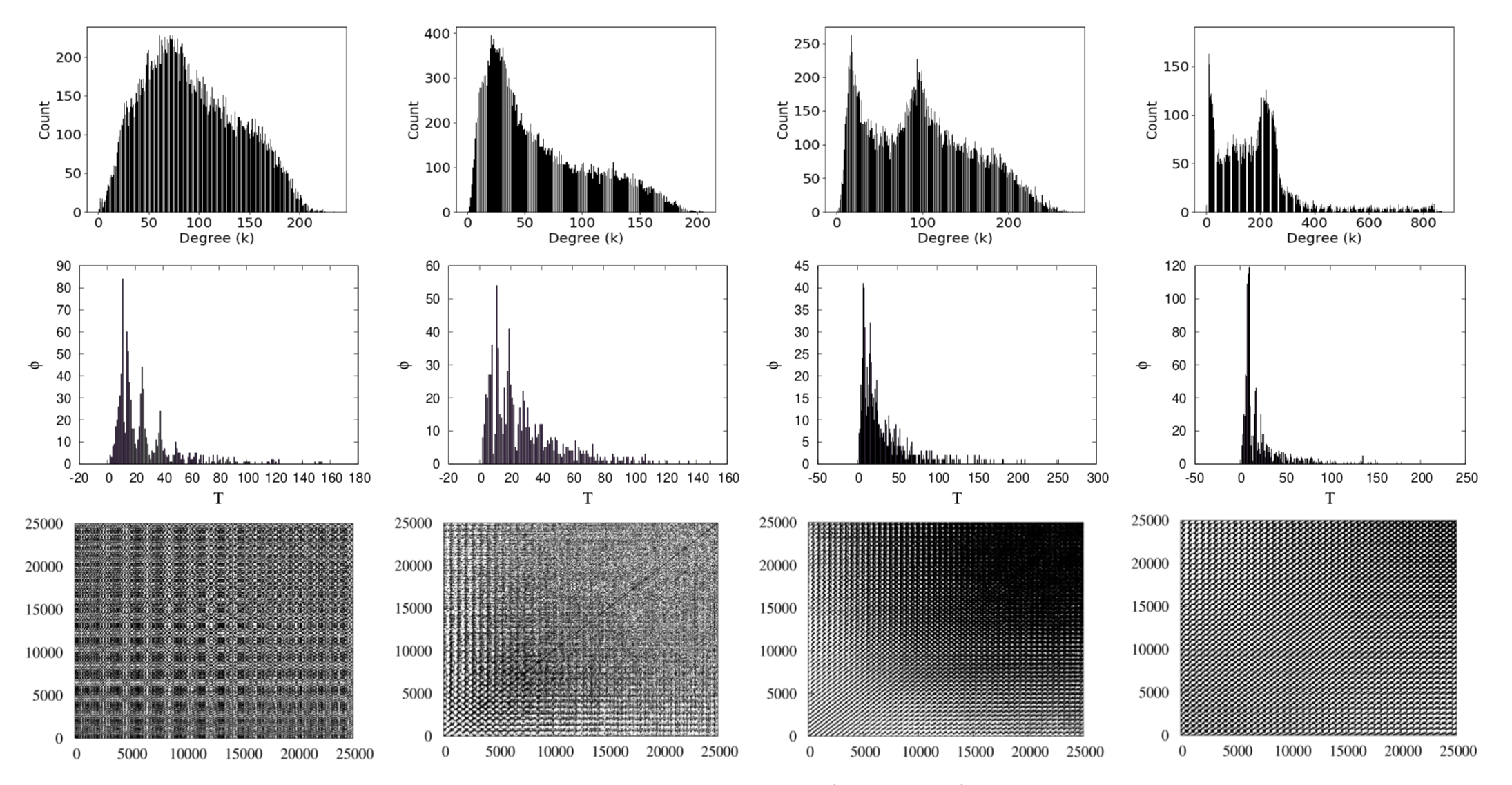
For completeness, we have examined the manner in which the degree distributions, return-time distributions to cells, recurrence plots, etc. vary with changes in in the optomechanical model under study. Each time series comprises 25000 data points. The degree distribution plots are distinctly different for different values of (the top panel of Fig. 6). For instance, the single-peaked distributions for smaller values of gradually change to double-peaked distributions as is increased. Further, the spread in the distributions changes dramatically with increasing .
The first-return-time distributions to a specific cell for various values of are shown in the centre panel of Fig. 6. We find that there exist several significant peaks apart from a prominent peak for almost all values of . For higher value of () the spread in the distribution is relatively smaller. We have verified that the second-return-time distributions exhibit similar behavior.
The manner in which recurrence plots change with is displayed in the bottom panel of Fig. 6. The return maps and the power spectra are not very sensitive to changes in . In the tripartite system, qualitative changes in the recurrence plots, return maps and recurrence-time distributions with changes in the value of mirrored the fact that the MLE was at a minimum at . Such clear signatures are absent in the case of the optomechanical model.
We turn in the next Section to a classical system which is a near analog of the tripartite system, namely, two coupled Duffing oscillators. In this case, it is shown that the variation of the MLE with changes in a parameter analogous to are similar for data sets with points and points respectively, in the sense that both show an overall increase with as is increased (Fig. 7). This feature is akin to that displayed in Fig. 5(a) for the tripartite system, although in that case the sensitivity to the number of data points is significantly lower. It is therefore worth investigating the differences in the behavior of network indicators in these two models.
IV Coupled Duffing oscillators
As mentioned in the Introduction, a classical system comprising two coupled oscillators driven by a harmonic force mimics Garrido Alzar et al. 2002 the phenomenon of EIT manifested in the tripartite quantum system comprising a -atom interacting with two radiation fields. The dynamical equations for the displacements and of the two oscillators are given by
| (16) | ||||
| (17) |
Here, and are damping parameters, is the stiffness parameter, is the coupling parameter, and and are, respectively, the amplitude and angular frequency of the periodic driving force.
In the quantum mechanical counterpart of this system, is the strength of spontaneous emission from the excited state of the -atom, is the energy dissipation rate of the pumping transition, and is the amplitude of the driving field. In practice, of course, nonlinear effects arise. We have therefore considered the modified coupled Duffing equations
| (18) | ||||
| (19) |
where , the strength of the nonlinearity, is analogous to the IDC parameter in the quantum model. As is well known, the forced Duffing oscillator exhibits a very diverse range of complex dynamical behavior, depending on the values of the parameters. For numerical computations we have set the parameters at representative values and = . The dynamical variable considered is the velocity . A long time series of was obtained for various values of with initial conditions .
The manner in which the MLE varies with for and data points respectively (the black curve and the red curve in Fig. 7) reveals that the gross features in the two plots are in reasonable agreement with each other, in contrast to the case of the optomechanical model.
The changes in the behavior of the APL, LD, assortativity, CC and transitivity with varying in are shown in Figs. 8(a)-(d). It is interesting to note that none of these indicators seem to carry any signatures of the behavior of the MLE with . This is in marked contrast to the situation in both the quantum models considered above.
V Concluding remarks
In this work, we have carried out detailed time-series analysis and network analysis on a fully quantum optomechanical model and on a classical model of two interacting Duffing oscillators. Nonlinearities are inherent in both cases: in the former, the intensity-dependent coupling between subsystems; in the latter, a cubic nonlinearity in each oscillator. An archetypal indicator of complex dynamics, the maximal Lyapunov exponent (MLE), has been obtained from the analysis of a long time series in each case. Network analysis of the same systems has been carried out, and network indicators have been estimated from a considerably abbreviated time series. The variations of these quantities with changes in the nonlinearity parameters have been examined extensively and compared with each other. The conclusions drawn on the similarities between these two sets of indicators are also compared with those obtained from earlier investigations on a reference system (another tripartite quantum model comprising a -atom interacting with two radiation fields).
A noteworthy feature that emerges is the following. Network indicators such as the clustering coefficient (CC) and the transitivity capture the behavior of the maximal Lyapunov exponent (MLE) very closely in the quantum system, provided the latter is not very sensitive to the number of data points used, as in the case of the reference system. In the optomechanical model, on the other hand, the MLE is found to be very sensitive to the size of the data set. In this instance, the CC and the transitivity merely capture the overall trend in the MLE reasonably well, without closely following its variation with the nonlinearity parameter. In the classical model considered, while the MLE is not very sensitive to the number of data points used in the analysis, the nonlinearity does not appear in the interaction between subsystems, but only in the individual subsystems. This is the likely reason why none of the network indicators considered displays signatures of the manner in which the MLE changes with the nonlinearity. An important extension of this work would be the identification of other ‘good’ network indicators which reflect in all cases the variations in the MLE when the nonlinearity is tuned, and their sensitivity to the precise form of the nonlinearity. Network analysis would then provide a reliable shorter technique than time-series analysis for determining the salient features of complex dynamical behavior in the expectation values of observables in multipartite quantum mechanical systems.
Acknowledgements.
We acknowledge Soumyabrata Paul for help with some numerical computations in the classical model.References
- Zou et al. (2010) Y. Zou, R. V. Donner, J. F. Donges, N. Marwan, and J. Kurths, Chaos 20, 043130 (2010).
- Gao and Jin (2009) Z. Gao and N. Jin, Phys. Rev. E 79, 066303 (2009).
- Donges et al. (2011) J. F. Donges, R. V. Donner, K. Rehfeld, N. Marwan, M. H. Trauth, and J. Kurths, Nonlinear Proc. Geophys. 18, 545 (2011).
- Marwan et al. (2002) N. Marwan, N. Wessel, U. Meyerfeldt, A. Schirdewan, and J. Kurths, Phys. Rev. E 66, 026702 (2002).
- Ramírez Ávila et al. (2013) G. M. Ramírez Ávila, A. Gapelyuk, N. Marwan, T. Walther, H. Stepan, J. Kurths, and N. Wessel, Philos. Trans. R. Soc. London A 371 (2013).
- Newman (2010) M. Newman, Networks: An Introduction (Oxford University Press, Oxford, 2010).
- Cohen and Havlin (2010) R. Cohen and S. Havlin, Complex Networks: Structure, Robustness and Function (Cambridge University Press, Cambridge, 2010).
- Newman (2003) M. Newman, SIAM Rev. 45, 167 (2003).
- Boccaletti et al. (2006) S. Boccaletti, V. Latora, Y. Moreno, M. Chavez, and D.-U. Hwang, Phys. Rep. 424, 175 (2006).
- Zou et al. (2019) Y. Zou, R. V. Donner, N. Marwan, J. F. Donges, and J. Kurths, Phys. Rep. 787, 1 (2019).
- Lloyd et al. (2016) S. Lloyd, S. Garnerone, and P. Zanardi, Nat. Commun. 7, 1 (2016).
- Rebentrost et al. (2014) P. Rebentrost, M. Mohseni, and S. Lloyd, Phys. Rev. Lett. 113, 130503 (2014).
- Zhang and Small (2006) J. Zhang and M. Small, Phys. Rev. Lett. 96, 238701 (2006).
- Lacasa et al. (2008) L. Lacasa, B. Luque, F. Ballesteros, J. Luque, and J. C. Nuño, Proc. Natl. Acad. Sci. USA 105, 4972 (2008).
- Nicolis et al. (2005) G. Nicolis, C. A. García, and C. Nicolis, Int. J. Bif. Chaos 15, 3467 (2005).
- Marwan et al. (2009) N. Marwan, J. F. Donges, Y. Zou, R. V. Donner, and J. Kurths, Phys. Lett. A 373, 4246 (2009).
- Yang and Yang (2008) Y. Yang and H. Yang, Physica A 387, 1381 (2008).
- Xu et al. (2008) X. Xu, J. Zhang, and M. Small, Proc. Natl. Acad. Sci. USA 105, 19601 (2008).
- Donner et al. (2011) R. V. Donner, J. Heitzig, J. F. Donges, Y. Zou, N. Marwan, and J. Kurths, Euro. Phys. J. B 84, 653 (2011).
- Laha et al. (2019a) P. Laha, S. Lakshmibala, and V. Balakrishnan, Europhys. Lett. 125, 60005 (2019a).
- Abramovici et al. (1992) A. Abramovici, W. E. Althouse, R. W. P. Drever, Y. Gürsel, S. Kawamura, F. J. Raab, D. Shoemaker, L. Sievers, R. E. Spero, K. S. Thorne, R. E. Vogt, R. Weiss, S. E. Whitcomb, and M. E. Zucker, Science 256, 325 (1992).
- Braginsky et al. (1995) V. B. Braginsky, F. Y. Khalili, and K. S. Thorne, Quantum measurement (Cambridge University Press, Cambridge, 1995).
- Vitali et al. (2001) D. Vitali, S. Mancini, and P. Tombesi, Phys. Rev. A 64, 051401 (2001).
- Geraci et al. (2010) A. A. Geraci, S. B. Papp, and J. Kitching, Phys. Rev. Lett. 105, 101101 (2010).
- Lamoreaux (2007) S. K. Lamoreaux, Phys. Today 60, 40 (2007).
- Stannigel et al. (2010) K. Stannigel, P. Rabl, A. S. Sørensen, P. Zoller, and M. D. Lukin, Phys. Rev. Lett. 105, 220501 (2010).
- Barzanjeh et al. (2011) S. Barzanjeh, M. H. Naderi, and M. Soltanolkotabi, Phys. Rev. A 84, 023803 (2011).
- Wilson-Rae et al. (2004) I. Wilson-Rae, P. Zoller, and A. Imamoḡlu, Phys. Rev. Lett. 92, 075507 (2004).
- Genes et al. (2008) C. Genes, D. Vitali, P. Tombesi, S. Gigan, and M. Aspelmeyer, Phys. Rev. A 77, 033804 (2008).
- Li et al. (2008) Y. Li, Y.-D. Wang, F. Xue, and C. Bruder, Phys. Rev. B 78, 134301 (2008).
- Schwab and Roukes (2005) K. C. Schwab and M. L. Roukes, Phys. Today 58, 36 (2005).
- Marshall et al. (2003) W. Marshall, C. Simon, R. Penrose, and D. Bouwmeester, Phys. Rev. Lett. 91, 130401 (2003).
- Aspelmeyer et al. (2014) M. Aspelmeyer, T. J. Kippenberg, and F. Marquardt, Rev. Mod. Phys. 86, 1391 (2014).
- Bowen and Milburn (2016) W. P. Bowen and G. J. Milburn, Quantum Optomechanics (CRC Press, Boca Raton, 2016).
- Sivakumar (2002) S. Sivakumar, J. Phys. A: Math. Gen., 35, 6755 (2002).
- Laha et al. (2019b) P. Laha, S. Lakshmibala, and V. Balakrishnan, J. Opt. Soc. Am. B 36, 575 (2019b).
- Garrido Alzar et al. (2002) C. L. Garrido Alzar, M. A. G. Martinez, and P. Nussenzveig, Am. J. Phys. 70, 37 (2002).
- Argyris et al. (2015) J. Argyris, G. Faust, M. Haase, and R. Friedrich, An Exploration of Dynamical Systems and Chaos (Springer-Verlag Berlin Heidelberg, 2015).
- Harris (1997) S. E. Harris, Phys. Today 50, 36 (1997).
- Fraser and Swinney (1986) A. M. Fraser and H. L. Swinney, Phys. Rev. A 33, 1134 (1986).
- Abarbanel (1996) H. D. I. Abarbanel, Analysis of Observed Chaotic Data (Springer-Verlag New York, 1996).
- Hegger et al. (1999) R. Hegger, H. Kantz, and T. Schreiber, Chaos 9, 413 (1999).
- Eroglu et al. (2014) D. Eroglu, N. Marwan, S. Prasad, and J. Kurths, Nonlinear Proc. Geophys. 21, 1085 (2014).
- Watts and Strogatz (1998) D. J. Watts and S. H. Strogatz, Nature 393, 440 (1998).
- Cleland and Roukes (1996) A. N. Cleland and M. L. Roukes, Appl. Phys. Lett. 69, 2653 (1996).
- Hood et al. (1998) C. J. Hood, M. S. Chapman, T. W. Lynn, and H. J. Kimble, Phys. Rev. Lett. 80, 4157 (1998).