Learning from Noisy Labels with Noise Modeling Network

Learning from noisy labels is an active research topic in the field of machine learning. Current learning approaches can be roughly divided into two categories. The first class of approaches directly learns from data with noisy labels by developing noise robust algorithms Freney14; Kaban12; Natarajan13; Reed14; Liu16. The effect of label noise in model training has been well studied in logistic regression and SVMs Freney14; Kaban12. Natarajan13 developed methods for suitably modifying any surrogate loss function and showed that minimizing the modified loss function on noisy data can provide a performance bound. Reed14 changed the targets label on the fly, in order to reduce the damage from the noisy samples. Liu16 proposed to compute importance weights for training samples and combined them into the loss functions. The second class of approaches are semi-supervised Grandvalet05; Lee13, which assumes some fraction of data has clean labels, while the rest are either unlabeled or have noisy labels. Grandvalet05 added entropy maximization regularization to the unlabeled data to encourage their class predictions with high confidence.

There are limited studies which explicitly address the problem of training a neural network from noisy labels. Most of existing work follows the hidden label framework, but focuses on the multi-class classification task Larsen98; Mnih12; Sukhbaatar15; Xiao15; Goldberger17; Patrini17; Li17; Guan18. Larsen98 models symmetric label noise (i.e. independent of the true label). Sukhbaatar15; Guan18; Bekker16; Patrini17 model asymmetric label noises that are dependent on the true label, but independent of the input features. Xiao15 developed an image-dependent noise model to predict label noise types but their model requires access to a small clean dataset to estimate the label transition matrix. Goldberger17 introduced a feature-dependent noise adaptation layer on top of the softmax to absorb label noise, but it is designed for a single label per image (i.e. multi-class classification). Veit17 presents a label cleaning network, which maps noisy labels to clean labels, and the network is dependent on input features. This approach requires a small fraction of images with clean annotations. The closest work is from Misra16 which proposed a similar noise model for missing labels in multi-label classification, and showed that the complex, human-centric prediction model is better than the simple, visual presence prediction model in missing label scenarios. However, this human-centric prediction model may not work in incorrect label scenarios. In addition, it focuses on improving inference in generating human-centric labels which continues to include labeling noise, instead of predicting clean labels.

Compared to these approaches, our approach more effectively learns a “clean label” multi-label classifier jointly with the noise distribution within the framework of the neural network. We do not assume the availability of any clean labels. Our model resembles a student-teacher model Ba14; Hinton14; Paz16, where a compact or compressed network (student model) is trained to reproduce the output of a deeper network (teacher model). In our case, we train a classifier network with a noise modeling network, where the noise modeling network (teacher) infers the posterior of the hidden true labels during training via backpropagation, as targets for multi-label classifier (student) training.

Our goal is to learn a multi-label classifier given a noisy labeled dataset. Let $\mathcal{I}$ denote an input image or video with observed noisy labels: $\mathbf{z}=[z^{1},\dots,z^{K}]$, where $z^{c}\in\{0,1\}$. $z^{c}$ is an indicator variable denoting whether the input $\mathcal{I}$ is tagged with label $c$. $z^{c}$ can be obtained from annotators, tags from its surrounding texts or keywords from a search engine. $K$ is the total number of possible labels. We denote another indicator variable $y^{c}\in\{0,1\}$ as the unobserved true label indicating whether the label $c$, in fact, belongs to $\mathcal{I}$. Missing label noise for class $c$ occurs when $\mathcal{I}$ is labeled as not belonging to $c$ when in fact, it does (i.e., $z^{c}=0$, $y^{c}=1$ ). Incorrect label noise for class $c$ occurs when $\mathcal{I}$ is tagged with $c$ when in fact, it does not ($z^{c}=1$, $y^{c}=0$). In the case of the noise-free model without the use of the NMN with the true labels $y^{c}$ observable, i.e. $y^{c}=z^{c}$, we can effectively train the MLCN by maximizing the log-likelihood, which takes the form of a cross entropy between provided labels $\mathbf{y}$ and the classifier predicted probabilities $f(\mathcal{I})=[\delta{(o^{1})},\dots,\delta{(o^{K})}]$:

where $\delta{(a)}=1/(1+e^{-a})$ is the sigmoid function and $o^{c}$ is the logit (activation) computed for each class $c$. $\delta{(o^{c})}$ is the estimated probability, i.e $\tilde{p}(y^{c}=1|\mathcal{I})=\delta{(o^{c})}$, Note that in multi-class classification, a softmax would be used to estimate the joint probabilities across classes while in multi-label classification, each label’s probability is determined separately with sigmoid functions.

In the case of noisy annotations, one does not observe $y^{c}$ during the training process. If one simply assumes $y^{c}=z^{c}$ during classifier training, the training process will penalize models that correctly predict a low probability for samples affected by incorrect label noise. This can bias the final classifier to have a higher false positive rate. Similarly, missing label noises may result in a final classifier with higher miss rate. The Noise Modeling Net is needed to address both missing labels and incorrect labels.

Motivated by the noise models in Goldberger17; Bekker16 for the multi-class classification task, here we address missing labels and incorrect labels for multi-label classification by modeling a noise distribution $p(z^{c}=i|y^{c}=j,\mathcal{I})$ in multi-label images.

As shown in Figures 2, our proposed approach augments the training of the Multi-label Classification Net (MLCN) which captures the conditional distribution $p(y^{c}|\mathcal{I})$ of the true label $y^{c}$ given image $\mathcal{I}$ , with the Noise Modeling Net (NMN) which captures the noise distribution $p(z^{c}|y^{c},\mathcal{I})$. To clearly differentiate between the proposed system with NMN and the MLCN, we refer to the full system with NMN as the end-to-end system.

Both the MLCN and the NMN are jointly optimized. Denote $\tilde{p}(z^{c}|\mathcal{I})$ as the estimated probability of the observed label $z^{c}$ and $\tilde{p}(\mathbf{z}|\mathcal{I})=[\tilde{p}(z^{1}|\mathcal{I})...\tilde{p}(z^{K}|\mathcal{I})]$(we use $\tilde{p}$ to denote estimate probabilities and $\mathbf{z}$ for vectors). The log-likelihood of the observed training data $\mathbf{z}$, for a single image $\mathcal{I}$, is the cross entropy given by

$z^{c}$ and $y^{c}$ are connected by an unknown noise distribution $p(z^{c}|y^{c},\mathcal{I})$, where the noisy label is dependent on both the true label and input features; it is the transition probability of noisy label $z^{c}$ from the true label $y^{c}$ given the input $\mathcal{I}$. The estimated feature-dependent noise transition $q^{c}_{ij}$ can be defined as:

where $h(\mathcal{I})$ is the nonlinear function applied on input $\mathcal{I}$ and corresponds to the feature vector $g(X)$ in Figure 2. The variables $u^{c}_{ij}$ and $b^{c}_{ij}$ are the parameters for class $c$ transition between $i$ and $j$. The activation $o^{c}_{ij}=(u^{c}_{ij})^{T}h(\mathcal{I})+b^{c}_{ij}$ is an estimated unnormalized confidence score of transition from true label $j$ to noisy label $i$ for class $c$ (shown as Confidence Map O in Figure 2).

In Bekker16, the noise distribution is assumed to only depend on the true label, independent of the input features. This feature independent transition, $q^{c^{\prime}}_{ij}$ can be obtained by simplifying Equation (3) to

For the rest of the paper, we will continue to use the feature dependent noise distribution with the understanding that it can be simplified to the feature independent case. Using the noise distribution, the estimated probability of observing a noisy label $z^{c}$ given input $\mathcal{I}$ is defined as:

which is the conditional distribution for observing $z^{c}=i$ while $\tilde{p}(y^{c}|\mathcal{I})$ is the estimated true class distribution. The estimated probability, $\tilde{p}(z^{c}=i|\mathcal{I})$, defined in Equation (5), is optimized via Equation (7) and connects the $\tilde{p}(y^{c}=j|\mathcal{I})$ estimated from the MLCN with the $q^{c}_{ij}$ from the NMN.

From Equation (5) and using Bayes rule, we can estimate, $\rho^{c}$, the posterior of the true label $y^{c}$ conditioned on $z^{c}$ by $\rho^{c}=\tilde{p}(y^{c}|z^{c},\mathcal{I})=\frac{\tilde{p}(z^{c}|y^{c},\mathcal{I})\tilde{p}(y^{c}|\mathcal{I})}{\tilde{p}(z^{c}|\mathcal{I})}$. Assuming $\rho^{c}_{ji}=\tilde{p}(y^{c}=j|z^{c}=i,\mathcal{I})$, let’s discuss the properties of ideal MLCN and NMN when processing missing label and incorrect label training instances.

• •

  When encountering training samples with missing label noise (i.e., $z^{c}=0$ and $y^{c}=1$ ), we would be maximizing the log-likelihood of $\log{p(z^{c}=0|\mathcal{I})}$ and the ideal NMN should produce transition probability estimates of $q^{c}_{01}>q^{c}_{00}$ with the MLCN returning $\tilde{p}(y^{c}=1|\mathcal{I})>\tilde{p}(y^{c}=0|\mathcal{I})$. The combination of $q^{c}_{01}>q^{c}_{00}$ and $\tilde{p}(y^{c}=1|\mathcal{I})>\tilde{p}(y^{c}=0|\mathcal{I})$ will imply $\rho^{c}_{10}>\rho^{c}_{00}$.

• •

  Similarly, when training with instances of incorrect label noise, (that is, $z^{c}=1$ and $y^{c}=0$), a higher estimate of $q^{c}_{10}>q^{c}_{11}$ from NMN and MLCN with high confidence of $y^{c}=0$ will maximize the log-likelihood $\log{p(z^{c}=1|\mathcal{I})}$.

These two properties allow the training of a good classifier from data with incorrect and missing label noises. Recall that the end-to-end system is trained by minimizing a cross-entropy loss (equivalent to maximizing the likelihood) between provided noisy labels and observed class distributions $\tilde{p}(z^{c}|\mathcal{I})$. Because our model factorizes over the classes $c$, and there is only a single latent variable $y^{c}$, the derivative of cross entropy loss $L$ with respect to the MLCN activation $o^{c}$ can be found directly. Let’s examine how this derivative behaves under different noise conditions.

In the noise-free scenario with the noise-free model (i.e., $z^{c}=y^{c}$ and without NMN), the likelihood is described in Equation (1). We have $\frac{\partial{L}}{\partial{o^{c}}}\propto y^{c}-\tilde{p}(y^{c}=1|\mathcal{I})$. Effectively, the learning procedure will try to make the prediction $\tilde{p}(y^{c}=1|\mathcal{I})$ as close to true label $y^{c}$ as possible. For the end-to-end model with the NMN, although the likelihood function in Equation (7) is similar to Equation (1), the derivatives of the likelihood against the MLCN parameters have to back-propagate though the NMN.

• •

  In the missing label scenario, the derivative $\frac{\partial{L}}{\partial{o^{c}}}\propto\rho^{c}_{10}-\tilde{p}(y^{c}=1|\mathcal{I})$. That is to say, the training makes the prediction $\tilde{p}(y^{c}=1|\mathcal{I})$ approximate the posterior probability of the true label $y^{c}=1$ given the noisy value $z^{c}=0$ and input $\mathcal{I}$. This will cause the classifier to be penalized less for making a confident but incorrect prediction.

• •

  In the incorrect label scenario, the derivative takes the form of $\tilde{p}(y^{c}=0|\mathcal{I})-\rho^{c}_{01}$. The training encourages the prediction $\tilde{p}(y^{c}=0|\mathcal{I})$ to approximate the posterior probability of the true label $y^{c}=0$ given the observed value $z^{c}=1$ and input $\mathcal{I}$.

• •

  For the correct label scenario, (i.e., $z^{c}=y^{c}=0$ and $z^{c}=y^{c}=1$), their derivatives take the form $\tilde{p}(y^{c}=0|\mathcal{I})-\rho^{c}_{00}$ and $\rho^{c}_{11}-\tilde{p}(y^{c}=1|\mathcal{I})$, respectively.

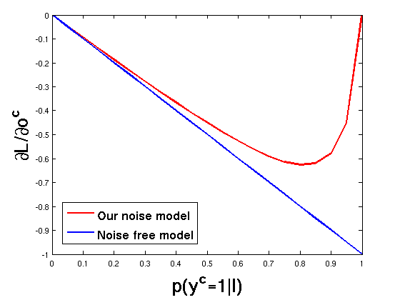
Figure 3 shows how the derivative changes with different values of predictions $\tilde{p}(y^{c}=1|\mathcal{I})$ using the noisy-free model and our noise model under a specific set of $q^{c}_{ij}$. When the model is consistent with the observed label, or $\tilde{p}(y^{c}=z^{c}|\mathcal{I})$ is high, the two models have similar derivatives. However, when the model predicted label for the sample is very different from the observed label—a large $\tilde{p}(y^{c}=1|\mathcal{I})$ for missing label noise and a small $\tilde{p}(y^{c}=1|\mathcal{I})$ for incorrect label noise—the new model reduces the derivatives, reducing the impact of training under errorful labeling. By using the fact that $\sum_{j}\rho^{c}_{ji}=1$, $\sum_{j}\tilde{p}(y^{c}=j|\mathcal{I})=1$ and some algebraic manipulation, we can show that the derivative has the form, $\frac{\partial{L}}{\partial{o^{c}}}\propto\rho^{c}-\tilde{p}(y^{c}=1|\mathcal{I})$. That is to say, the proposed NMN generates the posterior probabilities of the true label $\rho^{c}$ as ‘soft target’ labels to guide the MLCN training.

Since hidden true class label can be considered as a random variable $y^{c}\in\{0,1\}$, as in Goldberger17; Bekker16; Xiao15, we could use the EM algorithm to learn the model parameters, where the E-step estimates the posterior of true labels and the M step updates the parameters of the noise distribution and classifier. However, the EM algorithm is known to get stuck in local optima easily, worse, if a large-scale neural network is used for classifier training, it may lead to slow optimization convergence and the network converging to a poor local minimum. Here we put all of these into an end-to-end deep learning framework and optimize them jointly. In fact, our network optimizes the same likelihood function optimized by EM-based algorithms. The proof is provided in the supplemental material.

We use a neural network to model the observed class distribution $\tilde{p}(z^{c}|\mathcal{I})$ in (5). The overall framework is shown in Figure 2 and consists of two sub-networks: the MLCN and the proposed NMN. MLCN has similar network structure as in fully convolutional VGG16 network Long15 and includes two parts: CNN and a Multi-label Classifier. The CNN includes 15 convolution layers and 5 max-pooling layers while the Multi-label Classifier is modeled as a convolution layer with $K$ kernels of size $1\times 1$ (‘conv(K)’ in Figure 2) and a sigmoid layer. MLCN predicts the true class distribution $\tilde{p}(y^{c}|\mathcal{I})$ and feeds it to the NMN.

The NMN takes a feature map $X$ from the MLCN as inputs, and uses spatial pooling to obtain the input feature vector $g(X)$ (i.e., $h(\mathcal{I})$ in Equation (3)). Then it applies four linear classifiers for pairwise labels ($u^{c}_{ij}$ and $b^{c}_{ij}$) to the input feature vector, where the linear classifiers are modeled as a convolution layer with $4K$ filters of size $1\times 1$ (‘conv(4K)’), and followed by a reshape layer. The output of the reshape layer is a confidence map $O\in\mathbb{R}^{2\times 2\times K}$. Next the confidence map is converted to the noise distribution matrix $Q$ by a softmax layer, which corresponds to the estimation of Equation (3). Next $Q$ is fed into a Transformation layer, which transforms the input true class probabilities $\tilde{p}(y^{c}|\mathcal{I})$ to the observed class probability $\tilde{p}(z^{c}|\mathcal{I})$ by computing a weighed sum of true class probabilities $\tilde{p}(y^{c}=0|\mathcal{I})$ and $\tilde{p}(y^{c}=1|\mathcal{I})$ with weights in noise distribution according to Equation (5). For instance, we used $q^{c}_{10}$ and $q^{c}_{11}$ as weights to compute $\tilde{p}(z^{c}=1|\mathcal{I})$. The whole network is a unified framework and is trained with the cross-entropy loss between noisy labels $z^{c}$ and $\tilde{p}(z^{c}|\mathcal{I})$. At test time, we remove the NMN and only use the MLCN to predict the true label $y^{c}$.

We also add the multiple instance learning (MIL) layer provided by Fang15 to the MLCN. Image MIL considers an input image as a bag $b_{r}$ and image regions as instances of the bag. The MIL layer predicts the probability $\tilde{p}^{c}_{r}$ of a bag containing concept $c$ based on the probabilities $\tilde{p}^{c}_{r,s}$ of individual instances (image regions) in the bag: $1-\prod_{s\in b_{r}}{(1-\tilde{p}^{c}_{r,s})}$. The MIL layer pools together the CNN features computed on the images regions spatially. We extend this approach to videos. We call it Video MIL, where an input video is considered as a bag and each image region from each video frame is an instance in the bag.

MIL can be viewed as an approach to compensating for label noise. Consider the task of training an image classifier from video frames. The individual frames are unlikely to be labeled, so they must be assumed from video-level labels. While a given label may apply to the video as a whole, its evidence may be missing from any given frame; this is analogous to the incorrect label case. With MIL, the label is applied to the bag of frames from the video instead of each individual frame, implicitly correcting for the incorrect label on individual frame.

Our NMN model handles the case where the label is incorrect for the entire bag. In addition, it can directly compensate for missing labels. The MIL layer also implicitly compensates for missing labels at the instance level, but has no mechanism for handling missing labels at the bag level. As we show in Section 3, the two approaches are complementary and the NMN model still improves performance even when MIL layers are utilized.

To evaluate the performance of our approach, we obtain ground-truth labels from each image’s captions. Any word in any of the captions of an image which is in the concept vocabulary is included as a label for the image. Since these labels are from simple, human-annotated image captions, missing labels, on things such as small objects or object attributes, may occur. We measure the word detection performance in terms of average precision as in Fang15.

The results are summarized in Table 1. We observe obvious performance improvements for nouns and adjectives using the proposed noise modeling network. As expected, the input feature-dependent NMN which considers the image content to determine noise distribution, achieved the best performance.

As shown in Table 1, the MIL layer also improves the detection performance since better localization (i.e., scanning different image regions instead of single whole image) of possible objects can help to detect words as described in Fang15. Interestingly, our proposed NMN, which directly handles the missing label noises, can further improve performance, demonstrating the complementary nature of the two algorithms.

To demonstrate our approach’s ability to handle incorrect label noises, we artificially generate incorrect labels for each training image. Note that there are five ground-truth captions for each image in this dataset. We can effectively generate incorrect labels by randomly replacing some of the reference captions by other captions randomly selected from other images. For example, our $20\%$ incorrect label noise case was generated in this fashion: we replace one of the five ground-truth captions by another caption randomly sampled from another image. Similarly, we generated $40\%$, $60\%$ and $80\%$ incorrect label noises for each image by sampling two, three and four captions from other images, respectively. Note that each ground-truth caption of an image may use unique words not used in the other ground-truth captions. Thus, replacing some of the ground-truth captions may also introduce some missing label noises.

The results are summarized in Table 2. Our NMN shows consistent performance improvements over baseline methods (VGG16 and VGG16*) in three levels (20%, 40% and 60%) of incorrect label noise. As shown in the right-most column (All-MIL) of Table 2, we observe that the MIL layer helped to correct the incorrect labels during training since the VGG16 detection results are significantly improved over all different levels of noise. However, combining the NMN with the baseline model trained with the MIL layer further improved performance. VGG16-NMN-FI, while not as good as the VGG16-NMN-FD, is mostly better than the baseline VGG16 except at the 80% level of incorrect label noise. In this extreme noise condition, feature dependent NMN is necessary.

The observed class distribution $\tilde{p}(z^{c}|\mathcal{I})$ is considered as human-centric predictions in Misra16 and works well in missing label scenarios based on their experiments. In order to see whether the observed class distribution works in the incorrect label scenarios, we test this observed class distribution under the 80% incorrect label noise scenario. We got 21.98% and 28.22% mean average precision using the observed class distributions from our VGG16-NMN-FD model trained without MIL layer and with MIL layer, respectively. The results using observed class distribution became worse than using the estimated true class distribution $\tilde{p}(y^{c}|\mathcal{I})$, which is consistent with our expectation.

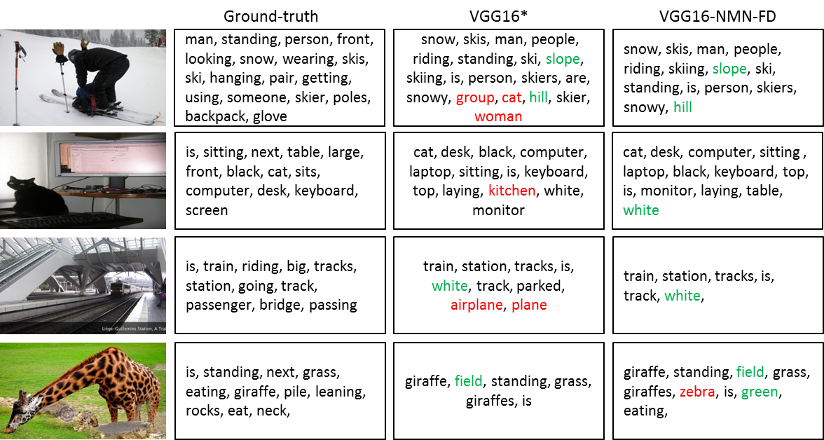
Qualitative results are shown in Figure 4 where these compared models are trained under 40% incorrect label noises. Compared with baseline VGG16*, VGG16-NMN-FD can get better results in word detection since our model can model missing label and incorrect label noise.

We believe incorrect label and missing label noises are common for video concept training. Similar to how we use captions to generate labels for images, we generate the concept labels for each video based on its $20$ video descriptions. The missing label noise is unavoidable since the labels are generated from annotated captions which do not fully describe all the details of the video. To train a concept classifier from videos, a simple and common approach is to extract video frames from each video, and then consider video-level labels as frame-level labels, such as in Shen17. This frame sampling and label assignment strategy will also generate incorrect label noise.

We uniformly extracted $26$ frames from each video, and these $26$-frame video representations are used for both training and testing. We tried two training settings: (1) Frame-level Classifier: we trained a frame-level concept classifier by simply considering video-level labels as frame-level labels. During testing, since the performance evaluation is based on video-level, we obtain a video-level prediction for each testing video by pooling the predictions from the $26$ frames with max-pooling. (2) Video-level Classifier: During training and testing, we aggregated the frame-level predictions across $26$ frames per video to obtain a video-level prediction by using the proposed video MIL layer, an extension of the image MIL layer in Fang15 originally developed for image classification. Here, a video is considered as a bag and all image regions of each video frame are its instances. The video MIL layer pools together the CNN features computed on instances temporally in addition to spatially.

For the frame-level classifier, we added the NMN to the MLCN (VGG16) without using the image MIL layer. For the video-level classifier, each video is considered as a mini-batch and fed into the MLCN, where a video MIL layer and NMN are added. We compared our NMN approach with other two baseline approaches in Table 3. As shown in Table 3, our approach can get better results in these two settings for verbs, nouns and adjectives, which often correspond to concrete regions in an image.

To show the effectiveness and representation power of concepts detected by our approach, we trained a video captioning model based on extracted concept features ($1,087$ concept probabilities). Our video captioning model is the sequence-to-sequence video-to-text (S2VT) model in Venugopalan15, which uses the Long Short Term Memory (LSTM) based encoder-decoder framework to map a sequence of video frames to a sequence of words. We used a vocabulary of $23,647$. The LSTM hidden state size is 700. We embed the input concept features and one-hot representations for caption words to a lower dimensional space, where the parameters of the embedding layers are jointly trained with the LSTM network parameters. The dimensions of the embedded representations for ground-truth caption words and concept features are $300$ and $700$, respectively.

We applied three trained concept models—VGG16*-MIL, VGG16-MIL-NMN-FI and VGG16-MIL-NMN-FD networks from Section 3.3—to extract concept features from each video frame as input features to the LSTM captioning network. As in Ramanishka16; Shen17, we report captioning performance on the validation set in terms of machine translation metrics, including BLEU-4, METEROR, CIDEr and ROUGE-L. In Table 4, we can see that the concept features from the models trained with the NMN can achieve better captioning results compared with VGG16*-MIL, since the NMN enables the MLCN to predict correct and more related concepts from each frame, encouraging the language model to select appropriate input elements based on relevant concepts detected in the frame. Our results are better than state-of-the-art approaches including Shen17; Venugopalan15a; Venugopalan15, and comparable to C3D and ResNet features reported in Ramanishka16. Compared with Yao15, our method outperforms in all metrics except CIDEr.

In this supplementary material, we will describe the EM-based algorithm and end-to-end deep neural network based algorithm, which in fact optimize the same likelihood function. In the training phase, we are given only a noisy image dataset, where each image $\mathcal{I}$ has noisy labels $\mathbf{z}=[z^{1},\dots,z^{K}]$, which are viewed noisy versions of hidden true labels $[y^{1},\dots,y^{K}]$. $z^{c}\in\{0,1\}$ is an indicator variable denoting whether the input $\mathcal{I}$ is tagged with label $c$. $y^{c}\in\{0,1\}$ is another indicator variable indicating whether the label $c$, in fact, belongs to $\mathcal{I}$. $z^{c}$ and $y^{c}$ are connected by an unknown noise distribution $p(z^{c}|y^{c},\mathcal{I})$, which is the transition probability of noisy label $z^{c}$ from the true label $y^{c}$ given the input $\mathcal{I}$.

Our goal is to train a multi-label classification network $p(y^{c}|\mathcal{I};\theta_{1})$, where $\theta_{1}$ is the network parameter set. We follow the EM learning approach described in Bekker16. In Bekker16, the noisy label $z^{c}$ is assumed to be independent of input features and only dependent on the true label $y^{c}$, i.e., $p(z^{c}|y^{c})$. However, $z^{c}$ in our approach is dependent on input features in addition to the true label $y^{c}$, that is, $p(z^{c}|y^{c},\mathcal{I};\theta_{2})$, where $\theta_{2}$ is the noise distribution parameter set. As pointed out in Goldberger17, there is no closed-form solution for $\theta_{2}$ since this noise distribution is input feature dependent, we can apply neural network to model this noise distribution and find the parameters. Therefore we could develop a neural network like our proposed noise modeling network to model noise distribution, and add it on top of the multi-label classification network.

Assuming $\theta=\theta_{1}\cup\theta_{2}$, the log-likelihood of model parameters is:

where $p(z^{c}=1|\mathcal{I};\theta)=\sum_{y^{c}\in\{0,1\}}p(z^{c}=1|y^{c},\mathcal{I};\theta_{2})p(y^{c}|\mathcal{I};\theta_{1})$.

Based on the training data, the goal is to find classification network parameters $\theta_{1}$ and noise distribution parameters $\theta_{2}$ that maximize the likelihood function. Since true label $y^{c}\in\{0,1\}$ is hidden random variable, we can apply EM algorithm to find the maximum-likelihood parameters.

In the E-step, we estimate the posterior of hidden true label $y^{c}$ based on the noise label $z^{c}$ and current classification network parameters $\theta_{1}^{(t)}$ and noise distribution parameters $\theta_{2}^{(t)}$:

In the M-step, we need to optimize $\theta_{1}$ and $\theta_{2}$ given the estimated posterior probabilities of hidden true labels. For $\theta_{1}$, we need to maximize the following auxiliary function:

which can be written as:

Recall $\delta{(o^{c})}=p(y^{c}=1|\mathcal{I};\theta_{1})$, where $o^{c}$ is the logit computed for each class $c$ and $\delta{(o^{c})}$ is the estimated probability, we can easily obtain the derivative of $Q$ with respect to $o^{c}$:

The derivative of $Q(\theta_{1})$ with respect to $\theta_{1}$ can be easily computed using backpropagation from $\frac{\partial{Q(\theta_{1})}}{\partial{o^{c}}}$ we computed. Given the updated classification network parameters $\theta_{1}^{(t+1)}$, we need to maximize the likelihood function in Equation (1) for $\theta_{2}$:

where $p(z^{c}=1|\mathcal{I};\theta_{2},\theta_{1}^{(t+1)})=\sum_{y^{c}\in\{0,1\}}p(z^{c}=1|y^{c},\mathcal{I};\theta_{2})p(y^{c}|\mathcal{I};\theta_{1}^{(t+1)})$. The parameters $\theta_{2}^{(t+1)}$ can be estimated by maximizing this likelihood function.

As described in our paper, we model the observed class distribution $p(z^{c}|\mathcal{I};\theta)$ by an end-to-end deep neural network (DNN) system, which consists of two sub-networks: the Multi-label Classification Net (MLCN) and the proposed Noise Modeling Net (NMN). MLCN captures the conditional distribution $p(y^{c}|\mathcal{I};\theta_{1})$ of the true label $y^{c}$ given image $\mathcal{I}$ , while NMN captures the noise distribution $p(z^{c}|y^{c},\mathcal{I};\theta_{2})$. We can find the network parameters $\theta=\theta_{1}\cup\theta_{2}$ by minimizing the cross entropy between provided noisy labels $\mathbf{z}$ and the estimated probabilities $\tilde{p}(\mathbf{z}|\mathcal{I};\theta)=[\tilde{p}(z^{1}|\mathcal{I};\theta)...\tilde{p}(z^{K}|\mathcal{I};\theta)]$:

Obviously, the EM based algorithm and this deep neural network based algorithm are actually optimizing exactly the same function.

It is sufficient to compute the derivatives of $L(\theta)$ with respect to the logit $o^{c}$, because the derivative of $L(\theta)$ with respect to other neural network parameters can be easily computed using backpropagation from the estimated $\frac{\partial{L(\theta)}}{\partial{o^{c}}}$. We use the chain rule to compute the partial derivative of $L(\theta)$ with respect to the logit $o^{c}$:

where the partial derivative $\frac{\partial{L(\theta)}}{\partial{\tilde{p}(z^{c}|\mathcal{I};\theta)}}=\frac{-1}{\tilde{p}(z^{c}|\mathcal{I};\theta)}$, the partial derivative

and $\frac{\partial{\tilde{p}(y^{c}|\mathcal{I};\theta_{1})}}{\partial{o^{c}}}=\left\{\begin{array}[]{c l}\tilde{p}(y^{c}=0|\mathcal{I};\theta_{1})\tilde{p}(y^{c}=1|\mathcal{I};\theta_{1})&\text{ if $y^{c}=1$},\\ -\tilde{p}(y^{c}=0|\mathcal{I};\theta_{1})\tilde{p}(y^{c}=1|\mathcal{I};\theta_{1})&\text{ if $y^{c}=0$},\end{array}\right.$

Therefore equation (8) can be rewritten as:

By the definition of posterior of true label in equation (2), equation (11) becomes:

By using the fact that $\sum_{y^{c}\in\{0,1\}}\tilde{p}(y^{c}|z^{c},\mathcal{I};\theta)=1$ and $\sum_{y^{c}\in\{0,1\}}\tilde{p}(y^{c}|\mathcal{I};\theta_{1})=1$, it becomes:

We can interpret the derivative with respect to logit $o^{c}$ as encouraging MLCN to approximate the posterior of true label during the training, which is the same as in equation (5) and demonstrates that the two optimization problems are the same. Our main point in this section is that for our end-to-end deep neural network system, the MLCN model parameters $\theta_{1}$ and NMN model parameters $\theta_{2}$ are estimated via stochastic gradient descent during neural network training. We conclude that our end-to-end deep neural network and the EM algorithm are actually optimizing the same function, with the DNN training providing a scalable, practical solution to multi-label learning problems from noisy label datasets.

References

- (1) L. J. Ba and R. Caruana. Do deep nets really need to be deep? In NIPS, 2014.
- (2) R. Barandela and E. Gasca. Decontamination of training samples for supervised pattern recognition methods. In Advances in Pattern Recognition, 2000.
- (3) A. J. Bekker and J. Goldberger. Training deep neural-networks based on unreliable labels. In ICASSP, 2016.
- (4) J. Bootkrajang and A. Kaban. Label-noise robust logistic regression and its applications. In ECML-PKDD, 2012.
- (5) C. E. Brodley and M. A. Friedl. Identifying mislabeled training data. Journal of Artificial Intelligence Research, 11(1):131–167, 1999.
- (6) J. Deng, W. Dong, R. Socher, L.-J. Li, K. Li, and L. Fei-Fei. Imagenet: A large-scale hierarchical image database. In CVPR, 2009.
- (7) H. Fang, S. Gupta, F. Iandola, R. K. Srivastava, L. Deng, P. Dollar, J. Gao, X. He, M. Mitchell, J. C. Plattz, C. L. Zitnick, and G. Zweig. From captions to visual concepts and back. In CVPR, 2016.
- (8) B. Frenay and M. Verleysen. Classification in the presence of label noise: a survey. TNNLS, 25(5):845–869, 2014.
- (9) J. Goldberger and E. Ben-Reuven. Training deep neural-networks using a noise adaptation layer. In ICLR, 2017.
- (10) Y. Grandvalet and Y. Bengio. Semi-supervised learning by entropy minimization. In NIPS, 2005.
- (11) M. Y. Guan, V. Gulshan, A. M. Dai, and G. E. Hinton. Who said what: Modeling individual labelers improves classification. In AAAI, 2018.
- (12) K. He, G. Gkioxari, P. Dollar, and R. Girshick. Mask r-cnn. In ICCV, 2017.
- (13) K. He, X. Zhang, S. Ren, and J. Sun. Deep residual learning for image recognition. In CVPR, 2016.
- (14) G. Hinton, O. Vinyals, and J. Dean. Distilling the knowledge in a neural network. In NIPS Workshop, 2014.
- (15) A. Joulin, L. van der Maaten, A. Jabri, and N. Vasilache. Learning visual features from large weakly supervised data. In ECCV, 2016.
- (16) J. Larsen, L. N. Andersen, M. Hintx-Madsen, and L. K. Hansen. Design of robust neural network classifiers. In ICASSP, 1998.
- (17) Q. V. Le, M. Ranzato, R. Monga, M. Devin, K. Chen, G. S. Corrado, J. Dean, and A. Y. Ng. Building high-level features using large scale unsupervised learning. In ICML, 2012.
- (18) D.-H. Lee. Pseudo-label: The simple and efficient semi-supervised learning method for deep neural networks. In ICML Workshop, 2013.
- (19) Y. Li, J. Yang, Y. Song, L. Cao, J. Luo, and L.-J. Li. Learning from noisy labels with distillation. In ECCV, 2017.
- (20) T.-Y. Lin, M. Maire, S. Belongie, J. Hays, P. Perona, D. Ramanan, P. Dollar, and C. L. Zitnick. Microsoft coco: Common objects in context. In ECCV, 2014.
- (21) T. Liu and D. Tao. Classification with noisy labels by importance reweighting. TPAMI, 38(3):447–461, 2016.
- (22) J. Long, E. Shelhamer, and T. Darrell. Fully convolutional networks for semantic segmentation. In CVPR, 2015.
- (23) D. Lopez-Paz, L. Bottou, B. Scholkopf, and V. Vapnik. Unifying distillation and priviledged information. In ICLR, 2016.
- (24) I. Misra, C. L. Zitnick, M. Mitchell, and R. Girshick. Seeing through the human reporting bias: Visual classifiers from noisy human-centric labels. In CVPR, 2016.
- (25) V. Mnih and G. Hinton. Learning to label aerial images from noisy data. In ICML, 2012.
- (26) N. Natarajan, I. Dhillon, P. Ravikumar, and A. Tewari. Learning with label noises. In NIPS, 2013.
- (27) G. Patrini, A. Rozza, A. K. Menon, R. Nock, and L. Qu. Making deep neural networks robust to label noise: a loss correction approach. In CVPR, 2017.
- (28) L. Pinto, D. Gandhi, Y. Han, Y.-L. Park, and A. Gupta. The curious robot: Learning visual representations via physical interactions. In ECCV, 2016.
- (29) V. Ramanishka, A. Das, D. H. Park, S. Venugopalan, L. A. Hendricks, M. Rohrbach, and K. Saenko. Multimodal video description. In ACM-MM, 2016.
- (30) S. Reed, H. Lee, D. Anguelov, C. Szegedy, D. Erhan, and A. Rabinovich. Training deep neural networks on noisy labels with bootstrapping. In arXiv: 1412.6596, 2014.
- (31) Z. Shen, J. Li, Z. Su, M. Li, Y. Chen, Y.-G. Jiang, and X. Xue. Weakly supervised dense video captioning. In CVPR, 2017.
- (32) C. Su, S. Zhang, J. Xing, W. Gao, and Q. Tian. Deep attributes driven multi-camera person re-identification. In ECCV, 2016.
- (33) S. Sukhbaatar, J. Bruna, M. Paluri, L. Bourdev, and R. Fergus. Training convolutional networks with noisy labels. In ICLR, 2015.
- (34) A. Veit, N. Alldrin, G. Chechik, I. Krasin, A. Gupta, and S. Belongie. Learning from noisy large-scale datasets with minimal supervision. In CVPR, 2017.
- (35) S. Venugopalan, M. Rohrbach, J. Donahue, R. Mooney, T. Darrell, and K. Saenko. Sequence to sequence – video to text. In ICCV, 2015.
- (36) S. Venugopalan, H. Xu, J. Donahue, M. Rohrbach, R. Mooney, and K. Saenko. Translating videos to natural language using deep recurrent neural networks. In NAACL-HLT, 2015.
- (37) X. Wang and A. Gupta. Unsupervised learning of visual representations using videos. In ICCV, 2015.
- (38) T. Xiao, T. Xia, Y. Yang, C. Huang, and X. Wang. Learning from massively noisy labeled data for image classification. In CVPR, 2015.
- (39) J. Xu, T. Mei, T. Yao, and Y. Rui. Msr-vtt: A large video description dataset for bridging video and language. In CVPR, 2016.
- (40) L. Yao, A. Torabi, K. Cho, N. Ballas, C. Pal, H. Larochelle, and A. Courville. Describing videos by exploiting temporal structure. In ICCV, 2015.
Appendix
Proof of deep neural networks with noise modeling network (NMN) optimizing the same likelihood function as the noise modeling approach by expectation-maximization (EM) algorithm