Predicting Cosmological Observables with PyCosmoJournal: Astronomy and Computing

F.Tarsitano Address: Institute for Particle Physics and Astrophysics, Department of Physics, ETH Zurich, Wolfgang-Pauli-Strasse 27, 8093 Zurich, Switzerland U.Schmitt Address: Institute for Particle Physics and Astrophysics, Department of Physics, ETH Zurich, Wolfgang-Pauli-Strasse 27, 8093 Zurich, Switzerland A.Refregier Address: Institute for Particle Physics and Astrophysics, Department of Physics, ETH Zurich, Wolfgang-Pauli-Strasse 27, 8093 Zurich, Switzerland J.Fluri Address: Institute for Particle Physics and Astrophysics, Department of Physics, ETH Zurich, Wolfgang-Pauli-Strasse 27, 8093 Zurich, Switzerland R.Sgier Address: Institute for Particle Physics and Astrophysics, Department of Physics, ETH Zurich, Wolfgang-Pauli-Strasse 27, 8093 Zurich, Switzerland A.Nicola Address: Department of Astrophysical Sciences, Princeton University, Princeton, NJ 08544, USA J.Herbel Address: Institute for Particle Physics and Astrophysics, Department of Physics, ETH Zurich, Wolfgang-Pauli-Strasse 27, 8093 Zurich, Switzerland A.Amara Address: Institute for Particle Physics and Astrophysics, Department of Physics, ETH Zurich, Wolfgang-Pauli-Strasse 27, 8093 Zurich, Switzerland T.Kacprzak Address: Institute for Particle Physics and Astrophysics, Department of Physics, ETH Zurich, Wolfgang-Pauli-Strasse 27, 8093 Zurich, Switzerland L.Heisenberg Address: Institute for Theoretical Physics, ETH Zurich, Wolfgang-Pauli-Strasse 27, 8093, Zurich, Switzerland

Abstract

Current and upcoming cosmological experiments open a new era of precision cosmology, thus demanding accurate theoretical predictions for cosmological observables. Because of the complexity of the codes delivering such predictions, reaching a high level of numerical accuracy is challenging. Among the codes already fulfilling this task, PyCosmo is a Python-based framework providing solutions to the Einstein-Boltzmann equations and accurate predictions for cosmological observables. In this work, we first describe how the observables are implemented. Then, we check the accuracy of the theoretical predictions for background quantities, power spectra and Limber and beyond-Limber angular power spectra by comparison with other codes: the Core Cosmology Library (CCL), CLASS, HMCode and iCosmo. In our analysis we quantify the agreement of PyCosmo with the other codes, for a range of cosmological models, monitored through a series of unit tests. PyCosmo, conceived as a multi-purpose cosmology calculation tool in Python, is designed to be interactive and user-friendly. A current version of the code (without the Boltzmann Solver) is publicly available and can be used interactively on the platform PyCosmo Hub, all accessible from this link: (https://cosmology.ethz.ch/research/software-lab/PyCosmo.html). On the hub the users can perform their own computations using Jupyter Notebooks without the need of installing any software, access to the results presented in this work and benefit from tutorial notebooks illustrating the usage of the code. The link above also redirects to the code release and documentation.

Keywords:

cosmology , theory , models , Python

1 Introduction

Present research in cosmology investigates the validity of the $\Lambda$ CDM model and its extensions by testing its parameters through observational probes, such as the Cosmic Microwave Background (CMB), Baryonic Acoustic Oscillations (BAO), weak lensing, cluster counts, supernovae and galaxy surveys. The combination of these observables has high constraining power on the parameters of these cosmological models. Current and upcoming cosmological experiments, such as DES¹¹ 1 http://www.darkenergysurvey.org, DESI²² 2 http://desi.lbl.gov, LSST³³ 3 http://www.lsst.org, Euclid⁴⁴ 4 http://sci.esa.int/euclid/ and WFIRST⁵⁵ 5 http://wfirst.gsfc.nasa.gov aim at precise measurements of these observables, thus demanding highly accurate theoretical predictions. Codes fulfilling this task are already available, such as COSMICS [Bertschinger 1995], CMBFAST [Seljak and Zaldarriaga 1996a], CMBEASY [Doran 2005], CAMB [Lewis et al. 2000], CLASS [Lesgourgues 2011], iCosmo [Refregier et al. 2011], CosmoLike [Krause and Eifler 2017], CosmoSIS [Zuntz et al. 2015], CCL [Chisari et al. 2019]. PyCosmo [Refregier et al. 2018] is a recently introduced Python-based framework which provides cosmological model predictions, fitting within the upcoming new era of precision cosmology. As a Boltzmann solver, it computes solutions to the set of Einstein-Boltzmann equations, which govern the linear evolution of perturbations in the Universe. These calculations are at the core of most cosmological analyses. PyCosmo introduces a novel architecture that uses symbolic calculations. As described in a previous work [Refregier et al. 2018] the code, based on the Python library Sympy [Meurer et al. 2017], uses computer algebra capabilities to produce fast and accurate solutions to the set of Einstein-Boltzmann equations, and provides the user a convenient interface to manipulate the equations and implement new cosmological models.
In this paper, we present PyCosmo as a more general cosmology code, providing accurate predictions for cosmological quantities, defined in terms of background computations, linear and non-linear perturbations and observables. The fitting functions for the linear and non-linear power spectrum, which are used to compute predictions for angular power spectra with the Limber Approximation [LoVerde and Afshordi 2008], have been extensively tested. In particular we refer to the Halofit fitting function [Smith et al. 2003, Takahashi et al. 2012] and to a revised version of the Halo Model, presented in Mead et al. 2015 as a more accurate function which also accounts for baryonic feedback; below in this section we will refer to it as the Mead et al. model. Both fitting functions within PyCosmo have been used in the MCCL analysis of the DES data described in Kacprzak et al. 2019. The CMB angular power spectrum is computed using the approach of line-of-sight integration proposed in Seljak and Zaldarriaga 1996b.
In order to assess the accuracy of such computations it is important to compare PyCosmo to other available codes, with the aim of obtaining the highest possible agreement between algorithms with independent implementations. In PyCosmo such comparisons are constantly monitored through a system of unit tests. Conceived as a user-friendly code, the currently tested and validated version of PyCosmo is currently available on a public hub, called PyCosmo Hub and accessible from https://cosmology.ethz.ch/research/software-lab/PyCosmo.html. This server hosts several Jupyter notebooks showing how to use PyCosmo by including tutorial-notebooks and examples. Registered users can use PyCosmo for their own calculations without the need of local installations. More details about the hub will be provided later in Section 3.1.
This paper focuses on the implementation of the cosmological observables and the tests made in order to check their accuracy. In this context PyCosmo is compared to the following codes (see also Chisari et al. 2019 for an earlier comparison of some of these codes):

1.

CLASS [Lesgourgues 2011], a C-based Boltzmann solver widely used to compute theoretical predictions, and its python wrapper, classy;
2.

iCosmo [Refregier et al. 2011], an earlier cosmology package written in IDL;
3.

Core Cosmology Library [Chisari et al. 2019], developed within the LSST Dark Energy Science Collaboration [LSST Dark Energy Science Collaboration 2012];
4.

HMCode [Mead et al. 2015], the original implementation of the Mead et al. model, coded in Fortran.

In Section 2 we give an overview of the cosmological observables implemented in PyCosmo. Section 3 describes how they are implemented, providing details concerning the code architecture. Information about the PyCosmo Hub is also provided. In Section 4 we describe the setup and the conventions used for code comparison and we present the main results from those tests.

2 Cosmological model

In this section we give definitions for the cosmological models implemented in PyCosmo. The current version of the code supports a $\Lambda$ CDM cosmology, defined in terms of the matter density components $\Omega_{b}$ and $\Omega_{m}$ , the Hubble parameter $H_{0}$ , spectral index $n_{s}$ , normalization of the density fluctuations $\sigma_{8}$ and a dark energy model with equation-of-state $w=-1$ . The curvature is defined by $\Omega_{k}=1-\sum_{i}\Omega_{i}$ , where $i$ refers to matter ( $\Omega_{m}$ ), radiation ( $\Omega_{r}$ ) and vacuum ( $\Omega_{\Lambda}$ ) density components.

2.1 Background

Background computations start with the calculation of the Hubble parameter, $H(a)$ , and the cosmological distances. The basis of such calculations is the Friedmann equation, obtained by applying the Einstein’s equations to the FLRW metric:

\left(\frac{1}{a}\frac{da}{dt}\right)^{2}=\frac{8\pi G}{3}\rho+\frac{(1-\Omega)H_{0}^{2}}{a^{2}}.

(1)

In this equation $G$ is the Newton’s constant, $\rho$ is the total energy density and $\Omega$ is the sum of matter, radiation and vacuum densities expressed in units of critical density, $\rho_{c}$ , as follows:

\Omega\equiv\Omega_{m}+\Omega_{r}+\Omega_{\Lambda},\ \text{where}\ \Omega_{i}\equiv\rho_{i}/\rho_{c}.

(2)

The critical density is defined as $\rho_{c}\equiv\frac{3H_{0}^{2}}{8\pi G}$ , where $H_{0}$ is the present value of the Hubble parameter: $H_{0}\equiv 100\ h\ km\ s^{-1}Mpc^{-1}$ . The Hubble parameter, in turn, parametrises the expansion rate of the Universe:

\frac{H}{H_{0}}=\left[\Omega_{r}a^{-4}+\Omega_{m}a^{-3}+\Omega_{k}a^{-2}+\Omega_{\Lambda}\right]^{\frac{1}{2}}.

(3)

Cosmological distances contribute to the computation of observables, so we need accurate predictions for those. A first comoving distance is the comoving radius, $\chi$ . Out to an object at scale factor $a$ (or, equivalently, at redshift $z=(1/a)-1$ ) it is defined as follows:

\chi(a)=\int_{a}^{1}\frac{da^{\prime}}{a^{2}H(a^{\prime})}.

(4)

Using the comoving radius PyCosmo evaluates the comoving angular diameter distance, $r$ , as:

r(\chi)=\begin{cases}R_{0}sinh(\frac{\chi}{R_{0}}),\ open\\ \chi,\ \ \ \ \ \ \ \ \ \ \ \ \ \ \ flat\\ R_{0}sin(\frac{\chi}{R_{0}}),\ \ \ closed,\end{cases}

(5)

where $R_{0}$ is the present value scale radius. The scale radius is defined as $\frac{R}{R_{0}}=a=(1+z)^{-1}$ and $R_{0}=\frac{c}{\kappa H_{0}}$ , where $c$ is the speed of light and $\kappa$ is defined as follows:

\kappa^{2}=\begin{cases}1-\Omega,\ open\\ 1,\ \ \ \ \ \ \ flat\\ \Omega-1,\ closed.\end{cases}

(6)

The comoving angular diameter distance is related to the angular diameter distance, $D_{A}$ , and the luminosity distance, $D_{L}$ , according to $D_{A}=a^{2}D_{L}=ar(\chi)$ . The luminosity distance, in turn, is used to compute the distance modulus, $\mu=5log_{10}(D_{L}/pc)-5$ .

2.2 Linear perturbations

2.2.1 Growth of perturbations

PyCosmo computes the linear growth factor of matter perturbations, $D(a)$ , observing that for sub-horizon modes ( $k\gg\eta^{-1}$ ) and at late times ( $a\gg a_{eq}$ ), we can derive, from the Einstein-Boltzmann equations:

\frac{d^{2}\delta_{m}}{da^{2}}+\left(\frac{dlnH}{da}+\frac{3}{a}\right)\frac{d\delta_{m}}{da}-\frac{3\Omega_{m}H_{0}^{2}}{2a^{5}H^{2}}\delta_{m}=0.

(7)

Then the growth factor is computed by integrating the differential equation, and normalised so that $D(a)=a$ in the matter dominated case and $D(a)=1$ when $a=1$ . Another approach to compute the linear growth factor is implemented in PyCosmo and makes use of hypergeometric functions. This formalism is valid for $\Lambda$ CDM only. In Section 4 we will show the results of the code comparison using both methods.

2.2.2 Linear matter power spectrum

Theoretical predictions for cosmological observables require knowledge of the matter distribution in the Universe, both at small and large scales. Given the matter density field, $\rho$ , we can write it in terms of its mean matter density, $\bar{\rho}(t)$ , and the statistical matter density perturbations:

\delta(\textbf{x},t)=\frac{\rho(\textbf{x},t)-\bar{\rho(t)}}{\bar{\rho(t)}}.

(8)

We are interested in the Fourier space overdensity, $\tilde{\delta(\textbf{k})}$ , which is the Fourier transform of the density fluctuations. The power spectrum, $P(k)$ , is given by the average of overdensities in Fourier-space:

\langle\tilde{\delta}(\textbf{k})\tilde{\delta}(\mathbf{k^{\prime}})\rangle=(2\pi)^{3}P(k)\delta^{3}(\textbf{k}-\mathbf{k}^{\prime}),

(9)

where $\delta^{3}$ is the Dirac delta function.
In addition to the Boltzmann Solver solution for the linear power spectrum, other approaches are used, typically based on numerical simulations. In this context approximate functions have been proposed. The fitting functions implemented in PyCosmo for the linear power spectrum are the Eisenstein $\&$ Hu, described in Eisenstein and Hu 1998, and a polynomial fitting function, namely BBKS [Peacock 1997].

2.3 Non-linear perturbations

As briefly described above, on large scales (small $k$ ) the power spectrum can be calculated from linear perturbation theory. On small scales, evolving structures in the Universe become non-linear and perturbation theory breaks down. In analogy to the approximate functions for the linear power spectrum, also the non-linear power spectrum can be computed using fitting functions, following the same approach based on numerical simulations. A recently developed method, described in Bartelmann et al. 2016 and Bartelmann et al. 2017, proposes the prediction of the non-linear power spectrum without using N-body simulations, but through non-perturbative analytical computation. We describe below the two non-linear fitting functions implemented in PyCosmo, Halofit [Smith et al. 2003, Takahashi et al. 2012] and the model proposed in Mead et al. 2015 and originally implemented in the HMCode. Future code developments will also explore the analytical approach.

2.3.1 Non-linear power spectrum

The Halo Model describes the dark matter density field as a superposition of spherically symmetric haloes, with mass function and internal density structure derived from cosmological simulations. The power spectrum can be written as:

P(k)=P_{1H}(k)+P_{2H}(k),

(10)

where $P_{1H}(k)$ and $P_{2H}(k)$ are denoted the one-halo and two-halo term, respectively. The first relates to the profile of the spherical haloes, while the second accounts for their spatial distribution, considering that their positions are correlated. For more details concerning the Halo Model we refer the reader to Peacock and Smith 2000, Seljak 2000, Cooray and Sheth 2002. The non-linear fitting functions implemented in PyCosmo are described below.

HaloFit

Predictions for the non-linear matter power spectrum, following the fitting function Halofit [Smith et al. 2003] and its revisions presented in Takahashi et al. 2012, are both implemented in PyCosmo. Both papers propose the formalism described in eq. 10, where each term is a parametric function. The revised model provides updated fitting parameters, based on more accurate simulations.

Mead et al. model

PyCosmo includes a first Python implementation of a revised version of the Halo Model, to which we already referred as the Mead et al. model [Mead et al. 2015], originally implemented in the HMCode. In this model physically-motivated new parameters are added to the Halo Model formalism, in particular a smoothing parameter between the one-halo and the two-halo terms, and further parameters used to describe the effects of baryonic feedback on the power spectrum. The latter are found from a set of high-resolution N-body simulations and from OWLS hydrodynamical simulations which investigate the effect of baryons. As in the original HMcode, three different models accounting for baryons are available: a more general model including prescriptions for gas cooling and heating, star formation and evolution and supernovae feedback, called REF; a model which adds to REF the AGN feedback, called AGN; and a model which is similar to REF, called DBLIM, which includes a more complete treatment of the supernovae feedback, described in Van Daalen et al. 2011. For more detailed information about these models and how they are defined in the HMcode, we refer the reader to Mead et al. 2015. In terms of computational speed, part of the PyCosmo code has been implemented in cython to speed up the computations. PyCosmo and the HMCode run at comparable speeds.

2.4 Observables

2.4.1 Angular power spectrum with the Limber Approximation

Many observables in cosmology are expressed in terms of angular correlation functions of random fields, or their spherical harmonic transform, the angular power spectrum. Its calculation gives expressions including several integrals which require numerical evaluation. In order to simplify them, we can use approximation methods, such as the Limber Approximation [Limber 1953, Kaiser 1992, Kaiser 1998, Loverde and Afshordi 2008]. This prescription is implemented in PyCosmo. In particular, the weak lensing shear power spectrum is expressed as:

C_{\ell}=\frac{9}{16}\left(\frac{H_{0}}{c}\right)^{4}\Omega_{m}^{2}\int_{0}^{\chi_{h}}d\chi\left[\frac{g(\chi)}{ar(\chi)}\right]^{2}P\left(\frac{l}{r},\chi\right),

(11)

where $\chi$ is the comoving distance and $\chi_{h}$ the comoving distance to the horizon. $g(\chi)$ is the lensing radial function, which is defined in terms of $p_{\chi}(\chi)$ , the probability of finding a galaxy at a comoving distance $\chi$ :

g(\chi)=2\int_{\chi}^{\chi_{h}}d\chi^{\prime}p_{\chi}(\chi)\frac{r(\chi)r(\chi^{\prime}-\chi)}{r(\chi^{\prime})},

(12)

where $p_{\chi}(\chi)$ is normalised as $\int d\chi p_{\chi}(\chi)=1$ .
In this work we use the lensing power spectrum, $C_{\ell}^{\gamma\gamma}$ , as an example of observable.

2.4.2 Line-Of-Sight integrals

The Boltzmann Solver includes a first python implementation of the $C_{\ell}^{TT}$ , using the line-of-sight integration. In this method, described in detail in Seljak and Zaldarriaga 1996b, the temperature field is a time integral over the product of a source term and a spherical Bessel function, therefore splitting between the dynamical and geometrical effects on the anisotropies. The source function, which can be computed semi-analytically, is defined as follows:

S(k,\eta)=g\left(\Theta_{0}+\Psi+\frac{\dot{u}_{b}}{k}+\frac{\Pi}{4}+\frac{3\ddot{\Pi}}{4k^{2}}\right)+\dot{g}\left(\frac{u_{b}}{k}+\frac{6\dot{\Pi}}{4k^{2}}\right)+\ddot{g}\left(\frac{3\Pi}{4k^{2}}\right)+e^{-\tau}\left(\dot{\Psi}-\dot{\Phi}\right),

(13)

where $g(\eta)$ is the visibility function, defined in terms of the optical depth as $g(\eta)=-\dot{\tau}e^{-\tau}$ . The terms in $\Theta_{0}+\Psi$ , $u_{b}$ and $\Pi$ are the Sachs-Wolfe, Doppler and polarization terms, respectively, while the $\dot{\Psi}-\dot{\Phi}$ term describes the Integrated Sachs-Wolfe effect.
The temperature field is computed along the line of sight as:

\Theta_{\ell}(k,\eta)=\int_{0}^{\eta_{0}}d\eta S(k,\eta)j_{\ell}[k(\eta_{0}-\eta)],

(14)

where $j_{\ell}(\eta)$ is the spherical Bessel function of $\ell$ order. The temperature field, normalized to the density perturbations for dark matter at present time ( $\delta_{0}$ ), is integrated over the wave-numbers to get the angular power spectrum:

C_{\ell}^{TT}=\frac{2}{\pi}\int dk\ k^{2}P(k)\left|\frac{\Theta_{\ell}(k)}{\delta_{0}(k)}\right|^{2},

(15)

where $P(k)$ is the linear power spectrum computed at present time.

3 Implementation

3.1 Architecture

The flow chart in Figure 1 shows the code architecture. After instantiating PyCosmo, the user can set the cosmology through a set-function which or, equivalently, an internal configuration file. The latter can be modified also to choose the method to compute the matter power spectra. The Background class computes basic background quantities, such as the Hubble parameter and comoving distances. The Linear Perturbations class provides the linear power spectrum either through the Boltzmann Solver or through fitting functions. The output is then used to compute the non-linear power spectrum in the Non-linear Perturbations class. In turn, this module offers a choice of different fitting functions. The power spectrum is involved in computing the observables by the class Observables. The theoretical models implemented in this routine are described in Section 2.

Refer to caption — Figure 1: Flow-chart summarizing the PyCosmo architecture. From the top: Cosmological parameters refers to the initial cosmological setup, which affects all the computations. The Background class computes the Hubble parameter and comoving distances. It is followed by the Linear Perturbations and Non-linear Perturbations modules, which include various methods to compute matter power spectra (described in Section 2). The Observables module at the end of the chart calls all the other modules before.

3.2 Symbolic calculations

As shown in the flow-chart in Figure 1, one of the classes implemented in PyCosmo provides solutions to the set of Einstein-Boltzmann equations, which govern the linear evolution of perturbations in the Universe. The novelty of this solver is its approach to the equations themselves, which are symbolically represented through the Python package Sympy. The symbolic representation provides the user a convenient interface to manipulate the equations and implement new cosmological models. The equations are then simplified by a C++ code generator before being evaluated. For more details about how the solver computes a numerical solution for them, we refer the user to a previous work, Refregier et al. 2018, which focusses on the PyCosmo Boltzmann solver.

3.3 Unit tests

Each class shown in Figure 1 is associated with a unit-test routine. It consists in a series of functions testing the methods implemented in each class. These tests perform code-comparison between PyCosmo and the other codes, and check whether the agreement passes a certain numerical accuracy. Every time the code is updated, the developer can check through unit-tests also the impact the new implementations might have on pre-existing parts of the code. The analysis presented later in Section 4 shows the results of code-comparison which is incorporated in the unit-tests. The coverage refers to the amount of code tested and validated in each module through unit-tests. Currently the PyCosmo modules have the following coverage: $100\%$ for the Background class, $91\%$ for the Linear Perturbations, $96\%$ for the Non Linear Perturbations using the Halofit fitting function, $95\%$ for the Non Linear Perturbations using the HMCode model and $96\%$ for the Observables class.

3.4 PyCosmo Hub

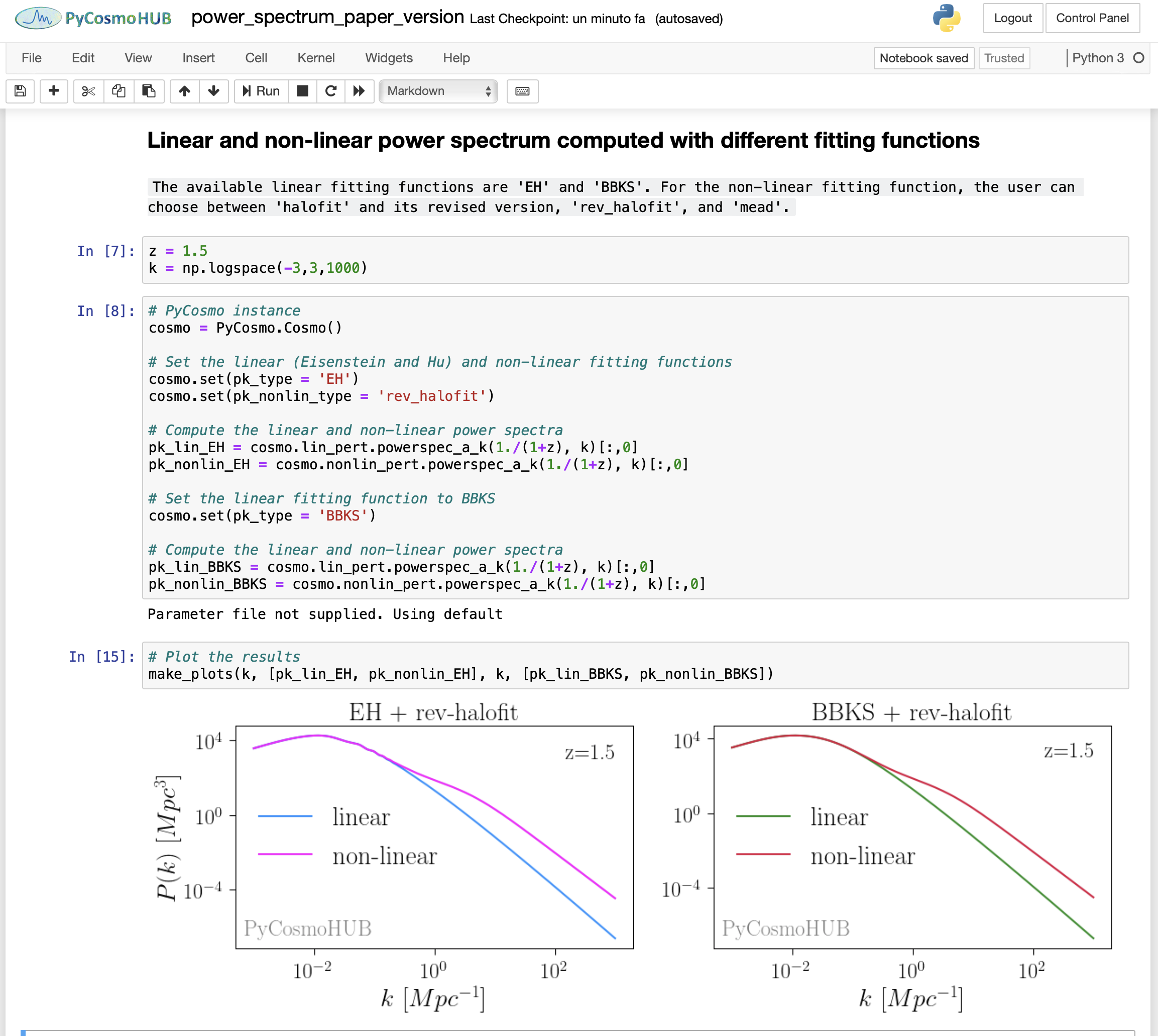
PyCosmo is conceived as a multi-purpose cosmology calculation tool in Python, and designed to be interactive and user-friendly. As discussed above, the usage of the Sympy package is part of this concept. Indeed, PyCosmo is user-friendly not only in its numerical implementation, but also in terms of its public interface: in order to make its usage immediate to the user, we make PyCosmo publicly available on a hub platform, called PyCosmo Hub (see a screenshot in Fig.2). Its current version, accessible from this link, https://pycosmohub.phys.ethz.ch/hub/login, includes Jupyter tutorial-notebooks illustrating how to use the code and shows the results of the code-comparison analysis through a series of static notebooks. The hub currently hosts the most recent versions of the codes CLASS and iCosmo, which can be run by the users. The iCosmo code, originally written in IDL language, is interpreted on the hub through GDL, an open source library alternative to IDL. The PyCosmo version installed on the hub can be downloaded via $pip$ . Further information about the code release and documentation is available on this web page: (https://cosmology.ethz.ch/research/software-lab/PyCosmo.html. The users accessing the hub have space to write their own notebooks, make their own calculations and save the results locally, without the need of installing any software. In this context, the hub is conceived to be useful both for educational purposes and for promoting cosmological inferences in the cloud, in a new dynamic way of teaching and doing research.

4 Validation and code comparison

In order to assess the level of accuracy in the computation of cosmological observables, PyCosmo monitors its own predictions internally and making comparisons with other cosmology codes. The reliability of every function in PyCosmo is checked through unit tests, described in Section 3.3. In this section, we show the main results from those tests: overall we obtain a good agreement between the codes, both using a fiducial cosmology and testing their response by varying the cosmological setup. We compare the algorithms also in terms of execution speed, with the result that PyCosmo runs at a speed comparable with the other codes.

4.1 Cosmological setup and conventions

The tests performed to assess the agreement between the codes are of two kinds, either referring to a fiducial cosmological setup or testing the robustness of the code to changes of cosmological parameters. We assume as our fiducial cosmology: $h=0.7,\ \Omega_{m}=0.3,\ \Omega_{b}=0.06,\ \Omega_{c}=0.24,\ n_{s}=1,\ \sigma_{8}=0.8,\ N_{\rm{eff}}=3$ . We vary cosmology in ranges of $h$ and $\Omega_{m}$ : $h\in[0.4,0.9]$ , $\Omega_{m}\in[0.2,0.7]$ , and we produce heatmaps to show the agreement between the codes across the $(h,\Omega_{m})$ parameter space. In this section we include the heatmaps only for the background computations and for the linear and non-linear power spectra, showing those for the other classes in Appendix B.

To illustrate trends as a function of redshift in our fiducial cosmology, for instance in terms of background quantities (cosmological distances, linear growth factor), we consider a redshift range of $z\in[0,9.5)$ with 5000 grid points. If we vary the cosmological parameters, we consider redshift in the range $[0,6)$ , maintaining the same number of points. When we compare the non-linear power spectrum to the HMcode, we compute it as a function of wavenumbers, $k$ , logarithmically spaced between $10^{-3}$ and $10^{4}Mpc^{-1}$ , with a total of 200 points. When we compare the power spectra predicted by different codes we use 200 wavenumbers logarithmically spaced between $10^{-3}$ and $10^{3}Mpc^{-1}$ , which is the sampling used by default in iCosmo. Testing the angular power spectrum, we choose a sample of multipoles, $\ell$ , linearly spaced between $10$ and $10^{4}$ , following also in this case the convention adopted in iCosmo.
In each test, the setup described above is matched between the codes, but there are further parameters which need special care in order to make consistent tests. A detailed description of their configuration is given in Appendix A.

In the next paragraphs, we show the results of the code comparisons. The achieved accuracy is quantified in terms of the relative difference between two compared quantities (i.e. distances, power spectra etc.). Given $Q$ a certain cosmological quantity we consider for comparison between PyCosmo and a code $C$ , the accuracy is defined as follows:

A=\frac{|Q_{\textsf{PyCosmo}}-Q_{C}|}{Q_{\textsf{PyCosmo}}},

(16)

and it is always reported in logarithmic scale. $A$ is a vector including as many points as the two compared quantities. In the heatmaps summarizing the results when varying cosmology, each cell refers to a particular combination of $(h,\Omega_{m})$ . It is colour-coded by the base-10 logarithm of the maximum accuracy ( $Log[MAX(A)]$ ) and labelled by the dispersion in accuracy ( $\sigma(A)$ ) obtained for the specific cosmological setup it represents. We structure our analysis as follows: we start with the background quantities, testing the computation of the cosmological distances. We then proceed with the linear perturbations, discussing the level of agreement reached in terms of the linear growth factor and the linear power spectrum. We move to the non linear perturbations showing the comparisons in terms of the non-linear power spectrum. We conclude with the observables, including the weak lensing and the CMB angular power spectra. We choose this ordering to emphasize the fact that each step, from the background computations to the linear and non-linear perturbations and up to the observables, influences the accuracy reached in the calculation which comes next. We summarize this procedure and the main results later in Table 1, which gives an overview of the cosmological quantities which can be computed, the settings used for the comparisons and the level of achieved accuracy.

4.2 Background

Figure 3 summarizes the results of a code comparison made in terms of comoving radius, $\chi$ , defined in Eq.4. The $y$ -axis shows the relative difference between PyCosmo and the other codes, normalised to PyCosmo (see Eq.16), as a function of redshift, $z$ , up to redshift $z=10$ . An overall accuracy around $10^{-6}$ is observed, with oscillations between $10^{-9}$ and $10^{-5}$ at lower redshifts. We repeat the same test by varying cosmology, as shown in Figure 4. As explained in the paragraph 4.1, the heatmaps are colour-coded by the maximum relative difference occurring between PyCosmo and iCosmo (left panel), PyCosmo and CCL (central panel) and PyCosmo and classy (right panel). Each cell, referring to a combination of $(h,\Omega_{m})$ , is labelled by the value of dispersion in relative difference obtained for that particular cosmological setup. All the results are expressed in logarithmic scale. Overall we can reach an agreement better than about $10^{-4}$ , with small dispersion (up to $\sim 10^{-6}$ ) overall.

4.3 Linear Perturbations

Next, we test the linear perturbations both in terms of the growth factor and the linear power spectrum. In Fig.5 we show the results of the code comparison in terms of the linear growth factor, $D(a)$ , computed for our fiducial cosmology and with the same settings described in detail in the paragraph 4.1 above. Fig.B1 shows the outcome of the same test, but varying cosmological parameters. All the results are displayed in logarithmic scale. Overall the codes are in agreement, plus we notice a difference between the results obtained by comparing PyCosmo to iCosmo ( $10^{-7}$ ) and PyCosmo to CCL and CLASS ( $10^{-3}$ ). This might be due to the different numerical implementations of the algorithm, which have been discussed already in Section 4.1 of Chisari et al. 2019. As a further test we show the comparison in terms of the hypergeometric growth factor , which offers an analytical reference under the assumption of suppressed radiation. In this test, the dashed lines show the comparison between the hypergeometric growth factor computed in PyCosmo and the integrated growth factor computed with iCosmo, CCL and CLASS. We observe an order of magnitude improvement in the achieved accuracy, as also summarised by the heatmap in Fig.B2.

We compute the linear power spectrum both using the EH and BBKS fitting functions, shown in Fig.6 with solid and dashed lines, respectively. We compare PyCosmo to iCosmo on the left panel and to CCL on the right panel. In both cases the linear power spectrum is computed for our fiducial cosmology and at three different values of redshift, using the same settings described in paragraph 4.1. Overall we reach a good agreement. The level of accuracy is dominated by the growth factor, whose error propagates into the power spectrum, up to $10^{-7}$ for iCosmo and $10^{-3}$ for CCL, as already shown in Fig.5, and increases with time. As observed in the heatmaps in Figures 7 and 8, the same level of accuracy is reached when we vary cosmology. The heatmaps are colour-coded and labelled with the same convention used in Fig.4 and described in paragraph 4.1.

A good agreement is also observed between PyCosmo and classy when we compare the linear power spectra computed with their respective Boltzmann solvers. Fig.9 shows their relative difference at redshift z=1 for our fiducial cosmology. We ran classy using the same settings listed in the its high-accuracy precision file pk_ref.pre (available in the public distribution of CLASS), and PyCosmo with $l_{max}=100,\ \epsilon=3\cdot 10^{-7}$ and $dt=10^{-5}$ . We reach an agreement better than about $10^{-3}$ .

4.4 Non-linear Perturbations

The accuracy for non-linear perturbations is assessed in terms of the non-linear matter power spectrum and is reported in Fig.10. In comparing PyCosmo to iCosmo (dashed lines) and to CCL (solid lines), we consider the combinations of non-linear and linear fitting functions which are available in the codes. Therefore we show the following tests:

1.

we compare PyCosmo and iCosmo in terms of non-linear power spectrum computed with the Halofit fitting function by Smith et al. 2003. The linear fitting function used is either EH (left panel) or BBKS (right panel).
2.

PyCosmo and CCL are compared in terms of non-linear power spectrum computed with the Halofit fitting function by Takahashi et al. 2012. Also in this case, the linear fitting function used is either EH (left panel) or BBKS (right panel).

We observe that PyCosmo and iCosmo can reach an agreement between $10^{-7}$ and $10^{-4}$ . The agreement with CCL, as already observed for the linear power spectrum, is dominated by the growth factor. We obtain analogous results when we vary the cosmological model, as shown in the heatmap of Fig.11: overall the codes are in good agreement, and the algorithm is stable across the parameter space. These observations are valid in both choices of linear fitting functions.

Moving from Halofit to the HMCode, Fig.13 shows the comparison between its implementation in PyCosmo and the original HMcode, for our fiducial cosmology. The non-linear power spectrum is computed assuming the EH linear fitting function. Overall, the computations have been made following the settings described in section 4.1. The left panel is dedicated to the dark-matter-only case and the agreement is studied at different redshifts. The results shown on the right panel take into account the baryonic feedback at redshift $z=1$ . In both cases we reach an overall accuracy better than about $10^{-3}$ . For more details about the different models of baryonic feedback, we refer the reader to Section 2.

4.5 Observables

We test the observables computed by PyCosmo in terms of the lensing power spectrum ( $C_{\ell}^{\gamma\gamma}$ ) and the CMB angular power spectrum ( $C_{\ell}^{TT}$ ). Figure 14 shows the comparison to iCosmo (green lines) and CCL (magenta lines) for our fiducial cosmology, in terms of $C_{\ell}^{\gamma\gamma}$ . The non-linear power spectrum involved in the calculation is computed with the Halofit fitting formula, combined with both EH (solid lines) and BBKS (dashed lines) fitting functions. The heatmaps in Figures B3 and B4 show the same test by varying the cosmological parameters. Overall we recover an accuracy up to $\sim 10^{-3}$ for iCosmo and at the percent level with CCL. The heatmap in Fig.B5 shows the comparison between PyCosmo and CCL when the $C_{\ell}^{\gamma\gamma}$ are computed with a linear power spectrum, either using the EH or the BBKS fitting function. Also in this case we reach the same level of accuracy as in the previous test.
Fig.15 shows preliminary results from our first Python implementation of the $C_{\ell}^{TT}$ computed with the line of sight integration. The left panel shows the good agreement between the two Boltzmann Solvers, PyCosmo and classy. More details will be reported in a future paper describing the updates and the performance of the new version of the PyCosmo Boltzmann Solver.

4.6 Summary

Table 1 represents a summary of the code-comparison described in this paper. It shows the level of agreement between the codes reached in terms of background quantities, power spectra and observables. Each entry quantifies the agreement using the notation ${\phi_{fid}}_{+\Delta_{-}}^{-\Delta_{+}}\ (\sigma_{fid})$ , which is explained as follows.
We consider a certain observable, $Q(\mathbf{x})$ , where $\mathbf{x}$ can be, for instance, a collection of values in redshift or wavenumbers. When we run two different codes we get two independent samples of the same observable, $Q(\mathbf{x})$ and $Q^{\prime}(\mathbf{x})$ . For each code we compute their relative difference, expressed as $|Q(\mathbf{x})-Q^{\prime}(\mathbf{x})|/Q(\mathbf{x})$ , and then extract the maximum relative difference, $\phi$ , and the dispersion, $\sigma$ , of this distribution. We repeat the same computations $N$ times, varying cosmological parameters. We get a collection of maximum relative differences, $\Phi=[\phi_{1},\phi_{2},...,\phi_{\rm{fid}},...,\phi_{N}]$ and the dispersions of their respective distributions, $\Sigma=[\sigma_{1},\sigma_{2},...,\sigma_{\rm{fid}},...,\sigma_{N}]$ , where $\phi_{\rm{fid}}$ and $\sigma_{\rm{fid}}$ refer to the values obtained for our fiducial cosmology. These values are expressed in logarithm base 10. From $\Phi$ we extract $\phi_{\rm{max}}$ and $\phi_{\rm{min}}$ , which represent the worst and the best agreement we could obtain by exploring the parameter space of cosmological parameters. In this context we have $|\phi_{\rm{min}}|\geq\phi_{\rm{fid}},\ |\phi_{\rm{max}}|\leq\phi_{\rm{fid}}$ .
In the notation used in the table $\Delta_{-}$ and $\Delta_{+}$ are the distances between $\phi_{\rm{fid}}$ and the worst and best agreement, respectively: $\Delta_{-}=\phi_{\rm{max}}-\phi_{\rm{fid}},\ \Delta_{+}=\phi_{\rm{min}}-\phi_{\rm{fid}}$ . Therefore the notation ${\phi_{fid}}_{+\Delta_{-}}^{-\Delta_{+}}\ (\sigma_{fid})$ gives the agreement and the dispersion obtained for our fiducial cosmology, plus the maximum and minimum agreement we get by varying cosmological parameters.
All the results reported in the table were obtained following the settings described in section 4.1, at redshift $z=1$ . For the comparison with the HMcode we show the maximum and minimum agreement at $z=0$ for the fiducial cosmology, together with the dispersion accuracy for the fiducial cosmology. The same applies to the comparison with the software classy in terms of the CMB angular power spectrum.
The hyphenated entries symbolize cases where a certain computation is not available in one of the codes, so no comparison is currently possible.

Background
	iCosmo	CCL	CLASS	HMCode
$H(a)$	-15.2 (-16.1)	-4.9 (-5.6)	-8.1 (-8.7)	$-$
$\chi,D_{L},D_{A}(a)$	$\mathbf{-5.5_{+0.9}^{-0.5}\ (-5.7)}$	$\mathbf{-5.1_{+0.6}^{-0.7}\ (-5.6)}$	$\mathbf{-4.3_{+0.2}^{-1.6}\ (-5.7)}$	$-$
Linear Perturbations
$D(a)$	$\mathbf{-7.2_{{\color[rgb]{1,1,1}+}0.0}^{-0.1}(-7.9)}$	$\mathbf{-3.5_{+0.7}^{-0.5}(-4.0)}$	$\mathbf{-3.5_{+0.7}^{-0.5}(-3.9)}$	$-$
$D(a)$ hyper	$\mathbf{-7.2_{{\color[rgb]{1,1,1}+}0.0}^{-0.1}(-7.9)}$	$\mathbf{-3.8_{+0.7}^{-0.5}(-4.4)}$	$\mathbf{-3.8_{+0.7}^{-0.5}(-4.4)}$	$-$
$P(k)_{\rm{lin\|BBKS}}$	$\mathbf{-6.8_{+0.8}^{+0.0}(-7.6)}$	$\mathbf{-3.4_{+0.7}^{-1.1}(-10.9)}$	$-$	$-$
$P(k)_{\rm{lin\|EH}}$	$\mathbf{-6.7_{+0.8}^{+0.0}(-7.7)}$	$\mathbf{-3.0_{+0.6}^{-0.9}(-3.8)}$	$-$	$-$
$P(k)_{\rm{lin\|boltz}}$	$-$	$-$	$\mathbf{-2.9\ (-4.1)}$	$-$
Non-linear Perturbations $P(k)_{\rm{nl\|Halofit}}^{(*)}$
BBKS + S.	$\mathbf{-3.1_{+0.4}^{-0.6}(-3.6)}$	$-$	$-$	$-$
EH + S.	$\mathbf{-2.9_{+0.2}^{-0.8}(-3.4)}$	$-$	$-$	$-$
BBKS + T.	$-$	$\mathbf{-3.4_{+0.8}^{-0.5}(-3.8)}$	$-$	$-$
EH + T.	$-$	$\mathbf{-3.1_{+0.7}^{-0.8}(-3.7)}$	$-$	$-$
HMCode + EH	$-$	$-$	$-$	$\mathbf{[-7.6,-2.6]}$
				$\mathbf{(-3.3)}$
Observables $C_{\ell}^{\gamma\gamma(*)},\ C_{\ell}^{TT}$
$C_{\ell}^{\gamma\gamma}$ BBKS	$-$	$\mathbf{-1.9_{+0.4}^{-0.4}(-2.3)}$	$-$	$-$
$C_{\ell}^{\gamma\gamma}$ EH	$-$	$\mathbf{-1.8_{+0.3}^{-0.4}(-2.3)}$	$-$	$-$
$C_{\ell}^{\gamma\gamma}$ S. + BBKS	$\mathbf{-2.8_{+0.2}^{-0.1}(-3.4)}$	$-$	$-$	$-$
$C_{\ell}^{\gamma\gamma}$ S. + EH	$\mathbf{-2.6_{+0.0}^{-0.3}(-3.3)}$	$-$	$-$	$-$
$C_{\ell}^{\gamma\gamma}$ T. + BBKS	$-$	$\mathbf{-1.9_{+0.4}^{-0.4}(-2.3)}$	$-$	$-$
$C_{\ell}^{\gamma\gamma}$ T. + EH	$-$	$\mathbf{-1.8_{+0.3}^{-0.5}(-2.3)}$	$-$	$-$
$C_{\ell}^{\gamma\gamma}$ HMCode + EH	$-$	$-$	$-$	$-$
$C_{\ell}^{TT}$	$-$	$-$	$\mathbf{[-5.7,-2.1](-2.7)}$	$-$
$(^{*})$ S. = Halofit Smith, T. = Halofit Takahashi

Table 1: Summary of the code-comparison between PyCosmo, iCosmo, CCL, CLASS and HMcode. The structure, from the background computations to the observables, follows the order schematically shown in Fig.1, highlighting the fact that the accuracy reached in each module propagates in the next one. Each cell quantifies this accuracy: we explain in detail the adopted notation in paragraph 4.6.

5 Conclusions

PyCosmo is a recent python-based framework providing solutions for the Einstein-Boltzmann equations and making theoretical predictions for cosmological observables. In this paper, we first discuss its architecture and the implementation of cosmological observables, computed in terms of background quantities, linear and non-linear matter power spectra and angular power spectra (Section 3.1). In order to asses the accuracy of its predictions, PyCosmo is compared to other codes: (CCL), CLASS, HMCode and iCosmo. Details about the codes and the setup used for the comparisons are given in Sections 1 and 4.1. The tests, performed by comparing the output of different and independent codes, and presented in Section 4, show that PyCosmo is in good agreement with the other codes over a range of cosmological models. It also includes a first Python implementation of the HMCode, which provides an accurate prediction for the non-linear power spectrum which can take into account baryonic effects. We release the currently tested and validated version of PyCosmo (without the Boltzmann Solver) and we make it available on an online platform called PyCosmo Hub (Section 3.1): https://cosmology.ethz.ch/research/software-lab/PyCosmo.html. On this hub the users can easily access and use PyCosmo without the need of installing the software locally. In this context, PyCosmo presents an easy and user-friendly interface which is accessible to everyone who wants to compute theoretical predictions for precision cosmology.

6 Acknowledgements

We would like to thank Elisabeth Krause for her constructive discussions about the matter power spectrum and the transfer functions implemented in CCL. We also thank Danielle Leonard, Elisa Chisari and Mustapha Ishak-Boushaki for their useful comments concerning CCL.

References

Bartelmann et al. [2016] Bartelmann, M., Fabis, F., Berg, D., Kozlikin, E., Lilow, R., Viermann, C., 2016. A microscopic, non-equilibrium, statistical field theory for cosmic structure formation. New Journal of Physics 18, 043020. doi:10.1088/1367-2630/18/4/043020, arXiv:1411.0806.
Bartelmann et al. [2017] Bartelmann, M., Fabis, F., Kozlikin, E., Lilow, R., Dombrowski, J., Mildenberger, J., 2017. Kinetic field theory: effects of momentum correlations on the cosmic density-fluctuation power spectrum. New Journal of Physics 19, 083001. doi:10.1088/1367-2630/aa7e6f, arXiv:1611.09503.
Bertschinger [1995] Bertschinger, E., 1995. COSMICS: Cosmological Initial Conditions and Microwave Anisotropy Codes. arXiv e-prints , astro–ph/9506070arXiv:astro-ph/9506070.
Chisari et al. [2019] Chisari, N.E., Alonso, D., Krause, E., Leonard, C.D., Bull, P., Neveu, J., Villarreal, A., Singh, S., McClintock, T., Ellison, J., 2019. Core Cosmology Library: Precision Cosmological Predictions for LSST. ApJS 242, 2. doi:10.3847/1538-4365/ab1658, arXiv:1812.05995.
Cooray and Sheth [2002] Cooray, A., Sheth, R., 2002. Halo models of large scale structure. Physics Reports 372, 1–129. doi:10.1016/S0370-1573(02)00276-4, arXiv:astro-ph/0206508.
Doran [2005] Doran, M., 2005. CMBEASY: an object oriented code for the cosmic microwave background. Journal of Cosmology and Astro-Particle Physics 2005, 011. doi:10.1088/1475-7516/2005/10/011, arXiv:astro-ph/0302138.
Eisenstein and Hu [1998] Eisenstein, D.J., Hu, W., 1998. Baryonic Features in the Matter Transfer Function. ApJ 496, 605–614. doi:10.1086/305424, arXiv:astro-ph/9709112.
Kacprzak et al. [2019] Kacprzak, T., Herbel, J., Nicola, A., Sgier, R., Tarsitano, F., Bruderer, C., Amara, A., Refregier, A., Bridle, S.L., Drlica-Wagner, A., 2019. Monte Carlo Control Loops for cosmic shear cosmology with DES Year 1. arXiv e-prints , arXiv:1906.01018arXiv:1906.01018.
Kaiser [1992] Kaiser, N., 1992. Weak gravitational lensing of distant galaxies. ApJ 388, 272–286. doi:10.1086/171151.
Kaiser [1998] Kaiser, N., 1998. Weak Lensing and Cosmology. ApJ 498, 26–42. doi:10.1086/305515, arXiv:astro-ph/9610120.
Krause and Eifler [2017] Krause, E., Eifler, T., 2017. cosmolike - cosmological likelihood analyses for photometric galaxy surveys. MNRAS 470, 2100–2112. doi:10.1093/mnras/stx1261, arXiv:1601.05779.
Lesgourgues [2011] Lesgourgues, J., 2011. The Cosmic Linear Anisotropy Solving System (CLASS) I: Overview. arXiv e-prints , arXiv:1104.2932arXiv:1104.2932.
Lewis et al. [2000] Lewis, A., Challinor, A., Lasenby, A., 2000. Efficient Computation of Cosmic Microwave Background Anisotropies in Closed Friedmann-Robertson-Walker Models. ApJ 538, 473–476. doi:10.1086/309179, arXiv:astro-ph/9911177.
Limber [1953] Limber, D.N., 1953. The Analysis of Counts of the Extragalactic Nebulae in Terms of a Fluctuating Density Field. ApJ 117, 134. doi:10.1086/145672.
LoVerde and Afshordi [2008] LoVerde, M., Afshordi, N., 2008. Extended limber approximation. Phys. Rev. D 78, 123506. URL: https://link.aps.org/doi/10.1103/PhysRevD.78.123506, doi:10.1103/PhysRevD.78.123506.
Loverde and Afshordi [2008] Loverde, M., Afshordi, N., 2008. Extended Limber approximation. Phys.Rev.D 78, 123506. doi:10.1103/PhysRevD.78.123506, arXiv:0809.5112.
LSST Dark Energy Science Collaboration [2012] LSST Dark Energy Science Collaboration, 2012. Large Synoptic Survey Telescope: Dark Energy Science Collaboration. arXiv e-prints , arXiv:1211.0310arXiv:1211.0310.
Mead et al. [2015] Mead, A.J., Peacock, J.A., Heymans, C., Joudaki, S., Heavens, A.F., 2015. An accurate halo model for fitting non-linear cosmological power spectra and baryonic feedback models. MNRAS 454, 1958–1975. doi:10.1093/mnras/stv2036, arXiv:1505.07833.
Meurer et al. [2017] Meurer, A., Smith, C.P., Paprocki, M., Čertík, O., Kirpichev, S.B., Rocklin, M., Kumar, A., Ivanov, S., Moore, J.K., Singh, S., Rathnayake, T., Vig, S., Granger, B.E., Muller, R.P., Bonazzi, F., Gupta, H., Vats, S., Johansson, F., Pedregosa, F., Curry, M.J., Terrel, A.R., Roučka, v., Saboo, A., Fernando, I., Kulal, S., Cimrman, R., Scopatz, A., 2017. Sympy: symbolic computing in python. PeerJ Computer Science 3, e103. URL: https://doi.org/10.7717/peerj-cs.103, doi:10.7717/peerj-cs.103.
Peacock [1997] Peacock, J.A., 1997. The evolution of galaxy clustering. mnras 284, 885–898. doi:10.1093/mnras/284.4.885, arXiv:astro-ph/9608151.
Peacock and Smith [2000] Peacock, J.A., Smith, R.E., 2000. Halo occupation numbers and galaxy bias. MNRAS 318, 1144–1156. doi:10.1046/j.1365-8711.2000.03779.x, arXiv:astro-ph/0005010.
Refregier et al. [2011] Refregier, A., Amara, A., Kitching, T.D., Rassat, A., 2011. iCosmo: an interactive cosmology package. A&A 528, A33. doi:10.1051/0004-6361/200811112, arXiv:0810.1285.
Refregier et al. [2018] Refregier, A., Gamper, L., Amara, A., Heisenberg, L., 2018. PyCosmo: An integrated cosmological Boltzmann solver. Astronomy and Computing 25, 38–43. doi:10.1016/j.ascom.2018.08.001, arXiv:1708.05177.
Seljak [2000] Seljak, U., 2000. Analytic model for galaxy and dark matter clustering. Monthly Notices of the Royal Astronomical Society 318, 203–213. URL: https://doi.org/10.1046/j.1365-8711.2000.03715.x, doi:10.1046/j.1365-8711.2000.03715.x, arXiv:http://oup.prod.sis.lan/mnras/article-pdf/318/1/203/3943998/318-1-203.pdf.
Seljak and Zaldarriaga [1996a] Seljak, U., Zaldarriaga, M., 1996a. A Line-of-Sight Integration Approach to Cosmic Microwave Background Anisotropies. ApJ 469, 437. doi:10.1086/177793, arXiv:astro-ph/9603033.
Seljak and Zaldarriaga [1996b] Seljak, U., Zaldarriaga, M., 1996b. A Line-of-Sight Integration Approach to Cosmic Microwave Background Anisotropies. ApJ 469, 437. doi:10.1086/177793, arXiv:astro-ph/9603033.
Smith et al. [2003] Smith, R.E., Peacock, J.A., Jenkins, A., White, S.D.M., Frenk, C.S., Pearce, F.R., Thomas, P.A., Efstathiou, G., Couchman, H.M.P., 2003. Stable clustering, the halo model and non-linear cosmological power spectra. MNRAS 341, 1311–1332. doi:10.1046/j.1365-8711.2003.06503.x, arXiv:astro-ph/0207664.
Takahashi et al. [2012] Takahashi, R., Sato, M., Nishimichi, T., Taruya, A., Oguri, M., 2012. Revising the Halofit Model for the Nonlinear Matter Power Spectrum. ApJ 761, 152. doi:10.1088/0004-637X/761/2/152, arXiv:1208.2701.
Van Daalen et al. [2011] Van Daalen, M.P., Schaye, J., Booth, C.M., Dalla Vecchia, C., 2011. The effects of galaxy formation on the matter power spectrum: a challenge for precision cosmology. MNRAS 415, 3649–3665. doi:10.1111/j.1365-2966.2011.18981.x, arXiv:1104.1174.
Zuntz et al. [2015] Zuntz, J., Paterno, M., Jennings, E., Rudd, D., Manzotti, A., Dodelson, S., Bridle, S., Sehrish, S., Kowalkowski, J., 2015. CosmoSIS: Modular cosmological parameter estimation. Astronomy and Computing 12, 45–59. doi:10.1016/j.ascom.2015.05.005, arXiv:1409.3409.

Appendix A

As mentioned in Section 4, the tests performed between the codes require matching those not only in terms of cosmology, bu also considering further parameters which change across the codes. They are set as follows:

1.
iCosmo (version 1.2): the agreement between PyCosmo and iCosmo has been tested by setting to zero the radiation density component ( $\Omega_{r}=0$ ), according to the default iCosmo setup. However, even in this configuration the CMB temperature is used in both codes to compute the $EH$ linear fitting function. Therefore we set $T_{CMB}=2.726K$ , assuming for the CMB temperature the same value used in iCosmo . Concerning the growth factor, $D(a)$ , both iCosmo and PyCosmo use the ODEINT solver (PyCosmo uses the scipy.integrate.odeint solver). We find an agreement up to $10^{-7}$ if we set the initial condition at $a=10^{-3}$ and the tolerance parameters as follows:
- (a)
  
  iCosmo configuration: integration accuracy set to $10^{-4}$ , maximum step size to be attempted by the solver set to $10^{-3}$ and first attempted step size set to $10^{-3}$ ;
- (b)
  
  PyCosmo configuration: integration accuracy set to $10^{-9}$ in terms of relative tolerance and to $10^{-12}$ as absolute tolerance. First attempted step size set to $10^{-3}$ .
The computation of non-linear perturbations is tested in terms of the Halofit fitting formula proposed in Smith et al. 2003, because this version is the one implemented in iCosmo. Halofit is checked both assuming the EH and BBKS linear fitting functions. The matter power spectrum is then used to compute the lensing power spectrum. For the latter, we use iCosmo at its slower speed, so that a higher accuracy can be reached.
2.

HMcode (Git version): analogously to the iCosmo setup, the HMcode suppresses the radiation, so we set PyCosmo accordingly. In the HMcode code the CMB temperature enters the computation of the $EH$ linear fitting function as a hard-wired value, $T_{CMB}=2.728K$ . We set it to this value also in PyCosmo. We match the codes also in terms of the growth factor: in the HMcode the accuracy of the ODEINT solver is set to $10^{-4}$ and the initial condition to $10^{-3}$ . We find the highest agreement if we assume for PyCosmo the same configuration used already in the comparison with iCosmo (see the details above). The comparison between PyCosmo and HMcode consists in testing the computation of the non-linear matter power spectrum as prescribed in the HMcode model, both in terms of dark matter only and exploring the effects of the baryons on the power spectrum. The algorithm has been implemented in Python in PyCosmo, and involves the EH linear fitting function, according to original prescription in HMcode.
3.

CCL (developer version 1.0.0): the comparison between PyCosmo and CCL requires special care in terms of the growth factor. To achieve the best agreement we set PyCosmo so that the initial condition is at $a=0.1$ , the relative and absolute tolerance $10^{-3}$ and $10^{-12}$ , respectively, and the first attempted step size $10^{-3}$ . In addition to the background quantities, we can compare PyCosmo to CCL also in terms of linear and non-linear power spectra. Using the models available in both codes, we are able to compare the linear power spectrum both with the EH and BBKS fitting functions, and the non-linear power spectrum with the revised Halofit fitting function [Takahashi et al. 2012], adopting the two linear fitting functions. The matter power spectra are then involved in the computation of the observables, compared in terms of the lensing power spectrum.
4.

CLASS (version 2.7.1): the agreement between PyCosmo and CLASS has been tested by using the CLASS python wrapper classy. When comparing the linear growth factor, we use for PyCosmo the same setup adopted in the comparison with CCL. Since the linear fitting functions EH and BBKS are not available in CLASS, we compare the linear power spectra computed with the Boltzmann solver. In this particular test, in order to match the several parameters characterising the two solvers and to achieve the highest possible accuracy, we run the original version of CLASS written in $C$ language.

Appendix B

In this section we show the heatmaps summarizing the code comparison performed by varying the fiducial cosmological setup. More details about the cosmology assumed and the results are discussed in Section 4. For the description of the quantities shown in the heatmaps, we refer the reader to paragraph 4.1 and to Figure 4.