Synthetic non-Abelian gauge fields and gravitomagnetic effects in tilted Dirac cone systems

In solid state physics, the lattice breaks the Lorentz symmetry of the vacuum. But in certain lattices, such as the honeycomb lattice of graphene, the Lorentz symmetry emerges in a lower energy scale and with a velocity scale, $v_{F}$ which is much smaller than the seed of light ¹¹ 1 In general, a mass term $\gamma^{0}m$ can also be included.

where a possibly non-zero Dirac mass $m$ corresponds to the band gap. Here $d$ is the space dimensions, $i=1\ldots d$ and $\gamma^{\mu}$ are Dirac matrices Zee 2010; Peskin and Schroeder 1995. As usual Greek indices run from $0,\ldots,d$ with $\mu=0$ denoting the ”time”. The Dirac cone in the dispersion relation of the electronic degrees of freedom in Dirac solids at one level deeper can be attributed to an emergent effective Minkowski spacetime (at length scales much larger than the lattice constant), from which the Lorentz symmetry immediately and quite naturally follows.

But unlike the Lorentz symmetry of the vacuum of the standard model of particle physics, the emergent Lorentz symmetry of the condensed matter systems is not stringent and can be broken in a number of interesting ways. One way to break the Lorentz symmetry is to tilt the Dirac/Weyl cone in the spectrum. This can be done by adding a term $\hbar v_{F}\zeta^{i}p_{i}$ proportional to unit matrix of appropriate dimension to give,

There are two approaches to study the Hamiltonian (2): (i) The first one is the standard solid-state approach to take this equation as the starting point and study its consequences and explore the effect of ”tilt parameters” $\boldsymbol{\zeta}\equiv\zeta^{i}$ in various physical properties. The second approach is to start from an effective spacetime structure specified by a metric $g_{\mu\nu}(\zeta^{i})$ that reduces to the Minkowski structure as $\zeta^{i}\to 0$, namely $g_{\mu\nu}(\zeta^{i}\to 0)=\eta_{\mu\nu}={\rm diag}(-1,\delta_{ij})$ where $\delta_{ij}$ is the Kronecker delta function.

We start by providing a comprehensive introduction to materials in various dimensions supporting the tilted cone dispersion, followed by a subsection introducing the spacetime structure of these materials.

In this paper we will be interested in the Dirac materials with tilted conic spectrum in two space dimensions. The metric of the resulting 2+1 D spacetime with tilt parameters $\boldsymbol{\zeta}=(\zeta_{x},\zeta_{y})$ is given by

where $\zeta^{2}=\zeta_{x}^{2}+\zeta_{y}^{2}$. The components $\zeta_{x}\equiv\zeta_{1}$ and $\zeta_{y}\equiv\zeta_{2}$ of the tilt are assumed to have arbitrary functional dependence on the space coordinates $(x,y)$ inside the material. As a concrete example of how to generate such a space dependence in the tilt parameter $\boldsymbol{\zeta}$, we have previously shown in $8pmmn$ borophene, that an external displacement field perpendicular to the 2D material couples to electronic degrees of freedom in such a way that it controls the tilt parameters $\boldsymbol{\zeta}$ Farajollahpour et al. 2019. Therefore a given space-dependent profile of perpendicular electric field will imprint a corresponding profile of metric. This will in general amount to electric-field control of the geometry of the spacetime. Another possible rout based on organic compounds would be the replacement of iodine with halogens Geilhufe et al. 2018 in a space-dependent.

Before studying the effect of a generic spacetime dependent entries $\boldsymbol{\zeta}$ in Eq. (5) on the physical properties of TDCMs, let us recall the physics of strain in graphene. The strain in 2D materials can be formalized in terms of space-dependent metric entries. The resulting metric induced from a 3D Euclidean space to describe a deformed graphene gives rise to a curvature Arias et al. 2015. The Gaussian curvature of the deformed graphene will be equivalent to an effective (pseudo) magnetic field ²² 2 Here pseudo means that the sign of such magnetic field is opposite the two valleys.. Therefore it is tempting to think that in the spacetime (5) of the TDCMs too, the role of spatial variation in $\boldsymbol{\zeta}$ parameters will mimic an effective magnetic field. However, as we will show in this section, allowing $\boldsymbol{\zeta}(x^{\mu})$ to depend on spacetime coordinates, will generate non-Abelian gauge fields which in the non-relativistic limit correspond to various forms of spin-orbit interactions. This is unlike the Abelian (pseudo) gauge fields arising from strain in graphene.

To understand the source of this difference, please note that in the case of strain fields in typical 2D materials, the strain field affects the spatial components $g_{ij}$ of the resulting metric. Due to the Minkowski nature of the parent graphene Hamiltonian, the strain field can not induce $g_{\mu 0}$ entries (off-diagonal entries mixing space and time). However, in the present case, the structure of the emergent metric (5) of the TDCMs is such that, allowing the $\boldsymbol{\zeta}$ to vary in space, can only modify the off-diagonal components $g_{\mu 0}$. The space part, $g_{ij}$ remains totally diagonal. As such, as long as there is no strain field to generate off-diagonal entries in the spatial part, $g_{ij}$ of Eq. (5), we will not have any effective pseudo magnetic field corresponding to $U(1)$ gauge fields. Then the question is, what type of forces are generated in this case?

To answer this question, we will need a brief reminder from standard geometry knowledge (see any standard textbook on general relativity, e.g. Ryder 2009; Carrol 2003; Fließbach 2012). For a spacetime with arbitrary metric $g_{\mu\nu}$, the Christoffel symbols defined by Arfken and Weber 1999,

are the essential entities that allow us to (i) construct ”covariant” derivative, (ii) construct equations of motions of particles (geodesics), (iii) to obtain the curvature tensor Ryder 2009; Carrol 2003; Fließbach 2012.

In the context of graphene, it is well known that strain fields induce $U(1)$ gauge fields Vozmediano et al. 2010; De Juan et al. 2013; Guinea et al. 2009; Guinea et al. 2008. As can be seen in Eq. (16), the components of the gauge field in the context of the spacetime structure (5) related to tilted Dirac materials have matrix structure which makes the non-Abelian gauge fields. In the context of solid state systems, the Pauli matrices $\sigma_{i}$ can denote the real spin (such as the helical states of a topological insulator) of the pseudo-spins (as in the case of graphene). In this section we will show that the space dependence of $\boldsymbol{\zeta}$ will generate a coupling between the orbital motion and the (pseudo-)spin $\boldsymbol{\sigma}$. To develop an intuition for the meaning of such gauge fields, it is useful to consider a massive Dirac particle with $m\neq 0$ that allows to study the ”non-relativistic limit” of the underlying Dirac system. Such a mass term does not change the structure of the metric. The only modification arising from the mass term will appear in the right side of the dispersion relation $g_{\mu\nu}k^{\mu}k^{\nu}=m^{2}$.

The meaning of the gauge structure (16) can be best understood by expanding the Dirac hyperbolas around the band minima and approximating them by parabolas. Therefore in tilted Dirac/Weyl systems too, the states near the bottom of the conduction band (or top of the valence band) of the Dirac dispersion can be approximated by a parabolic band structure. In the context of the standard model of particle physics, this corresponds to non-relativistic limit where velocities are much less than the upper limit of velocities (in our case the Fermi velocity, $v_{F}$). In this limit a Dirac-Foldy-Wouthuysen transformation reveals how the spin-orbit interaction emerges from the Dirac equation. In our case, the same procedure will lead to a rich structure of pseudospin-orbit coupling.

The non-relativistic limit of the tilted Dirac equation will be given by,

where $\boldsymbol{\mathcal{A}}$ is given by Eq. (16). Expanding the above expression, one generates three type of terms, (i) $\boldsymbol{\mathcal{A}}.\boldsymbol{\mathcal{A}}$, (ii) $\boldsymbol{\mathcal{A}}.\boldsymbol{p}$ and (iii) $\boldsymbol{\partial}.\boldsymbol{\mathcal{A}}$ terms. They are given by the following expressions:

The non-relativistic limit of this Hamiltonian becomes,

where,

where $n,j$ run over the spatial indices $1,2$. This analysis clearly shows that the non-Abelian gauge potential, in the non-relativistic limit corresponds to two contributions: (i) The $\boldsymbol{d}$ term that directly couples momentum and (pseudo) spin, is the emergent spin-orbit coupling that arises from the coordinate dependence of the $\boldsymbol{\zeta}$ that parametrizes the metric (5). (ii) The $\boldsymbol{b}$ term $g\boldsymbol{b}.\boldsymbol{\sigma}$ is emergent Zeeman term. Note that, this must be distinguished from the curvature induced $U(1)$ field that couples to to orbital motion of the electrons can generate Landau quantization. This term being a Zeeman-like term, can only couple to the (pseudo-) spin degree of freedom. Note that both $\boldsymbol{d}$ and $\boldsymbol{b}$ terms are odd functions of $\boldsymbol{\zeta}$. Therefore, in an inversion symmetric Dirac material where the one can toggle between the two valleys by $\boldsymbol{\zeta}\to-\boldsymbol{\zeta}$, this Zeeman-like term also changes sign and are therefore pseudo-Zeeman like terms.

Mathematically, the field $\zeta^{i}\equiv\zeta_{i}$ being a vector field either has a zero circulation, or non-zero circulation. When its circulation is zero, it can be written as,

In this case, the important parameters $\alpha_{n}^{j}$ are given by, $\alpha_{n}^{j}=\partial_{n}\partial_{j}\Phi$ which then for $d_{n}$ and $b_{n}$ gives,

For an inversion symmetric material, if one valley has a tilt parameter $\boldsymbol{\zeta}$, the other valley must have $-\boldsymbol{\zeta}$. Therefore it is reasonable to assume that in real space too, the field $\boldsymbol{\zeta}$ arises from sinks and sources of equal charges $\pm Q$ ⁵⁵ 5 Note that here $Q$ is a topological charge associated with the tilt field $\boldsymbol{\zeta}$.. Therefore, except for isolated pairs of points, the condition $\boldsymbol{\partial}\cdot\boldsymbol{\zeta}=0$ is satisfied. The implication of this condition on $\Phi$ is, $\partial^{2}\Phi=\pm Q\delta(\boldsymbol{r}-\boldsymbol{r}_{\pm})$. Choosing a linear combination of Harmonic functions to satisfy the boundary condition $\boldsymbol{\partial}\Phi(\boldsymbol{r}\to\infty)=\boldsymbol{\zeta}_{\infty}$ (assuming a flat spacetime profile specified by $\boldsymbol{\zeta}_{\infty}$) gives $\Phi=\boldsymbol{\zeta}_{\infty}.\boldsymbol{r}+Q\ln(|\boldsymbol{r}-\boldsymbol{r}_{\pm}|)$. The charges $\pm Q$ are integer topological charges of the field $\boldsymbol{\zeta}$. Non-zero values of $Q$ when inserted in Eq. (22) give a singular $\partial_{n}Q\delta(\boldsymbol{r}-\boldsymbol{r}_{\pm})$. Therefore the topological index $Q$ governing $b_{n}$, can not be non-zero. The only remaining term $\boldsymbol{\zeta}_{\infty}.\boldsymbol{r}$ when inserted in Eq. (22) will give zero. The conclusion is that, if $\boldsymbol{\partial}\times\boldsymbol{\zeta}=0$, both the spin-orbit coupling and the curvature induced Zeeman fields vanish.

Now let us consider the second possibility, namely a non-zero $\boldsymbol{\partial}\times\boldsymbol{\zeta}$. A general enough choice of $\boldsymbol{\zeta}=\rho f(\rho)\hat{\varphi}$ where $\hat{\varphi}$ is the unit vector in cylindrical coordinate corresponding to azimuthal angle $\varphi$, and $\rho$ is the distance from the origin. This choice gives

In this case the important parameters $\alpha^{j}_{n}$ are given by,

where $\varepsilon_{12}=-\varepsilon_{21}=1$ and $\varepsilon_{11}=\varepsilon_{22}=0$ defines the Levi-Civita symbol and $f^{\prime}=\partial_{\rho}f$. Inserting the above result in Eq. (20) gives,

where we define $g=f^{\prime}/\rho$. Adopting a representation for the Clifford algebra that differs by the one in Eq. (13) in $\sigma_{x}\leftrightarrow\sigma_{y}$, for the spin-orbit coupling term we obtain

An important feature of the above spin-orbit coupling is its highly anisotropic nature. The nice-looking terms $\boldsymbol{\sigma}\cdot\boldsymbol{p}$ is actually the Dresselhaus spin-orbit coupling. To see this one can transform back to the old representation (13). The second term, $\boldsymbol{\sigma}\times\boldsymbol{p}$ in the new representation is clearly seen to be a Rashba spin-orbit coupling. Therefore, the space dependence of the tilt parameter $\boldsymbol{\zeta}$, whose circulation is non-zero (determined by $f$) gives rise to Dresselhaus and Rashba spin-orbit couplings that are, (i) highly anisotropic, (ii) their existence depends on the value of $f^{\prime}$. Therefore a $\rho$-independent $f$, despite giving rise to a non-zero constant circulation in Eq. (23) will have $f^{\prime}=0$ and hence both $\boldsymbol{d}$ and $\boldsymbol{b}$ vanish. This feature distinguishes the pseudo-Zeeman and pseudo-spin-orbit coupling that are generated by space dependence of the tilt parameter $\boldsymbol{\zeta}$ from the other forms of spin-orbit coupling arising from rotation Matsuo et al. 2011a; Matsuo et al. 2011b; Shitade and Minamitani 2020.

As an example, choosing $f(\rho)=\ln\rho$ which is equivalent to $\boldsymbol{\zeta}=2\rho\ln\rho\hat{\varphi}$, gives rise to $f^{\prime}\rho=2$ which eliminates the radial dependence of the spin-orbit coupling $\boldsymbol{d}$ in Eq. (25). Correspondingly we have $g=2\rho^{-2}$ which will leave a $1/\rho$ radial dependence in the pseudo-Zeeman field $\boldsymbol{b}$. These features are plotted in Fig. 1.

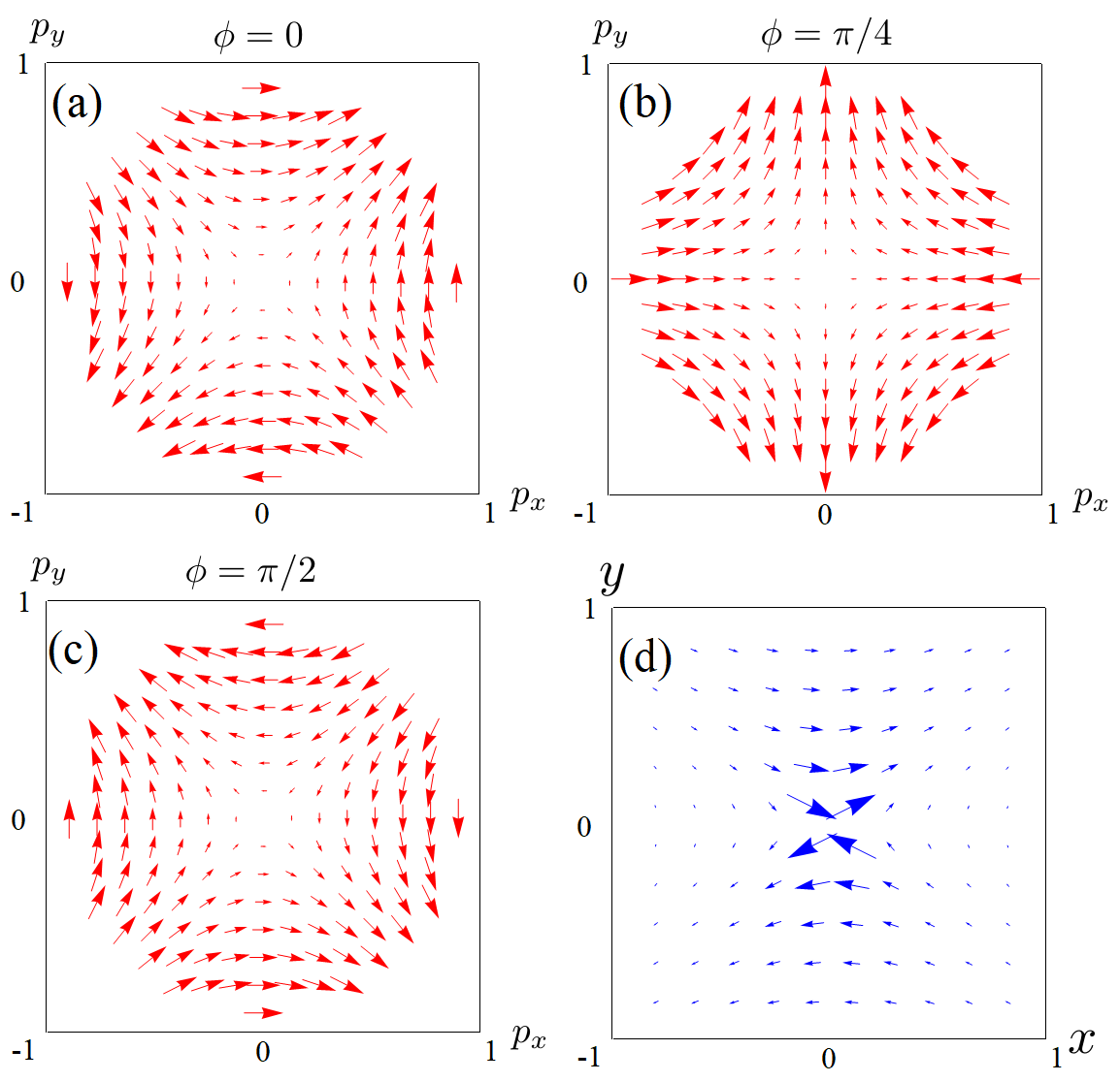
The above analysis in the small $\boldsymbol{p}$ reveals the structure of spin-orbit coupling (or pseudospin-orbit coupling if $\boldsymbol{\sigma}$ is not the real spin) arising from space-dependent tilt parameter $\boldsymbol{\zeta}$. When the $\boldsymbol{\zeta}$ that enters as an off-diagonal term mixing space and time is absent, as can be seen from Eq. (12), the $\omega^{i0}_{\mu}$ components of the spin-connection vanish from which it follows that the non-Abelian gauge fields in Eq. (16) vanish. When the $\boldsymbol{\zeta}$ term is introduced in tilted Dirac/Weyl systems and for whatever reason possess a non-trivial space dependence, the connections $\omega^{0i}_{\mu}$ (which multiply the matrices $\gamma_{0}\gamma_{i}$) become non-zero and generate the non-Abelian gauge structure in Eq. (16). Allowing the spatial components of the metric to depend on space (driven e.g. by strain), will generate the $\omega^{ij}_{\mu}$ components which are well known in the context of graphene and can only generate the $U(1)$ gauge structure, as they couple to $\gamma_{i}\gamma_{j}$ combination of Dirac matrices Vozmediano et al. 2010; De Juan et al. 2013.

When the length scale of applied fields are much larger than the spread of the wave packets, and the wave packets themselves are larger than the lattice constant, the semi-classical Boltzmann transport can be used to study the electron dynamics. In tilted Dirac/Weyl materials too, such a regime does exist and it is therefore appropriate to study the classical geodesics in a generic background metric (5) with space dependent $\boldsymbol{\zeta}$. This will allow us to develop a feeling at the classical level to the nature of the forces that correspond to the the non-Abelian gauge structure (16).

It is a well known textbook fact that gravitational forces around a rotating source that only slightly deform the metric $\eta^{\mu\nu}$ of the flat spacetime, can be effectively described by forces that resemble the electromagnetic forces. These effects go under the name of gravitomagnetic effects ⁶⁶ 6 See e.g. chapter 6 of the Ryder’s textbook Ryder 2009.. The effect of rotation goes into a weak off-diagonal element that mixes space and time. This feature is similar to our metric (5), except that (i) $\boldsymbol{\zeta}$ in our case is not necessarily weak and (ii) its functional dependence on space coordinates $(x,y)$ can in principle be anything. Therefore in this section we set out to understand the meaning of the space-dependent tilt parameter $\boldsymbol{\zeta}$ in the metric (5) of the tilted Dirac/Weyl materials. We will follow the textbook approach of Ryder and will start by writing down the geodesics equations in the background metric (5) in order to identify the structure of the new forces that arise from spatial variation of $\boldsymbol{\zeta}$ at the classical level. In the case of graphene where only the spatial components $g^{ij}$ of the metric are allowed to depend on space (due to strain field), it has been found that the curvature induced $U(1)$ forces, lead to spatial separation of the valley currents Stegmann and Szpak 2018.

Our classical treatment in this section, parallels the quantum treatment of section III as in both cases we consider the limit where a mass term is present that allows to approximate the Dirac hyperbola by a parabola. The geodesic equation is given by Ryder 2009

where $s$ is the proper time. In the non-relativistic (or in gravitational jargon the ”Newtonian”) limit, $s\approx t$ and $dx^{0}/ds\approx v_{F}$ and $dx^{i}/ds\approx v\ll v_{F}$. In this limit the acceleration $a^{i}=d^{2}x^{i}/dt^{2}$ will become,

Performing the summations over $k,m$ the separate components $i=1,2$ of the acceleration can be organized in powers of $v/v_{F}$ where $v$ is the band velocity near the bottom of conduction band and $v_{F}$ is the asymptotic velocity of Dirac electrons at large momenta. The leading order is

The first term in this equation is a gradient term. If $\zeta^{2}$ can be interpreted as negative of an ”electrostatic” potential, then the first term will correspond to the electric field arising from such term. There is however additional structure in the second term. When the variations of $\boldsymbol{\zeta}$ are purely transverse, the longitudinal derivative $\boldsymbol{\zeta}\cdot\boldsymbol{\partial}$ will vanish. If the spatial profile of $\zeta^{2}$ generated by external fields is localized around some origin ⁷⁷ 7 Perhaps this can be achieved by applying the electric field via a tip of thickness of several tens of nanometers., and decays away from it, will correspond to an inward acceleration if $m$ is positive (i.e. we for states near the bottom of conduction band). The gate voltage can be used to tune the chemical potential and therefore enables us to tune the Fermi level between the conduction and valence bands. This process will change the sign of $m$. Therefore if the above term is attractive for electrons it will be repulsive for holes, and vice versa.

The first order contribution is,

where $i=1,2$ correspond to $\bar{i}=2,1$, respectively. Note that $i$ is the free index of the left side and there is no sum over $i$ on the right side.

For the inversion symmetric tilted Dirac materials the two valleys have opposite $\boldsymbol{\zeta}$. The velocity independent terms, $\boldsymbol{a}_{(0)}$ in Eq. (29) are even in $\boldsymbol{\zeta}$. Therefore, they do not change upon $\boldsymbol{\zeta}\to-\boldsymbol{\zeta}$. Therefore these terms are the same in both valleys in such materials. The first order terms in Eq. (31) are odd in $\boldsymbol{\zeta}$. Therefore these can be attributed to the pseudo-forces in inversion symmetric system. Particularly, the third line in Eq. (31) is a Lorentz-type force provided $\boldsymbol{\zeta}$ can be imagined as the spatial part of a vector potential such that $\boldsymbol{\partial}\times\boldsymbol{\zeta}$ would correspond to a pseudo-magnetic field. Again by pseudo we mean that this field begin odd in $\boldsymbol{\zeta}$, changes sign in the other valley. The first line resembles a ”friction” force as the $i$’th component of the acceleration is proportional to $v^{i}$. Depending on the sign of the term in the parenthesis, this can be friction or anti-friction! In the later case, this term will cause an increase in the velocity, until the Newtonian regime ceases to be valid. In analogy with the first line, one can think of the second line as a kind of transverse friction” force which is then expected to enhance the shear viscosity when the interactions are turned on to form an electron liquid.

To develop a feeling for the classical dynamics in the spacetime (5), let us consider the special case where $\boldsymbol{\zeta}=(h(x),0)$ is varied only unidirectionally along the $\boldsymbol{\zeta}$ direction. We will further assume that $h(x)=\zeta_{0}\tanh(\frac{x}{\lambda})$. In this case for the zeroth order contribution we get,

and

and the first order contribution is

which for our step-like function becomes,

Note that in this section what we have calculated is the acceleration. To convert it to the force, one must note that it has to be multiplied by a mass term $m$. This term is positive for the states near the bottom of the conduction band. For those near the top of the valence band, this term (determining the parabola) is negative. Therefore the sign of the above forces can be reversed by e.g. gate doping and toggling the chemical potential between the valence to conduction bands. In this way, the sign of the force depends on the sign of charge carriers. Therefore the electric and magnetic forces emerging from the structure of the spacetime (5) reverse their signs by changing the ”charge” of the carriers. As such, these forces can be regarded as a natural generalizatioins of electric and magnetic forces that arise from the geometry of the spacetime itself. The external electric or magnetic fields are assumed to be absent here. Therefore in studying the effect of external electric and magnetic fields on the transport of electrons, one must in addition to external electric and magnetic fields worry about the forces that arise from the curved nature of spacetime (5).

For a fixed chemical potential corresponding to a given sign of the energy, the sign of $m$ is fixed. In that case, all the terms, including the term that resebles the Lorentz-force in the third line of Eq. (31) change sign. As such the classical Landau orbits for electrons in the two valleys have opposite directions. Therefore this term (when strong enough) can generate valley-polarized edge currents. So the curvature engineering can in principle generate valley Hall effect. Even if the material is not perfectly inversion symmetric, the symmetric part of it (for whith two valleys are related by $\boldsymbol{\zeta}\to-\boldsymbol{\zeta}$) is capable of generating valley polarized effects.

In this work we have investigated the effect of spatial dependence in the tilt parameter $\boldsymbol{\zeta}$ that determines the metric (5). The essential quantity is $\alpha_{i}^{j}$ defined under Eq. (12). At quantum level this quantity gives rise to non-Abelian gauge fields. The meaning of such gauge fields becomes clear in the non-relativistic limit pertinent the bottom of conduction or top of valence band states which corresponds to various forms of spin-orbit coupling. This agrees with recent proposal by Shitade and coworkers on geometric spin-orbit coupling  Shitade and Minamitani 2020. At the classical level, from geodesic equations one can infer various forms of forces that have no analogs in solid state systems with Galilean structure. The sign of these forces can be changed by toggling between conduction and valence bands via a gate voltage and therefore for opposite charge carriers they have opposite signs. This means that these forces are natural extensions of electric and magnetic forces to the geometry (5). In studying transport properties of such systems, these forces are also expected to play role in addition to the external electric and magnetic fields acting on the charge carriers.

It is worth to reiterate why unlike the strain induced pseudo-gauge forces in graphene, here we have a non-Abelian gauge structure. The reason is that strain appears in spatial components $g_{ij}$ while the space dependence of the tilt in TDCMs appears through the off-diagonal entries $g_{0\mu}$ that mix space and time coordinates. These two ways of modifying the $g_{\mu\nu}$ metric have two different physics. Therefore strain can be used as additional control parameter to generate a pseudo-magnetic field in addition to the spin-orbit interactions arising from the spatial variations of $g_{0\mu}$ entries of the metric in TDCMs. Indeed generation of spin-orbit couplings by spatial variation of $\boldsymbol{\zeta}$ seems quite plausible: In our previous work Farajollahpour et al. 2019 we have found that the displacement field couples to $\boldsymbol{\zeta}$ via Rashba spin-orbit coupling. Now here we have a reversed situation. If for whatever reason the tilt $\boldsymbol{\zeta}$ acquires a dependence on space coordinates $x^{i}$, one will have various spin-orbit couplings, including Rashba.

In terms of possible materials realizations, in 2D materials there are many possibilities. The most prominent example is the organic compound. Replacing the iodine (I, $\zeta<1$) by halogens, such as F ($\zeta>1$) an average control of F substitution correspond to a space dependent tilt Geilhufe et al. 2018. Even a random substitution of halogens can lead to randomness in the $\boldsymbol{\zeta}$ which seems to be an interesting element to randomize and worth investigation, particularly from the point of view of the spacetime structure. Or the interface between I-rich and F-rich compound based on this organic systems can mimic black-hole horizon. The transition between type-I and type-II Weyl fermions is signaled by an enhancement of the superconducting pairing Li et al. 2017. This transition corresponds to crossing a black-hole horizon ⁸⁸ 8 One has to be careful that the ”effective” description in terms of a metric is valid at length scales much larger than the atomic scales. As such, such solid state black-holes are escapable in the atomic scales Kedem et al. 2020. In $8Pmmn$ borophene structure a displacement field couples to $\boldsymbol{\zeta}$ and can in principle be used to imprint varous profiles of $\zeta_{i}(x,y)$ Farajollahpour et al. 2019. Furthermore, magnetic textures Liang and Ojanen 2019 can also generate space dependet tilt parameter $\boldsymbol{\zeta}(x^{i})$.

Therefore the tilted Dirac cone systems in two space dimensions are promising frameworks for generation of spin-orbit coupling (synthetic gauge fields). The effect of spacetime geometry is not limited to such synthetic forces. The quantum emission which is at the heart of solid-state spectroscopies will also be affected by the spacetime curvature Maxime J Jacquet 2020. This might require a careful examination of the linear response theory that links theoretical calculations within the Kubo formula with experiments Girvin and Yang 2019.

We wish to thank Ahmad Reza Moradpour and Armin Ghazi for fruitful discussions and Prof. Dr. Reza Mansouri for insightful discussions and encouragements to push the idea of solid-state spacetime structures. S.A.J. appreciates research deputy of Sharif University of Technology, Grant No. G960214 and Iran Science Elites Foundation (ISEF).

References

- Zee (2010) A. Zee, Quantum Field Theory in a Nutshell (Princeton University Press, 2010).
- Peskin and Schroeder (1995) M. E. Peskin and D. V. Schroeder, An Introduction To Quantum Field Theory (Avalon Publishing, 1995).
- Tajima et al. (2006) N. Tajima, S. Sugawara, M. Tamura, Y. Nishio, and K. Kajita, Journal of the Physical Society of Japan 75, 051010 (2006).
- Katayama et al. (2006) S. Katayama, A. Kobayashi, and Y. Suzumura, Journal of the Physical Society of Japan 75, 054705 (2006).
- Kobayashi et al. (2007) A. Kobayashi, S. Katayama, Y. Suzumura, and H. Fukuyama, Journal of the Physical Society of Japan 76, 034711 (2007).
- Tajima and Kajita (2009) N. Tajima and K. Kajita, Science and Technology of Advanced Materials 10, 024308 (2009).
- Kobayashi et al. (2009) A. Kobayashi, S. Katayama, and Y. Suzumura, Science and Technology of Advanced Materials 10, 024309 (2009).
- Isobe (2017) H. Isobe, in Theoretical Study on Correlation Effects in Topological Matter (Springer Singapore, 2017) pp. 63–81.
- Kajita et al. (2014) K. Kajita, Y. Nishio, N. Tajima, Y. Suzumura, and A. Kobayashi, Journal of the Physical Society of Japan 83, 072002 (2014).
- Tajima et al. (2013) N. Tajima, T. Yamauchi, T. Yamaguchi, M. Suda, Y. Kawasugi, H. M. Yamamoto, R. Kato, Y. Nishio, and K. Kajita, Phys. Rev. B 88, 075315 (2013).
- Morinari et al. (2009) T. Morinari, T. Himura, and T. Tohyama, Journal of the Physical Society of Japan 78, 023704 (2009).
- Sugawara et al. (2010) S. Sugawara, M. Tamura, N. Tajima, R. Kato, M. Sato, Y. Nishio, and K. Kajita, Journal of the Physical Society of Japan 79, 113704 (2010).
- Goerbig et al. (2008) M. O. Goerbig, J.-N. Fuchs, G. Montambaux, and F. Piéchon, Phys. Rev. B 78, 045415 (2008).
- Goerbig et al. (2009) M. O. Goerbig, J.-N. Fuchs, G. Montambaux, and F. Piéchon, 85, 57005 (2009).
- Sári et al. (2014) J. Sári, C. Tőke, and M. O. Goerbig, Phys. Rev. B 90, 155446 (2014).
- Hirata et al. (2011) M. Hirata, K. Ishikawa, K. Miyagawa, K. Kanoda, and M. Tamura, Phys. Rev. B 84, 125133 (2011).
- Hirata et al. (2017) M. Hirata, K. Ishikawa, G. Matsuno, A. Kobayashi, K. Miyagawa, M. Tamura, C. Berthier, and K. Kanoda, Science 358, 1403 (2017).
- Hirata et al. (2016) M. Hirata, K. Ishikawa, K. Miyagawa, M. Tamura, C. Berthier, D. Basko, A. Kobayashi, G. Matsuno, and K. Kanoda, Nature Communications 7 (2016).
- Geilhufe et al. (2018) R. M. Geilhufe, B. Commeau, and G. W. Fernando, physica status solidi (RRL) - Rapid Research Letters 12, 1800081 (2018).
- Tao and Tsymbal (2018) L. L. Tao and E. Y. Tsymbal, Phys. Rev. B 98, 121102 (2018).
- Chiu et al. (2017) C.-K. Chiu, Y.-H. Chan, X. Li, Y. Nohara, and A. P. Schnyder, Phys. Rev. B 95, 035151 (2017).
- Morinari et al. (2010) T. Morinari, E. Kaneshita, and T. Tohyama, Phys. Rev. Lett. 105, 037203 (2010).
- Varykhalov et al. (2017) A. Varykhalov, D. Marchenko, J. Sánchez-Barriga, E. Golias, O. Rader, and G. Bihlmayer, Phys. Rev. B 95, 245421 (2017).
- Imai et al. (2013) Y. Imai, F. Nabeshima, D. Nakamura, T. Katase, H. Hiramatsu, H. Hosono, and A. Maeda, Journal of the Physical Society of Japan 82, 043709 (2013).
- Lu et al. (2016) H.-Y. Lu, A. S. Cuamba, S.-Y. Lin, L. Hao, R. Wang, H. Li, Y. Zhao, and C. S. Ting, Phys. Rev. B 94, 195423 (2016).
- Zhou et al. (2014) X.-F. Zhou, X. Dong, A. R. Oganov, Q. Zhu, Y. Tian, and H.-T. Wang, Phys. Rev. Lett. 112, 085502 (2014).
- Lopez-Bezanilla and Littlewood (2016) A. Lopez-Bezanilla and P. B. Littlewood, Phys. Rev. B 93, 241405 (2016).
- Farajollahpour et al. (2019) T. Farajollahpour, Z. Faraei, and S. A. Jafari, Phys. Rev. B 99, 235150 (2019).
- Kawarabayashi et al. (2011) T. Kawarabayashi, Y. Hatsugai, T. Morimoto, and H. Aoki, Phys. Rev. B 83, 153414 (2011).
- Kishigi et al. (2011) K. Kishigi, K. Ueno, E. Miyamoto, and Y. Hasegawa, in Journal of Physics: Conference Series, Vol. 334 (IOP Publishing, 2011) p. 012047.
- Herrera and Naumis (2019) S. A. Herrera and G. G. Naumis, Phys. Rev. B 100, 195420 (2019).
- Proskurin et al. (2015) I. Proskurin, M. Ogata, and Y. Suzumura, Phys. Rev. B 91, 195413 (2015).
- Suzumura et al. (2014) Y. Suzumura, I. Proskurin, and M. Ogata, Journal of the Physical Society of Japan 83, 023701 (2014).
- Rostamzadeh et al. (2019) S. Rostamzadeh, I. Adagideli, and M. O. Goerbig, Phys. Rev. B 100, 075438 (2019).
- Verma et al. (2017) S. Verma, A. Mawrie, and T. K. Ghosh, Phys. Rev. B 96, 155418 (2017).
- Nishine et al. (2010) T. Nishine, A. Kobayashi, and Y. Suzumura, Journal of the Physical Society of Japan 79, 114715 (2010).
- Nishine et al. (2011) T. Nishine, A. Kobayashi, and Y. Suzumura, Journal of the Physical Society of Japan 80, 114713 (2011).
- Jalali-Mola and Jafari (2018a) Z. Jalali-Mola and S. A. Jafari, Phys. Rev. B 98, 195415 (2018a).
- Jalali-Mola and Jafari (2018b) Z. Jalali-Mola and S. A. Jafari, Phys. Rev. B 98, 235430 (2018b).
- Gao and Xiao (2018) Y. Gao and D. Xiao, Phys. Rev. B 98, 060402 (2018).
- Sinha (2019) D. Sinha, The European Physical Journal B 92 (2019).
- Sengupta et al. (2018) P. Sengupta, Y. Tan, E. Bellotti, and J. Shi, Journal of Physics: Condensed Matter 30, 435701 (2018).
- Isobe and Nagaosa (2012) H. Isobe and N. Nagaosa, Journal of the Physical Society of Japan 81, 113704 (2012).
- Yang et al. (2018) Z.-K. Yang, J.-R. Wang, and G.-Z. Liu, Phys. Rev. B 98, 195123 (2018).
- Xiao et al. (2017) H.-X. Xiao, J.-R. Wang, H.-T. Feng, P.-L. Yin, and H.-S. Zong, Phys. Rev. B 96, 155114 (2017).
- (46) D. Ohki, M. Hirata, T. Tani, K. Kanoda, and A. Kobayashi, arXiv preprint arXiv:1910.08999 .
- Faraei and Jafari (2019a) Z. Faraei and S. A. Jafari, Phys. Rev. B 100, 245436 (2019a).
- Faraei and Jafari (2019b) Z. Faraei and S. Jafari, arXiv preprint arXiv:1912.06355 (2019b).
- Li et al. (2017) D. Li, B. Rosenstein, B. Y. Shapiro, and I. Shapiro, Phys. Rev. B 95, 094513 (2017).
- Soluyanov et al. (2015) A. A. Soluyanov, D. Gresch, Z. Wang, Q. Wu, M. Troyer, X. Dai, and B. A. Bernevig, Nature 527, 495 (2015).
- Bruno et al. (2016) F. Y. Bruno, A. Tamai, Q. S. Wu, I. Cucchi, C. Barreteau, A. de la Torre, S. McKeown Walker, S. Riccò, Z. Wang, T. K. Kim, M. Hoesch, M. Shi, N. C. Plumb, E. Giannini, A. A. Soluyanov, and F. Baumberger, Phys. Rev. B 94, 121112 (2016).
- Wu et al. (2016a) Y. Wu, D. Mou, N. H. Jo, K. Sun, L. Huang, S. L. Bud’ko, P. C. Canfield, and A. Kaminski, Phys. Rev. B 94, 121113 (2016a).
- Wang et al. (2016) C. Wang, Y. Zhang, J. Huang, S. Nie, G. Liu, A. Liang, Y. Zhang, B. Shen, J. Liu, C. Hu, Y. Ding, D. Liu, Y. Hu, S. He, L. Zhao, L. Yu, J. Hu, J. Wei, Z. Mao, Y. Shi, X. Jia, F. Zhang, S. Zhang, F. Yang, Z. Wang, Q. Peng, H. Weng, X. Dai, Z. Fang, Z. Xu, C. Chen, and X. J. Zhou, Phys. Rev. B 94, 241119 (2016).
- Sun et al. (2015) Y. Sun, S.-C. Wu, M. N. Ali, C. Felser, and B. Yan, Phys. Rev. B 92, 161107 (2015).
- Deng et al. (2016) K. Deng, G. Wan, P. Deng, K. Zhang, S. Ding, E. Wang, M. Yan, H. Huang, H. Zhang, Z. Xu, J. Denlinger, A. Fedorov, H. Yang, W. Duan, H. Yao, Y. Wu, S. Fan, H. Zhang, X. Chen, and S. Zhou, Nature Physics 12, 1105 (2016).
- Jiang et al. (2017) J. Jiang, Z. Liu, Y. Sun, H. Yang, C. Rajamathi, Y. Qi, L. Yang, C. Chen, H. Peng, C.-C. Hwang, S. Sun, S.-K. Mo, I. Vobornik, J. Fujii, S. Parkin, C. Felser, B. Yan, and Y. Chen, Nature Communications 8 (2017).
- Huang et al. (2016a) L. Huang, T. M. McCormick, M. Ochi, Z. Zhao, M.-T. Suzuki, R. Arita, Y. Wu, D. Mou, H. Cao, J. Yan, N. Trivedi, and A. Kaminski, Nature Materials 15, 1155 (2016a).
- (58) N. Xu, Z. Wang, A. Weber, A. Magrez, P. Bugnon, H. Berger, C. Matt, J. Ma, B. Fu, B. Lv, et al., arXiv preprint arXiv:1604.02116 .
- (59) A. Liang, J. Huang, S. Nie, Y. Ding, Q. Gao, C. Hu, S. He, Y. Zhang, C. Wang, B. Shen, et al., arXiv preprint arXiv:1604.01706 .
- Wu et al. (2016b) Y. Wu, D. Mou, N. H. Jo, K. Sun, L. Huang, S. L. Bud’ko, P. C. Canfield, and A. Kaminski, Phys. Rev. B 94, 121113 (2016b).
- Huang et al. (2016b) H. Huang, S. Zhou, and W. Duan, Phys. Rev. B 94, 121117 (2016b).
- Zhang et al. (2017) K. Zhang, M. Yan, H. Zhang, H. Huang, M. Arita, Z. Sun, W. Duan, Y. Wu, and S. Zhou, Phys. Rev. B 96, 125102 (2017).
- Fei et al. (2017) F. Fei, X. Bo, R. Wang, B. Wu, J. Jiang, D. Fu, M. Gao, H. Zheng, Y. Chen, X. Wang, H. Bu, F. Song, X. Wan, B. Wang, and G. Wang, Phys. Rev. B 96, 041201 (2017).
- Fei et al. (2018) F. Fei, X. Bo, P. Wang, J. Ying, J. Li, K. Chen, Q. Dai, B. Chen, Z. Sun, M. Zhang, F. Qu, Y. Zhang, Q. Wang, X. Wang, L. Cao, H. Bu, F. Song, X. Wan, and B. Wang, Advanced Materials 30, 1801556 (2018).
- Noh et al. (2017) H.-J. Noh, J. Jeong, E.-J. Cho, K. Kim, B. I. Min, and B.-G. Park, Phys. Rev. Lett. 119, 016401 (2017).
- Yan et al. (2017) M. Yan, H. Huang, K. Zhang, E. Wang, W. Yao, K. Deng, G. Wan, H. Zhang, M. Arita, H. Yang, Z. Sun, H. Yao, Y. Wu, S. Fan, W. Duan, and S. Zhou, Nature Communications 8, 257 (2017).
- Kariyado and Ogata (2011) T. Kariyado and M. Ogata, Journal of the Physical Society of Japan 80, 083704 (2011).
- Khoury et al. (2019) J. F. Khoury, A. J. E. Rettie, M. A. Khan, N. J. Ghimire, I. Robredo, J. E. Pfluger, K. Pal, C. Wolverton, A. Bergara, J. S. Jiang, L. M. Schoop, M. G. Vergniory, J. F. Mitchell, D. Y. Chung, and M. G. Kanatzidis, Journal of the American Chemical Society 141, 19130 (2019).
- Trescher et al. (2015) M. Trescher, B. Sbierski, P. W. Brouwer, and E. J. Bergholtz, Phys. Rev. B 91, 115135 (2015).
- Trescher et al. (2017) M. Trescher, B. Sbierski, P. W. Brouwer, and E. J. Bergholtz, Phys. Rev. B 95, 045139 (2017).
- Tchoumakov et al. (2016) S. Tchoumakov, M. Civelli, and M. O. Goerbig, Phys. Rev. Lett. 117, 086402 (2016).
- Carbotte (2016) J. P. Carbotte, Phys. Rev. B 94, 165111 (2016).
- Sikkenk and Fritz (2017) T. S. Sikkenk and L. Fritz, Phys. Rev. B 96, 155121 (2017).
- Zyuzin and Tiwari (2016) A. A. Zyuzin and R. P. Tiwari, JETP Letters 103, 717 (2016).
- Arı et al. (2011) O. Arı, I. Dursun, and R. T. Senger, arXiv preprint arXiv:1105.0547 (2011).
- Volovik (2016) G. E. Volovik, JETP Letters 104, 645 (2016).
- Nissinen and Volovik (2017) J. Nissinen and G. E. Volovik, JETP Letters 105, 447 (2017).
- Martel and Poisson (2001) K. Martel and E. Poisson, American Journal of Physics 69, 476 (2001).
- Carrol (2003) S. Carrol, Spacetime and Geometry: An Introduction to General Relativity (Pearson, 2003).
- Iorio and Lambiase (2014) A. Iorio and G. Lambiase, Phys. Rev. D 90, 025006 (2014).
- Iorio (2013) A. Iorio, in Journal of Physics: Conference Series, Vol. 442 (IOP Publishing, 2013) p. 012056.
- Matsuo et al. (2011a) M. Matsuo, J. Ieda, E. Saitoh, and S. Maekawa, Phys. Rev. B 84, 104410 (2011a).
- Matsuo et al. (2011b) M. Matsuo, J. Ieda, E. Saitoh, and S. Maekawa, Phys. Rev. Lett. 106, 076601 (2011b).
- Jafari (2019) S. A. Jafari, Physical Review B 100 (2019), 10.1103/physrevb.100.045144.
- Jalali-Mola and Jafari (2019) Z. Jalali-Mola and S. A. Jafari, Phys. Rev. B 100, 075113 (2019).
- Liang and Ojanen (2019) L. Liang and T. Ojanen, Phys. Rev. Res. 1, 032006 (2019).
- Westström and Ojanen (2017) A. Westström and T. Ojanen, Phys. Rev. X 7, 041026 (2017).
- Arias et al. (2015) E. Arias, A. R. Hernández, and C. Lewenkopf, Phys. Rev. B 92, 245110 (2015).
- Ryder (2009) L. Ryder, Introduction to General Relativity (Cambridge University Press, 2009).
- Fließbach (2012) T. Fließbach, Allgemeine Relativitätstheorie, Vol. 3 (Springer, 2012).
- Arfken and Weber (1999) G. B. Arfken and H. J. Weber, “Mathematical methods for physicists,” (1999).
- Nakahara (2003) M. Nakahara, Geometry, topology and physics (CRC Press, 2003).
- Birrell and Davies (1984) N. D. Birrell and P. Davies, Quantum fields in curved space, 7 (Cambridge university press, 1984).
- Vozmediano et al. (2010) M. A. Vozmediano, M. Katsnelson, and F. Guinea, Physics Reports 496, 109 (2010).
- De Juan et al. (2013) F. De Juan, J. L. Manes, and M. A. Vozmediano, Physical Review B 87, 165131 (2013).
- Guinea et al. (2009) F. Guinea, B. Horovitz, and P. Le Doussal, Solid State Communications 149, 1140 (2009).
- Guinea et al. (2008) F. Guinea, B. Horovitz, and P. Le Doussal, Physical Review B 77, 205421 (2008).
- Shitade and Minamitani (2020) A. Shitade and E. Minamitani, arXiv preprint arXiv:2002.05371 (2020).
- Stegmann and Szpak (2018) T. Stegmann and N. Szpak, 2D Materials 6, 015024 (2018).
- Kedem et al. (2020) Y. Kedem, E. J. Bergholtz, and F. Wilczek, arXiv preprint arXiv:2001.02625 (2020).
- Maxime J Jacquet (2020) F. K. Maxime J Jacquet, arxiv:2001.05807 (2020).
- Girvin and Yang (2019) S. M. Girvin and K. Yang, Modern Condensed Matter Physics (Cambridge University Press, 2019).