Supplementary Material For: Interpretable Random Forests via Rule Extraction

The first step of SIRUS is to grow a random forest with a large number $M$ of trees based on the available sample $\mathscr{D}_{n}$. The critical feature of our approach to stabilize the forest structure is to restrict node splits to the $q$-empirical quantiles of the marginals $\smash{X^{(1)},\ldots,X^{(p)}}$, with typically $q=10$. This modification to Breiman’s original algorithm has a small impact on predictive accuracy, but is essential for stability, as it is extensively discussed in Section $3$ of the Supplementary Material. Next, the obtained forest is broken down in a large collection of rules in the following process. First, observe that each node of each tree of the resulting ensemble defines a hyperrectangle in the input space $\mathds{R}^{p}$. Such a node can therefore be turned into an elementary regression rule, by defining a piecewise constant estimate whose value only depends on whether the query point falls in the hyperrectangle or not. Formally, a (inner or terminal) node of the tree is represented by a path, say $\mathscr{P}$, which describes the sequence of splits to reach the node from the root of the tree. In the sequel, we denote by $\Pi$ the finite list of all possible paths, and insist that each path $\mathscr{P}\in\Pi$ defines a regression rule. Based on this principle, in the first step of the algorithm, both internal and external nodes are extracted from the trees of the random forest to generate a large collection of rules, typically $10^{4}$.

The second step of SIRUS is to select the relevant rules from this large collection. Despite the tree randomization in the forest construction, there are some redundancy in the extracted rules. Indeed those with a high frequency of appearance represent strong and robust patterns in the data, and are therefore good candidates to be included in a compact, stable, and predictive rule ensemble. This occurrence frequency is denoted by $\hat{p}_{M,n}(\mathscr{P})$ for each possible path $\mathscr{P}\in\Pi$. Then a threshold $p_{0}\in(0,1)$ is simply used to select the relevant rules, that is

$$\hat{\mathscr{P}}_{M,n,p_{0}}=\{\mathscr{P}\in\Pi:\hat{p}_{M,n}(\mathscr{P})>p_{0}\}.$$

The threshold $p_{0}$ is a tuning parameter, whose influence and optimal setting are discussed and illustrated later in the experiments (Figures 2 and 3). Optimal $p_{0}$ values essentially select rules made of one or two splits. Indeed, rules with a higher number of splits are more sensitive to data perturbation, and thus associated to smaller values of $\hat{p}_{M,n}(\mathscr{P})$. Therefore, SIRUS grows shallow trees to reduce the computational cost while leaving the rule selection untouched—see Section $3$ of the Supplementary Material. In a word, SIRUS uses the principle of randomized bagging, but aggregates the forest structure itself instead of predictions in order to stabilize the rule selection.

The rules associated with the set of distinct paths $\hat{\mathscr{P}}_{M,n,p_{0}}$ are dependent by definition of the path extraction mechanism. As an example, let us consider the $6$ rules extracted from a random tree of depth $2$. Since the tree structure is recursive, $2$ rules are made of one split and $4$ rules of two splits. Those $6$ rules are linearly dependent because their associated hyperrectangles overlap. Consequently, to properly settle a linear aggregation of the rules, the third step of SIRUS filters $\smash{\hat{\mathscr{P}}_{M,n,p_{0}}}$ with the following post-treatment procedure: if the rule induced by the path $\smash{\mathscr{P}\in\hat{\mathscr{P}}_{M,n,p_{0}}}$ is a linear combination of rules associated with paths with a higher frequency of appearance, then $\mathscr{P}$ is simply removed from $\smash{\hat{\mathscr{P}}_{M,n,p_{0}}}$. We refer to Section $4$ of the Supplementary Material for a detailed illustration of the post-treatment procedure on real data.

By following the previous steps, we finally obtain a small set of regression rules. As such, a rule $\hat{g}_{n,\mathscr{P}}$ associated with a path $\mathscr{P}$ is a piecewise constant estimate: if a query point x falls into the corresponding hyperrectangle $H_{\mathscr{P}}\subset\mathds{R}^{p}$, the rule returns the average of the $Y_{i}$’s for the training points $\textbf{X}_{i}$’s that belong to $H_{\mathscr{P}}$; symmetrically, if x falls outside of $H_{\mathscr{P}}$, the average of the $Y_{i}$’s for training points outside of $H_{\mathscr{P}}$ is returned. Next, a non-negative weight is assigned to each of the selected rule, in order to combine them into a single estimate of $m(\textbf{x})$. These weights are defined as the ridge regression solution, where each predictor is a rule $\hat{g}_{n,\mathscr{P}}$ for $\smash{\mathscr{P}\in\hat{\mathscr{P}}_{M,n,p_{0}}}$ and weights are constrained to be non-negative. Thus, the aggregated estimate $\hat{m}_{M,n,p_{0}}(\textbf{x})$ of $m(\textbf{x})$ computed in the fourth step of SIRUS has the form

$\displaystyle\hat{m}_{M,n,p_{0}}(\textbf{x})=\hat{\beta}_{0}+\sum_{\mathscr{P}\in\hat{\mathscr{P}}_{M,n,p_{0}}}\hat{\beta}_{n,\mathscr{P}}\hat{g}_{n,\mathscr{P}}(\textbf{x}),$

(2.1)

where $\hat{\beta}_{0}$ and $\hat{\beta}_{n,\mathscr{P}}$ are the solutions of the ridge regression problem. More precisely, denoting by $\smash{\boldsymbol{\hat{\beta}}_{n,p_{0}}}$ the column vector whose components are the coefficients $\smash{\hat{\beta}_{n,\mathscr{P}}}$ for $\smash{\mathscr{P}\in\hat{\mathscr{P}}_{M,n,p_{0}}}$, and letting $\mathbf{Y}=(Y_{1},\ldots,Y_{n})^{T}$ and $\boldsymbol{\Gamma}_{n,p_{0}}$ the matrix whose rows are the rule values $\hat{g}_{n,\mathscr{P}}(\textbf{X}_{i})$ for $i\in\{1,\ldots,n\}$, we have

	$\displaystyle(\boldsymbol{\hat{\beta}}_{n,p_{0}},\hat{\beta}_{0})=\underset{\boldsymbol{\beta}\geq 0,\beta_{0}}{\textrm{argmin}}\frac{1}{n}$	$\displaystyle||\mathbf{Y}-\beta_{0}\boldsymbol{1_{n}}-\boldsymbol{\Gamma}_{n,p_{0}}\boldsymbol{\beta}||_{2}^{2}$
		$\displaystyle+\lambda||\boldsymbol{\beta}||_{2}^{2},$

where $\boldsymbol{1_{n}}=(1,\ldots,1)^{T}$ is the $n$-vector with all components equal to $1$, and $\lambda$ is a positive parameter tuned by cross-validation that controls the penalization severity. The mininum is taken over $\beta_{0}\in\mathds{R}$ and all the vectors $\smash{\boldsymbol{\beta}=\{\beta_{1},\ldots,\beta_{c_{n}}\}\in\mathds{R}_{+}^{c_{n}}}$ where $\smash{c_{n}=|\hat{\mathscr{P}}_{M,n,p_{0}}|}$ is the number of selected rules. Besides, notice that the rule format with an else clause differs from the standard format in the rule learning literature. This modification provides good properties of stability and modularity (investigation of the rules one by one (Murdoch et al., 2019)) to SIRUS—see Section $5$ of the Supplementary Material.

This linear rule aggregation is a critical step and deserves additional comments. Indeed, in RuleFit, the rules are also extracted from a tree ensemble, but aggregated using the Lasso. However, the extracted rules are strongly correlated by construction, and the Lasso selection is known to be highly unstable in such correlated setting. This is the main reason of the instability of RuleFit, as the experiments will show. On the other hand, the sparsity of SIRUS is controlled by the parameter $p_{0}$, and the ridge regression enables a stable aggregation of the rules. Furthermore, the constraint $\boldsymbol{\beta}\geq 0$ is added to ensure that all coefficients are non-negative, as in Node harvest (Meinshausen, 2010). Also because of the rule correlation, an unconstrained regression would lead to negative values for some of the coefficients $\smash{\hat{\beta}_{n,\mathscr{P}}}$, and such behavior drastically undermines the interpretability of the algorithm.

As stated in the introduction, despite the lack of a precise definition of interpretable models, there are three minimum requirements to be taken into account: simplicity, stability, and predictivity. These notions need to be formally defined and quantified to enable comparison between algorithms. Simplicity refers to the model complexity, in particular the number of operations involved in the prediction mechanism. In the case of rule algorithms, a measure of simplicity is naturally given by the number of rules. Intuitively, a rule algorithm is stable when two independent estimations based on two independent samples return similar lists of rules. Formally, let $\smash{\hat{\mathscr{P}}_{M,n,p_{0}}^{\prime}}$ be the list of rules output by SIRUS fit on an independent sample $\mathscr{D}_{n}^{\prime}$. Then the proportion of rules shared by $\smash{\hat{\mathscr{P}}_{M,n,p_{0}}}$ and $\smash{\hat{\mathscr{P}}_{M,n,p_{0}}^{\prime}}$ gives a stability measure. Such a metric is known as the Dice-Sorensen index, and is often used to assess variable selection procedures (Chao et al., 2006; Zucknick et al., 2008; Boulesteix and Slawski, 2009; He and Yu, 2010; Alelyani et al., 2011). In our case, the Dice-Sorensen index is then defined as

$\displaystyle\hat{S}_{M,n,p_{0}}=\frac{2\big|\hat{\mathscr{P}}_{M,n,p_{0}}\cap\hat{\mathscr{P}}_{M,n,p_{0}}^{\prime}\big|}{\big|\hat{\mathscr{P}}_{M,n,p_{0}}\big|+\big|\hat{\mathscr{P}}_{M,n,p_{0}}^{\prime}\big|}.$

However, in practice one rarely has access to an additional sample $\mathscr{D}_{n}^{\prime}$. Therefore, to circumvent this problem, we use a $10$-fold cross-validation to simulate data perturbation. The stability metric is thus empirically defined as the average proportion of rules shared by two models of two distinct folds of the cross-validation. A stability of $1$ means that the exact same list of rules is selected over the $10$ folds, whereas a stability of $0$ means that all rules are distinct between any $2$ folds. For predictivity in regression problems, the proportion of unexplained variance is a natural measure of the prediction error. The estimation is performed by $10$-fold cross-validation.

Our algorithm is illustrated on the “LA Ozone” dataset from Friedman et al., 2001, which records the level of atmospheric ozone concentration from eight daily meteorological measurements made in Los Angeles in 1976: wind speed (“wind”), humidity (“humidity”), temperature (“temp”), inversion base height (“ibh”), daggot pressure gradient (“dpg”), inversion base temperature (“ibt”), visibility (“vis”), and day of the year (“doy”). The response “Ozone” is the log of the daily maximum of ozone concentration. The list of rules output for this dataset is presented in Table 1. The column “Frequency” refers to $\hat{p}_{M,n}(\mathscr{P})$, the occurrence frequency of each rule in the forest, used for rule selection. It enables to grasp how weather conditions impact the ozone concentration. In particular, a temperature larger than $65$°F or a high inversion base temperature result in high ozone concentrations. The third rule tells us that the interaction of a high temperature with a visibility lower than $150$ miles generates even higher levels of ozone concentration. Interestingly, according to the ninth rule, especially low ozone concentrations are reached when a low temperature and and a low inversion base temperature are combined. Recall that to generate a prediction for a given query point x, for each rule the corresponding ozone concentration is retrieved depending on whether x satisfies the rule conditions. Then all rule outputs for x are multiplied by their associated weight and added together. One can observe that rule importances and weights are not related. For example, the third rule has a higher weight than the most two important ones. It is clear that rule $3$ has multiple constraints and is therefore more sensitive to data perturbation—hence a smaller frequency of appearance in the forest. On the other hand, its associated variance decrease in CART is more important than for the first two rules, leading to a higher weight in the linear combination. Since rules $5$ and $6$ are strongly correlated, their weights are diluted.

SIRUS has only one hyperparameter which requires fine tuning: the threshold $p_{0}$ to control the model size by selecting the most frequent rules in the forest. First, the range of possible values of $p_{0}$ is set so that the model size varies between $1$ and $25$ rules. This arbitrary upper bound is a safeguard to avoid long and complex list of rules that are difficult to interpret. In practice, this limit of $25$ rules is rarely hit, since the following tuning of $p_{0}$ naturally leads to compact rule lists. Thus, $p_{0}$ is tuned within that range by cross-validation to maximize both stability and predictivity. To find a tradeoff between these two properties, we follow a standard bi-objective optimization procedure as illustrated in Figure 5, and described in Section $2$ of the Supplementary Material: $p_{0}$ is chosen to be as close as possible to the ideal case of $0$ unexplained variance and $90\%$ stability. This tuning procedure is computationally fast: the cost of about $10$ fits of SIRUS. For a robust estimation of $p_{0}$, the cross-validation is repeated $10$ times and the median $p_{0}$ value is selected.

Besides, the optimal number of trees $M$ is set automatically by SIRUS: as stability, predictivity, and computation time increase with the number of trees, no fine tuning is required for $M$. Thus, a stopping criterion is designed to grow the minimum number of trees which enforces that stability and predictivity are greater than $95\%$ of their maximum values (reached when $M\rightarrow\infty$)—see Section $7$ of the Supplementary Material for a detailed definition of this criterion. Finally, we use the standard settings of random forests (well-known for their excellent performance, in particular mtry is $\lfloor p/3\rfloor$ and at least $2$), and set $q=10$ quantiles, while categorical variables are handled as natively defined in trees.

We compare SIRUS with its two main competitors RuleFit (with rule predictors only) and Node harvest. For predictive accuracy, we ran random forests and (pruned) CART to provide the baseline. Only to compute stability metrics, data is binned using $10$ quantiles to fit Rulefit and Node harvest. Our R/C++ package sirus (available from CRAN) is adapted from ranger, a fast random forests implementation (Wright and Ziegler, 2017). We also use available R implementations pre (Fokkema, 2017, RuleFit) and nodeharvest (Meinshausen, 2015). While the predictive accuracy of SIRUS is comparable to Node harvest and slightly below RuleFit, the stability is considerably improved with much smaller rule lists. Experimental results are gathered in Table 2a for model sizes, Table 2b for stability, and Table 3 for predictive accuracy. All results are averaged over $10$ repetitions of the cross-validation procedure. Since standard deviations are negligible, they are not displayed to increase readability. Besides, in the last column of Table 3, $p_{0}$ is set to increase the number of rules in SIRUS to reach RuleFit and Node harvest model size (about $50$ rules): predictivity is then as good as RuleFit. Finally, the column “SIRUS sparse” of Tables 2 and 3 shows the excellent behavior of SIRUS in a sparse setting: for each dataset, $3$ randomly permuted copies of each variable are added to the data, leaving SIRUS performance almost untouched.

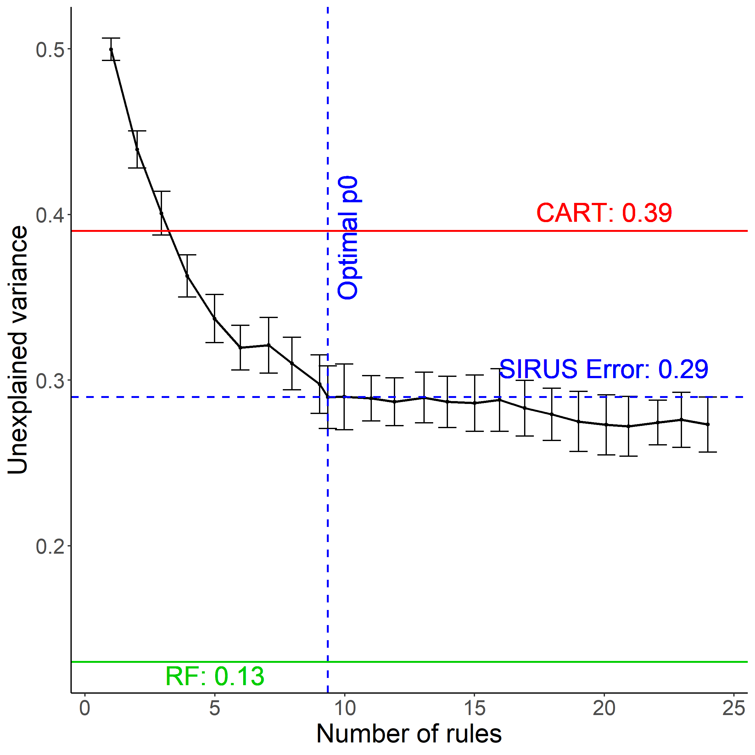
To illustrate the typical behavior of our method, we comment the results for two specific datasets: “Diabetes” (Efron et al., 2004) and “Machine” (Dua and Graff, 2017). The “Diabetes” data contains $n=442$ diabetic patients and the response of interest $Y$ is a measure of disease progression over one year. A total of $10$ variables are collected for each patient: age, sex, body mass index, average blood pressure, and six blood serum measurements $s1,s2,\ldots,s6$. For this dataset, SIRUS is as predictive as a random forest, with only $12$ rules when the forest performs about $10^{4}$ operations: the unexplained variance is $0.56$ for SIRUS and $0.55$ for random forest. Notice that CART performs considerably worse with $0.67$ unexplained variance. For the second dataset, “Machine”, the output $Y$ of interest is the CPU performance of computer hardware. For $n=209$ machines, $6$ variables are collected about the machine characteristics. For this dataset, SIRUS, RuleFit, and Node harvest have a similar predictivity, in-between CART and random forests. Our algorithm achieves such performance with a readable list of only $9$ rules stable at $86\%$, while RuleFit and Node harvest incorporate respectively $44$ and $42$ rules with stability levels of $23\%$ and $29\%$. Stability and predictivity are represented as $p_{0}$ varies for “Diabetes” and “Machine” datasets in Figures 2 and 3, respectively.

The first step of the proof is to show that the post-treated path extraction from the forest is consistent, i.e., in probability

$\displaystyle\lim_{n\to\infty}\mathds{P}(\hat{\mathscr{P}}_{M_{n},n,p_{0}}=\mathscr{P}^{\star}_{p_{0}})=1.$

(1.1)

Using the continuous mapping theorem, it is easy to see that this result is a consequence of the consistency of $\hat{p}_{M,n}(\mathscr{P})$, i.e.,

$$\lim\limits_{n\to\infty}\hat{p}_{M_{n},n}(\mathscr{P})=p^{\star}(\mathscr{P})\quad\textrm{in probability.}$$

Since the output $Y$ is bounded (by Assumption (A2)), the consistency of $\hat{p}_{M,n}(\mathscr{P})$ can be easily adapted from Theorem 1 of Bénard et al., 2021 using Assumptions (A1) and (A2). Finally, the result still holds for the post-treated rule set because the post-treatment is a deterministic procedure.

Recall that the estimate $(\boldsymbol{\hat{\beta}}_{n,p_{0}},\hat{\beta}_{0})$ is defined as

$\displaystyle(\boldsymbol{\hat{\beta}}_{n,p_{0}},\hat{\beta}_{0})=\underset{\boldsymbol{\beta}\geq 0,\beta_{0}}{\textrm{argmin }}\ell_{n}(\boldsymbol{\beta},\beta_{0}),$

(1.2)

where $\ell_{n}(\boldsymbol{\beta},\beta_{0})=\frac{1}{n}||\mathbf{Y}-\beta_{0}\boldsymbol{1_{n}}-\boldsymbol{\Gamma}_{n,p_{0}}\boldsymbol{\beta}||_{2}^{2}+\lambda||\boldsymbol{\beta}||_{2}^{2}.$ The dimension of $\beta$ is stochastic since it is equal to the number of extracted rules. To get rid of this technical issue in the following of the proof, we rewrite $\ell_{n}(\boldsymbol{\beta},\beta_{0})$ to have $\boldsymbol{\beta}$ a parameter of fixed dimension $|\Pi|$, the total number of possible rules:

$\displaystyle\ell_{n}(\boldsymbol{\beta},\beta_{0})=\frac{1}{n}\sum_{i=1}^{n}\big(Y_{i}-\beta_{0}-\sum_{\mathscr{P}\in\Pi}\beta_{\mathscr{P}}g_{n,\mathscr{P}}(\textbf{X}_{i})\mathds{1}_{\mathscr{P}\in\hat{\mathscr{P}}_{M_{n},n,p_{0}}}\big)^{2}+\lambda||\boldsymbol{\beta}||_{2}^{2}.$

By the law of large numbers and the previous result (1.1), we have in probability

$\displaystyle\lim\limits_{n\to\infty}\ell_{n}(\boldsymbol{\beta},\beta_{0})=$

$\displaystyle\mathbb{E}\big[\big(Y-\beta_{0}-\sum_{\mathscr{P}\in\mathscr{P}^{\star}_{p_{0}}}\beta_{\mathscr{P}}g_{\mathscr{P}}^{\star}(\textbf{X})\big)^{2}\big]+\lambda||\boldsymbol{\beta}||_{2}^{2}\mathrel{{\mathop{=}\limits}}\ell^{\star}(\boldsymbol{\beta},\beta_{0}),$

where $g_{\mathscr{P}}^{\star}$ is the theoretical rule based on the path $\mathscr{P}$ and the theoretical quantiles. Since $Y$ is bounded, it is easy to see that each component of $\boldsymbol{\hat{\beta}}_{n,p_{0}}$ is bounded from the following inequalities:

$\displaystyle\lambda||\boldsymbol{\hat{\beta}}_{n,p_{0}}||_{2}^{2}\leq\ell_{n}(\boldsymbol{\hat{\beta}}_{n,p_{0}},\hat{\beta}_{0})\leq\ell_{n}(\boldsymbol{0},0)\leq\frac{||Y||_{2}^{2}}{n}\leq\underset{i}{\max}\hskip 2.84526ptY_{i}^{2}.$

Consequently, the optimization problem (1.2) can be equivalently written with $(\boldsymbol{\beta},\beta_{0})$ constrained to belong to a compact and convex set $K$. Since $\ell_{n}$ is convex and converges pointwise to $\ell^{\star}$ according to (1), the uniform convergence over the compact set $K$ also holds, i.e., in probability

$\displaystyle\lim\limits_{n\to\infty}\underset{(\boldsymbol{\beta},\beta_{0})\in K}{\sup}|\ell_{n}(\boldsymbol{\beta},\beta_{0})-\ell^{\star}(\boldsymbol{\beta},\beta_{0})|=0.$

(1.3)

Additionnally, since $\ell^{\star}$ is a quadratic convex function and the constraint domain $K$ is convex, $\ell^{\star}$ has a unique minimum that we denote $\boldsymbol{\beta}^{\star}_{p_{0},\lambda}$. Finally, since the maximum of $\ell^{\star}$ is unique and $\ell_{n}$ uniformly converges to $\ell^{\star}$, we can apply theorem $5.7$ from Van der Vaart, 2000 to deduce that $(\boldsymbol{\hat{\beta}}_{n,p_{0}},\hat{\beta}_{0})$ is a consistent estimate of $\boldsymbol{\beta}^{\star}_{p_{0},\lambda}$. We can conclude that, in probability,

$\displaystyle\lim\limits_{n\to\infty}\mathds{P}\big(\hat{\mathscr{P}}_{M_{n},n,p_{0},\lambda}=\{\mathscr{P}\in\mathscr{P}^{\star}_{p_{0}}:\beta^{\star}_{\mathscr{P},p_{0},\lambda}>0\}\big)=1,$

and the final stability result follows from the continuous mapping theorem. ∎

SIRUS algorithm has several steps in its construction phase. We derive the computational complexity of each of them. Recall that $M$ is the number of trees, $p$ the number of input variables, and $n$ the sample size.

1. 1.

   Forest growing: $O(Mpnlog(n))$

   The forest growing is the most expensive step of SIRUS. The average computational complexity of a standard forest fit is $O(Mpnlog(n)^{2})$ (Louppe, 2014). Since the depth of trees is fixed in SIRUS—see Section $3$, it reduces to $O(Mpnlog(n))$.

   A standard forest is grown so that its accuracy cannot be significantly improved with additional trees, which typically results in about $500$ trees. In SIRUS, the stopping criterion of the number of trees enforces that $95\%$ of the rules are identical over multiple runs with the same dataset (see Section 7). This is critical to have the forest structure converged and stabilize the final rule list. This leads to forests with a large number of trees, typically $10$ times the number for standard forests. On the other hand, shallow trees are grown and the computational complexity is proportional to the tree depth, which is about $log(n)$ for fully grown forests.

   Overall, the modified forest used in SIRUS is about the same computational cost as a standard forest, and has a slightly better computational complexity thanks to the fixed tree depth.

2. 2.

   Rule extraction: $O(M)$

   Extracting the rules in a tree requires a number of operations proportional to the number of nodes, i.e. $O(1)$ since tree depth is fixed. With the appropriate data structure (a map), updating the forest count of the number of occurrences of the rules of a tree is also $O(1)$. Overall, the rule extraction is proportional to the number of trees in the forest, i.e., $O(M)$.

3. 3.

   Rule post-treatment: $O(1)$

   The post-treatment algorithm is only based on the rules and not on the sample. Since the number of extracted rules is bounded by a fixed limit of $25$, this step has a computational complexity of $O(1)$.

4. 4.

   Rule aggregation: $O(n)$

   Efficient algorithms (Friedman et al., 2010) enable to fit a ridge regression and find the optimal penalization $\lambda$ with a linear complexity in the sample size $n$. In SIRUS, the predictors are the rules, whose number is upper bounded by $25$, and then the complexity of the rule aggregation is independent of $p$. Therefore the computational complexity of this step is $O(n)$.

Overall, the computational complexity of SIRUS is $O(Mpnlog(n))$, which is slightly better than standard random forests thanks to the use of shallow trees. Because of the large number of trees and the final ridge regression, the computational cost of SIRUS is comparable to standard forests in practice.

In both RuleFit and Node harvest, the first two steps of the procedure are also to grow a tree ensemble with limited tree depth and extract all possible rules. The complexity of this first phase is then similar to SIRUS: $O(Mpnlog(n))$. However, in the last step of the linear rule aggregation, all rules are combined in a sparse linear model, which is of linear complexity with $n$, but grows at faster rate than linear with the number of rules, i.e., the number of trees $M$ (Friedman et al., 2010).

As the tree ensemble growing is the computational costly step, SIRUS, RuleFit and Node harvest have a very comparable complexity. On one hand, SIRUS requires to grow more trees than its competitors. On the other hand, the final linear rule aggregation is done with few predictors in SIRUS, while it includes thousands of rules in RuleFit and Node harvest, which has a complexity faster than linear with $M$.

The only parameter of SIRUS which requires fine tuning is $p_{0}$, which controls model sparsity. The optimal value is estimated by $10$-fold cross validation using a standard bi-objective optimization procedure to maximize both stability and predictivity. For a fine grid of $p_{0}$ values, the unexplained variance and stability metric are computed for the associated SIRUS model through a cross-validation. Recall that the bounds of the $p_{0}$ grid are set to get the model size between $1$ and $25$ rules. Next, we obtain a Pareto front, as illustrated in Figure 5, where each point corresponds to a $p_{0}$ value of the tuning grid. To find the optimal $p_{0}$, we compute the euclidean distance between each point and the ideal point of $0$ unexplained variance and $90\%$ stability. Notice that this ideal point is chosen for its empirical efficiency: the unexplained variance can be arbitrary close to $0$ depending on the data, whereas we do not observe a stability (with respect to data perturbation) higher than $90\%$ accross many datasets. Finally, the optimal $p_{0}$ is the one minimizing the euclidean distance distance to the ideal point. Thus, the two objectives, stability and predictivity, are equally weighted. For a robust estimation of $p_{0}$, the cross-validation is repeated $10$ times and the median $p_{0}$ value is selected.

The optimal $p_{0}$ value is estimated by a $10$-fold cross validation. The costly computational step of SIRUS is the forest growing. However, this step has to be done only once per fold. Then, $p_{0}$ can vary along a fine grid to extract more or less rules from each forest, and thus, get the accuracy associated to each $p_{0}$ at a total cost of about $10$ SIRUS fits.

In a typical setting where the number of predictors is $p=100$, limiting cut values to the $10$-quantiles splits the input space in a fine grid of $10^{100}$ hyperrectangles. Therefore, restricting cuts to quantiles still leaves a high flexibility to the forest and enables to identify local patterns (it is still true in small dimension). To illustrate this, we run the following experiment: for each of the $8$ datasets, we compute the unexplained variance of respectively the standard forest and the forest where cuts are limited to the $10$-quantiles. Results are presented in Table 4, and we see that there is almost no decrease of accuracy except for one dataset. Besides, notice that setting $q=n$ is equivalent as using original forests.

On the other hand, such discretization is critical for the stability of the rule selection. Recall that the importance of each rule $\hat{p}_{M,n}(\mathscr{P})$ is defined as the proportion of trees which contain its associated path $\mathscr{P}$, and that the rule selection is based on $\hat{p}_{M,n}(\mathscr{P})>p_{0}$. In the forest growing, data is bootstrapped prior to the construction of each tree. Without the quantile discretization, this data perturbation results in small variation between the cut values across different nodes, and then the dilution of $\hat{p}_{M,n}(\mathscr{P})$ between highly similar rules. Thus, the rule selection procedure becomes inefficient. More formally, $\hat{p}_{M,n}(\mathscr{P})$ is defined by

$$\hat{p}_{M,n}(\mathscr{P})=\frac{1}{M}\sum_{\ell=1}^{M}\mathds{1}_{\mathscr{P}\in T(\Theta_{\ell},\mathscr{D}_{n})},$$

where $T(\Theta_{\ell},\mathscr{D}_{n})$ is the list of paths extracted from the $\ell$-th tree of the forest. The expected value of the importance of a given rule is

$\displaystyle\mathbb{E}[\hat{p}_{M,n}(\mathscr{P})]=\frac{1}{M}\sum_{\ell=1}^{M}\mathbb{E}[\mathds{1}_{\mathscr{P}\in T(\Theta_{\ell},\mathscr{D}_{n})}]=\mathds{P}(\mathscr{P}\in T(\Theta,\mathscr{D}_{n})).$

Without the discretization, $T(\Theta,\mathscr{D}_{n})$ is a random set that takes value in an uncountable space, and consequently

$\displaystyle\mathbb{E}[\hat{p}_{M,n}(\mathscr{P})]=\mathds{P}(\mathscr{P}\in T(\Theta_{\ell},\mathscr{D}_{n}))=0,$

and all rules are equally not important in average. In practice, since $\mathscr{D}_{n}$ is of finite size and the random forest cuts at mid distance between two points, it is still possible to compute $\hat{p}_{M,n}(\mathscr{P})$ and select rules for a given dataset. However, such procedure is highly unstable with respect to data perturbation since we have $\mathbb{E}[\hat{p}_{M,n}(\mathscr{P})]=0$ for all possible paths.

When SIRUS is fit using fully grown trees, the final set of rules $\hat{\mathscr{P}}_{M,n,p_{0}}$ contains almost exclusively rules made of one or two splits, and very rarely of three splits. Although this may appear surprising at first glance, this phenomenon is in fact expected. Indeed, rules made of multiple splits are extracted from deeper tree levels and are thus more sensitive to data perturbation by construction. This results in much smaller values of $\hat{p}_{M,n}(\mathscr{P})$ for rules with a high number of splits, and then deletion from the final set of path through the threshold $p_{0}$: $\smash{\hat{\mathscr{P}}_{M,n,p_{0}}=\{\mathscr{P}\in\Pi:\hat{p}_{M,n}(\mathscr{P})>p_{0}\}}$. To illustrate this, let us consider the following typical example with $p=100$ input variables and $q=10$ quantiles. There are $2qp=2\times 100\times 10=2\times 10^{3}$ distinct rules of one split, about $(2qp)^{2}\approx 10^{6}$ distinct rules of two splits, and about $(2qp)^{3}\approx 10^{10}$ distinct rules of three splits. Using only rules of one split is too restrictive since it generates a small model class (a thousand rules for $100$ input variables) and does not handle variable interactions. On the other hand, rules of two splits are numerous (a million) and thus provide a large flexibility to SIRUS. More importantly, since there are $10$ billion rules of three splits, a stable selection of a few of them is clearly an impossible task, and such complex rules are naturally discarded by SIRUS.

In SIRUS, tree depth is set to $2$ to reduce the computational cost while leaving the output list of rules untouched as previously explained. We augment the experiments of Section $3$ of the article with an additional column in Table 3: “SIRUS $50$ rules & d$=3$”. Recall that, in the column “SIRUS $50$ rules”, $p_{0}$ is set manually to extract $100$ rules from the forest leading to final lists of about $50$ rules (similar size as RuleFit and Node harvest models), an improved accuracy (reaching RuleFit performance), while stability drops to around $50\%$ ($70-80\%$ when $p_{0}$ is tuned). In the last column, tree depth is set to $3$ with the same augmented model size. We observe no accuracy improvement over a tree depth of $2$.

This analysis of tree depth is not new. Indeed, both RuleFit (Friedman and Popescu, 2008) and Node harvest (Meinshausen, 2010) articles discuss the optimal tree depth for the rule extraction from a tree ensemble in their experiments. They both conclude that the optimal depth is $2$. Hence, the same hard limit of $2$ is used in Node harvest. RuleFit is slightly less restrictive: for each tree, its depth is randomly sampled with an exponential distribution concentrated on $2$, but allowing few trees of depth $1$, $3$ and $4$. We insist that they both reach such conclusion without considering stability issues, but only focusing on accuracy.

References

- Alelyani et al., (2011) Alelyani, S., Zhao, Z., and Liu, H. (2011). A dilemma in assessing stability of feature selection algorithms. In 13th IEEE International Conference on High Performance Computing & Communication, pages 701–707, Piscataway. IEEE.
- Bénard et al., (2021) Bénard, C., Biau, G., Da Veiga, S., and Scornet, E. (2021). Sirus: Stable and interpretable rule set for classification. Electronic Journal of Statistics, 15:427–505.
- Boulesteix and Slawski, (2009) Boulesteix, A.-L. and Slawski, M. (2009). Stability and aggregation of ranked gene lists. Briefings in Bioinformatics, 10:556–568.
- (4) Breiman, L. (2001a). Random forests. Machine Learning, 45:5–32.
- (5) Breiman, L. (2001b). Statistical modeling: The two cultures (with comments and a rejoinder by the author). Statistical Science, 16:199–231.
- Breiman et al., (1984) Breiman, L., Friedman, J., Olshen, R., and Stone, C. (1984). Classification and Regression Trees. Chapman & Hall/CRC, Boca Raton.
- Chao et al., (2006) Chao, A., Chazdon, R., Colwell, R., and Shen, T.-J. (2006). Abundance-based similarity indices and their estimation when there are unseen species in samples. Biometrics, 62:361–371.
- Clark and Niblett, (1989) Clark, P. and Niblett, T. (1989). The CN2 induction algorithm. Machine Learning, 3:261–283.
- Cohen, (1995) Cohen, W. (1995). Fast effective rule induction. In Proceedings of the 12th International Conference on Machine Learning, pages 115–123, San Francisco. Morgan Kaufmann Publishers Inc.
- Cohen and Singer, (1999) Cohen, W. and Singer, Y. (1999). A simple, fast, and effective rule learner. In Proceedings of the 16th National Conference on Artificial Intelligence and 11th Conference on Innovative Applications of Artificial Intelligence, pages 335–342, Palo Alto. AAAI Press.
- Dembczyński et al., (2010) Dembczyński, K., Kotłowski, W., and Słowiński, R. (2010). ENDER: A statistical framework for boosting decision rules. Data Mining and Knowledge Discovery, 21:52–90.
- Dua and Graff, (2017) Dua, D. and Graff, C. (2017). UCI machine learning repository.
- Efron et al., (2004) Efron, B., Hastie, T., Johnstone, I., and Tibshirani, R. (2004). Least angle regression. The Annals of statistics, 32:407–499.
- Fokkema, (2017) Fokkema, M. (2017). PRE: An R package for fitting prediction rule ensembles. arXiv:1707.07149.
- Frank and Witten, (1998) Frank, E. and Witten, I. H. (1998). Generating accurate rule sets without global optimization. In Proceedings of the 15th International Conference on Machine Learning, pages 144–151, San Francisco. Morgan Kaufmann Publishers Inc.
- Friedman et al., (2001) Friedman, J., Hastie, T., and Tibshirani, R. (2001). The Elements of Statistical Learning, volume 1. Springer, New York.
- Friedman et al., (2010) Friedman, J., Hastie, T., and Tibshirani, R. (2010). Regularization paths for generalized linear models via coordinate descent. Journal of statistical software, 33:1.
- Friedman and Popescu, (2003) Friedman, J. and Popescu, B. (2003). Importance sampled learning ensembles. Journal of Machine Learning Research, 94305:1–32.
- Friedman and Popescu, (2008) Friedman, J. and Popescu, B. (2008). Predictive learning via rule ensembles. The Annals of Applied Statistics, 2:916–954.
- Fürnkranz and Widmer, (1994) Fürnkranz, J. and Widmer, G. (1994). Incremental reduced error pruning. In Proceedings of the 11th International Conference on Machine Learning, pages 70–77, San Francisco. Morgan Kaufmann Publishers Inc.
- He and Yu, (2010) He, Z. and Yu, W. (2010). Stable feature selection for biomarker discovery. Computational Biology and Chemistry, 34:215–225.
- Letham et al., (2015) Letham, B., Rudin, C., McCormick, T., and Madigan, D. (2015). Interpretable classifiers using rules and Bayesian analysis: Building a better stroke prediction model. The Annals of Applied Statistics, 9:1350–1371.
- Lipton, (2016) Lipton, Z. (2016). The mythos of model interpretability. arXiv:1606.03490.
- Louppe, (2014) Louppe, G. (2014). Understanding random forests: From theory to practice. arXiv preprint arXiv:1407.7502.
- Margot et al., (2018) Margot, V., Baudry, J.-P., Guilloux, F., and Wintenberger, O. (2018). Rule induction partitioning estimator. In Proceedings of the 14th International Conference on Machine Learning and Data Mining in Pattern Recognition, pages 288–301, New York. Springer.
- Margot et al., (2019) Margot, V., Baudry, J.-P., Guilloux, F., and Wintenberger, O. (2019). Consistent regression using data-dependent coverings. arXiv:1907.02306.
- Meinshausen, (2010) Meinshausen, N. (2010). Node harvest. The Annals of Applied Statistics, 4:2049–2072.
- Meinshausen, (2015) Meinshausen, N. (2015). Package ‘nodeharvest’.
- Mentch and Hooker, (2016) Mentch, L. and Hooker, G. (2016). Quantifying uncertainty in random forests via confidence intervals and hypothesis tests. Journal of Machine Learning Research, 17:841–881.
- Murdoch et al., (2019) Murdoch, W., Singh, C., Kumbier, K., Abbasi-Asl, R., and Yu, B. (2019). Interpretable machine learning: Definitions, methods, and applications. arXiv:1901.04592.
- Quinlan, (1992) Quinlan, J. (1992). C4.5: Programs for Machine Learning. Morgan Kaufmann, San Mateo.
- Rivest, (1987) Rivest, R. (1987). Learning decision lists. Machine Learning, 2:229–246.
- Scornet et al., (2015) Scornet, E., Biau, G., and Vert, J.-P. (2015). Consistency of random forests. The Annals of Statistics, 43(4):1716–1741.
- Tibshirani, (1996) Tibshirani, R. (1996). Regression shrinkage and selection via the lasso. Journal of the Royal Statistical Society. Series B, pages 267–288.
- Van der Vaart, (2000) Van der Vaart, A. (2000). Asymptotic Statistics, volume 3. Cambridge University Press, Cambridge.
- Wei et al., (2019) Wei, D., Dash, S., Gao, T., and Günlük, O. (2019). Generalized linear rule models. arXiv preprint arXiv:1906.01761.
- Weiss and Indurkhya, (2000) Weiss, S. and Indurkhya, N. (2000). Lightweight rule induction. In Proceedings of the 17th International Conference on Machine Learning, pages 1135–1142, San Francisco. Morgan Kaufmann Publishers Inc.
- Wright and Ziegler, (2017) Wright, M. and Ziegler, A. (2017). ranger: A fast implementation of random forests for high dimensional data in C++ and R. Journal of Statistical Software, 77:1–17.
- Yu, (2013) Yu, B. (2013). Stability. Bernoulli, 19:1484–1500.
- Yu and Kumbier, (2019) Yu, B. and Kumbier, K. (2019). Three principles of data science: Predictability, computability, and stability (PCS). arXiv:1901.08152.
- Zucknick et al., (2008) Zucknick, M., Richardson, S., and Stronach, E. (2008). Comparing the characteristics of gene expression profiles derived by univariate and multivariate classification methods. Statistical Applications in Genetics and Molecular Biology, 7:1–34.
1 Proof of Theorem 1: Asymptotic Stability
Proof of Theorem .
We recall that stability is assessed by the Dice-Sorensen index as
where stands for the list of rules output by SIRUS fit with an independent sample and where the random forest is parameterized by independent copies .
We consider and . There are two sources of randomness in the estimation of the final set of selected paths: the path extraction from the random forest based on for , and the final sparse linear aggregation of the rules through the estimate . To show that the stability converges to , these estimates have to converge towards theoretical quantities that are independent of . Note that, throughout the paper, the final set of selected paths is denoted . Here, for the sake of clarity, is now the post-treated set of paths extracted from the random forest, and the final set of selected paths in the ridge regression.
Path extraction.