Potential-driven Inflation with Disformal Coupling to Gravity
Abstract
In this paper, we investigate the potential-driven inflation models with a disformal coupling to Einstein Gravity, to find out the effects of such a coupling on these models. We consider a simple coupling form which introduces only one parameter, and three inflation models, namely the chaotic inflation, the Higgs inflation, and the monodromy inflation. We find that the disformal coupling can have some modifications to the observational variables of these models such as the power spectrum, the spectral index as well as the tensor/scalar ratio, although not too large due to the constraints on the disformal coupling parameter. With these modifications, one has the opportunity of improving models that lie on the edge of the favorable regions of Planck observational data, such as monodromy inflation. Moreover, the non-trivial sound speed of tensor perturbations (gravitational waves) may come out, due to the coupling of gravity and kinetic terms of the field.
I introduction
One of the most mysterious fields in our Universe might be the inflaton field [1, 2, 3] that played an important role in the early stages of cosmic evolution. By having a few assumptions such as slow-rolling, it can not only drive the fast acceleration (inflation) of the universe which simultaneously solves several Big-Bang problems, but also generate appropriate amount of primordial fluctuations that can explain CMB anisotropies and the formation of Large Scale Structures.
To extend its strength, inflation could also be coupled to gravity. The simplest case of such a consideration is the Brans-Dicke theory [4], which later on has been extended to the so-called scalar-tensor theory [5], where what couples to gravity is an arbitrary function of the inflaton . Such a case has been applied on many inflation models, the most famous of which might be that on Higgs inflation [6], where the inflaton field is recognized as the Higgs field appeared in Standard model of particle physics. In [6] it was shown that such coupling could help Higgs inflation reconcile the inconsistency of constraints coming from particle physics and cosmology. Other forms of coupling also have been investigated, for instance, the nonminimal kinetic coupling where the kinetic term of the field couples to gravity, mainly via Einstein tensor, [7], which can improve the model facing with the observational data [8], and can also help the Higgs inflation alleviate the problem of unitarity [9] (also see applications to curvaton models [10]). More examples include coupling with Gauss-Bonnet term [11], coupling to torsion [12, 13], etc.
Among these various couplings, we now consider a kind of “disformal coupling”, which is based on the so-called “disformal” relationship between two metrics in terms of:
| (1) |
where is some scalar field with its kinetic term , and and are arbitrary functions. This is a generalization of the “conformal” relationship in which , and is first proposed by Bekenstein [14]. According to this relationship, when the gravity and matter parts belong to these two metrics separately, a coupling of the field to gravity/matter will appear as one discuss on either metric, which can cause physical significance. For instance, such a coupling is interestingly shown to cause variation of fundamental constants such as speed of light [15, 16, 17], and may also lead to nontrivial sound speed of scalar perturbations and tensor perturbations in the early universe [18, 19]. Therefore, it has also been applied to many aspects of cosmology, including inflation [20, 21, 22, 23] (especially cosmological perturbation theory [24, 25, 26, 27]), dark energy [28, 29, 30, 31, 32, 33, 34, 35], dark matter [36, 37, 38, 39, 40], massive gravity [41, 42] and so on. In [43, 44, 45, 46, 47] the (in)variance under such a disformal transformation in Horndeksi and beyond Horndeski theories have been investigated, which help us better understand those general theories. See also [48, 49, 50, 51, 52, 53, 54] for various constraints on this coupling by astrophysical observations, and [55] for recent reviews.
In this paper, we consider the inflation models disformally coupled to gravity in a little bit more detail, namely how the astrophysical variables (such as power-spectrum , spectral index and tensor/scalar ratio ) of these models can be affected when such a coupling gets involved in. We consider only inflation which is driven by its potential in the form of power-law, with three typical examples: chaotic inflation, Higgs inflation and monodromy inflation. The rest of the paper is scheduled as follows: in Sec. II we performed the model in its general way and transform it to its Einstein frame, where we consider a simple form of coupling which contains only one more parameter, in Sec. III we take into account the explicit examples and calculated the observational variables such as power spectrum, spectral index, and tensor/scalar ratio. and show their relations with the disformal coupling parameter. We also discuss the effects on the sound speed of tensor perturbations. Sec. IV includes our conclusions.
II inflation with disformal coupling to gravity
In this paper, we consider the inflation model with the following action:
| (2) | |||||
where and are the metric for gravity and matter part respectively, is viewed as inflaton field, and is the matter field. Here we also consider the nonminimal coupling of the inflaton field to Riemann scalar in terms of function , which will be useful in discussing some interesting inflation model such as Higgs inflation. If the two metrics are identical to each other, action (2) will become that of a normal canonical inflation, which is quite trivial. However, when the two metrics are related by the disformal relationship as given in Eq. (1), nontrivial couplings will appear which makes the behavior of the field different.
The difference in metric allows one to write the model in different frames. We denote the frame where the matter is minimally coupled with the field the Jordan frame, while that where the gravity is minimally coupled with the field the Einstein frame 11 1 See [56] for the definition of different frames in disformal coupling theory.. Different from the case of conformal coupling, in Jordan frame of disformal coupling models, gravity will be nontrivial coupled not only with inflaton field itself, but also with its derivative. In the following, we will consider how such a coupling will affect the behavior of inflation.
II.1 background formulation
For the sake of simplicity, we consider the functions and in relation (1) to be functions of only. Thus we furtherly have:
| (3) | |||||
| (4) |
with , , . This can be useful in the reconstruction of action in the Jordan frame.
It will be a tedious formulation to get the Jordan frame action, which we will leave in the appendix A. However, as has been pointed in [34], it can actually be embedded into the famous Horndeski action, where all the formulations for Horndeski theory are applicable. According to our calculation, the Horndeski-type Jordan frame action of our model reads:
| (5) | |||||
with
| (6) |
here we also define the functions as:
| (7) |
where denotes derivative with respect to .
This is a quite complicated action, and as one can see, the kinetic term appeared in , so it will be different from normal nonminimal coupling inflation models. However, we set out a simple case of disformal transformation (1), by assuming , and . The choice of is to compensate for the nonminimal coupling in the original action (2), as was done for Higgs inflation models [6]. Therefore the transformation brings only one parameter, , and this is one of the minimal extensions of conformal transformation where . Note that actually stands for the scale of interaction between the kinetic term of the field and gravity, or in other words, the scale where the nontrivial part of disformal coupling takes part. In such a case, the Jordan frame action will be Eq. (5) with
| (8) |
with , . Moreover, we defined
| (9) |
One can get the Friedmann equations and equation of motion of this model straightforwardly from such an action, as the most general case has been discussed in [57, 58]. According to Eqs. (II.1), the Friedmann equations:
| (10) | |||||
| (11) | |||||
and the equation of motion:
| (12) |
where
| (13) | |||||
| (14) |
Note that the equation of motion is also equivalent to the second-order equation form: .
II.2 perturbations
From action (5), it is also straightforward to get the scalar and tensor perturbations. The perturbed line element with metric is written as:
| (15) |
where and are the lapse function and shift vector, while and are scalar and tensor perturbations, respectively. Moreover, it is useful to define the so-called “slow-varying” parameters [58]:
| (16) |
for later use. We see that there are some simple but useful relations between those parameters, namely
| (17) |
The perturbed action for tensor perturbation is [57, 58]:
| (18) |
where in our model,
| (19) | |||||
| (20) |
The sound speed squared for tensor perturbation is
| (21) |
which means that unlike the conformal coupling models, in the disformal coupling models the sound speed of tensor mode will deviate from 1, which indicates a different propagation speed of gravitational waves than that of light. The equation of motion for derived from action (18) is:
| (22) |
with the solution
| (23) |
Therefore the power spectrum for tensor perturbations is
| (24) | |||||
and the spectral tilt:
| (25) |
where and are defined.
The scalar perturbation can be obtained in like manner. The perturbed action for scalar perturbation is [57, 58]:
| (26) |
where in our model,
| (27) | |||||
| (28) |
where in the last steps of Eqs. (27) and (28) we’ve made use of the definitions of the slow-varying parameters in (II.2), as well as the Friedmann equations (10)-(11), from which we can get:
| (29) |
The sound speed for scalar perturbation is therefore
| (30) |
which has the same behavior as that of . Moreover, similar to the tensor perturbation, the equation of motion for derived from action (26) is:
| (31) |
with the solution
| (32) |
Therefore the power spectrum for scalar perturbations is
| (33) | |||||
and the spectral tilt:
| (34) | |||||
where and are defined.
III applying to potential driven models
III.1 models with two “slow-roll conditions”
In this section, we consider the application of the above analysis to a large category of inflation models, which is driven mainly by its potential. Usually, in inflation models (especially slow-roll models), two kinds of “slow-roll conditions” will be admitted: one is to let . In this case, the first Friedmann equations (10) can be rewritten as
| (36) |
The other is to let . In this case, the second Friedmann equation (11) and the equation of motion now becomes:
| (37) | |||
| (38) |
from which we get
| (39) |
If the two slow-roll conditions are both satisfied, like most cases of inflation models, from the above we can get the slow-roll parameter
| (40) |
and for minimal coupling case in the original action (2) where , it reduces to the normal slow-roll inflation case. The efolding-number which describes the duration of inflation now reads:
| (41) |
where the subscript and represent the begining and ending time of inflation, respectively. Since at the end of inflation we have , and by requiring we can get , the initial value of where inflation starts. This is a very standard way of getting initial conditions that satisfy slow-roll conditions.
Note that for both two quantities, the factor in (36) and (39) compensate to each other, and actually do not have any effect. Moreover, from the results in last section one can get:
| (42) |
namely the observable quantities such as scalar and tensor power spectrum does not depend on the parameter of disformal coupling either. Although the dependence appears in form of in Eqs. (33), (34) and (35), it is again compensated by the dependence of the initial conditions, namely (or ) in (39). Therefore in the case where both the two “slow-roll conditions” are rigidly satisfied, the disformal coupling could not actually make any difference on the observables, although it does have effects on sound speeds of both tensor and scalar perturbations. This is also in consistency with the conclusion made in [24, 25, 26, 27] that the perturbations are invariant under such a disformal transformation.
As a side remark, using the Friedmann equation (36), one can get another form of :
| (43) |
where gives initial condition for . From the expression we can see that, to guarantee that is a real number, the paramater should satisfy
| (44) |
Moreover, for , the initial value of reduces to that of standard slow-roll condition as expected, for , on the other hand, we have , nearly a constant.
III.2 models with one “slow-roll condition” violated
Since we are considering potential-driven inflation, we identify that the first “slow-roll condition” should be satisfied. However, there will sometimes be cases that the second condition is not satisfied, for instance, in ultra-slow-roll/constant-roll inflation models [59], and will be of the same order. In those cases, we cannot get the initial condition of by relying on Eq. (39). Another choice of initial condition is to get a somehow “fixed” value of (, ), by setting them to be the ones calculated when, say, . By such an imposing we screened the effects of on the initial values, which can give us pure -dependence on observable quantities during field evolution.
III.2.1 chaotic inflation
We will first consider the chaotic inflation, proposed by A. Linde in the 1980’s [3], which is among the earliest inflation models. The model requires
| (45) |
which makes it easy to find out the initial values of and :
| (46) |
where is the efolding number of the inflation. The current observation is normalized at the time point when . Moreover, applying the first slow-roll condition (36) to Eqs. (33), (34) and (35), the scalar spectrum, spectral index and the tensor/scalar ratio are
| (47) | |||||
| (48) | |||||
| (49) |
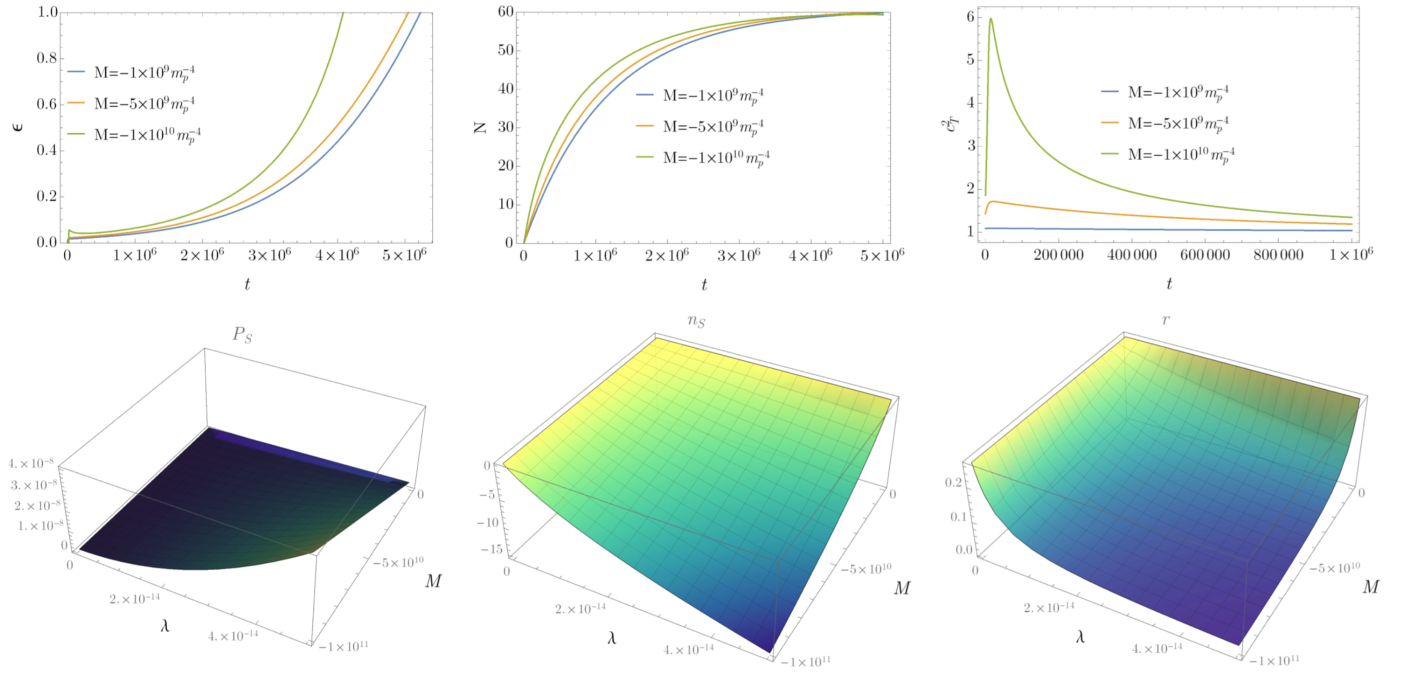
From which one can see the -dependence of the perturbation variables. Since is a negative value, one can see that when gets enlarged, it will cause an enhancement of (scalar spectrum) and a suppression of (tensor/scalar ratio) or vice versa, while (tensor spectrum) remains almost unchanged with regard to . For enough large so as that , one has
| (50) | |||||
| (51) | |||||
| (52) |
where one can see more clearly the relationship of , , . Moreover, for large , is expected to get smaller value in order to meet with the observational data.
In Fig. 1, we plot the evolutions of various background variables such as slow-roll parameter , the e-folding number and the sound speed squared of tensor perturbation of this model, with initial conditions chosen according to (46), considering three cases of being , , and . From the plot we can see that, although different in , all the three cases can have inflation for up to , while as grows, will deviate from unity. We also plot the perturbation variables such as the scalar power spectrum , its spectral index and the tensor/scalar ratio in terms of and , and we can see their dependence on and are consistent with the above analytical analysis.
In Fig. 2 we compare and in this model with the newest Planck observational data. We show that as grows, both and decrease (as also shown in the last plot), but has a faster speed. Although the decrease of tends to alleviate the dilemma of having too large for chaotic inflation models, it may not help much if one also wants to keep inside the allowable region. Maybe a better way is to have a more complicated form of disformal coupling with more parameters involved, however, this goes beyond the scope of the current study and can be postponed in the future.
III.2.2 Higgs inflation
We then consider the Higgs inflation, where it is proposed that inflaton is acted by the Higgs boson. Although the potential form is the same as that of chaotic inflation, due to the constraints from particle physics we have , which cannot guarantee the model be consistent with the constraints from cosmological observations. As has been suggested in [6], this problem can be circumvented by introducing a nonminal coupling term, namely in this model we have
| (53) |
Due to the involvement of , the analytical solution of and becomes complicated. However, since the usual case we can apply the approximation of , from which we get
| (54) |
while the scalar spectrum, spectral index and the tensor/scalar ratio are:
| (55) | |||||
| (56) | |||||
| (57) |
where the -dependence of the perturbation variables are the same as the first case, namely will not be changed by the involvement of nonminimal coupling. This can also be seen from the approximations for , where
| (58) | |||||
| (59) | |||||
| (60) |
On the other hand, it is known that in Higgs inflation, although is nearly fixed by the particle physics, the value of could be large enough to change the results. One can also obtain the approximations for large , namely , from (55)-(57), which are:
| (61) | |||||
| (62) | |||||
| (63) |
where all the dependence disappears. The reason might be that for large , the potential is so flattened to be closed to a constant, and any effects on the perturbations are dissipated away.
In Fig. 3, we plot the evolutions of slow-roll parameter , the e-folding number and the sound speed squared of tensor perturbation of this model, with initial conditions chosen according to (54), considering three cases of being , , and . From the plot we can see that, all three cases can also have inflation for up to , actually very close to each other, also deviates from unity as grows. The perturbation variables such as the scalar power spectrum , its spectral index and the tensor/scalar ratio are plotted as well, in terms of and , with their dependence on and consistent with the above analytical analysis.
In Fig. 4 we also compare and in this model with the observational data. Similar to the previous one, as grows, both and decrease, with faster. This means, while in this case the Higgs model allows and fall in the favorable region given by the observations, the involvement of tend to bring a smaller value of the spectral index.

III.2.3 monodromy inflation
The next example is the so-called monodromy inflation, in which we consider a power-law inflation potential with its index being a fraction, such as:
| (64) |
Such a potential arises when we take into account of the UV effects in inflation cosmology, such as those from string theory, where the back-reaction of other moduli field are also incorporated although the inflationary potential plays a leading role [61]. This is reasonable as the field excursion goes beyond the Planckian energy scale [62, 63]. Phenomenologically, such an inflation model is consistent with the Planck observational data, but with its location at the edge of the favorable region, indicating a little bit high spectral index. From the potential given above, we can get the initial values of and :
| (65) |
while the tensor spectrum, scalar spectrum and the tensor/scalar ratio are:
| (66) | |||||
| (67) | |||||
| (68) |
and when , we have:
| (69) | |||||
| (70) | |||||
| (71) |
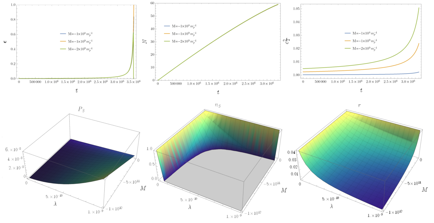
In Fig. 5, we plot the evolutions of slow-roll parameter , the e-folding number and the sound speed squared of tensor perturbation of this model, with initial conditions chosen according to (65), considering three cases of being , , and . The three cases can have inflation for up to as well, and also deviates from unity as grows. The perturbation variables such as the scalar power spectrum , its spectral index and the tensor/scalar ratio are plotted as well, in terms of and , with their dependence on and consistent with the above analytical analysis.
In Fig. 6 we also compare and in this model with the observational data. Although the model is favorable by Planck data, note that in [60] it has been shown that such a model is close to the edge of the favorable region. However, in our case, since both and decrease (with faster) as grows, it can make this model more close to the center of the favorable region. Namely, the model (and other models with larger than needed) can get improved by means of disformal coupling.
IV conclusion
In this paper, we investigate the inflation models with the so-called “disformal coupling” to gravity, which is based on the disformal transformation of two metrics. As an extension to conformal coupling, the disformal coupling also introduces the interaction of derivative terms of the field to the gravity part, which may bring interesting consequences. Therefore it is interesting to pursue for a better understanding of such a coupling.
We formulate the disformal coupling inflation model in its Jordan frame, including its Jordan frame action, the background equation of motion, as well as the perturbations, including tensor and scalar power spectrum , scalar spectral index as well as tensor/scalar ratio . We consider a simple example of coupling with only one additional parameter , and separate our analysis into two sides.
For models where the two “slow-roll conditions” are rigorously satisfied, we found that the apparent dependence of the disformal coupling in the expressions of , , and will be compensated by that in the expressions of initial conditions, and the final results will coincide with their Einstein frame counterpart, namely independent on the coupling. This result is in consistency with those in [24, 25, 26, 27], who claimed that the perturbations in two frames are invariant via disformal transformations. Moreover, letting to be real number put a further constraint on of . However, if the second “slow-roll condition” is not applied, e.g. when we choose “fixed values” of initial conditions independent of the disformal coupling, then the dependence of , and on the coupling will appear. We exemplified this with three common models, namely chaotic inflation, Higgs inflation, and monodromy inflation, and found that for all the three models, the enlargement of will amplify and reduce and , and vice versa. As is shown in our numerical results, this effect cannot help alleviate the dilemma of chaotic inflation, however it does have effect on making the monodromy inflation more favorable to the data. Since these models all belong to large field inflation model, albeit lack of rigid proof, it is reasonable to suspect if it is a general relationship for all the large inflation inflation models. Moreover, the sound speed of tensor and scalar perturbations are affected by the disformal coupling as well.
Although in [24, 25, 26, 27] it is shown that the perturbations are invariant under disformal transformations, it is still interesting to investigate in Jordan frame, which can show us the details of the dependence of parts of those variables on the coupling, and how it is compensated in a total. We expect it help us better understand the properties of those transformations and its applications to gravity theory and cosmology. Moreover, the superluminal behavior of the propagation speeds of scalar/tensor perturbations may also become a smoking gun. Although in general the existence of the superluminal behavior does not necessarily imply a violation of causality and formation of closed time-like curves (CTC) (see avoidance of CTC in [64, 65, 66, 67, 68]), it deserves further investigation in a general way. We will postpone these studies in future works.
Acknowledgements.
We thank Taishi Katsuragawa, Jun Chen, Ze Luan, Hua Chen and Zheng Fang for helpful discussions. This work was supported by the National Natural Science Foundation of China under Grants No. 11653002 and No. 11875141.Appendix A Action in the Jordan Frame
In the appendix, we will give some detailed formulation through which the Jordan frame action (5) is obtained. From the metric transformation of (1) and (3), one can first express the Christoffel symbol in Jordan frame as:
| (72) |
where
| (73) | |||||
| (74) | |||||
| (75) | |||||
According to the definition of Ricci scalar: , and after tedious calculation, we obtain the Ricci scalar:
| (76) | |||||
Therefore, action (2) can be transformed to the form:
| (77) | |||||
where we defined
| (78) | |||||
| (79) | |||||
Note that when , such action can be reduced to that presented in [34].
References
- [1] A. H. Guth, Phys. Rev. D 23, 347 (1981).
- [2] A. Albrecht and P. J. Steinhardt, Phys. Rev. Lett. 48, 1220 (1982); A. D. Linde, Phys. Lett. B 108, 389 (1982).
- [3] A. D. Linde, Phys. Lett. B 129 (1983) 177.
- [4] C. Brans and R. Dicke, Phys. Rev. 124 (1961), 925-935.
- [5] Y. Fujii and K. Maeda, Cambridge Monographs on Mathematical Physics, (Cambridge University Press, Cambridge; New York, 2003).
- [6] F. L. Bezrukov and M. Shaposhnikov, Phys. Lett. B 659, 703 (2008), arXiv:0710.3755 [hep-th].
- [7] L. Amendola,Phys. Lett. B 301, 175 (1993), arXiv:9302010 [gr-qc]; S. Capozziello and G. Lambiase, Gen. Rel. Grav. 31, 1005 (1999), arXiv:9901051 [gr-qc]; S. V. Sushkov, Phys. Rev. D 80, 103505 (2009), arXiv:0910.0980 [gr-qc]; L. N. Granda, JCAP 1007, 006 (2010), arXiv:0911.3702 [hep-th]; M. Minamitsuji, Phys. Rev. D 89, 064017 (2014), arXiv:1312.3759 [gr-qc]; Y. S. Myung, T. Moon and B. H. Lee, JCAP 1510, no. 10, 007 (2015), arXiv:1505.04027 [gr-qc]; T. Qiu, Phys. Rev. D 93 (2016) no.12, 123515, arXiv:1512.02887 [hep-th]; Y. Cai and Y. S. Piao, JHEP 1603, 134 (2016), arXiv:1601.07031 [hep-th].
- [8] N. Yang, Q. Fei, Q. Gao and Y. Gong, Class. Quant. Grav. 33 (2016) no.20, 205001, arXiv:1504.05839 [gr-qc].
- [9] C. Germani and A. Kehagias, Phys. Rev. Lett. 105,011302 (2010), arXiv:1003.2635 [hep-ph]; C. Germani and A. Kehagias, JCAP 1005, 019 (2010), Erratum-ibid. 1006, E01 (2010), arXiv:1003.4285 [astro-ph.CO].
- [10] K. Feng, T. Qiu and Y. Piao, Phys. Lett. B 729 (2014), 99-107, arXiv:1307.7864 [hep-th]; K. Feng and T. Qiu, Phys. Rev. D 90 (2014) no.12, 123508, arXiv:1409.2949 [hep-th]; T. Qiu and K. Feng, Eur. Phys. J. C 77 (2017) no.10, 687, arXiv:1608.01752 [hep-ph].
- [11] J. E. Lidsey and N. J. Nunes, Phys. Rev. D 67 (2003), 103510, arXiv:0303168 [astro-ph]; B. M. Carter and I. P. Neupane, JCAP 06 (2006), 004, arXiv:0512262 [hep-th].
- [12] J. Magueijo, T. Zlosnik and T. B. Kibble, Phys. Rev. D 87 (2013) no.6, 063504, arXiv:1212.0585 [astro-ph.CO]; S. Farnsworth, J. Lehners and T. Qiu, Phys. Rev. D 96 (2017) no.8, 083530, arXiv:1709.03171 [gr-qc].
- [13] Y. Cai, S. Chen, J. B. Dent, S. Dutta and E. N. Saridakis, Class. Quant. Grav. 28 (2011), 215011, arXiv:1104.4349 [astro-ph.CO]; T. Qiu, K. Tian and S. Bu, Eur. Phys. J. C 79 (2019) no.3, 261, arXiv:1810.04436 [gr-qc].
- [14] J. D. Bekenstein, Phys. Rev. D 48 (1993), 3641-3647, arXiv:9211017 [gr-qc].
- [15] M. Clayton and J. Moffat, Phys. Lett. B 460 (1999), 263-270, arXiv:9812481 [astro-ph]; M. Clayton and J. Moffat, Phys. Lett. B 477 (2000), 269-275, arXiv:gr-qc/9910112 [gr-qc].
- [16] B. A. Bassett, S. Liberati, C. Molina-Paris and M. Visser, Phys. Rev. D 62 (2000), 103518, arXiv:astro-ph/0001441 [astro-ph].
- [17] J. Magueijo, Rept. Prog. Phys. 66 (2003), 2025, arXiv:astro-ph/0305457 [astro-ph].
- [18] C. van de Bruck and G. Sculthorpe, Phys. Rev. D 87 (2013) no.4, 044004, arXiv:1210.2168 [astro-ph.CO].
- [19] P. Creminelli, J. Gleyzes, J. Noreña and F. Vernizzi, Phys. Rev. Lett. 113 (2014) no.23, 231301, arXiv:1407.8439 [astro-ph.CO].
- [20] N. Kaloper, Phys. Lett. B 583 (2004), 1-13, arXiv:hep-ph/0312002 [hep-ph].
- [21] C. van de Bruck, T. Koivisto and C. Longden, JCAP 03 (2016), 006, arXiv:1510.01650 [astro-ph.CO].
- [22] S. Sato and K. Maeda, Phys. Rev. D 97 (2018) no.8, 083512, arXiv:1712.04237 [gr-qc].
- [23] K. Karwan and P. Channuie, Phys. Rev. D 96 (2017) no.2, 023524, arXiv:1701.01267 [hep-ph].
- [24] M. Minamitsuji, Phys. Lett. B 737 (2014), 139-150, arXiv:1409.1566 [astro-ph.CO].
- [25] S. Tsujikawa, JCAP 04 (2015), 043, arXiv:1412.6210 [hep-th].
- [26] H. Motohashi and J. White, JCAP 02 (2016), 065, arXiv:1504.00846 [gr-qc].
- [27] G. Domènech, A. Naruko and M. Sasaki, JCAP 10 (2015), 067, arXiv:1505.00174 [gr-qc]
- [28] T. S. Koivisto, arXiv:0811.1957 [astro-ph].
- [29] M. Zumalacarregui, T. Koivisto, D. Mota and P. Ruiz-Lapuente, JCAP 05 (2010),. 038, arXiv:1004.2684 [astro-ph.CO].
- [30] T. S. Koivisto, D. F. Mota and M. Zumalacarregui, Phys. Rev. Lett. 109 (2012), 241102, arXiv:1205.3167 [astro-ph.CO].
- [31] T. Koivisto, D. Wills and I. Zavala, JCAP 06 (2014), 036, arXiv:1312.2597 [hep-th].
- [32] C. van de Bruck and J. Morrice, JCAP 04 (2015), 036, arXiv:1501.03073 [gr-qc].
- [33] D. Bettoni and S. Liberati, JCAP 08 (2015), 023, arXiv:1502.06613 [gr-qc].
- [34] J. Sakstein and S. Verner, Phys. Rev. D 92 (2015) no.12, 123005, arXiv:1509.05679 [gr-qc].
- [35] J. Mifsud and C. Van De Bruck, JCAP 11 (2017), 001, arXiv:1707.07667 [astro-ph.CO].
- [36] D. Bettoni, S. Liberati and L. Sindoni, JCAP 11 (2011), 007, arXiv:1108.1728 [gr-qc].
- [37] D. Bettoni, V. Pettorino, S. Liberati and C. Baccigalupi, JCAP 07 (2012), 027, arXiv:1203.5735 [astro-ph.CO].
- [38] N. Deruelle and J. Rua, JCAP 09 (2014), 002, arXiv:1407.0825 [gr-qc].
- [39] R. Hagala, C. Llinares and D. Mota, Astron. Astrophys. 585 (2016), A37, arXiv:1504.07142 [astro-ph.CO].
- [40] J. Gleyzes, D. Langlois, M. Mancarella and F. Vernizzi, JCAP 08 (2015), 054, arXiv:1504.05481 [astro-ph.CO].
- [41] C. de Rham and G. Gabadadze, Phys. Rev. D 82 (2010), 044020, arXiv:1007.0443 [hep-th]]; C. de Rham, G. Gabadadze and A. J. Tolley, Phys. Rev. Lett. 106 (2011), 231101, arXiv:1011.1232 [hep-th].
- [42] R. Gannouji, M. W. Hossain, N. Jaman and M. Sami, Phys. Rev. D 99 (2019) no.4, 043504, arXiv:1808.04137 [gr-qc].
- [43] D. Bettoni and S. Liberati, Phys. Rev. D 88 (2013), 084020, arXiv:1306.6724 [gr-qc].
- [44] M. Zumalacárregui and J. García-Bellido, ” Phys. Rev. D 89 (2014), 064046, arXiv:1308.4685 [gr-qc].
- [45] J. Gleyzes, D. Langlois, F. Piazza and F. Vernizzi, JCAP 02 (2015), 018, arXiv:1408.1952 [astro-ph.CO].
- [46] A. De Felice and S. Tsujikawa, Phys. Rev. D 91 (2015) no.10, 103506, arXiv:1411.0736 [hep-th].
- [47] D. Bettoni and M. Zumalacárregui, Phys. Rev. D 91 (2015), 104009, arXiv:1502.02666 [gr-qc].
- [48] C. van de Bruck, J. Morrice and S. Vu, Phys. Rev. Lett. 111 (2013), 161302, arXiv:1303.1773 [astro-ph.CO].
- [49] P. Brax, C. Burrage, A. Davis and G. Gubitosi, JCAP 11 (2013), 001, arXiv:1306.4168 [astro-ph.CO].
- [50] P. Brax and C. Burrage, Phys. Rev. D 90 (2014) no.10, 104009, arXiv:1407.1861 [astro-ph.CO].
- [51] J. Sakstein, JCAP 12 (2014), 012, arXiv:1409.1734 [astro-ph.CO].
- [52] P. Brax, C. Burrage and C. Englert, Phys. Rev. D 92 (2015) no.4, 044036, arXiv:1506.04057 [hep-ph].
- [53] P. Brax and A. Davis, Phys. Rev. D 98 (2018) no.6, 063531, arXiv:1809.09844 [gr-qc].
- [54] C. Dalang and L. Lombriser, JCAP 10 (2019) no.10, 013, arXiv:1906.12333 [astro-ph.CO].
- [55] J. Sakstein, Doctoral thesis, arXiv:1502.04503 [astro-ph.CO]; S. Vu, arXiv:1502.00930 [astro-ph.CO].
- [56] M. Zumalacarregui, T. S. Koivisto and D. F. Mota, Phys. Rev. D 87 (2013), 083010, arXiv:1210.8016 [astro-ph.CO].
- [57] T. Kobayashi, M. Yamaguchi and J. Yokoyama, Prog. Theor. Phys. 126 (2011), 511-529, arXiv:1105.5723 [hep-th].
- [58] A. De Felice and S. Tsujikawa, Phys. Rev. D 84 (2011), 083504, arXiv:1107.3917 [gr-qc].
- [59] W. H. Kinney, Phys. Rev. D 72, 023515 (2005), arXiv:0503017 [gr-qc]; H. Motohashi, A. A. Starobinsky and J. Yokoyama, JCAP 1509, 018 (2015), arXiv:1411.5021 [astro-ph.CO]; Z. Yi and Y. Gong, JCAP 1803, 052 (2018), arXiv:1712.07478 [gr-qc]; M. H. Namjoo, H. Firouzjahi and M. Sasaki, EPL 101, no. 3, 39001 (2013), arXiv:1210.3692 [astro-ph.CO]; J. Martin, H. Motohashi and T. Suyama, Phys. Rev. D 87, no. 2, 023514 (2013), arXiv:1211.0083 [astro-ph.CO].
- [60] Y. Akrami et al. [Planck], arXiv:1807.06211 [astro-ph.CO].
- [61] L. McAllister, E. Silverstein, A. Westphal and T. Wrase, JHEP 09 (2014), 123, arXiv:1405.3652 [hep-th].
- [62] E. Silverstein and A. Westphal, Phys. Rev. D 78 (2008), 106003, arXiv:0803.3085 [hep-th].
- [63] L. McAllister, E. Silverstein and A. Westphal, Phys. Rev. D 82 (2010), 046003, arXiv:0808.0706 [hep-th].
- [64] S. Hawking, Phys. Rev. D 46 (1992), 603-611..
- [65] E. Babichev, V. Mukhanov and A. Vikman, JHEP 02 (2008), 101, arXiv:0708.0561 [hep-th].
- [66] J. Bruneton, Phys. Rev. D 75 (2007), 085013, arXiv:gr-qc/0607055 [gr-qc]; R. Geroch, arXiv:1005.1614 [gr-qc].
- [67] J. Evslin and T. Qiu, JHEP 11 (2011), 032, arXiv:1106.0570 [hep-th]; J. Evslin, JHEP 03 (2012), 009, arXiv:1112.1349 [hep-th].
- [68] C. Burrage, C. de Rham, L. Heisenberg and A. J. Tolley, JCAP 07 (2012), 004, arXiv:1111.5549 [hep-th].