A Span-based Linearization for Constituent Trees
Abstract
We propose a novel linearization of a constituent tree, together with a new locally normalized model. For each split point in a sentence, our model computes the normalizer on all spans ending with that split point, and then predicts a tree span from them. Compared with global models, our model is fast and parallelizable. Different from previous local models, our linearization method is tied on the spans directly and considers more local features when performing span prediction, which is more interpretable and effective. Experiments on PTB (95.8 F1) and CTB (92.4 F1) show that our model significantly outperforms existing local models and efficiently achieves competitive results with global models.
1 Introduction
Constituent parsers map natural language sentences to hierarchically organized spans (Cross and Huang 2016). According to the complexity of decoders, two types of parsers have been studied, globally normalized models which normalize probability of a constituent tree on the whole candidate tree space (e.g. chart parser (Stern et al. 2017a)) and locally normalized models which normalize tree probability on smaller subtrees or spans. It is believed that global models have better parsing performance (Gaddy et al. 2018). But with the fast development of neural-network-based feature representations (Hochreiter and Schmidhuber 1997; Vaswani et al. 2017), local models are able to get competitive parsing accuracy while enjoying fast training and testing speed, and thus become an active research topic in constituent parsing.
Locally normalized parsers usually rely on tree decompositions or linearizations. From the perspective of decomposition, the probability of trees can be factorized, for example, on individual spans. Teng and Zhang 2018 investigates such a model which predicts probability on each candidate span. It achieves quite promising parsing results, while the simple local probability factorization still leaves room for improvements. From the perspective of linearization, there are many ways to transform a structured tree into a shallow sequence. As a recent example, Shen et al. 2018 linearizes a tree with a sequence of numbers, each of which indicates words’ syntactic distance in the tree (i.e., height of the lowest common ancestor of two adjacent words). Similar ideas are also applied in Vinyals et al. 2015, Choe and Charniak 2016 and transition-based systems (Cross and Huang 2016; Liu and Zhang 2017a). With tree linearizations, the training time can be further accelerated to , but the parsers often sacrifice a clear connection with original spans in trees, which makes both features and supervision signals from spans hard to use.
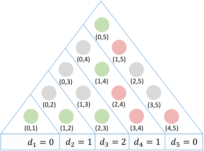
In this work, we propose a novel linearization of constituent trees tied on their span representations. Given a sentence and its parsing tree , for each split point after in the sentence, we assign it a parsing target , where is the longest span ending with in . We can show that, for a binary parsing tree, the set includes all left child spans in . Thus the linearization is actually sufficient to recover a parsing tree of the sentence.
Compared with prior work, the linearization is directly based on tree spans, which might make estimating model parameters easier. We also build a different local normalization compared with the simple per-span-normalization in Teng and Zhang 2018. Specifically, the probability is normalized on all candidate split points on the left of . The more powerful local model can help to further improve parsing performance while retaining the fast learning and inference speed (with a greedy heuristic for handling illegal sequences, we can achieve average inference complexity). We perform experiments on PTB and CTB. The proposed parser significantly outperforms existing locally normalized models, and achieves competitive results with state-of-the-art global models (95.8 F1 on PTB and 92.4 F1 on CTB). We also evaluate how the new linearization helps parse spans with different lengths and types.
To summarize, our main contributions include:
- •
Proposing a new linearization which has clear interpretation (Section 2).
- •
Building a new locally normalized model with constraints on span scores (Section 3).
- •
Compared with previous local models, the proposed parser achieves better performance (competitive with global models) and has faster parsing speed (Section 4).
2 Tree Linearization
We first prepare some notations. Let be a sentence, be its binary constituent tree and be a derivation in . Denote to be a span from to (for simplicity, we ignore the label of a span).
Definition 1.
Given a sentence and its tree , we call a linearization of , where and is the longest span ending with in .
Clearly, there is only one such linearization for a tree. We have an equal definition of , which shows the span is a left child span.
Proposition 1.
Given a tree , the set of spans is equal to the set of left child spans 11 1 The root node is also regarded as a left child span.
Proof.
First, for each , there is only one left child span ending with , otherwise if is a left child span with (e.g. ), must also be a right child span. Therefore . Similarly, if , should be a right child span of . ∎
Thus we can generate the linearization using Algorithm 1. For span and its gold split , we can get . Then we recursively calculate the linearization of span and . Note that the returned linearization does not contain , so we append zero ( for the root node) to the end as the final linearization. Figure 1 is a generation process of sentence “She loves writing code .”. From the span table, it is obvious that there is only one left child span (green circles) ending with the same right boundary.
In the following discussions, we will use and interchangeably. Next, we show two properties of a legal .
Proposition 2.
A linearization can recover a tree iff.
- 1.
.
- 2.
is not in the range , .
Proof.
The necessity is obvious. We show the sufficiency by induction on the sentence length. When , the conclusion stands. Assuming for all linearizations with length less than , property 1 and 2 lead to a well-formed tree, and now consider a linearization with length .
Define . Since (by property 1), is not none. We split the sentence into , , and claim that after removing , the spans in are either in or , thus by induction we obtain the conclusion. To validate the claim, for , by property 1, we have , thus is in . For , by property 2, either or . Since is the largest index with , we have , which means is in . Therefore, we show the existence of a tree from . The tree is also unique, because if two trees and have the same linearization, by Proposition 1, we have . ∎
Proposition 2 also suggests a top-down algorithm (Algorithm 2) for performing tree inference given a legal linearization. For span (with label ), we find the rightmost split satisfying , and then recursively decode the two sub-trees rooted at span and , respectively. When does not satisfy property 2 (our model can ensure property 1), one solution is to seek a minimum change of to make it legal. However, it is reduced to a minimum vertex cover problem (regarding each span as a point, if two spans violate property 2, we connect an edge between them. ). We can also slightly modify Algorithm 2 to perform an approximate inference (Section 3.4).
Finally we need to deal with the linearization of non-binary trees. For spans having more than two child spans, there is no definition for their middle child spans whether they are left children or right children, thus Proposition 1 might not stand. We recursively combine two adjacent spans from right to left using an empty label . Then the tree can be converted to a binary tree (Stern et al. 2017a). For a unary branch, we treat it as a unique span with a new label which concatenates all the labels in the branch.
3 The Parser
In this section, we introduce our encoder, decoder and inference algorithms in detail. Then we compare our normalization method with two other methods, globally normalized and existing locally normalized methods.
3.1 Encoder
We represent each word using three pieces of information, a randomly initialized word embedding , a character-based embedding obtained by a character-level LSTM and a randomly initialized part-of-speech tag embedding . We concatenate these three embeddings to generate a representation of word ,
To get the representation of the split points, the word representation matrix is fed into a bidirectional LSTM or Transformer (Vaswani et al. 2017) firstly. Then we calculate the representation of the split point between and using the outputs from the encoders,
| (1) |
Note that for Transformer encoder, is calculated in the same way as Kitaev and Klein 2018a.
3.2 Decoder
Since a split point can play two different roles when it is the left or right boundary of a span, we use two different vectors to represent the two roles inspired by Dozat and Manning 2017. Concretely, we use two multi-layer perceptrons to generate two different representations,
| (2) |
Then we can define the score of span using a biaffine attention function (Dozat and Manning 2017; Li et al. 2019),
where , and are all model parameters. measures the possibility of being a left child span in the tree.
Different from Stern et al. 2017a which does global normalization on the probability of the whole tree and Teng and Zhang 2018 which does local normalization on each candidate span, we do normalization on all spans with the same right boundary . Thus the probability of span to be a left child span is defined as,
| (3) |
Finally, we can predict the linearization using the probability ,
| (4) |
For label prediction, we first infer the tree structure from the linearization (Section 3.4). 22 2 Note that we would perform label prediction without the tree inference step which will train the entire parser in linear time as sequence labelling models (Gómez-Rodríguez and Vilares 2018), but we empirically find that the tree structure helps improving the label classifier. Then we use a multi-layer perceptron to calculate the label probability of span ,
Final predicted label of span is .
3.3 Training Objective
Given a gold parsing tree and its linearization , we can calculate the loss using the negative log-likelihood:
The loss function consists of two parts. One is the structure loss, which is only defined on the left child spans. The other one is the label loss, which is defined on all the spans in .
3.4 Tree Inference
To reconstruct the tree structure from the predicted linearization , we must deal with illegal sequences. One solution is to convert an illegal linearization to a legal one, and then use Algorithm 2 to recover the tree. However, the optimal converting algorithm is NP hard as discussed in Section 2. We propose two approximate reconstruction methods, both of which are based on replacing line 5 of Algorithm 2. One is to find the largest satisfying ,
The other is to find the index of the smallest (if there are multiple choices, we choose the largest one),
Both methods are applicable to legal situations, and they have similar performance in our empirical evaluations. The inference time complexity is in the worst-case for unbalanced trees, while in average it is (which is the same as Stern et al. 2017a).
Finally, instead of reconstructing trees from linearization sequences , we could have an accurate CKY-style decoding algorithm from probabilities (Equation 3). Specifically, it maximizes the product of left child span probabilities,
where represents the highest probability of subtree with root node . We can calculate using dynamic programming algorithm and back-trace the tree accordingly. The complexity is .
3.5 More Discussions on Normalization
We can compare our locally normalized model (Equation 3) with other probability factorizations of constituent trees (Figure 2).
Global normalization (Figure 2(a)) performs marginalization over all candidate trees, which requires dynamic programming decoding. As a local model, our parser is a span-level factorization of the tree probability, and each factor only marginalizes over a linear number of items (i.e., the probability of span is normalized with all scores of ). It is easier to be parallelized and enjoys a much faster parsing speed. We will show that its performance is also competitive with global models.
Teng and Zhang 2018 studies two local normalized models over spans, namely the span model and the rule model. The span model simply considers individual spans independently (Figure 2(b)) which may be the finest factorization. Our model lies between it and the global model.
The rule model considers a similar normalization with our model. If it is combined with the top-down decoding (Stern et al. 2017a), the two parsers look similar. 33 3 We thank an anonymous reviewer for pointing out the connection. The following discussions are based on his/her detailed reviews. We discuss their differences. The rule model takes all ground truth spans from the gold trees, and for each span , it compiles a probability for its ground truth split . Our parser, on the other side, factorizes on each word. Therefore, for the same span , their normalization is constrained within , while ours is over all . The main advantage of our parser is simpler span representations (not depend on parent spans): it makes the parser easy to batch for sentences with different lengths and tree structures since each can be calculated offline before training.
4 Experiments
| Type | NP | VP | S | PP | SBAR | ADVP | ADJP | QP | WHNP |
|---|---|---|---|---|---|---|---|---|---|
| Count | 18630 | 8743 | 5663 | 5492 | 1797 | 1213 | 893 | 490 | 429 |
| PSN Model | 93.15 | 91.81 | 91.21 | 89.73 | 87.81 | 86.89 | 73.01 | 89.80 | 97.20 |
| Our Model | 93.42 | 92.62 | 91.95 | 89.91 | 88.93 | 87.39 | 75.14 | 91.63 | 97.44 |
| Difference | +0.27 | +0.81 | +0.74 | +0.18 | +1.12 | +0.50 | +2.13 | +1.83 | +0.24 |
4.1 Data and Settings
Datasets and Preprocessing
All models are trained on two standard benchmark treebanks, English Penn Treebank (PTB) (Marcus et al. 1993) and Chinese Penn Treebank (CTB) 5.1. The POS tags are predicted using Stanford Tagger (Toutanova et al. 2003). To clean the treebanks, we strip the leaf nodes with POS tag -NONE- from the two treebanks and delete the root nodes with constituent type ROOT. For evaluating the results, we use the standard evaluation tool 44 4 http://nlp.cs.nyu.edu/evalb/.
For words in the testing corpus but not in the training corpus, we replace them with a unique label <UNK>. We also replace the words in the training corpus with the unknown label <UNK> with probability , where is the number of time word appears in the training corpus and we set as Cross and Huang 2016.
Hyperparameters
We use 100D GloVe embedding for PTB (Pennington et al. 2014). For character encoding, we randomly initialize the character embeddings with dimension 64.
We use Adam optimizer with initial learning rate 1.0 and epsilon . For LSTM encoder, we use a hidden size of 1024, with 0.2 dropout in all the feed-forward and recurrent connections. For Transformer encoder, we use the same hyperparameters as Kitaev and Klein 2018a. For split point representation, we apply two 1024-dimensional hidden size feed-forward networks. All the dropout we use in the decoder layer is 0.33. We also use BERT (Devlin et al. 2019) (uncased, 24 layers, 16 attention heads per layer and 1024-dimensional hidden vectors) and use the output of the last layer as the pre-trained word embeddings. 55 5 The source code for our model is publicly available: https://github.com/AntNLP/span-linearization-parser
Training Details
We use PyTorch as our neural network toolkit and run the code on a NVIDIA GeForce GTX Titan Xp GPU and Intel Xeon E5-2603 v4 CPU. All models are trained for up to 150 epochs with batch size 150 (Zhou and Zhao 2019).
| Model | LR | LP | F1 |
|---|---|---|---|
| Global Model | |||
| Stern et al. 2017a | 90.6 | 93.0 | 91.8 |
| Gaddy et al. 2018 | - | - | 92.1 |
| Kitaev and Klein 2018a♠ | 93.2 | 93.9 | 93.6 |
| Zhou and Zhao 2019♠ | 93.6 | 93.9 | 93.8 |
| Local Model | |||
| Vilares et al. 2019 | - | - | 90.6 |
| Liu et al. 2018 | - | - | 91.2 |
| Ma et al. 2017 | - | - | 91.5 |
| Shen et al. 2018 | 91.7 | 92.0 | 91.8 |
| Liu and Zhang 2017a | - | - | 91.8 |
| Hong and Huang 2018 | 91.5 | 92.5 | 92.0 |
| Teng and Zhang 2018 | 92.2 | 92.5 | 92.4 |
| Dyer et al. 2016♡ | - | - | 92.4 |
| Stern et al. 2017b♡ | 92.6 | 92.6 | 92.6 |
| Our Model | 92.3 | 92.9 | 92.6 |
| Our Model♠ | 93.3 | 94.1 | 93.7 |
| Pre-training/Ensemble/Re-ranking | |||
| Liu et al. 2018 | - | - | 92.3 |
| Choe and Charniak 2016 | - | - | 93.8 |
| Liu and Zhang 2017a | - | - | 94.2 |
| Fried et al. 2017 | - | - | 94.7 |
| Kitaev and Klein 2018a♠ | 94.9 | 95.4 | 95.1 |
| Kitaev and Klein 2018b♠ | 95.5 | 95.7 | 95.6 |
| Zhou and Zhao 2019♠ | 95.7 | 96.0 | 95.8 |
| Our Model (+BERT) | 95.6 | 96.0 | 95.8 |
| Our Model (+BERT)♠ | 95.5 | 96.1 | 95.8 |
| Model | LR | LP | F1 |
|---|---|---|---|
| Global Model | |||
| Kitaev and Klein 2018b♠ | 91.6 | 92.0 | 91.8 |
| Zhou and Zhao 2019♠ | 92.0 | 92.3 | 92.2 |
| Local Model | |||
| Dyer et al. 2016 | - | - | 84.6 |
| Liu et al. 2018 | - | - | 85.4 |
| Liu and Zhang 2017b | 85.2 | 85.9 | 85.5 |
| Vilares et al. 2019 | - | - | 85.6 |
| Liu and Zhang 2017a | - | - | 86.1 |
| Shen et al. 2018 | 86.4 | 86.6 | 86.5 |
| Fried and Klein 2018 | - | - | 87.0 |
| Teng and Zhang 2018 | 87.1 | 87.5 | 87.3 |
| Our Model | 92.2 | 92.7 | 92.4 |
| Our Model♠ | 92.1 | 92.3 | 92.2 |
4.2 Main Results
Table 2 shows the final results on PTB test set. Our models (92.6 F1 with LSTM, 93.7 F1 with Transformer) significantly outperform the single locally normalized models. Compared with globally normalized models, our models also outperform those parsers with LSTM encoder and achieve a competitive result with Transformer encoder parsers. With the help of BERT (Devlin et al. 2018), our models with two encoders both achieve the same performance (95.8 F1) as the best parser (Zhou and Zhao 2019). Table 3 shows the final results on CTB test set. Our models (92.4 F1) also significantly outperform local models and achieve competitive result amongst global models.
Compared with Teng and Zhang 2018 which does local normalization on single span, our model increases 0.2 F1 on PTB, which shows that doing normalization on more spans is really better. Our model also significantly outperforms Shen et al. 2018 which predicts the syntactic distance of a tree. This indicates the superiority of our linearization method directly tied on the spans.
4.3 Evaluation
To better understand the extent to which our model transcends the locally normalized model which does normalization on a single span described in Teng and Zhang 2018, we do several experiments to compare the performance about different lengths of spans and different constituent types.
In order to make a fair comparison, we implement their model by ourselves using the same LSTM encoder as ours. Besides, we ignore the LSTM for label prediction and complex span representations in their models and use simpler settings. Our own implementation achieves the same result as they report (92.4 F1). For convenience, we call their model per-span-normalization (PSN for short) model in the following.
Influence of Span Length
First, we analyse the influence of different lengths of spans and the results are shown in Figure 3. We find that for sentences of lengths between , our model significantly outperforms PSN model. For short spans, PSN model only needs to consider few spans, which is more local and it is enough for the per-span-normalization to handle this situation. For long spans, our model needs to do normalization on more spans and the state space becomes large linearly. So the accuracy decreases fast, and there is no advantage compared with PSN model which uses CKY algorithm for inference. For spans of other lengths, our locally normalized method can take all spans with the same right boundary into consideration and add sum-to-one constraints on their scores. As a result, our model outperforms PSN model even without the help of accurate inference.
| Model | LR | LP | F1 |
|---|---|---|---|
| Full model | 92.31 | 92.87 | 92.59 |
| - and | 92.15 | 92.72 | 92.43 |
| - normalization | 91.25 | 92.93 | 92.08 |
| + label linearization | 90.79 | 91.56 | 91.17 |
Influence of Constituent Type
Then we compare the accuracy of different constituent types. Table 1 shows the results of nine types which occur most frequently. Our model all performs better than PSN model, especially in types SBAR, ADJP and QP. When optimizing the representation of one split point, our model can consider all of the words before it, which can be helpful to predict some types. For example, when we predict an adjective phrase (ADJP), its representation has fused the words’ information before it (e.g. linking verb like “is”), which can narrow the scope of prediction.
4.4 Ablation Study
| Inference Algorithm | LR | LP | F1 |
|---|---|---|---|
| 92.31 | 92.87 | 92.59 | |
| 92.39 | 92.75 | 92.57 | |
| 91.93 | 93.21 | 92.57 |
| Model | sents/sec |
|---|---|
| Global Model | |
| Stern et al. 2017a | 20 |
| Kitaev and Klein 2018a♠ (w. Cython) | 150 |
| Zhou and Zhao 2019♠ (w. Cython) | 159 |
| Local Model | |
| Teng and Zhang 2018 | 22 |
| Stern et al. 2017a | 76 |
| Liu and Zhang 2017b | 79 |
| Shen et al. 2018 | 111 |
| Shen et al. 2018 (w/o tree inference) | 351 |
| Vilares et al. 2019 | 942 |
| Our Model | 220 |
| Our Model♠ | 155 |
We perform several ablation experiments by modifying the structure of the decoder layer. The results are shown in Table 4.
First, we delete the two different split point representations described in Equation (2) and directly use the output of LSTM as the final representation. Final performance slightly decreases, which indicates that distinguishing the representations of left and right boundaries of a span is really helpful.
Then we delete the local normalization on partial spans and only calculate the probability of each span to be a left child. The inference algorithm is the same as our full model. Final result decreases by 0.5 F1, despite improvement on precision. This might be because our normalization method can add constraints on all the spans with the same right boundary, which makes it effective when only one span is correct.
Finally, we try to predict the labels sequentially, which means assigning each split a tuple , where and represent the labels of the longest spans ending and starting with in the tree, respectively. This may make our model become a sequence labeling model similar to Gómez-Rodríguez and Vilares 2018. However, the performance is very poor, and this is largely due to the loss of structural information in the label prediction. Therefore, how to balance efficiency and label prediction accuracy might be a research problem in the future.
4.5 Inference Algorithms
We compare three inference algorithms described in Section 3.4. The results are shown in Table 5. We find that different inference algorithms have no obvious effect on the performance, mainly due to the powerful learning ability of our model. Thus we use the third method which is the most convenient to implement.
4.6 Parsing Speed
The parsing speeds of our parser and other parsers are shown in Table 6. Although our inference complexity is , our speed is faster than other local models, except Shen et al. 2018 which evaluates without tree inference and Vilares et al. 2019 which utilizes a pure sequence tagging framework. This is mainly due to the simplicity of our model and the parallelism of matrix operations for structure prediction. Compared with globally normalized parsers like Zhou and Zhao 2019 and Kitaev and Klein 2018a, our model is also faster even if they use optimization for python code (e.g. Cython 66 6 https://cython.org/). Other global model like Stern et al. 2017a which infers in complexity is much slower than ours, and this shows the superiority of our linearization in speed.
5 Related Work
Globally normalized parsers often have high performance on constituent parsing due to their search on the global state space (Stern et al. 2017a; Kitaev and Klein 2018a; Zhou and Zhao 2019). However, they suffer from high time complexity and are difficult to parallelize. Thus many efforts have been made to optimize their efficiency (Vieira and Eisner 2017).
Recently, the rapid development of encoders (Hochreiter and Schmidhuber 1997; Vaswani et al. 2017) and pre-trained language models (Devlin et al. 2018) have enabled local models to achieve similar performance as global models. Teng and Zhang 2018 propose two local models, one does normalization on each candidate span and one on each grammar rule. Their models even outperform the global model in Stern et al. 2017a thanks to the better representation of spans. However, they still need an complexity inference algorithm to reconstruct the final parsing tree.
Meanwhile, many work do research on faster sequential models. Transition-based models predict a sequence of actions and achieve an complexity (Watanabe and Sumita 2015; Cross and Huang 2016; Liu and Zhang 2017a). However, they suffer from the issue of error propagation and cannot be parallel. Sequence labeling models regard tree prediction as sequence prediction problem (Gómez-Rodríguez and Vilares 2018; Shen et al. 2018). These models have high efficiency, but their linearizations have no direct relation to the spans, so the performance is much worse than span-based models.
We propose a novel linearization method closely related to the spans and decode the tree in complexity. Compared with Teng and Zhang 2018, we do normalization on more spans, thus achieve a better performance.
In future work, we will apply graph neural network (Velickovic et al. 2018; Ji et al. 2019; Sun et al. 2019) to enhance the span representation. Due to the excellent properties of our linearization, we can jointly learn constituent parsing and dependency parsing in one graph-based model. In addition, there is also a right linearization defined on the set of right child spans. We can study how to combine the two linear representations to further improve the performance of the model.
6 Conclusion
In this work, we propose a novel linearization of constituent trees tied on the spans tightly. In addition, we build a new normalization method, which can add constraints on all the spans with the same right boundary. Compared with previous local normalization methods, our method is more accurate for considering more span information, and reserves the fast running speed due to the parallelizable linearization model. The experiments show that our model significantly outperforms existing local models and achieves competitive results with global models.
Acknowledgments
The authors would like to thank the reviewers for their helpful comments and suggestions. The authors would also like to thank Tao Ji and Changzhi Sun for their advices on models and experiments. The corresponding author is Yuanbin Wu. This research is (partially) supported by STCSM (18ZR1411500), the Foundation of State Key Laboratory of Cognitive Intelligence, iFLYTEK(COGOS-20190003), and an open research fund of KLATASDS-MOE.
References
- Choe and Charniak (2016) Do Kook Choe and Eugene Charniak. 2016. Parsing as language modeling. In Proceedings of the 2016 Conference on Empirical Methods in Natural Language Processing, EMNLP 2016, Austin, Texas, USA, November 1-4, 2016, pages 2331–2336. The Association for Computational Linguistics.
- Cross and Huang (2016) James Cross and Liang Huang. 2016. Span-based constituency parsing with a structure-label system and provably optimal dynamic oracles. In Proceedings of the 2016 Conference on Empirical Methods in Natural Language Processing, EMNLP 2016, Austin, Texas, USA, November 1-4, 2016, pages 1–11.
- Devlin et al. (2018) Jacob Devlin, Ming-Wei Chang, Kenton Lee, and Kristina Toutanova. 2018. BERT: pre-training of deep bidirectional transformers for language understanding. CoRR, abs/1810.04805.
- Devlin et al. (2019) Jacob Devlin, Ming-Wei Chang, Kenton Lee, and Kristina Toutanova. 2019. BERT: pre-training of deep bidirectional transformers for language understanding. In Proceedings of the 2019 Conference of the North American Chapter of the Association for Computational Linguistics: Human Language Technologies, NAACL-HLT 2019, Minneapolis, MN, USA, June 2-7, 2019, Volume 1 (Long and Short Papers), pages 4171–4186. Association for Computational Linguistics.
- Dozat and Manning (2017) Timothy Dozat and Christopher D. Manning. 2017. Deep biaffine attention for neural dependency parsing. In 5th International Conference on Learning Representations, ICLR 2017, Toulon, France, April 24-26, 2017, Conference Track Proceedings. OpenReview.net.
- Dyer et al. (2016) Chris Dyer, Adhiguna Kuncoro, Miguel Ballesteros, and Noah A. Smith. 2016. Recurrent neural network grammars. In NAACL HLT 2016, The 2016 Conference of the North American Chapter of the Association for Computational Linguistics: Human Language Technologies, San Diego California, USA, June 12-17, 2016, pages 199–209.
- Fried and Klein (2018) Daniel Fried and Dan Klein. 2018. Policy gradient as a proxy for dynamic oracles in constituency parsing. In Proceedings of the 56th Annual Meeting of the Association for Computational Linguistics, ACL 2018, Melbourne, Australia, July 15-20, 2018, Volume 2: Short Papers, pages 469–476.
- Fried et al. (2017) Daniel Fried, Mitchell Stern, and Dan Klein. 2017. Improving neural parsing by disentangling model combination and reranking effects. In Proceedings of the 55th Annual Meeting of the Association for Computational Linguistics, ACL 2017, Vancouver, Canada, July 30 - August 4, Volume 2: Short Papers, pages 161–166. Association for Computational Linguistics.
- Gaddy et al. (2018) David Gaddy, Mitchell Stern, and Dan Klein. 2018. What’s going on in neural constituency parsers? an analysis. In Proceedings of the 2018 Conference of the North American Chapter of the Association for Computational Linguistics: Human Language Technologies, NAACL-HLT 2018, New Orleans, Louisiana, USA, June 1-6, 2018, Volume 1 (Long Papers), pages 999–1010.
- Gómez-Rodríguez and Vilares (2018) Carlos Gómez-Rodríguez and David Vilares. 2018. Constituent parsing as sequence labeling. In Proceedings of the 2018 Conference on Empirical Methods in Natural Language Processing, Brussels, Belgium, October 31 - November 4, 2018, pages 1314–1324.
- Hochreiter and Schmidhuber (1997) Sepp Hochreiter and Jürgen Schmidhuber. 1997. Long short-term memory. Neural Computation, 9(8):1735–1780.
- Hong and Huang (2018) Juneki Hong and Liang Huang. 2018. Linear-time constituency parsing with rnns and dynamic programming. In Proceedings of the 56th Annual Meeting of the Association for Computational Linguistics, ACL 2018, Melbourne, Australia, July 15-20, 2018, Volume 2: Short Papers, pages 477–483.
- Ji et al. (2019) Tao Ji, Yuanbin Wu, and Man Lan. 2019. Graph-based dependency parsing with graph neural networks. In Proceedings of the 57th Conference of the Association for Computational Linguistics, ACL 2019, Florence, Italy, July 28- August 2, 2019, Volume 1: Long Papers, pages 2475–2485. Association for Computational Linguistics.
- Kitaev and Klein (2018a) Nikita Kitaev and Dan Klein. 2018a. Constituency parsing with a self-attentive encoder. In Proceedings of the 56th Annual Meeting of the Association for Computational Linguistics, ACL 2018, Melbourne, Australia, July 15-20, 2018, Volume 1: Long Papers, pages 2675–2685.
- Kitaev and Klein (2018b) Nikita Kitaev and Dan Klein. 2018b. Multilingual constituency parsing with self-attention and pre-training. CoRR, abs/1812.11760.
- Li et al. (2019) Ying Li, Zhenghua Li, Min Zhang, Rui Wang, Sheng Li, and Luo Si. 2019. Self-attentive biaffine dependency parsing. In Proceedings of the Twenty-Eighth International Joint Conference on Artificial Intelligence, IJCAI 2019, Macao, China, August 10-16, 2019, pages 5067–5073. ijcai.org.
- Liu and Zhang (2017a) Jiangming Liu and Yue Zhang. 2017a. In-order transition-based constituent parsing. Transactions of the Association for Computational Linguistics, 5:413–424.
- Liu and Zhang (2017b) Jiangming Liu and Yue Zhang. 2017b. Shift-reduce constituent parsing with neural lookahead features. Transactions of the Association for Computational Linguistics, 5:45–58.
- Liu et al. (2018) Lemao Liu, Muhua Zhu, and Shuming Shi. 2018. Improving sequence-to-sequence constituency parsing. In Proceedings of the Thirty-Second AAAI Conference on Artificial Intelligence, (AAAI-18), the 30th innovative Applications of Artificial Intelligence (IAAI-18), and the 8th AAAI Symposium on Educational Advances in Artificial Intelligence (EAAI-18), New Orleans, Louisiana, USA, February 2-7, 2018, pages 4873–4880. AAAI Press.
- Ma et al. (2017) Chunpeng Ma, Akihiro Tamura, Lemao Liu, Tiejun Zhao, and Eiichiro Sumita. 2017. Improving feature-rich transition-based constituent parsing using recurrent neural networks. IEICE Transactions, 100-D(9):2205–2214.
- Marcus et al. (1993) Mitchell P. Marcus, Beatrice Santorini, and Mary Ann Marcinkiewicz. 1993. Building a large annotated corpus of english: The penn treebank. Computational Linguistics, 19(2):313–330.
- Pennington et al. (2014) Jeffrey Pennington, Richard Socher, and Christopher D. Manning. 2014. Glove: Global vectors for word representation. In Proceedings of the 2014 Conference on Empirical Methods in Natural Language Processing, EMNLP 2014, October 25-29, 2014, Doha, Qatar, A meeting of SIGDAT, a Special Interest Group of the ACL, pages 1532–1543. ACL.
- Shen et al. (2018) Yikang Shen, Zhouhan Lin, Athul Paul Jacob, Alessandro Sordoni, Aaron C. Courville, and Yoshua Bengio. 2018. Straight to the tree: Constituency parsing with neural syntactic distance. In Proceedings of the 56th Annual Meeting of the Association for Computational Linguistics, ACL 2018, Melbourne, Australia, July 15-20, 2018, Volume 1: Long Papers, pages 1171–1180.
- Stern et al. (2017a) Mitchell Stern, Jacob Andreas, and Dan Klein. 2017a. A minimal span-based neural constituency parser. In Proceedings of the 55th Annual Meeting of the Association for Computational Linguistics, ACL 2017, Vancouver, Canada, July 30 - August 4, Volume 1: Long Papers, pages 818–827.
- Stern et al. (2017b) Mitchell Stern, Daniel Fried, and Dan Klein. 2017b. Effective inference for generative neural parsing. In Proceedings of the 2017 Conference on Empirical Methods in Natural Language Processing, EMNLP 2017, Copenhagen, Denmark, September 9-11, 2017, pages 1695–1700.
- Sun et al. (2019) Changzhi Sun, Yeyun Gong, Yuanbin Wu, Ming Gong, Daxin Jiang, Man Lan, Shiliang Sun, and Nan Duan. 2019. Joint type inference on entities and relations via graph convolutional networks. In Proceedings of the 57th Conference of the Association for Computational Linguistics, ACL 2019, Florence, Italy, July 28- August 2, 2019, Volume 1: Long Papers, pages 1361–1370. Association for Computational Linguistics.
- Teng and Zhang (2018) Zhiyang Teng and Yue Zhang. 2018. Two local models for neural constituent parsing. In Proceedings of the 27th International Conference on Computational Linguistics, COLING 2018, Santa Fe, New Mexico, USA, August 20-26, 2018, pages 119–132.
- Toutanova et al. (2003) Kristina Toutanova, Dan Klein, Christopher D. Manning, and Yoram Singer. 2003. Feature-rich part-of-speech tagging with a cyclic dependency network. In Human Language Technology Conference of the North American Chapter of the Association for Computational Linguistics, HLT-NAACL 2003, Edmonton, Canada, May 27 - June 1, 2003. The Association for Computational Linguistics.
- Vaswani et al. (2017) Ashish Vaswani, Noam Shazeer, Niki Parmar, Jakob Uszkoreit, Llion Jones, Aidan N. Gomez, Lukasz Kaiser, and Illia Polosukhin. 2017. Attention is all you need. In Advances in Neural Information Processing Systems 30: Annual Conference on Neural Information Processing Systems 2017, 4-9 December 2017, Long Beach, CA, USA, pages 6000–6010.
- Velickovic et al. (2018) Petar Velickovic, Guillem Cucurull, Arantxa Casanova, Adriana Romero, Pietro Liò, and Yoshua Bengio. 2018. Graph attention networks. In 6th International Conference on Learning Representations, ICLR 2018, Vancouver, BC, Canada, April 30 - May 3, 2018, Conference Track Proceedings. OpenReview.net.
- Vieira and Eisner (2017) Tim Vieira and Jason Eisner. 2017. Learning to prune: Exploring the frontier of fast and accurate parsing. TACL, 5:263–278.
- Vilares et al. (2019) David Vilares, Mostafa Abdou, and Anders Søgaard. 2019. Better, faster, stronger sequence tagging constituent parsers. In Proceedings of the 2019 Conference of the North American Chapter of the Association for Computational Linguistics: Human Language Technologies, NAACL-HLT 2019, Minneapolis, MN, USA, June 2-7, 2019, Volume 1 (Long and Short Papers), pages 3372–3383.
- Vinyals et al. (2015) Oriol Vinyals, Lukasz Kaiser, Terry Koo, Slav Petrov, Ilya Sutskever, and Geoffrey E. Hinton. 2015. Grammar as a foreign language. In Advances in Neural Information Processing Systems 28: Annual Conference on Neural Information Processing Systems 2015, December 7-12, 2015, Montreal, Quebec, Canada, pages 2773–2781.
- Watanabe and Sumita (2015) Taro Watanabe and Eiichiro Sumita. 2015. Transition-based neural constituent parsing. In Proceedings of the 53rd Annual Meeting of the Association for Computational Linguistics and the 7th International Joint Conference on Natural Language Processing of the Asian Federation of Natural Language Processing, ACL 2015, July 26-31, 2015, Beijing, China, Volume 1: Long Papers, pages 1169–1179.
- Zhou and Zhao (2019) Junru Zhou and Hai Zhao. 2019. Head-driven phrase structure grammar parsing on penn treebank. In Proceedings of the 57th Conference of the Association for Computational Linguistics, ACL 2019, Florence, Italy, July 28- August 2, 2019, Volume 1: Long Papers, pages 2396–2408.