Dynamic Backup Workers for Parallel Machine Learning

We assume that the empirical loss function $F({\bm{w}})$ is $L$-smooth, i.e., it exists a constant $L$ such that

Smoothness is a standard assumption in convergence results of gradient methods (see for example [50, 51]). In our experiments we show DBW reduces the convergence time also when the loss is not a smooth function. From  (5) and (3) it follows (see [51, Sect. 4.1] for a proof):

In order to select $k_{t}$, DBW uses this lower bound as a proxy for the loss decrease. We note, however, that ${\bm{g}}_{t}$ depends on the value of $k_{t}$ (see (4)) and the random mini-batches drawn at the workers. So at the moment to decide for $k_{t}$, ${\bm{g}}_{t}$ is a random variable. We consider then the expected value (over the possible choices for the mini-batches) of the right-hand side of (6). We call it the gain and denote by $\mathcal{G}_{k,t}$, i.e.,:

Each stochastic gradient is an unbiased estimator of the full gradient, then $\mathbb{E}[{\bm{g}}_{t}]=\nabla F({\bm{w}}_{t})$. Moreover, for any random variable $X$, it holds $\mathbb{E}[X^{2}]=\mathbb{E}[X]^{2}+\mathrm{Var}(X)$. Applying this relation to each of the component of the vector ${\bm{g}}_{t}$, and then summing up, we obtain:

where $\mathbb{V}({\bm{g}}_{i,t})$ denotes the sum of the variances of the different components of ${\bm{g}}_{i,t}$, i.e., $\mathbb{V}({\bm{g}}_{i,t})\triangleq\sum_{l=1}^{d}\mathrm{Var}([{\bm{g}}_{i,t}]_{l})$. Notice that $\mathbb{V}({\bm{g}}_{i,t})$ does not depend on $i$, because each worker has access to the complete dataset. Then, combining (7) and (8), $\mathcal{G}_{k,t}$ can be rewritten as

Equation (9) shows that the gain increases as $k$ increases. This corresponds to the fact that the more gradients are aggregated at the PS, the closer the stochastic gradient $-{\bm{g}}_{t}$ is to its expected value $-\nabla F({\bm{w}}_{t})$, i.e., to the steepest descent direction for the loss function. We also remark that the gain sensitivity to $k$ depends on the relative ratio of $\mathbb{V}({\bm{g}}_{i,t})$ and $\lVert\nabla F({\bm{w}}_{t})\rVert^{2}$, that keeps changing during the training (see for example Fig. 1). Correspondingly, we can expect that the optimal value of $k$ will vary during the training process, even when computation and communication times do not change in the cluster. Experiments in Sect. 4 confirm this point.

Computing the exact value of $\mathcal{G}_{k,t}$ would require the workers to process the whole dataset, leading to much longer iterations. We want rather to evaluate $\mathcal{G}_{k,t}$ with limited overhead for the workers. In what follows, we discuss how to estimate $\lVert\nabla F({\bm{w}}_{t})\lVert^{2}$, $\mathbb{V}({\bm{g}}_{i,t})$, and $L$ to approximate $\mathcal{G}_{k,t}$ in (9). We first provide estimators that use information available at the end of iteration $t$, i.e., after $k_{t}$ has been selected and the $k_{t}$ fastest gradients have been received. Then, we build from these estimators new ones, that can be computed at the beginning of the iteration $t$ and then can be used to select $k_{t}$. Given a quantity $\theta_{t}$ to be estimated at iteration $t$, we denote the first estimator as $\widehat{\theta_{t}}^{+}$ and the second one as $\widehat{\theta_{t}}$.

We start by estimating $\mathbb{V}({\bm{g}}_{i,t})$ through the usual unbiased estimator for the variance:

It is possible to have more precise estimates (even when $k_{t}=1$), if each worker can estimate $\mathbb{V}(\nabla f(x,{\bm{w}}_{t}))$ from its mini-batch. As GPUs’ low-level APIs do not provide access to such information, we do not further develop the corresponding formulas here.

Next, we study the estimator of $\lVert\nabla F({\bm{w}}_{t})\lVert^{2}$. First, we can trivially use $\lVert{\bm{g}}_{t}\rVert^{2}$ to estimate $\mathbb{E}[\lVert{\bm{g}}_{t}\rVert^{2}]$, i.e., $\widehat{\mathbb{E}[\lVert{\bm{g}}_{t}\rVert^{2}]}^{+}$ $=\lVert{\bm{g}}_{t}\rVert^{2}$. Since $\lVert\nabla F({\bm{w}}_{t})\rVert^{2}=\mathbb{E}[\lVert{\bm{g}}_{t}\rVert^{2}]-\mathbb{V}({\bm{g}}_{i,t})/k_{t}$ (from (8)), we can estimate $\lVert\nabla F({\bm{w}}_{t})\rVert^{2}$ as follows

where the $\max$ operation guarantees non-negativity of the estimate.

To estimate $L$, we need also to estimate $\mathcal{G}_{k_{t-1},t-1}$. In most of the existing implementations of distributed gradient methods for ML (including PyTorch’s one), each worker $i$ can send to the PS the local average loss computed on its mini-batch. The PS can thus estimate the loss as

Thus, we have

and substituting it to the left of (9), we get:

Estimates in (10), (11) and (12) cannot be computed at the beginning of iteration $t$, but it is possible to compute them for earlier iterations, and use these past estimates to predict the future value. DBW simply averages the past $D$ estimates (or the first $t-1$ if $t\leq D$), i.e.,

Combining (9), (13), (14) and (15), the estimate of the gain is

In Fig. 1 and Fig. 2, we show our estimates during one training process on the MNIST and CIFAR10 dataset respectively (details in Sect. 4), where our algorithm (described in Sect. 3.3) is applied to dynamically choose $k$. The solid lines are the estimates given by (13), (14), and (16). The dashed lines present the exact values (we have instrumented our code to compute them). We can see from Figures 1(a), 2(a), 1(b) and 2(b) that the proposed estimates $\widehat{\lVert\nabla F({\bm{w}}_{t})\rVert^{2}}$ and $\widehat{\mathbb{V}({\bm{g}}_{i,t})}$ are close to the true ones. Figures 1(c) and 2(c) compare the loss decrease $\Delta F_{t}$ (observed a posteriori) and $\widehat{\mathcal{G}_{k_{t},t}}$. As expected $\widehat{\mathcal{G}_{k_{t},t}}$ is a lower bound for $\Delta F_{t}$, but the two quantities are almost proportional. This is promising, because, if the lower bound $\widehat{\mathcal{G}_{k,t}}/T_{k,t}$ and the function $\Delta F_{t}/T_{k,t}$ were exactly proportional, their maximizers would coincide. Then, working on the lower bound, as we do, would not be an approximation. Note that, for CIFAR10 dataset, the stochastic gradients are so noisy that the gradient variance is much larger than the gradient norm (as observed also in [52]). Thus, the expected gain (9), which is the lower bound for the loss decrease, may become negative. In this case, DBW cautiously selects $k_{t}=n$ (see Sect. 3.3).

In this subsection, we discuss how to estimate the time $T_{k,t}$ the PS needs to receive $k$ gradients of ${\bm{w}}_{t}$ after the update ${\bm{w}}_{t}$ at iteration $t$. As in [53], we call round trip time the total (random) time an idle worker needs to 1) retrieve the new parameter vector, 2) compute the corresponding gradient, and 3) send it back to the PS. Our estimators implicitly assume the cluster is stationary and homogeneous, in the sense that the distribution of round trip times does not change over time and from worker to worker. But in the experimental section, we show that they work also in dynamic and heterogeneous scenarios.

When the PS starts a new iteration $t$ ($t>0$), there are $k_{t-1}$ workers ready to compute the new gradient while the other $n-k_{t-1}$ workers are still computing stale gradients, i.e., relative to past parameter vectors ${\bm{w}}_{t-\tau}$ with $\tau>0$. $T_{k,t}$ depends not only on the value of $k$ but also on the value of $k_{t-1}$ and the $n-k_{t-1}$ residual round trip times (i.e., the remaining times for the $n-k_{t-1}$ busy workers to complete their tasks). We assume that most of such dependence is captured by the number $k_{t-1}$. This would be correct if round trip times were exponential random variables due to their memoryless properties. Let $\mathsf{t}_{h,i,t}$ denote the time the PS spends for receiving the $i$-th gradient of ${\bm{w}}_{t}$, provided that it has waited $k_{t-1}=h$ gradients at iteration $t-1$. Under our assumptions, for given values of $h$ and $i$, the values $\{\mathsf{t}_{h,i,t}\}$ can be seen as samples of the same random variable that we denote by $\mathcal{T}_{h,i}$. For estimating $T_{k,t}$, we consider $\widehat{T_{k,t}}=\widehat{\mathbb{E}[\mathcal{T}_{k,k}]}$.⁵⁵ 5 It could seem more appropriate to consider $\widehat{T_{k,t}}=\widehat{\mathbb{E}[\mathcal{T}_{k_{t-1},k}]}$, but we want to select a value of $k$ that leads to good performance on the long term, i.e., if constantly used. For this reason, we use $\widehat{\mathbb{E}[\mathcal{T}_{k,k}]}$, that corresponds to select $k$ at each iteration.

Consider $k_{t-1}=h$ and $k_{t}=k$. The PS can collect the samples $\mathsf{t}_{h,i,t}$ for $i\leq k$ (it needs to wait $k$ gradients before moving to the next iteration), but also for $i>k$ because late workers still complete the ongoing calculations. In fact, late workers may terminate the computation and send their (by now stale) gradients to the PS, before they receive the new parameter vector. Even if a new parameter vector is available at the local queue (and then they know their gradient is not needed), in DBW workers still notify the completion to the PS, providing useful information to estimate $T_{k,t}$ with limited communication overhead.

A first naive approach to estimate $\mathbb{E}[\mathcal{T}_{k,k}]$ is to average the samples obtained over the past history. But, actually, there is much more information that can be exploited to improve estimations if we jointly estimate the complete set of values $\mathbb{E}[\mathcal{T}_{h,k}]$, for $h,k=1,\dots n$. In fact, the following pathwise relation holds for each $h$ and $i$: $\mathsf{t}_{h,i,t}\leq\mathsf{t}_{h,i+1,t}$, because the index $i$ denotes the order of arrivals of the gradients. As a consequence, $\mathbb{E}[\mathcal{T}_{h,i}]\leq\mathbb{E}[\mathcal{T}_{h,i+1}]$. Moreover, coupling arguments lead to conclude that $\mathbb{E}[\mathcal{T}_{h+1,i}]\leq\mathbb{E}[\mathcal{T}_{h,i}]$ and $\mathbb{E}[\mathcal{T}_{i,i}]\leq\mathbb{E}[\mathcal{T}_{i+1,i+1}]$. These two inequalities express the following intuitive facts: 1) if an iteration starts with more workers available to compute, the PS will collect $i$ gradients faster (on average), 2) constantly waiting a smaller number of gradients leads to faster iterations. As $\mathbb{E}[\mathcal{T}_{i,i}]\leq\mathbb{E}[\mathcal{T}_{i+1,i+1}]$ may be less evident, we provide a proof in A. These inequalities allow us to couple the estimations of $\mathbb{E}[\mathcal{T}_{h,k}]$, for $h,k=1,\dots n$. Samples for a given pair $(h,k)$ can thus contribute not only to the estimation of $\mathbb{E}[\mathcal{T}_{h,k}]$ but also to the estimations of other pairs. This is useful because the number of samples for $(h,k)$ is proportional to the number of times $k_{t}$ has been selected equal to $h$. There can be many samples for a given pair and much less (even none) for another one.

Let ${\mathbb{T}}_{h,k,t}$ be the set of samples available up to iteration $t$ for $(h,k)$, i.e., ${\mathbb{T}}_{h,k,t}=\{\mathsf{t}_{h,k,t^{\prime}}$, $\forall t^{\prime}\leq t\}$. We propose to estimate $\{\mathbb{E}[\mathcal{T}_{h,k}],h,k=1,\dots n\}$ by solving the following optimization problem:

Let $x_{h,k}^{*}$ be the solution of problem (17). Then, $\widehat{\mathbb{E}[\mathcal{T}_{h,k}]}=x_{h,k}^{*}$, $\forall h,k=1,\dots,n$ and we have $\widehat{T_{k,t}}=x_{k,k}^{*}$. We observe that, without the constraints, the optimal value $x_{h,k}^{*}$ at iteration $t$ is the empirical average of the corresponding set ${\mathbb{T}}_{h,k,t}$. Hence, Problem (17) is a natural way to extend the empirical average estimators, while accounting for the constraints. For our application, the quadratic optimization problem (17) can be solved fast through solvers like CVX [54, 55] for the typical values of $n$ ($10-1000$).

In Fig. 3, we compare our estimator with the naive one (the empirical average). We observe that the naive method 1) cannot provide estimates for a given value $h$ before it selects $k_{t}=h$, 2) leads often to estimates that are in the wrong relative order. By enforcing the inequality constraints, our estimator (17) is able to obtain more precise estimates, in particular for the values $k=3$ and $k=4$ that are tested less frequently in this experiment. Experiments similar to those in Sect. 4 (but not shown in this paper) confirm that naive estimators lead to longer training time.

DBW rationale is to select the parameter $k_{t}$ that maximizes the expected decrease of the loss function per time unit, i.e.,:

Note that (18) does not select values of $k$ for which $\widehat{\mathcal{G}_{k,t}}<0$, unless $\widehat{\mathcal{G}_{k,t}}<0$ for all values $k$, in which case $k_{t}=n$.

This behaviour is correct. In fact, $\widehat{\mathcal{G}_{k,t}}<0$ indicates the aggregate batch size $kB$ may be too low to guarantee that the stochastic gradient ${\bm{g}}_{t}$ corresponds to a descent direction and then it is opportune to increase $k$ (if possible). Our approach then recovers some behaviour of dynamic sample size methods (see [51, Sect. 5.2], [56]). At the same time, $\mathcal{G}_{k,t}$ is a lower bound for the loss decrease $\mathbb{E}\left[\Delta F_{t}\right]$ (see (6)). It may happen then that $\widehat{\mathcal{G}_{k,t}}<0$, even if $\mathbb{E}\left[\Delta F_{t}\right]>0$. In this situation, DBW’s choice of $k_{t}$ may not be optimal, as we observe in some settings in Sect. 4.4, but still DBW errs on the side of caution to prevent the loss function from increasing.

In addition, DBW exploits the local average loss $\widehat{F_{t}}$ to avoid decreasing $k_{t}$ from one iteration to the other, when the loss appears to be increasing (and then we need more accurate gradient estimates, rather than noisier ones). We modify (18) to

where $\beta\geq 1$ (we select $\beta=1.01$ in our experiments) and $\mathbbm{1}_{A}$ denotes the indicator function (equal to $1$ iff $A$ is true). If the loss has become $\beta$ times larger since the previous iteration, then (19) forces $k_{t}\geq k_{t-1}+1$.

In this subsection we consider round trip times (see Sect. 3.2) are i.i.d. according to a shifted exponential random variable $1-\alpha+\alpha\times\textrm{Exp}(1)$, where $0\leq\alpha\leq 1$. We consider later realistic time distributions. This choice, common to [53, 63], allows us to easily tune the variability of the round trip times by changing $\alpha$. When $\alpha=0$, all gradients arrive at the same time at the PS, so that the PS should always aggregate all of them. As $\alpha$ changes from $0$ to $1$, the variance of the round trip times increases, and waiting for $k<n$ gradients becomes advantageous.

Figure 6 compares the time needed to reach a training loss smaller than $0.2$ for the two dynamic algorithms and the static settings $k=16$, $k=12$, and $k=8$, that are optimal respectively for $\alpha=0$, $\alpha=0.2$, and $\alpha=1$. For each of them, we carried out $20$ independent runs with different seeds. We find that our dynamic algorithm achieves the fastest convergence in all three scenarios, it is even $1.2$x faster and $3$x faster than the optimal static settings for $\alpha=0.2$ and $\alpha=1$. There are two factors that determine this observation. First, as discussed for Fig. 4, there is no unique optimal value of $k$ to be used across the whole training process, and DBW manages to select the most indicated value in different stages of the training process. Second, DBW takes advantage of a larger learning rate. Both factors play a role. For example if we focus on Fig. 6(c), the learning rate for DBW is twice faster than that for $k=8$, but DBW is on average $3$x faster. Then, adapting $k$ achieves an additional $1.5$x improvement. The importance of capturing the dynamics of the optimization process is again also evident by comparing DBW with B-DBW. While B-DBW takes advantage of a higher learning rate as well, it performs worse than our solution DBW.

The batch size $B$ is another important hyper-parameter. It is often limited by the memory available at each worker, but can also be determined by generalization performance of the final model [64]. In this subsection we highlight how $B$ also affects the optimal setting for $k$. These findings confirm that configuring the number of backup workers is indeed a difficult task, and knowing the characteristics of the underlying cluster is not sufficient.

The experiments differ in two additional aspects from those in Fig. 6. First, the distribution of the round trip times (shown in Fig. 7) is taken from a training a ML model through stochastic gradient descent on a production Spark cluster with sixteen servers, each with two 8-core Intel E5-2630 CPUs running at 2.40GHz. The cluster was managed using Zoe Analytics [65]. Second, learning rates are configured according to the knee rule. We observe that the knee rule leads to a weaker variability of the learning rate in comparison to the proportional rule: for example, for $B=16$, $\eta$ increases by less than a factor $5$ when $k$ changes from $k=1$ to $k=16$, and it increases much less for larger $B$.

Figure 8 shows the results for $B=16,128,500$, comparing the dynamic methods with a few static settings, including the optimal static one that decreases from $k^{*}=6$ for $B=16$ to $k^{*}=1$ for $B=500$. Again, Equation (9) helps to understand this change of the optimal static setting with different batch size: as the batch size increases, the variability of gradients decreases, so that the numerator depends less on $k$. The advantage of reducing $T_{k,t}$ by selecting a small $k$ can compensate the corresponding decrease of the gain $\mathcal{G}_{k,t}$.

Since learning rates chosen by the knee rule for the static settings are now close to dynamic ones, DBW does not outperform the optimal static setting, but its performance are quite close, and significantly better than B-DBW for $B=128,500$. It is worthy to stress that, when running a given ML problem on a specific cluster environment, the user cannot predict the optimal static setting $k^{*}$ without running preliminary short training experiments for every $k$. DBW does not need them.

Until now, we have considered a stationary setting where the distribution of round trip times does not change during the training. Figure 9 shows an experiment in which half of the workers experience a sudden slowdown during the training process. Initially, round trip times are all equal and deterministic, so that the optimal setting is $k_{t}=n=16$. Suddenly, at time $t=160$s, half of the workers in the clusters slow down by a factor 5 and the optimal static configuration is now to select $k_{t}=n/2=8$. We can see that DBW detects the slowdowns in the system and then correctly selects $k_{t}=8$.

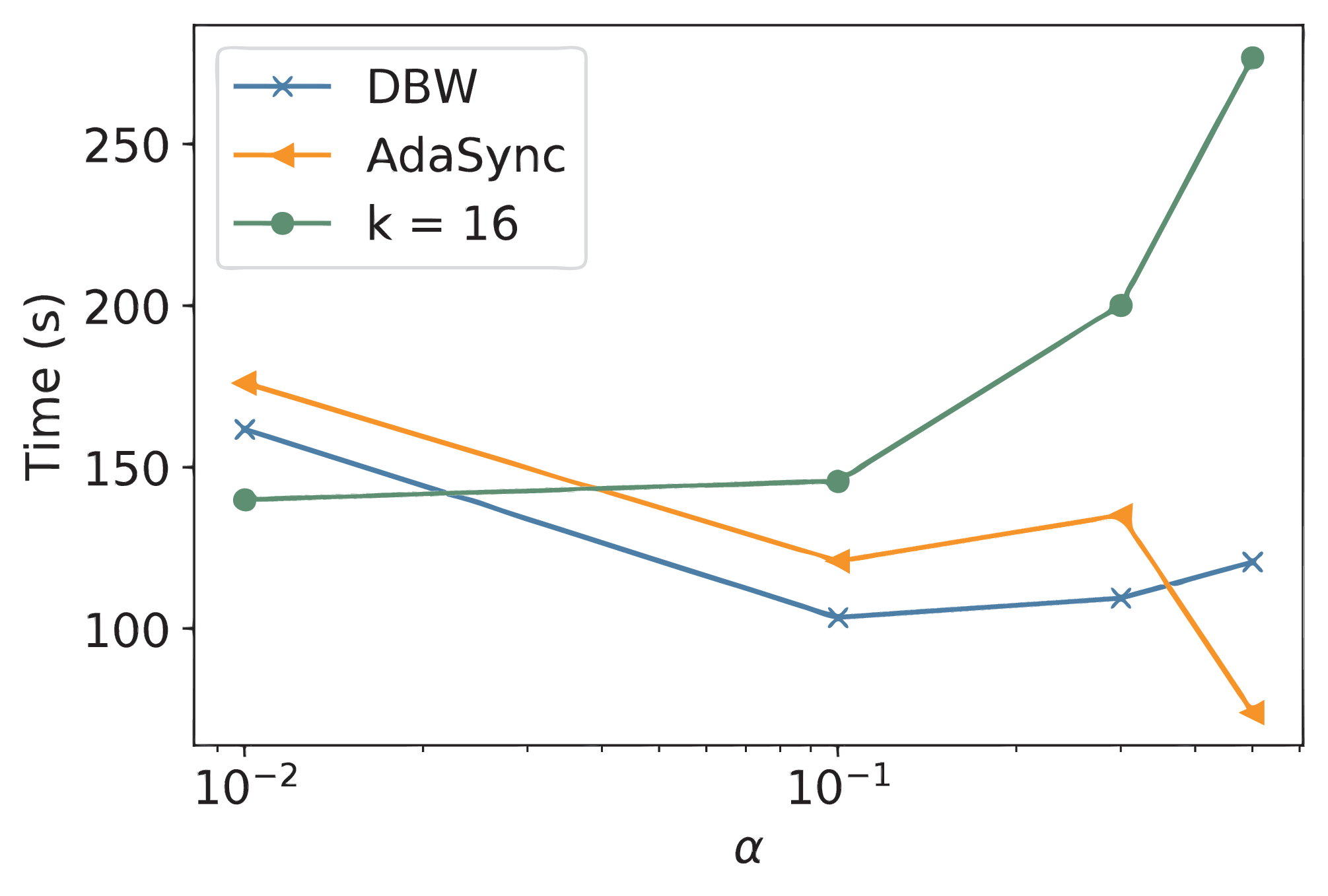
AdaSync [27] is a dynamic backup scheme designed for the Push and Interrupt (PsI) case, under the assumption that the round trip times follow shifted exponential distribution. For the comparison, we consider then this setting. For AdaSync, the quadratic formulation in [27, Appendix D.1] is used to derive the number of backup workers. AdaSync updates $k$ at the end of a time-window. We consider this time-window small enough for AdaSync evaluating the possibility to update $k_{t}$ at each iteration, as DBW does.

Figure 10(a) shows, for a single run of the training process, the evolution of the loss over time and the corresponding choices of $k_{t}$ for DBW and AdaSync, when $\alpha=0.1$, i.e., round trip times follow distribution $0.9+0.1\textrm{Exp}(1)$. DBW quickly reaches a large value of $k_{t}$ close to $n$. For small $\alpha$ the variance of round trip time is small, so choosing large $k_{t}$ does not lead large iteration times $\mathbb{E}[T_{k,t}]$ but benefits the gain in (9). The approximated formula used by AdaSync, even if derived under the assumption of shifted exponential distributions, does not depend on $\alpha$, and AdaSync fails to increase fast the value of $k_{t}$.

Fig. 10(b) shows the average convergence time⁸⁸ 8 The convergence time noted here is the time when the training loss reaches 0.07. computed over 10 independent runs under different $\alpha$. The larger $\alpha$, the larger the variance of round trip times. We can see that when $\alpha$ is smaller than 0.3, DBW performs better than AdaSync. While, AdaSync works better for larger $\alpha$, which suggests DBW may be too conservative on the number of backup workers in the late phase of the training.

Remember that the estimated gain $\widehat{\mathcal{G}_{k,t}}$ used in (18) for choosing $k_{t}$, is a lower bound for the true loss decrease. In the late training phase, when the gradient norm becomes smaller, small values of $k$ may lead to estimate a negative (see (16)). In this case, DBW conservatively chooses a larger $k$ for which the gain is estimated to be positive. On the other hand, AdaSync requires prior knowledge on the round trip time distribution. This distribution may be hard to estimate and may change during the training period, that is often very long for state-of-the-art machine learning models (e.g., weeks). Notice that DBW does not require any prior knowledge on the system.

References

- [1] K. Canini, T. Chandra, E. Ie, J. McFadden, K. Goldman, M. Gunter, J. Harmsen, K. LeFevre, D. Lepikhin, T. Lloret Llinares, I. Mukherjee, F. Pereira, J. Redstone, T. Shaked, Y. Singer, Sibyl: A system for large scale supervised machine learning, Tech. talk (2014).
- [2] E. P. Xing, Q. Ho, P. Xie, D. Wei, Strategies and principles of distributed machine learning on big data, Engineering 2 (2) (2016) 179 – 195.
- [3] A. Harlap, H. Cui, W. Dai, J. Wei, G. R. Ganger, P. B. Gibbons, G. A. Gibson, E. P. Xing, Addressing the straggler problem for iterative convergent parallel ML, in: Proceedings of the Seventh ACM Symposium on Cloud Computing, SoCC ’16, ACM, New York, NY, USA, 2016, pp. 98–111.
- [4] H. Wang, D. Niu, B. Li, Distributed machine learning with a serverless architecture, in: IEEE INFOCOM 2019 - IEEE Conference on Computer Communications, 2019, pp. 1288–1296.
- [5] Z. Shi, A. Eryilmaz, A flexible distributed optimization framework for service of concurrent tasks in processing networks, in: IEEE INFOCOM 2019 - IEEE Conference on Computer Communications, 2019, pp. 1072–1080.
- [6] Y. Bao, Y. Peng, C. Wu, Deep learning-based job placement in distributed machine learning clusters, in: IEEE INFOCOM 2019 - IEEE Conference on Computer Communications, 2019, pp. 505–513.
- [7] C. Chen, W. Wang, B. Li, Round-robin synchronization: Mitigating communication bottlenecks in parameter servers, in: IEEE INFOCOM 2019 - IEEE Conference on Computer Communications, 2019, pp. 532–540.
- [8] S. Shi, X. Chu, B. Li, Mg-wfbp: Efficient data communication for distributed synchronous SGD algorithms, in: IEEE INFOCOM 2019 - IEEE Conference on Computer Communications, 2019, pp. 172–180.
- [9] X. Zhang, J. Wang, G. Joshi, C. Joe-Wong, Machine learning on volatile instances, in: IEEE INFOCOM 2020 - IEEE Conference on Computer Communications, 2020, pp. 139–148. doi:10.1109/INFOCOM41043.2020.9155448.
- [10] M. Li, D. G. Andersen, J. W. Park, A. J. Smola, A. Ahmed, V. Josifovski, J. Long, E. J. Shekita, B.-Y. Su, Scaling distributed machine learning with the parameter server, in: Proceedings of the 11th USENIX Conference on Operating Systems Design and Implementation, 2014, pp. 583–598.
- [11]
P. Patarasuk, X. Yuan,
Bandwidth optimal
all-reduce algorithms for clusters of workstations, J. Parallel Distributed
Comput. 69 (2) (2009) 117–124.
doi:10.1016/j.jpdc.2008.09.002.
URL https://doi.org/10.1016/j.jpdc.2008.09.002 - [12]
S. Jeaugey,
Massively
scale your deep learningtraining with nccl 2.4. (2019).
URL https://developer.nvidia.com/blog/massively-scale-deep-learning-training-nccl-2-4/ - [13] MPI (https://www.mpich.org/static/docs/v3.1/www3/MPI_Allreduce.html).
- [14] A. Gibiansky, Bringing hpc techniques to deep learning (2017).
- [15] J. Dean, L. A. Barroso, The tail at scale, Communications of the ACM 56 (2) (2013) 74–80.
- [16] G. Ananthanarayanan, A. Ghodsi, S. Shenker, I. Stoica, Effective straggler mitigation: Attack of the clones, in: Proc. of the 10th USENIX Conf. NSDI, 2013, pp. 185–198.
- [17] C. Karakus, Y. Sun, S. Diggavi, W. Yin, Straggler mitigation in distributed optimization through data encoding, in: Proc. of NIPS, 2017, pp. 5434–5442.
- [18] S. Li, S. M. M. Kalan, A. S. Avestimehr, M. Soltanolkotabi, Near-optimal straggler mitigation for distributed gradient methods, in: IEEE International Parallel and Distributed Processing Symposium Workshops, 2018, pp. 857–866.
- [19]
A. Reisizadeh, S. Prakash, R. Pedarsani, A. S. Avestimehr,
Codedreduce: A fast and robust
framework for gradient aggregation in distributed learning, CoRR
abs/1902.01981 (2019).
arXiv:1902.01981.
URL http://arxiv.org/abs/1902.01981 - [20]
R. Tandon, Q. Lei, A. G. Dimakis, N. Karampatziakis,
Gradient coding:
Avoiding stragglers in distributed learning, Vol. 70 of Proceedings of
Machine Learning Research, PMLR, International Convention Centre, Sydney,
Australia, 2017, pp. 3368–3376.
URL http://proceedings.mlr.press/v70/tandon17a.html - [21] K. Lee, M. Lam, R. Pedarsani, D. Papailiopoulos, K. Ramchandran, Speeding up distributed machine learning using codes, IEEE Transactions on Information Theory 64 (3) (2017) 1514–1529.
- [22]
W. Halbawi, N. A. Ruhi, F. Salehi, B. Hassibi,
Improving distributed
gradient descent using reed-solomon codes, in: 2018 IEEE International
Symposium on Information Theory, ISIT 2018, Vail, CO, USA, June 17-22,
2018, IEEE, 2018, pp. 2027–2031.
doi:10.1109/ISIT.2018.8437467.
URL https://doi.org/10.1109/ISIT.2018.8437467 - [23]
Q. Yu, S. Li, N. Raviv, S. M. M. Kalan, M. Soltanolkotabi, S. A. Avestimehr,
Lagrange coded computing:
Optimal design for resiliency, security, and privacy, Vol. 89 of Proceedings
of Machine Learning Research, PMLR, 2019, pp. 1215–1225.
URL http://proceedings.mlr.press/v89/yu19b.html - [24] A. Reisizadeh, S. Prakash, R. Pedarsani, A. S. Avestimehr, Coded computation over heterogeneous clusters, IEEE Transactions on Information Theory 65 (7) (2019) 4227–4242.
- [25] E. Ozfatura, S. Ulukus, D. Gündüz, Straggler-aware distributed learning: Communication–computation latency trade-off, Entropy 22 (5) (2020) 544.
- [26] A. Reisizadeh, S. Prakash, R. Pedarsani, A. S. Avestimehr, Tree gradient coding, in: 2019 IEEE International Symposium on Information Theory (ISIT), IEEE, 2019, pp. 2808–2812.
- [27] S. Dutta, J. Wang, G. Joshi, Slow and stale gradients can win the race (2020). arXiv:arXiv:2003.10579.
- [28] B. McMahan, E. Moore, D. Ramage, S. Hampson, B. A. y Arcas, Communication-efficient learning of deep networks from decentralized data, in: Artificial Intelligence and Statistics, PMLR, 2017, pp. 1273–1282.
- [29] Y. Peng, Y. Bao, Y. Chen, C. Wu, C. Guo, Optimus: an efficient dynamic resource scheduler for deep learning clusters, in: Proceedings of the Thirteenth EuroSys Conference, 2018, pp. 1–14.
- [30] J. Cipar, Q. Ho, J. K. Kim, S. Lee, G. R. Ganger, G. Gibson, K. Keeton, E. Xing, Solving the straggler problem with bounded staleness, in: Presented as part of the 14th Workshop on Hot Topics in Operating Systems, 2013.
- [31] S. Dutta, G. Joshi, S. Ghosh, P. Dube, P. Nagpurkar, Slow and stale gradients can win the race: Error-runtime trade-offs in distributed SGD, AISTATS (2018).
- [32] W. Dai, Y. Zhou, N. Dong, H. Zhang, E. P. Xing, Toward understanding the impact of staleness in distributed machine learning, in: 7th International Conference on Learning Representations, ICLR 2019, 2019.
- [33] A. Nedic, A. Ozdaglar, Distributed subgradient methods for multi-agent optimization, IEEE Transactions on Automatic Control 54 (1) (2009) 48–61.
- [34] J. C. Duchi, A. Agarwal, M. J. Wainwright, Dual averaging for distributed optimization: Convergence analysis and network scaling, IEEE Trans. on Automatic Control 57 (3) (2012) 592–606.
- [35] X. Lian, C. Zhang, H. Zhang, C. Hsieh, W. Zhang, J. Liu, Can decentralized algorithms outperform centralized algorithms? A case study for decentralized parallel stochastic gradient descent, in: Advances in Neural Information Processing Systems 30: Annual Conference on Neural Information Processing Systems 2017, 2017, pp. 5330–5340.
- [36] A. Elgabli, J. Park, A. S. Bedi, M. Bennis, V. Aggarwal, Gadmm: Fast and communication efficient framework for distributed machine learning., Journal of Machine Learning Research 21 (76) (2020) 1–39.
- [37] G. Neglia, G. Calbi, D. Towsley, G. Vardoyan, The role of network topology for distributed machine learning, in: IEEE INFOCOM 2019 - IEEE Conference on Computer Communications, 2019, pp. 2350–2358.
- [38] G. Neglia, C. Xu, D. Towsley, G. Calbi, Decentralized gradient methods: does topology matter?, Vol. 108 of Proceedings of Machine Learning Research, PMLR, 2020, pp. 2348–2358.
- [39] O. Marfoq, C. Xu, G. Neglia, R. Vidal, Throughput-optimal topology design for cross-silo federated learning, in: Advances in Neural Information Processing Systems (NeurIPS), 2020.
- [40] J. Chen, R. Monga, S. Bengio, R. Jozefowicz, Revisiting distributed synchronous SGD, in: International Conference on Learning Representations Workshop Track, 2016.
- [41]
C. Xu, G. Neglia, N. Sebastianelli,
Dynamic backup workers
for parallel machine learning, in: 2020 IFIP Networking Conference,
Networking 2020, Paris, France, June 22-26, 2020, IEEE, 2020, pp. 574–578.
URL https://ieeexplore.ieee.org/document/9142724 - [42] DBW, https://gitlab.inria.fr/chxu/dbw.
- [43] TensorFlow (https://www.tensorflow.org/).
- [44] M. Teng, F. Wood, Bayesian distributed stochastic gradient descent, in: Advances in Neural Information Processing Systems 31, 2018, pp. 6378–6388.
- [45] Y. Ling, T. Mullen, X. Lin, Analysis of optimal thread pool size, SIGOPS Oper. Syst. Rev. 34 (2) (2000) 42–55.
- [46] M. M. Amiri, D. Gündüz, Computation scheduling for distributed machine learning with straggling workers, in: IEEE International Conference on Acoustics, Speech and Signal Processing, ICASSP 2019, 2019, pp. 8177–8181.
- [47] Q. Luo, J. Lin, Y. Zhuo, X. Qian, Hop: Heterogeneity-aware decentralized training, in: Proceedings of the Twenty-Fourth International Conference on Architectural Support for Programming Languages and Operating Systems, 2019, pp. 893–907.
- [48] PyTorch (https://pytorch.org/).
- [49] L. Balles, J. Romero, P. Hennig, Coupling adaptive batch sizes with learning rates, in: Proc. of the Thirty-Third Conference on Uncertainty in Artificial Intelligence (UAI), 2017.
- [50] S. Bubeck, Convex optimization: Algorithms and complexity, Found. Trends Mach. Learn. 8 (3-4) (2015) 231–357.
- [51] L. Bottou, F. E. Curtis, J. Nocedal, Optimization methods for large-scale machine learning, Siam Review 60 (2) (2018) 223–311.
- [52]
G. Neglia, C. Xu, D. Towsley, G. Calbi,
Decentralized
gradient methods: does topology matter?, in: S. Chiappa, R. Calandra (Eds.),
The 23rd International Conference on Artificial Intelligence and Statistics,
AISTATS 2020, 26-28 August 2020, Online [Palermo, Sicily, Italy], Vol. 108
of Proceedings of Machine Learning Research, PMLR, 2020, pp. 2348–2358.
URL http://proceedings.mlr.press/v108/neglia20a.html - [53] K. Lee, M. Lam, R. Pedarsani, D. Papailiopoulos, K. Ramchandran, Speeding up distributed machine learning using codes, IEEE Transactions on Information Theory 64 (3) (2018) 1514–1529.
- [54] M. Grant, S. Boyd, CVX: Matlab software for disciplined convex programming, version 2.1 (Mar. http://cvxr.com/cvx, 2014).
- [55] M. Grant, S. Boyd, Graph implementations for nonsmooth convex programs, in: Recent Advances in Learning and Control, Lecture Notes in Control and Information Sciences, Springer-Verlag Limited, 2008, pp. 95–110.
- [56] S. De, A. Yadav, D. Jacobs, T. Goldstein, Automated inference with adaptive batches, in: Proceedings of the 20th International Conference on Artificial Intelligence and Statistics (AISTATS), 2017, pp. 1504–1513.
- [57] MNIST database (http://yann.lecun.com/exdb/mnist/).
- [58] A. Krizhevsky, G. Hinton, et al., Learning multiple layers of features from tiny images (2009).
- [59] K. He, X. Zhang, S. Ren, J. Sun, Deep residual learning for image recognition, in: Proceedings of the IEEE conference on computer vision and pattern recognition, 2016, pp. 770–778.
- [60] P. Goyal, P. Dollár, R. B. Girshick, P. Noordhuis, L. Wesolowski, A. Kyrola, A. Tulloch, Y. Jia, K. He, Accurate, large minibatch SGD: training imagenet in 1 hour, CoRR abs/1706.02677 (2017). arXiv:1706.02677.
- [61] S. L. Smith, P.-J. Kindermans, Q. V. Le, Don’t decay the learning rate, increase the batch size, in: International Conference on Learning Representations, 2018.
- [62] L. N. Smith, Cyclical learning rates for training neural networks, in: Applications of Computer Vision (WACV), 2017 IEEE Winter Conference on, IEEE, 2017, pp. 464–472.
- [63] S. Dutta, G. Joshi, S. Ghosh, P. Dube, P. Nagpurkar, Slow and stale gradients can win the race: Error-runtime trade-offs in distributed SGD, in: International Conference on Artificial Intelligence and Statistics, AISTATS 2018, 2018, pp. 803–812.
- [64] E. Hoffer, I. Hubara, D. Soudry, Train longer, generalize better: closing the generalization gap in large batch training of neural networks, in: Advances in Neural Information Processing Systems 30, Curran Associates, Inc., 2017, pp. 1731–1741.
- [65] F. Pace, D. Venzano, D. Carra, P. Michiardi, Flexible scheduling of distributed analytic applications, CCGrid ’17, IEEE Press, 2017, pp. 100–109.
- [66] F. P. Kelly, A. K. Maulloo, D. K. Tan, Rate control for communication networks: shadow prices, proportional fairness and stability, Journal of the Operational Research society 49 (3) (1998) 237–252.
- [67] J. Konecný, B. McMahan, D. Ramage, Federated optimization: Distributed optimization beyond the datacenter, in: Neural Information Processing Systems (workshop), 2015.