Deconfined Metal-Insulator Transitions in Quantum Hall Bilayers

Introduction. Understanding quantum criticality in metallic systems remains one of the outstanding challenges in the study of quantum matter, largely due to the abundance of gapless excitations near the electronic Fermi surface (FS). Describing an interaction-driven continuous metal-insulator transition is especially challenging, and a mechanism for an abrupt change of a generic electronic FS (at a fixed electron density) across a transition to an insulator in the absence of disorder is necessarily novel. Critical theories for continuous metal-insulator transitions, involving the disappearance of an entire electronic FS, have been formulated when the insulator is a quantum spin liquid with a FS of neutral excitations (e.g., “spinons”) coupled to emergent gauge fields Senthil et al. 2004; Senthil 2008a. Pressure-tuned experiments on certain spin liquid candidates Kanoda and Kato 2011 have reported indirect evidence for such a transition Furukawa et al. 2015. One of the most challenging and unsolved problems in the field is to describe a continuous metal-insulator transition where the insulator has no remnant FS of any excitations, which we dub a “Deconfined Metal-Insulator Transition” (DMIT), or a Deconfined Mott Transition in the terminology of Ref. Zou and Chowdhury 2020. Such a transition necessarily falls outside the purview of the conventional Landau-Ginzburg-Wilson paradigm, even though the phases on either side of the transition can be conventional. Finding concrete theoretical examples of a DMIT in a solvable limit is therefore of paramount importance.

There are indirect signatures of continuous transitions between distinct metallic phases in numerous systems. For instance, in certain rare-earth element based (“heavy-fermion”) compounds there is evidence for entire Fermi surface sheets disappearing Stewart 2001; Schröder et al. 2000, accompanied by a diverging effective mass near the putative critical point Shishido et al. 2005. Perhaps the most notable example of a similar transition arises in the cuprate superconductors Keimer et al. 2015, where a Fermi liquid (FL) metal evolves into an unconventional “pseudogap” metal Badoux et al. 2016. It is important to note that none of these transitions can be described by the conventional framework of coupling an order-parameter field to an electronic FS. Recently, we have argued that the DMIT can be used as a building block to describe such experimentally relevant continuous transitions between distinct metallic phases, simply by including additional spectator electrons in the low-energy description that do not alter any fundamental aspects of the criticality itself Zou and Chowdhury 2020.

A general mechanism for DMIT based on “emergent color superconductivity” Alford et al. 2008 was proposed in Ref. Zou and Chowdhury 2020. In this work, inspired by the recent experimental advances in realizing quantum Hall (QH) physics in the presence of a periodic potential at the scale of the magnetic length (e.g., in moiré heterostructures) Hunt et al. 2013; Ponomarenko et al. 2013; Dean et al. 2013; Spanton et al. 2018, we theoretically study a concrete setting for DMIT.

Setup and framework. Consider a QH bilayer separated by a distance, $d$, with a periodic potential in each layer (Fig. 1); we will refer to this setup as a “Chern bilayer”. To be concrete, we fix a unit flux quantum threading through each unit cell (UC) of the periodic potential. We will consider spinful electrons in each layer, such that spin-up electrons in the $S^{z}$-basis have a fixed density $\nu_{\uparrow}=2+\nu$ with $\nu=C/(C+1)$ per UC per layer ($C\in$ integer; $C\neq 0,-1$), while spin-down electrons have a fixed density $\nu_{\downarrow}=1$ per UC per layer. We will focus on $C>0$, but the phenomenology will be similar when $C<0$. We further assume that the electron number in each layer is conserved¹¹ 1 This assumption on particle number conservation in each layer can be relaxed, as long as the total particle number is conserved., the total $S^{z}$-spin is conserved, and the system is symmetric with respect to exchanging the two layers and with respect to an inversion within each layer. We are interested in the situation where the electrons interact via a repulsive two-body long-range density-density interaction $V(r)\sim 1/r^{1+\epsilon}$, with $r$ denoting the (three-dimensional) separation. The case with $\epsilon=0$ corresponds to Coulomb repulsion. We focus on $0<\epsilon<1$ for most of our discussion, and comment on the cases of $\epsilon=0$ and $\epsilon\geqslant 1$ at the end. We stress that the condition $0<\epsilon<1$ is introduced purely for technical convenience, and it should not be viewed as a fundamental limitation of our proposal.

An equivalent description of this system is to view each layer as being made of spin-up electrons with fixed density $\nu^{\prime}=1+\nu$ and spinless Cooper pairs with fixed density $\nu_{B}=1$. Below we will adopt this view since it is more convenient for our purpose. So each layer has “valence” (spin-up) electrons at a density of 1 per UC, and “conduction” (spin-up) electrons at a density of $\nu$. In fact, we will consider a scenario where the actions associated with the transitions mostly take place in the conduction electrons, while the valence electrons and Cooper pairs are gapped spectators that are coupled in a special way to enable the transitions to be direct. Our proposal will thus serve as a proof-of-concept setup for realizing DMIT in an electronic model.

To understand the DMIT in this setup, consider a single layer first. An earlier work Barkeshli and McGreevy 2012 studied the possibility of a continuous transition between a FL and a composite Fermi liquid (CFL) of spinless electrons Halperin et al. 1993. However, it is our understanding that the resulting transition can only be accessed by tuning two parameters (instead of one) in order to avoid an intermediate phase. Interestingly, we will see that an analogous transition can be realized simply by tuning one parameter for the spinful electrons discussed above. Building on this idea and the recent results of Ref. Lee et al. 2018 on transitions between distinct fractional Chern insulators, we can describe a continuous transition between a FL and a to-be-introduced “generalized” CFL (gCFL) in our setup (Fig. 1b); the universal critical properties can be understood in a controlled manner when $C\gg 1$. For the bilayer (Fig. 1a) coupled via the long-range repulsion, we show that the corresponding gCFL phase is unstable to an insulator without FS of any excitations Bonesteel et al. 1996; Sodemann et al. 2017; Isobe and Fu 2017; sup 2020. Moreover, when $C\gg 1$, we will show that the couplings between the two layers are renormalization-group (RG) irrelevant at the FL-gCFL transition. Therefore, our Chern bilayer hosts an example of a DMIT (Fig. 1c), where each layer undergoes a FL-gCFL transition (the latter being unstable to an insulator). Furthermore, the critical point hosts a non-Fermi liquid (nFL) with a sharply defined critical FS Senthil 2008b.

More specifically, denote the annihilation operator of spin-up electrons and spinless Cooper pairs on the $\ell$-th layer by $c_{\ell}$ and $B_{\ell}$, respectively. We express $c_{\ell}$ in terms of partons as $c_{\ell}=b_{\ell}f_{\ell}$, where $b_{\ell}$ and $f_{\ell}$ are bosonic and fermionic partons, respectively, that satisfy a constraint on their densities Wen 2004, $n_{b_{\ell}}=n_{f_{\ell}}=\nu^{\prime}$. The low-energy theory for this parton construction of the spin-up electrons can be written in terms of the partons coupled to an emergent dynamical U$(1)$ gauge field, $a_{\ell}$. We let $b_{\ell}$ carry the global conserved U$(1)$ charge associated with the $\ell$-th layer and $f_{\ell}$ carry the spin (see Table 1), such that the schematic Lagrangian for the $\ell$-th layer takes the form:

where $A_{\ell}$ and $A_{s}$ are the probe gauge fields corresponding to the conserved charge on the $\ell$-th layer and total $S^{z}$-spin, respectively. The interlayer couplings will be discussed later. In the remainder of this paper we will take $\mathcal{L}_{\ell}$ to yield no net flux for $a_{\ell}$ and to describe a FS of $f_{\ell}$ at the mean-field level; we tune $\mathcal{L}_{[b_{\ell},A_{\ell}-a_{\ell}]}$ to drive the transition.

One may wonder whether it requires fine-tuning to fix the flux of $a_{\ell}$ at the transition. We will see that in our setup the coupling between valence spin-up electrons and Cooper pairs, chosen as $\mathcal{L}_{[c_{\ell},B_{\ell}]}=-\frac{2}{2\pi}A_{\ell}d(A_{\ell}-a_{\ell})$, can fix the flux of $a_{\ell}$ without any fine-tuning. So below we will assume that $a_{\ell}$ has no net flux and focus on the conduction spin-up electrons. Later we will elaborate on the role of the gapped spectator valence electrons and Cooper pairs.

Before describing our results for the Chern bilayer in detail, we outline some key features associated with the phases and transitions of interest (see Fig. 2). By tuning a single parameter (denoted $m$ in Eq. (2)), the bosonic partons can be driven from a superfluid (SF) to a QH state. In terms of electrons, the SF corresponds to a FL, and the SF condensate fraction determines the quasiparticle-residue, $Z$ (i.e., the overlap between the electronic quasiparticle and the microscopic electron), which vanishes continuously upon approaching the DMIT. The boson gap, $\Delta_{b}$, opens up continuously on the QH side, where the latter corresponds to a gCFL in terms of electrons. One of the highlights of the present work is to identify a mechanism whereby, in the bilayer setting, the interlayer pairing of $f_{\ell}$ is dangerously irrelevant, leading to a continuous opening of the fermionic gap, $\Delta_{f}$. Remarkably, all three quantities vanish at the critical point, which hosts a sharply defined FS without any long-lived quasiparticles.

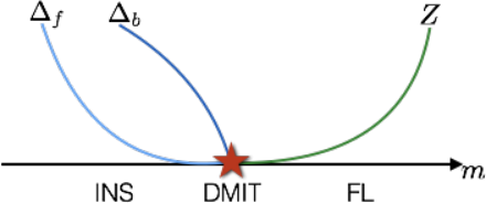
Single-layer physics. Consider a transition between a SF and a QH state for $b_{\ell}$, with the critical theory given by Barkeshli and McGreevy 2014; Lee et al. 2018; sup 2020

where $ada\equiv\epsilon_{\mu\nu\lambda}a_{\mu}\partial_{\nu}a_{\lambda}$, ${\rm{CS}}_{g}$ is a gravitational Chern-Simons (CS) term Zou and He 2020, and ${\not{D}}_{\alpha_{\ell}}$ is the covariant derivative with respect to a new emergent gauge field, $\alpha_{\ell}$. In this theory, $b_{\ell}^{\dagger}$ is the monopole of $\alpha_{\ell}$ and the density fluctuations of $b_{\ell}$ correspond to the flux of $\alpha_{\ell}$; the transition is then driven by tuning the mass, $m$, of $(C+1)$ flavors of emergent Dirac fermions, $\psi_{\ell i}$. ²² 2 In terms of the flux-attachment picture, the first term in Eq. (2) attaches one flux quantum to each boson $b_{\ell}$ and converts it into a fermion, $\psi_{\ell}$, which thereby sees a net flux of $1-\nu=\frac{1}{C+1}$ per UC. The phase transition corresponds to one where the Chern number of $\psi_{\ell}$ changes from $-1$ to $C$, which is captured Lee et al. 2018 by the last three terms in Eq. (2). An alternative derivation for Eq. (2) appears in sup 2020.

What are the different phases that the theory given by (1) and (2) can describe by varying $m$? When $m>0$, for any $C$, integrating $\psi_{\ell i}$ out removes the CS term of $\alpha_{\ell}$ and the resulting state is a SF of $b_{\ell}$, as is evident from the Dasgupta-Halperin duality Dasgupta and Halperin 1981. In terms of the original $c_{\ell}$, this is just a FL phase when $f_{\ell}$ forms a FS. ³³ 3 When discussing the various phases, we have assumed that the valence part of $f_{\ell}$ has no Chern number. It is straightforward to generalize the discussion to the case where it has a Chern number. Notice that the universal critical physics at the transitions does not depend on this Chern number. On the other hand, when $m<0$, integrating $\psi_{\ell i}$ out leads to

which is a QH state of $b_{\ell}$. When $f_{\ell}$ forms a FS, the resulting state of the original $c_{\ell}$ is a gCFL sup 2020. Indeed, upon further integrating out the gapped $\alpha_{\ell}$, the effective theory reduces to

When $C=1$ and ignoring $\mathcal{L}_{[c_{\ell},B_{\ell}]}$, this is precisely the effective theory of the familiar CFL at $\nu=1/2$, which hosts a nFL of $f_{\ell}$ Halperin et al. 1993. When $C\in$ integers ($\neq 0,\pm 1$), the qualitative picture for the universal physics associated with $(f_{\ell},a_{\ell})$ largely remains the same, in that the thermodynamic and transport properties of the gCFL are similar to the usual CFL, while the spectral properties are qualitatively different sup 2020.

Next we turn to the critical point in Eq. (2), and ignore its coupling to the $(f_{\ell},a_{\ell})$-sector (and the spectator-sector). An important observation is that, for any $C$, the magnetic translation symmetry forbids various potentially relevant perturbations at this transition, such that the transition can be accessed by tuning a single parameter, $m$ Lee et al. 2018. When $C\gg 1$, this theory can be studied in a controlled manner, and it flows in the IR to a conformal field theory (CFT) Chen et al. 1993. As shown in Fig. 2 (but for the single-layer problem), $Z\sim|\langle b_{\ell}\rangle|^{2}$ and $\Delta_{b}$ vanish continuously as we approach the transition from the superfluid and QH side, respectively; $\Delta_{f}=0$ in the present single-layer setup.

Note that the long-range interaction $V(r)$ is not included above, which takes the form (in the Coulomb gauge with $\bm{\nabla}\cdot\bm{\alpha}_{\ell}=0$),

with $\alpha_{\ell t}$ the transverse spatial component of $\alpha_{\ell}$ Halperin et al. 1993. When $\epsilon>0$, this interaction is irrelevant compared to the CS term of $\alpha_{\ell}$, so it can be ignored at the critical point. In passing, we note that a Maxwell term for $\alpha_{\ell}$ is invariably generated due to local interactions, which is less (equally or more) relevant than (5) if $\epsilon<1$ ($\epsilon\geqslant 1$). So this long-range interaction is important if $\epsilon<1$, while if $\epsilon\geqslant 1$, we can ignore it and consider only local interactions as far as universal critical physics is concerned.

Now we need to combine the $b_{\ell}$-sector and the $(f_{\ell},a_{\ell})$-sector, which are coupled via operators of the form $\mathcal{O}_{b_{\ell}}\mathcal{O}_{(f_{\ell},a_{\ell})}$, where $\mathcal{O}_{b_{\ell}}$ and $\mathcal{O}_{(f_{\ell},a_{\ell})}$ are gauge invariant operators from the two sectors, respectively. Naively, as long as the scaling dimensions of these operators are large enough, such couplings are RG irrelevant and the two sectors are effectively decoupled. Indeed, as pointed out in Ref. Senthil 2008a, when the scaling dimensions of all gauge invariant operators in the $b_{\ell}$-sector are larger than $3/2$, the criticality of $b_{\ell}$ is unaffected by the presence of the $(f_{\ell},a_{\ell})$-sector. When $C\gg 1$, this condition is satisfied for the CFT corresponding to (2) Chen et al. 1993. However, the presence of the critical $b_{\ell}$-sector has a significant influence on the dynamics of the $(f_{\ell},a_{\ell})$-sector. In particular, integrating out $b_{\ell}$ at the critical point generates the following effective action for $a_{\ell}$:

with $\sigma_{b}$ a universal constant determined by the CFT corresponding to (2), $a_{\ell t}$ the transverse spatial component of $a_{\ell}$, and the boson velocity is set to unity. As a result of Landau-damping due to coupling to the FS of $f_{\ell}$, the effective action for $a_{\ell t}$ has an additional contribution, $\int_{\omega,\bm{k}}\frac{|\omega|}{k}|a_{\ell t}(\bm{k},\omega)|^{2}$, leading to a dynamical exponent $z_{a}=2$. As a result, at the critical point, the $f_{\ell}$ are endowed with a marginal FL-like self-energy and the electrons have a well-defined critical FS without long-lived quasiparticles.

Finally, we examine the important and subtle issue of the flux of $a_{\ell}$ and the role of the spectator valence electrons and Cooper pairs. If there is no nontrivial coupling $\mathcal{L}_{[c_{\ell},B_{\ell}]}$ in (1), nothing fixes this flux at the transition. So without fine-tuning, a net flux of $a_{\ell}$ can be generated and the critical point is expected to be unstable to forming certain QH state. However, unlike earlier approaches Barkeshli and McGreevy 2012, this aspect can be circumvented by incorporating a nontrivial $\mathcal{L}_{[c_{\ell},B_{\ell}]}$. Specifically, denote the valence part of $b_{\ell}$ by $b_{\ell v}$, and attach a vortex of $B_{\ell}$ to $b_{\ell,v}$, and a vortex of $b_{\ell,v}$ to $B_{\ell}$. This coupling induces an interaction $\mathcal{L}_{[c_{\ell},B_{\ell}]}=-\frac{2}{2\pi}A_{\ell}d(A_{\ell}-a_{\ell})$ at low energies Senthil and Levin 2013, which means the flux of $a_{\ell}$ now carries charge under $A_{\ell}$. Because the charge under $A_{\ell}$ is fixed, now the flux of $a_{\ell}$ is also fixed (without fine-tuning) sup 2020.

DMIT in bilayer. When the two identical layers with separately conserved densities are coupled through the long-range repulsion, we obtain two effectively decoupled FL for $m>0$. What is the fate of the system when $m<0$?

A useful starting point is to consider the limit where the two layers are completely decoupled so that each of them can be captured within the above discussion, and then study the effect of interlayer couplings as we tune through the individual single-layer FL-gCFL transition. This scenario can be physically realized when $d$ is large.

We begin by introducing $a_{\pm}\equiv(a_{1}\pm a_{2})/2$, where the layer-exchange symmetry forbids a direct coupling between $a_{+}$ and $a_{-}$. As argued in Refs. Bonesteel et al. 1996; Zou and Senthil 2016; Sodemann et al. 2017; Isobe and Fu 2017; Zou and Chowdhury 2020, $a_{+}$ tends to suppress pairing of the FS while $a_{-}$ favors interlayer pairing, such that their competition determines the stability of the FS. When $b_{\ell}$ is gapped, (4) indicates that the density fluctuation of $f_{\ell}$ is related to the flux of $a_{\ell}$, so the long-range repulsion becomes an interaction between flux of $a_{\pm}$. Notice that $a_{+}$ couples to the total density of $f_{1}$ and $f_{2}$, while $a_{-}$ couples to the density difference between $f_{1}$ and $f_{2}$. So the flux of $a_{+}$ experiences the long-range potential, while the interaction between the flux of $a_{-}$ is effectively short-ranged. As a result, the coupling between $a_{-}$ and the fermions is more relevant and the FS is unstable to interlayer pairing sup 2020. This implies that two layers of gCFL are unstable to forming an insulating phase and we discuss its topological character shortly. Since the boson gap, $\Delta_{b}$, serves as the effective UV cutoff of the low-energy physics associated with the interlayer pairing, the resulting pairing gap, $\Delta_{f}$, should be smaller than $\Delta_{b}$ (see Fig. 2).

At the critical point, we should instead use the effective action in (6) to describe the gauge fields and determine the stability of the FS. Rewriting

with $a_{\pm t}$ the transverse spatial component of $a_{\pm}$, we can identify the gauge couplings $g_{+}=g_{-}=1/(4\sigma_{b})$. When $z_{a}=2$, the FS is perturbatively stable if $g_{+}\geqslant g_{-}$ Zou and Chowdhury 2020.⁴⁴ 4 Kohn-Luttinger type effects Kohn and Luttinger 1965; Shankar 1994 are ignored. Therefore, interlayer pairing is (dangerously) irrelevant at this transition.

Can other interlayer couplings alter the critical properties? First, just as in the case of the monolayer, the interlayer long-range interaction is irrelevant at the critical point if $\epsilon>0$. In addition, there are local interactions that all turn out to be irrelevant Zou and Senthil 2016; sup 2020. For example, there can be a coupling of the form $\mathcal{O}_{b_{1}}\mathcal{O}^{\prime}_{b_{2}}$, where $\mathcal{O}$ and $\mathcal{O}^{\prime}$ are gauge invariant operators in the $b_{1}$- and $b_{2}$-sector, respectively. Clearly this coupling is irrelevant if the scaling dimensions of $\mathcal{O}$ and $\mathcal{O}^{\prime}$ are larger than $3/2$. In fact, a sufficient condition for the layer decoupling is that all gauge invariant operators of the $b_{\ell}$-sector have a scaling dimension larger than $3/2$ sup 2020, a condition satisfied when $C\gg 1$ Chen et al. 1993.⁵⁵ 5 Although we mainly focus on the case where the particle density in each layer is separately conserved, our conclusions regarding the interlayer pairing instability of $f$ and the DMIT are robust even in the presence of a weak interlayer electron tunneling, which leads to a single conserved U(1) density, and is irrelevant at the DMIT sup 2020.

We have thus reached the remarkable conclusion that the above bilayer setup can exhibit a DMIT, where the critical point hosts two effectively decoupled, sharp critical FS.

Topological properties of the insulating phase. The effective theory for the insulating phase in the bilayer setting is given by $\sum_{\ell}\mathcal{L}_{\ell}$ in (1), with $\mathcal{L}_{[b_{\ell},A_{\ell}-a_{\ell}]}$ given by (3), $\mathcal{L}_{[f,a+A_{s}]}$ the effective Lagrangian for the interlayer-paired state of the fermions, and $\mathcal{L}_{[c_{\ell},B_{\ell}]}=-\frac{2}{2\pi}A_{\ell}d(A_{\ell}-a_{\ell})$. Our goal is to characterize this phase via the $K$-matrix formalism Wen 2004.

Since $\alpha_{\ell}$ in (3) is coupled to a fermion, to apply the standard $K$-matrix formalism, we introduce $C+1$ gauge fields, $\beta_{\ell}^{i}$ ($i=1,2,\cdots,C+1$) for the $\ell$-th layer, which are coupled to bosons. In terms of these new gauge fields, $\mathcal{L}_{[b_{\ell},A_{\ell}-a_{\ell}]}$ is equivalent to:

Note that integrating out $\beta_{\ell}^{i}$’s above reproduces (3). We now integrate out $\alpha_{\ell}$ and obtain a constraint

Next we turn to $\mathcal{L}_{[f,a+A_{s}]}$. The channel in which interlayer pairing occurs depends on non-universal details Bonesteel et al. 1996; Sodemann et al. 2017; Isobe and Fu 2017; sup 2020. Suppose it occurs in the channel with index $n$ in Kitaev’s 8-fold way Kitaev 2006. ⁶⁶ 6 Since our interlayer pairing is between two species of fermions, only the Abelian 8-fold way of classification is relevant here among the full 16-fold way classification of Kitaev, so we use a convention that our $n$ is half of Kitaev’s index in Ref. Kitaev 2006. The topological nature of the paired state depends on $n$, which can be described with the introduction of low-energy emergent gauge fields in addition to $a$ Kitaev 2006. Naturally, it is important to understand how these new gauge fields couple to $a_{\pm}$ and $A_{s}$.

A convenient way to proceed is to separate the charges under $a_{+}+A_{s}$ and $a_{-}$ by performing a parton decomposition of $f_{\ell}\equiv\phi d_{\ell}$, where $\phi$ is a boson such that $\phi^{2}$ is the interlayer pairing amplitude, $d_{\ell}$ is a fermion, such that $\phi$ and $d_{\ell}$ are coupled to an emergent $Z_{2}$ gauge field. Here $\phi$ carries charge $1$ under $a_{+}+A_{s}$ but no charge under $a_{-}$, and $d_{1}$ and $d_{2}$ carry charge 1 and $-1$ under $a_{-}$, respectively, but are neutral under $a_{+}+A_{s}$. In the interlayer-paired state of $f_{\ell}$, $\phi$ is condensed and $d_{\ell}$ develops interlayer pairing in the same channel as $f_{\ell}$. The condensate of $\phi$ can be captured by $\frac{1}{\pi}(a_{+}+A_{s})d\beta$, where $\beta$ is a new emergent gauge field and its elementary charge binds the $\pi$-flux of the $Z_{2}$ gauge field. This binding is why the coefficient of $(a_{+}+A_{s})d\beta$ is $1/\pi$, not $1/(2\pi)$ Senthil and Fisher 2000.

The $d_{\ell}$-sector depends on $n$, and it is most convenient to start with the case $n=\pm 1$. It is known that when the state with $n=\pm 1$ is coupled to a dynamical $Z_{2}$ gauge field, the resulting state is U$(1)_{\pm 4}$, captured by $\mp\frac{4}{4\pi}\gamma d\gamma$, where odd charge of the new emergent gauge field $\gamma$ is identified with the $\pi$-flux of the $Z_{2}$ gauge field Kitaev 2006. This identification further constrains that $q_{\beta}=q_{\gamma}\ ({\rm mod\ }2)$, where $q_{(\cdot)}$ represents the possible charge that an excitation carries under the corresponding gauge field. Since $d_{\ell}$ is coupled to $a_{-}$, we need to determine how $\gamma$ is coupled to $a_{-}$. The layer exchange symmetry requires that they are coupled via $\frac{1}{\pi}a_{-}d\gamma$ Sodemann et al. 2017. Therefore, when $n=\pm 1$,

with a constraint $q_{\beta}=q_{\gamma}\ ({\rm mod\ }2)$. To apply the standard $K$-matrix formalism, we can solve this constraint by introducing $\tilde{\beta}\equiv\beta+\gamma$ and $\tilde{\gamma}\equiv\beta-\gamma$. The charges of $\tilde{\beta}$ and $\tilde{\gamma}$ can independently take any integer. Denote the electric and spin Hall conductivity by $\sigma_{xy}^{c}$ and $\sigma_{xy}^{s}$, respectively. Plugging (3), (10) and $\mathcal{L}_{[c_{\ell},B_{\ell}]}=-\frac{2}{2\pi}A_{\ell}d(A_{\ell}-a_{\ell})$ into $\sum_{\ell}\mathcal{L}_{\ell}$ yields $\sigma_{xy}^{c}=2\nu-8$ and $\sigma_{xy}^{s}=2\nu$.

To fully unearth the topological property, we write down the final $K$-matrix theory for $n=\pm 1$ in terms of $\tilde{a}\equiv(\beta_{1}^{1},\beta_{1}^{2},\cdots,\beta_{1}^{C+1},\beta_{2}^{1},\beta_{2}^{2},\cdots,\beta_{2}^{C+1},\tilde{\beta},\tilde{\gamma})^{T}$:

with

Here $K_{1}$ is a $(C+1)\times(C+1)$ matrix whose diagonal elements vanish while all other entries are 1, $K_{2}$ ($K_{3}$) is a $(C+1)\times 2$ matrix whose entries in the first (second) column are all 1 while all other entries vanish, and

The first $C+1$ entries of $t_{1}$ ($t_{2}$) is 2 (0). In general, the above theory describes a topological order, but when $C=1$ and $n=-1$, the resulting state has a Goldstone mode due to the spontaneous breaking of a U(1) symmetry generated by $5(Q_{1}-Q_{2})-S^{z}$, with $Q_{1,2}$ the electric charge of the two layers, respectively sup 2020.

To obtain the $K$-matrix for states with other $n\neq\pm 1$ systematically, the simplest approach may be to apply the trick in Ref. Zou and He 2020 to build up the theory from that with $n=\pm 1$ sup 2020.

Observable signatures. The DMIT can be viewed as two dynamically decoupled FL-gCFL transitions (where the gCFL-bilayer is unstable to an insulator). Therefore, some of the universal physical properties at both transitions are similar Barkeshli and McGreevy 2012; Lee et al. 2018, which include: (i) a critical FS, (ii) a singular specific heat ($\sim T\ln T$) at the transition, (iii) a jump of the electric resistivity ($\sim h/e^{2}$), (vi) an emergent SU($C+1$) symmetry where a set of power-law-decaying charge-density-wave order parameters transform in its adjoint representation. One main difference between the monolayer and bilayer systems appears in the insulating side of $b_{\ell}$, where the bilayer shows interlayer pairing of $f_{\ell}$ below certain temperature scale Bonesteel et al. 1996; Sodemann et al. 2017; Isobe and Fu 2017.

Outlook. In this work, we have primarily focused on the case of a repulsive two-body interaction, $V(r)\sim 1/r^{1+\epsilon}$, with $0<\epsilon<1$, at the DMIT. For the case of usual Coulomb repulsion ($\epsilon=0$), the interaction is marginal at the tree-level with respect to the bosonic superfluid-QH transition. We leave a detailed study on the effect of Coulomb interaction on such transitions for the future Ye and Sachdev 1998. The case with $\epsilon\geqslant 1$ may be realized with cold atoms Cooper and Dalibard 2013; Yao et al. 2013, and the physics in this case reduces to that in Ref. Zou and Chowdhury 2020. The crossovers at finite temperature out of the regimes considered here are expected to be rich and we leave a detailed study of this phenomenology for future work, along with a study of the effects of different types of disorder on these transitions. The transport properties in the quantum critical regime associated with the DMIT will likely shed interesting light on the non-Fermi liquid. It would be interesting to find concrete models for these DMIT and study them numerically. A smoking-gun signature for the DMIT in the density-density response would be a sharp “$2K_{F}$” response arising from the critical Fermi surface, in addition to the set of isolated peaks from the charge-density wave due to the emergent SU$(C+1)$ symmetry at the critical point.

Acknowledgement. We thank Zhen Bi, Inti Sodemann and especially Chong Wang for useful discussions. LZ is supported by the John Bardeen Postdoctoral Fellowship at Perimeter Institute. Research at Perimeter Institute is supported in part by the Government of Canada through the Department of Innovation, Science and Economic Development Canada and by the Province of Ontario through the Ministry of Colleges and Universities. DC is supported by faculty startup funds at Cornell University.

Supplementary Material for “Deconfined Metal-Insulator Transitions in Quantum Hall Bilayers”

This Supplementary Material contains additional details on: I. the critical theory of the transition between the quantum Hall (QH) state and superfluid of the bosons, II. some of the low-energy properties of the generalized composite Fermi liquid (gCFL) phase, III. additional details on the spectator valence electrons and Cooper pairs, IV. a discussion of the interlayer pairing instability of two layers of gCFL, V. an analysis of the effects of various interlayer couplings at the metal-insulator transition, and, VI. details of deriving the topological properties of the insulating phases.

References

- Senthil et al. (2004) T. Senthil, Matthias Vojta, and Subir Sachdev, “Weak magnetism and non-fermi liquids near heavy-fermion critical points,” Physical Review B 69 (2004).
- Senthil (2008a) T. Senthil, “Theory of a continuous Mott transition in two dimensions,” Phys. Rev. B 78, 045109 (2008a), arXiv:0804.1555 [cond-mat.str-el] .
- Kanoda and Kato (2011) Kazushi Kanoda and Reizo Kato, “Mott physics in organic conductors with triangular lattices,” Annual Review of Condensed Matter Physics 2, 167–188 (2011), https://doi.org/10.1146/annurev-conmatphys-062910-140521 .
- Furukawa et al. (2015) Tetsuya Furukawa, Kazuya Miyagawa, Hiromi Taniguchi, Reizo Kato, and Kazushi Kanoda, “Quantum criticality of mott transition in organic materials,” Nature Physics 11, 221–224 (2015).
- Zou and Chowdhury (2020) Liujun Zou and Debanjan Chowdhury, “Deconfined metallic quantum criticality: A U(2) gauge-theoretic approach,” Physical Review Research 2, 023344 (2020), arXiv:2002.02972 [cond-mat.str-el] .
- Stewart (2001) G. R. Stewart, “Non-fermi-liquid behavior in - and -electron metals,” Rev. Mod. Phys. 73, 797–855 (2001).
- Schröder et al. (2000) A. Schröder, G. Aeppli, R. Coldea, M. Adams, O. Stockert, H.v. Löhneysen, E. Bucher, R. Ramazashvili, and P. Coleman, “Onset of antiferromagnetism in heavy-fermion metals,” Nature 407, 351–355 (2000).
- Shishido et al. (2005) Hiroaki Shishido, Rikio Settai, Hisatomo Harima, and Yoshichika Ōnuki, “A drastic change of the fermi surface at a critical pressure in cerhin5: dhva study under pressure,” Journal of the Physical Society of Japan 74, 1103–1106 (2005).
- Keimer et al. (2015) B. Keimer, S. A. Kivelson, M. R. Norman, S. Uchida, and J. Zaanen, “From quantum matter to high-temperature superconductivity in copper oxides,” Nature 518, 179–186 (2015).
- Badoux et al. (2016) S. Badoux, W. Tabis, F. Laliberté, G. Grissonnanche, B. Vignolle, D. Vignolles, J. Béard, D. A. Bonn, W. N. Hardy, R. Liang, N. Doiron-Leyraud, Louis Taillefer, and Cyril Proust, “Change of carrier density at the pseudogap critical point of a cuprate superconductor,” Nature 531, 210–214 (2016).
- Alford et al. (2008) Mark G. Alford, Andreas Schmitt, Krishna Rajagopal, and Thomas Schäfer, “Color superconductivity in dense quark matter,” Reviews of Modern Physics 80, 1455–1515 (2008), arXiv:0709.4635 [hep-ph] .
- Hunt et al. (2013) B. Hunt, J. D. Sanchez-Yamagishi, A. F. Young, M. Yankowitz, B. J. LeRoy, K. Watanabe, T. Taniguchi, P. Moon, M. Koshino, P. Jarillo-Herrero, and R. C. Ashoori, “Massive dirac fermions and hofstadter butterfly in a van der waals heterostructure,” Science 340, 1427–1430 (2013).
- Ponomarenko et al. (2013) L. A. Ponomarenko, R. V. Gorbachev, G. L. Yu, D. C. Elias, R. Jalil, A. A. Patel, A. Mishchenko, A. S. Mayorov, C. R. Woods, J. R. Wallbank, M. Mucha-Kruczynski, B. A. Piot, M. Potemski, I. V. Grigorieva, K. S. Novoselov, F. Guinea, V. I. Fal’ko, and A. K. Geim, “Cloning of dirac fermions in graphene superlattices,” Nature 497, 594–597 (2013).
- Dean et al. (2013) C. R. Dean, L. Wang, P. Maher, C. Forsythe, F. Ghahari, Y. Gao, J. Katoch, M. Ishigami, P. Moon, M. Koshino, T. Taniguchi, K. Watanabe, K. L. Shepard, J. Hone, and P. Kim, “Hofstadter’s butterfly and the fractal quantum hall effect in moiré superlattices,” Nature 497, 598–602 (2013).
- Spanton et al. (2018) Eric M. Spanton, Alexander A. Zibrov, Haoxin Zhou, Takashi Taniguchi, Kenji Watanabe, Michael P. Zaletel, and Andrea F. Young, “Observation of fractional chern insulators in a van der waals heterostructure,” Science 360, 62–66 (2018).
- Barkeshli and McGreevy (2012) Maissam Barkeshli and John McGreevy, “Continuous transitions between composite Fermi liquid and Landau Fermi liquid: A route to fractionalized Mott insulators,” Phys. Rev. B 86, 075136 (2012), arXiv:1206.6530 [cond-mat.str-el] .
- Halperin et al. (1993) B. I. Halperin, Patrick A. Lee, and Nicholas Read, “Theory of the half-filled landau level,” Phys. Rev. B 47, 7312–7343 (1993).
- Lee et al. (2018) Jong Yeon Lee, Chong Wang, Michael P. Zaletel, Ashvin Vishwanath, and Yin-Chen He, “Emergent Multi-Flavor QED3 at the Plateau Transition between Fractional Chern Insulators: Applications to Graphene Heterostructures,” Physical Review X 8, 031015 (2018), arXiv:1802.09538 [cond-mat.str-el] .
- Bonesteel et al. (1996) N. E. Bonesteel, I. A. McDonald, and C. Nayak, “Gauge Fields and Pairing in Double-Layer Composite Fermion Metals,” Phys. Rev. Lett. 77, 3009–3012 (1996), arXiv:cond-mat/9601112 [cond-mat] .
- Sodemann et al. (2017) Inti Sodemann, Itamar Kimchi, Chong Wang, and T. Senthil, “Composite fermion duality for half-filled multicomponent Landau levels,” Phys. Rev. B 95, 085135 (2017), arXiv:1609.08616 [cond-mat.str-el] .
- Isobe and Fu (2017) Hiroki Isobe and Liang Fu, “Interlayer Pairing Symmetry of Composite Fermions in Quantum Hall Bilayers,” Phys. Rev. Lett. 118, 166401 (2017), arXiv:1609.09063 [cond-mat.str-el] .
- sup (2020) (2020), see supplementary material for additional details.
- Senthil (2008b) T. Senthil, “Critical Fermi surfaces and non-Fermi liquid metals,” Phys. Rev. B 78, 035103 (2008b), arXiv:0803.4009 [cond-mat.str-el] .
- Wen (2004) Xiao-Gang Wen, Quantum field theory of many-body systems (Oxford University Press, Oxford, 2004).
- Barkeshli and McGreevy (2014) Maissam Barkeshli and John McGreevy, “Continuous transition between fractional quantum hall and superfluid states,” Phys. Rev. B 89, 235116 (2014).
- Zou and He (2020) Liujun Zou and Yin-Chen He, “Field-induced -chern-simons quantum criticalities in kitaev materials,” Phys. Rev. Research 2, 013072 (2020).
- Dasgupta and Halperin (1981) C. Dasgupta and B. I. Halperin, “Phase transition in a lattice model of superconductivity,” Phys. Rev. Lett. 47, 1556–1560 (1981).
- Chen et al. (1993) Wei Chen, Matthew P. A. Fisher, and Yong-Shi Wu, “Mott transition in an anyon gas,” Phys. Rev. B 48, 13749–13761 (1993), arXiv:cond-mat/9301037 [cond-mat] .
- Senthil and Levin (2013) T. Senthil and Michael Levin, “Integer Quantum Hall Effect for Bosons,” Phys. Rev. Lett. 110, 046801 (2013), arXiv:1206.1604 [cond-mat.str-el] .
- Zou and Senthil (2016) Liujun Zou and T. Senthil, “Dimensional decoupling at continuous quantum critical Mott transitions,” Phys. Rev. B 94, 115113 (2016), arXiv:1603.09359 [cond-mat.str-el] .
- Kohn and Luttinger (1965) W. Kohn and J. M. Luttinger, “New mechanism for superconductivity,” Phys. Rev. Lett. 15, 524–526 (1965).
- Shankar (1994) R. Shankar, “Renormalization-group approach to interacting fermions,” Reviews of Modern Physics 66, 129–192 (1994), arXiv:cond-mat/9307009 [cond-mat] .
- Kitaev (2006) Alexei Kitaev, “Anyons in an exactly solved model and beyond,” Annals of Physics 321, 2–111 (2006), arXiv:cond-mat/0506438 [cond-mat.mes-hall] .
- Senthil and Fisher (2000) T. Senthil and Matthew P. A. Fisher, “Z2 gauge theory of electron fractionalization in strongly correlated systems,” Phys. Rev. B 62, 7850–7881 (2000), arXiv:cond-mat/9910224 [cond-mat.str-el] .
- Ye and Sachdev (1998) Jinwu Ye and Subir Sachdev, “Coulomb Interactions at Quantum Hall Critical Points of Systems in a Periodic Potential,” Phys. Rev. Lett. 80, 5409–5412 (1998), arXiv:cond-mat/9712161 [cond-mat.mes-hall] .
- Cooper and Dalibard (2013) Nigel R. Cooper and Jean Dalibard, “Reaching Fractional Quantum Hall States with Optical Flux Lattices,” Phys. Rev. Lett. 110, 185301 (2013), arXiv:1212.3552 [cond-mat.quant-gas] .
- Yao et al. (2013) N. Y. Yao, A. V. Gorshkov, C. R. Laumann, A. M. Läuchli, J. Ye, and M. D. Lukin, “Realizing Fractional Chern Insulators in Dipolar Spin Systems,” Phys. Rev. Lett. 110, 185302 (2013), arXiv:1212.4839 [cond-mat.str-el] .
- Borokhov et al. (2002) Vadim Borokhov, Anton Kapustin, and Xinkai Wu, “Topological Disorder Operators in Three-Dimensional Conformal Field Theory,” Journal of High Energy Physics 2002, 049 (2002), arXiv:hep-th/0206054 [hep-th] .
- Nandkishore et al. (2012) Rahul Nandkishore, Max A. Metlitski, and T. Senthil, “Orthogonal metals: The simplest non-Fermi liquids,” Phys. Rev. B 86, 045128 (2012), arXiv:1201.5998 [cond-mat.str-el] .
- He et al. (1993) Song He, P. M. Platzman, and B. I. Halperin, “Tunneling into a two-dimensional electron system in a strong magnetic field,” Phys. Rev. Lett. 71, 777–780 (1993).
- Kim and Wen (1994) Yong Baek Kim and Xiao-Gang Wen, “Instantons and the spectral function of electrons in the half-filled Landau level,” Phys. Rev. B 50, 8078–8081 (1994), arXiv:cond-mat/9401032 [cond-mat] .
- Ioffe and Larkin (1989) L. B. Ioffe and A. I. Larkin, “Gapless fermions and gauge fields in dielectrics,” Phys. Rev. B 39, 8988–8999 (1989).
- Zhang and Senthil (2020) Ya-Hui Zhang and T. Senthil, “Quantum Hall spin liquids and their possible realization in moiré systems,” arXiv e-prints , arXiv:2003.13702 (2020), arXiv:2003.13702 [cond-mat.str-el] .
- Nayak and Wilczek (1994) Chetan Nayak and Frank Wilczek, “Non-Fermi liquid fixed point in 2 + 1 dimensions,” Nuclear Physics B 417, 359–373 (1994), arXiv:cond-mat/9312086 [cond-mat] .
- Lee (2008) Sung-Sik Lee, “Stability of the U(1) spin liquid with a spinon Fermi surface in 2+1 dimensions,” Phys. Rev. B 78, 085129 (2008), arXiv:0804.3800 [cond-mat.str-el] .
- Lee (2009) Sung-Sik Lee, “Low-energy effective theory of Fermi surface coupled with U(1) gauge field in 2+1 dimensions,” Phys. Rev. B 80, 165102 (2009), arXiv:0905.4532 [cond-mat.str-el] .
- Metlitski and Sachdev (2010) Max A. Metlitski and Subir Sachdev, “Quantum phase transitions of metals in two spatial dimensions. I. Ising-nematic order,” Phys. Rev. B 82, 075127 (2010), arXiv:1001.1153 [cond-mat.str-el] .
- Mross et al. (2010) David F. Mross, John McGreevy, Hong Liu, and T. Senthil, “Controlled expansion for certain non-Fermi-liquid metals,” Phys. Rev. B 82, 045121 (2010), arXiv:1003.0894 [cond-mat.str-el] .
- Metlitski et al. (2015) Max A. Metlitski, David F. Mross, Subir Sachdev, and T. Senthil, “Cooper pairing in non-fermi liquids,” Phys. Rev. B 91, 115111 (2015).