Adaptive tests for parameter changes in ergodic diffusion processes from discrete observations
Abstract.
We consider the adaptive test for the parameter change in discretely observed ergodic diffusion processes based on the cusum test. Using two test statistics based on the two quasi-log likelihood functions of the diffusion parameter and the drift parameter, we perform the change point tests for both diffusion and drift parameters of the diffusion process. It is shown that the test statistics have the limiting distribution of the sup of the norm of a Brownian bridge. Simulation results are illustrated for the 1-dimensional Ornstein-Uhlenbeck process.
Key words and phrases:
Adaptive test, Brownian bridge, cusum test, diffusion processes, discrete observations, test for parameter change1. Introduction
We consider a -dimensional diffusion process satisfying the stochastic differential equation:
| (1.1) |
where parameter space , which is a compact subset of , is an unknown parameter and is a -dimensional standard Wiener process. The diffusion coefficient and the drift coefficient are known except for the parameter , and the true parameter belongs to . We assume that the solution of (1.1) exists, and and denote the law of the solution and the expectation with respect to , respectively.
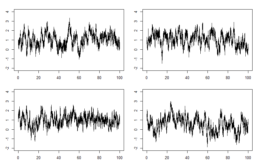
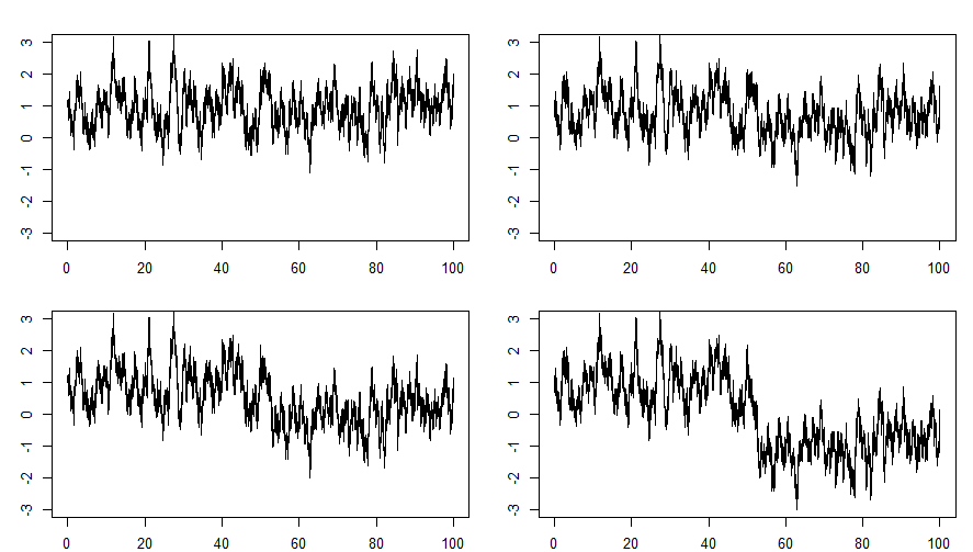
We deal with the testing problem for parameter change in diffusion processes from discrete observations , where and is a positive sequence such that and . We further assume . In order to analyze stochastic phenomena, we construct a statistical model with statistical inference for unknown parameters. In some cases, the values of the parameters of the model may change due to some influence. For example, if we consider a model of the stock price fluctuation, then the parameters of the statistical model may change due to factors such as interest rates, economic conditions, or political trends. It is important to see if the values of the parameters of this model have changed. That is, we want to determine if there are any changes in such paths. As we see from the paths shown in Figure 1, the parameters of this model may have changed. In particular, it would be nice to be able to determine whether there is a change in the paths as shown in Figure 2. However, it seems difficult to determine whether there are changes in these paths. In this paper, we show that our proposed test statistics detect whether these paths have changed and the tests also tell us whether either the diffusion parameter or the drift parameter changes.

Change point problems for diffusion processes has been developed by many researchers. Kutoyants (2004), Lee et al. (2006), Negri and Nishiyama (2012) and Tsukuda (2017) treated the problem of testing for a change of the drift parameter in continuously observed ergodic diffusion processes. On the other hand, De Gregorio and Iacus (2008), Song and Lee (2009), Lee (2011) and Song (2020) studied the problem of testing for a change of the diffusion parameter for discretely observed diffusion processes, see also Iacus and Yoshida (2012) for the estimation problem for the change point of the volatility in a stochastic differential equation. Song and Lee (2009) considered the testing problem for a change of diffusion parameter for the following stochastic differential equation with known drift function under the assumption . Furthermore, Song (2020) considered the test statistic for a change in the diffusion parameter of the stochastic differential equation with under . Negri and Nishiyama (2017) proposed the test statistics for changes of the diffusion parameter or the drift parameter in the stochastic differential equation. In this paper, we construct the two kinds of adaptive test statistics for the diffusion parameter and the drift parameter . Using the proposed test statistics, we can determine whether either the diffusion parameter or the drift parameter changes.
This paper is organized as follows. In Section 2, we state the main results. We propose the adaptive test statistics and show that the test statistics have limiting distribution of the sup of the norm of a Brownian bridge. In Section 3, examples and simulation studies are given. In Section 4, we provide the proofs.
2. Main results
Let , , , where is the transpose. Let be the space of all functions satisfying the following conditions:
- (i)
is continuously differentiable with respect to up to order for all ;
- (ii)
and all its -derivatives up to order are times continuously differentiable with respect to ;
- (iii)
and all derivatives are of polynomial growth in uniformly in , i.e., is of polynomial growth in uniformly in if, for some , we have
We assume the following conditions:
- [A1]
There exists a constant such that for any ,
- [A2]
for all and .
- [A3]
.
- [A4]
and .
- [A5]
The solution of (1.1) is ergodic with its invariant measure such that
2.1. Test for the diffusion parameter
We consider the following testing problem:
Now, we additionally assume the following condition:
- [A6]
Under , there exists an estimator such that
Let
Note that
and has asymptotic normality, let
The test statistic for is as follows:
For , let be a -dimensional standard Brownian bridge.
Suppose that [A1]-[A6] hold. Then under , as ,
2.2. Test for the drift parameter
We make the following assumption:
- [A7]
does not change over .
Then we consider the following testing problem:
Now, we additionally assume the following condition:
- [A8]
Under , there exists an estimator such that
Let
Note that
and has asymptotic normality, let
The test statistic for is as follows:
Suppose that [A1]-[A5], [A7] and [A8] hold. Then under , as ,
is the simple test statistic, but the test may not be consistent, see Section 3 below. In this case, we consider another test statistic. Let
Note that is a consistent estimator of
The test statistic for is as follows:
We additionally assume the following condition:
- [A9]
There exists an integer such that and .
Suppose that [A1]-[A5], [A7], [A8] and [A9] hold. Then under , as ,
We assume the following condition instead of [A9]:
- [A9’]
There exists an integer such that and for .
Suppose that [A1]-[A5], [A7], [A8] and [A9’] hold. Then under , as ,
Since , and , if for some , then there exists an integer such that . Therefore, in [A9] of Theorem 3, we make the assumption of the smoothness of the drift coefficient with respect to up to order when the drift coefficient is general. In particular, if , then [A9] is satisfied. In contrast, Corollary 4 indicates that when the drift coefficient , we set in [A9’] and there is no need to assume in [A9].
2.3. The powers of tests
First, we consider the power of the test for the diffusion parameter , that is, the following testing problem: does not change over , There exists such that
where . Now, we assume the following conditions:
- [B1]
Under , there exist and an estimator such that
Set
- [B2]
under .
Let and denote the upper- point of , that is, .
Assume [A1]-[A4], [B1] and [B2]. Then, under ,
Hence, if [B1] and [B2] are satisfied, then the test is consistent.
In the following, we assume [A7]. We consider the power of the test for the drift parameter , that is, the following testing problem: does not change over , There exists such that
where . Now, we assume the following conditions:
- [B3]
Under , there exist and estimators and such that
- [B3’]
Under , there exist and estimators and such that
Let
- [B4]
under .
- [B5]
under .
Assume [A1]-[A4], [A7], [B3’] and [B4]. Then, under ,
Assume [A1]-[A4], [A7], [A9], [B3] and [B5]. Then, under ,
Assume [A1]-[A4], [A7], [A9’], [B3’] and [B5]. Then, under ,
Theorems 6, 7 and Corollary 8 indicate that the tests and are consistent under some regularity conditions. Theorem 7 and Corollary 8 indicate that the test is consistent when the drift coefficient satisfies [A9] and [A9’], respectively. In particular, for the drift coefficient satisfying [A9], it is necessary to assume in [B3]. When the drift coefficient satisfies [A9’], it is enough to assume in [B3’]. For the maximum likelihood type estimators of the misspecified diffusion processes, see Uchida and Yoshida (2011).
3. Examples and simulation results
In this section, we evaluate the asymptotic performance of the test statistics , and through a simulation study. In this study, we consider the -dimensional Ornstein-Uhlenbeck process (OU process):
| (3.1) |
The data are obtained discretely with sampling interval , so that .
Song and Lee (2009), Lee (2011) and Song (2020) conduct the simulations for the test statistic of the diffusion coefficient. On the other hand, we also perform the simulations for the test statistic of the drift coefficient as well as the diffusion coefficient. In addition, Negri and Nishiyama (2017) perform the simulations for the test statistic of the diffusion and drift parameters at the same time. In our case, however, we first test the diffusion parameter, and if we determine that there is no change in the diffusion parameter, then we test the drift parameter. They are the adaptive tests for the changes of both the drift and the diffusion parameters. As far as we know, this is the first numerical simulations of the adaptive tests for the change point problem of an ergodic diffusion process. For details of the adaptive tests based on the Wald type test statistics and the Rao type ones and the likelihood ratio type ones for ergodic diffusion processes, see Kitagawa and Uchida (2014).
Under the above setting with and for , we have
where is an estimator satisfying the assumption [A6] or [A8], and we construct the estimator from
see, for example, Kessler (1995, 1997), Uchida and Yoshida (2012) and Kaino and Uchida (2018). We have, from Theorems 1, 2 and Corollary 4,
| (3.2) |
In order to evaluate the empirical sizes and powers of and , we consider three cases as follows:
- Case 1:
-
Neither parameter changes.
- Case 2:
-
The diffusion parameter changes.
- Case 3:
-
The diffusion parameter does not change, but the drift parameter changes.
For each of the above cases, we change parameters at . The empirical sizes and powers are calculated as the rejection number of the null hypothesis out of 1,000 repetitions. All simulations are conducted at significance level and the corresponding critical values are obtained from the following: the standard Brownian bridge is generated by taking points on the interval , and the maximum value of its norm is recorded. This is repeated times. As a result, we have
i.e., the corresponding critical values are 1.223 and 1.444 for the 1-dimensional and 2-dimensional standard Brownian bridges, respectively.
In Case 1, we confirm that (3.2) holds with various parameters.
Next, we consider the empirical sizes of ,
and .
The empirical sizes are calculated for the OU process with
,
.
In (i) of Case 2, we confirm that is consistent, that is, the power of goes to under the following situation:
- (i)
the only parameter changes from to .
Lee (2011) also performed this simulation, but we consider the cases where the parameter change is small and the number of data is large.
In Case 3, after confirming that , it is verified whether and are consistent. We consider the empirical size of and the powers of and under the following situations:
- (i)
the parameter only changes from to ;
- (ii)
the parameter only changes from to ;
- (iii)
the parameter changes from to .
and in OU process (3.1) represent the speed of reversion and the mean value as , respectively. In (i) and (ii), we verify the consistency of the test when each parameter changes, and in (iii), we also verify the consistency of the test when both and change.
First, let us consider the consistency of the test based on . The invariant measure of the solution in (3.1) is , , and we have
Therefore, noting that , for , and the test has consistency according to Theorem 5.
Next, we investigate the consistency of the test . For the drift parameter , we have
where .
We construct the estimators and in the same way as above. Since
where
if we set , then under .
Since ,
and
we have
If and , then
and [B4] does not hold. If , then
and the test has consistency according to Theorem 6.
Furthermore, we study the consistency of the test . One has
and
If , noting that , then
If and , then
Therefore, the test is consistent by Corollary 8.
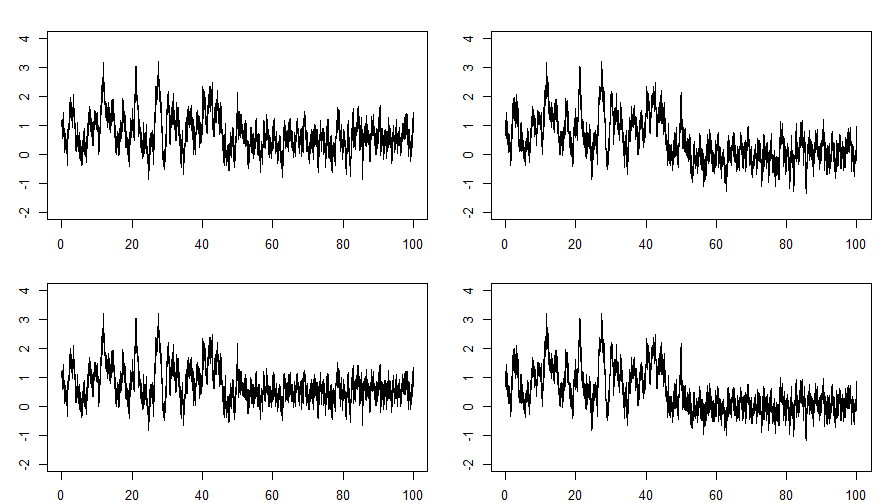
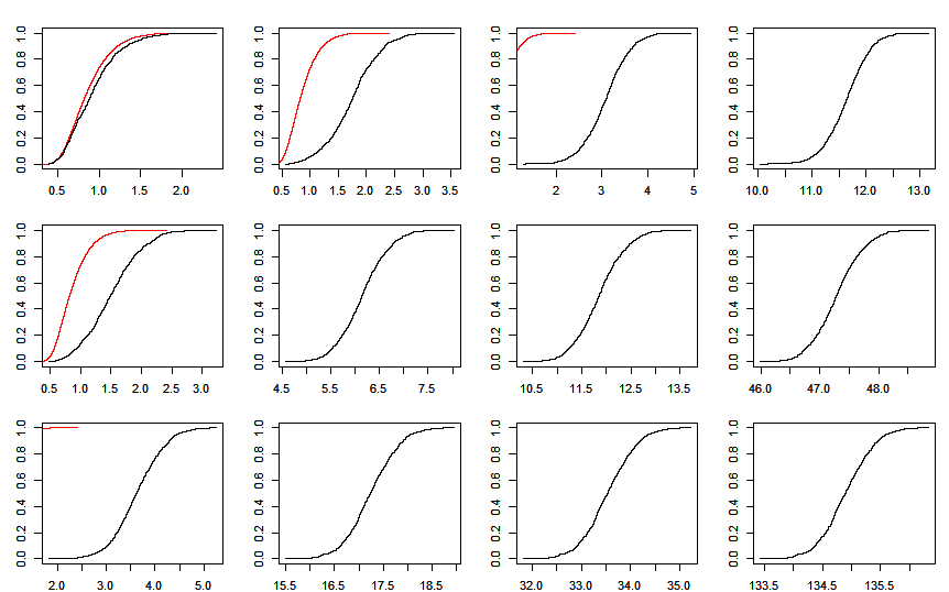
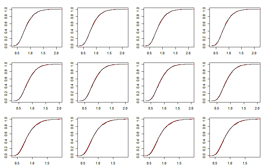
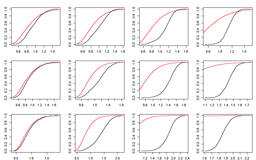
Figures 4-8 show the sample paths in Case 1, (i) of Case 2 and (i)-(iii) of Case 3, and Figures 8-20 show the histograms of and and the probability density function of and obtained by the simulation in the above cases. Figures 22-33 show the empirical distribution function of and and the cumulative distribution function of and .
Table 1 shows the empirical sizes of and in Case 1 when and . According to Table 1, the empirical sizes of and are around 0.1 for each and . Furthermore, from Figures 8-10 and Figures 22-24, we can see (3.2).
Table 2 shows the empirical powers of in Case . According to Table 2, if , the changes as shown in Figure 4 is detected. We can confirm this from Figures 12 and 24.
Tables 3-5 show the empirical sizes of and empirical powers of and in Case 3. First, in (i)-(iii) of Case 3, are about 0.1, and we can confirm from Figures 12, 16, 18, 26, 28 and 32. It can be seen from Table 3 that does not give good results in (i) of Case 3. As seen above, since does not satisfy the sufficient condition [B4] for having consistency in (i) of Case 3, it can be guessed that may not have consistency in (i) of Case 3. In contrast to , gives good results in (i) of Case 3. We can confirm them from Figures 14, 14, 26 and 28. Similarly, when changes in (ii) of Case 3, we can see from Table 4, Figures 16 and 28, and the consistency of and from Figures 16, 18, 30 and 30. Moreover, in (iii) of Case 3, we can confirm from Table 5, Figures 18 and 32 and the consistency of and from Figures 20, 20, 32 and 33.
| 20 | 0.106 | 0.107 | 0.107 | 0.107 | |||
|---|---|---|---|---|---|---|---|
| 0.095 | 0.078 | 0.091 | 0.097 | ||||
| 0.091 | 0.083 | 0.087 | 0.090 | ||||
| 50 | 0.100 | 0.099 | 0.099 | 0.100 | |||
| 0.093 | 0.102 | 0.109 | 0.115 | ||||
| 0.098 | 0.095 | 0.091 | 0.106 | ||||
| 100 | 0.119 | 0.118 | 0.119 | 0.118 | |||
| 0.106 | 0.104 | 0.107 | 0.102 | ||||
| 0.097 | 0.096 | 0.095 | 0.095 | ||||
| 1.01 | 1.05 | 1.1 | 1.5 | |||
|---|---|---|---|---|---|---|
| 20 | 0.144 | 0.864 | 1.000 | 1.000 | ||
| 50 | 0.741 | 1.000 | 1.000 | 1.000 | ||
| 100 | 1.000 | 1.000 | 1.000 | 1.000 | ||
| 1.1 | 1.5 | 3 | 5 | ||||
|---|---|---|---|---|---|---|---|
| 20 | 0.106 | 0.107 | 0.102 | 0.102 | |||
| 0.095 | 0.112 | 0.208 | 0.296 | ||||
| 0.100 | 0.152 | 0.532 | 0.918 | ||||
| 50 | 0.099 | 0.101 | 0.101 | 0.097 | |||
| 0.101 | 0.119 | 0.204 | 0.296 | ||||
| 0.119 | 0.247 | 0.906 | 0.999 | ||||
| 100 | 0.119 | 0.118 | 0.118 | 0.116 | |||
| 0.108 | 0.129 | 0.220 | 0.302 | ||||
| 0.126 | 0.351 | 0.998 | 1.000 | ||||
| 0.9 | 0.5 | 0 | |||||
|---|---|---|---|---|---|---|---|
| 20 | 0.106 | 0.106 | 0.104 | 0.102 | |||
| 0.103 | 0.170 | 0.287 | 0.210 | ||||
| 0.093 | 0.118 | 0.158 | 0.075 | ||||
| 50 | 0.100 | 0.100 | 0.100 | 0.100 | |||
| 0.108 | 0.378 | 0.852 | 0.990 | ||||
| 0.102 | 0.277 | 0.621 | 0.641 | ||||
| 100 | 0.119 | 0.119 | 0.119 | 0.119 | |||
| 0.121 | 0.680 | 0.996 | 1.000 | ||||
| 0.115 | 0.574 | 0.980 | 1.000 | ||||
| 20 | 0.102 | 0.102 | 0.100 | 0.101 | |||
|---|---|---|---|---|---|---|---|
| 0.458 | 0.758 | 0.585 | 0.860 | ||||
| 0.676 | 0.735 | 0.961 | 0.962 | ||||
| 50 | 0.100 | 0.100 | 0.096 | 0.096 | |||
| 0.720 | 0.992 | 0.808 | 0.996 | ||||
| 0.989 | 1.000 | 0.999 | 1.000 | ||||
| 100 | 0.118 | 0.119 | 0.116 | 0.116 | |||
| 0.931 | 1.000 | 0.956 | 1.000 | ||||
| 1.000 | 1.000 | 1.000 | 1.000 | ||||

((i) of Case 2).








4. Proofs
Let , and , denote universal constants. If is a function on , denotes the value . If is a positive sequence, denotes a function on for which there exists a constant such that
Let .
Suppose that [A1]-[A4] hold. Then for ,
| (4.1) | ||||
| (4.2) | ||||
| (4.3) |
Let
Suppose that [A1]-[A4] hold. Then,
| (4.4) | ||||
| (4.5) | ||||
| (4.6) | ||||
| (4.7) | ||||
| (4.8) | ||||
| (4.9) |
Suppose that [A1], [A2], [A5] hold and a function on satisfies
- (i)
is continuous in for all ;
- (ii)
exists and are of polynomial growth in uniformly .
Moreover, if for some , then, under (or [A7] and ), as ,
Suppose that [A1], [A2], [A5] hold and satisfies the conditions (i), (ii) in Lemma 3. Then, under (or [A7] and ), as ,
Proof.
Suppose that [A1]-[A5] hold and satisfies the conditions (i), (ii) in Lemma 3. Then, under (or [A7] and ), as ,
| (4.10) | ||||
| (4.11) |
Proof.
Proof of Theorem 1.
Let
By Taylor expansion, we have
where
Then, we can express
Therefore, it is enough to show
| (4.14) | ||||
| (4.15) | ||||
| (4.16) |
Proof of (4.14). Let be a -dimensional standard Brownian motion. in denotes that weakly converges to in the Skorohod space on . If we prove
| (4.17) |
then, it follows from the continuous mapping theorem that
According to Corollary 3.8 of McLeish (1974), we obtain (4.18) if we prove
| (4.20) | ||||
| (4.21) | ||||
| (4.22) |
for all .
(4.20) is obvious. From Lemma 1, we have
and
Hence (4.21) holds. Since ,
Therefore we obtain (4.22). This completes the proof of (4.14).
Proof of (4.16). Since , there exists an open neighborhood of such that . If , then
and
Hence, from [A6], we have and, for all ,
Therefore we obtain
and
∎
Proof of Theorem 2.
Let
By the Taylor expansion, we have
where
Then, we can express
Therefore, it is enough to show
| (4.23) | ||||
| (4.24) | ||||
| (4.25) | ||||
| (4.26) | ||||
| (4.27) | ||||
| (4.28) |
It follows from Corollary 3.8 of McLeish (1974) that one has (4.30) if we prove
| (4.32) | ||||
| (4.33) | ||||
| (4.34) |
for all .
Proof of Theorem 3.
Let
By the Taylor expansion, we have
where
Then, we can express
We set
Note that, by the Taylor expansion,
where
Then,
and
Moreover,
Note that and
Therefore, it is enough to show
| (4.35) | ||||
| (4.36) | ||||
| (4.37) | ||||
| (4.38) | ||||
| (4.39) | ||||
| (4.40) | ||||
| (4.41) | ||||
| (4.42) | ||||
| (4.43) |
According to the Cramér-Wold theorem and Corollary 3.8 of McLeish (1974), we obtain (4.45) if we show that for all ,
i.e.,
| (4.47) | ||||
| (4.48) | ||||
| (4.49) |
for all .
(4.47) is obvious. From Lemma 1,
i.e., (4.48) holds. Since ,
Therefore we obtain (4.49). This completes the proof of (4.35).
Proof of Corollary 4.
Proof of Theorem 5.
If we prove
| (4.50) | ||||
| (4.51) |
then, we see from [B2] that
and
i.e.,
Therefore, we have .
Let us show (4.50). We can express
From Lemma 1, we have
and
Therefore, from Lemma 9 of Genon-Catalot and Jacod (1993),
| (4.52) |
On the other hand, from [B1] and
we have
| (4.53) |
Hence, it follows from (4.52) and (4.53) that we obtain (4.50). In the same way, noting that if , we have (4.51), which completes the proof of Theorem 5. ∎
Proof of Theorem 6.
If we prove
| (4.54) | ||||
| (4.55) |
then, it follows from [B4] that
and
i.e.,
Hence, one has .
Let us show (4.54). We can express
From Lemma 1, we have
and
Therefore, from Lemma 9 of Genon-Catalot and Jacod (1993),
| (4.56) |
On the other hand, from [B3’] and
we have
| (4.57) |
and
| (4.58) |
Hence, from (4.56), (4.57) and (4.58), we obtain (4.54). In the same manner, noting that if , we have (4.55), which completes the proof of Theorem 6. ∎
Proof of Theorem 7.
If we prove
| (4.59) | ||||
| (4.60) |
we obtain, from [B5],
and
i.e.,
Proof of Corollary 8.
References
- [1] [] Billingsley, P. (1999). Convergence of probability measures. Second edition. Willy, New York.
- [2] [] De Gregorio, A., Iacus, S. M. (2008). Least squares volatility change point estimation for partially observed diffusion processes. Communications in Statistics - Theory and Methods, 37, 2342-2357.
- [3] [] Genon-Catalot, V., Jacod, J. (1993). On the estimation of the diffusion coefficient for multidimensional diffusion processes. Annales de l’Institut Henri Poincaré Probabilités et Statistiques, 29, 119-151.
- [4] [] Hall, P., Heyde, C. C. (1980). Martingale limit theory and its application. Academic Press, New York.
- [5] [] Iacus, S. M., Yoshida, N. (2012). Estimation for the change point of volatility in a stochastic differential equation. Stochastic Processes and their Applications, 122, 1068-1092.
- [6] [] Kaino, Y., Uchida, M. (2018). Hybrid estimators for stochastic differential equations from reduced data. Statistical Inference for Stochastic Processes, 21, 435-454.
- [7] [] Kessler, M. (1995). Estimation des paramètres d’une diffusion par des contrastes corrigés. Comptes rendus de l’Académie des sciences. Paris Serie I 320, 359-362.
- [8] [] Kessler, M. (1997). Estimation of an Ergodic Diffusion from Discrete Observations. Scandinavian Journal of Statistics, 24, 211-229.
- [9] [] Kitagawa, H., Uchida, M. (2014). Adaptive test statistics for ergodic diffusion processes sampled at discrete times. Journal of Statistical Planning and Inference, 150, 84-110.
- [10] [] Kutoyants, Y. A. (2004). Statistical inference for ergodic diffusion processes, Springer.
- [11] [] Lee, S. (2011). Change point test for dispersion parameter based on discretely observed sample from SDE models. Bulletin of the Korean Mathematical Society, 48, 839-845.
- [12] [] Lee, S., Nishiyama, Y., Yoshida, N. (2006). Test for parameter change in diffusion processes by cusum statistics based on one-step estimators. Annals of the Institute of Statistical Mathematics, 58, 211-222.
- [13] [] McLeish, D., L. (1974). Dependent central limit theorems and invariance principles. The Annals of Probability, 2, 620-628.
- [14] [] Negri, I., Nishiyama, Y. (2012). Asymptotically distribution free test for parameter change in a diffusion process model. Annals of the Institute of Statistical Mathematics, 64, 911-918.
- [15] [] Negri, I., Nishiyama, Y. (2017). Z-process method for change point problems with applications to discretely observed diffusion processes. Statistical Methods and Applications, 26, 231-250.
- [16] [] Song, J. (2020). Robust test for dispersion parameter change in discretely observed diffusion processes. Computational Statistics and Data Analysis, 142, 106832.
- [17] [] Song, J., Lee, S. (2009). Test for parameter change in discretely observed diffusion processes. Statistical Inference for Stochastic Processes, 12, 165-183.
- [18] [] Tsukuda, K. (2017). A change detection procedure for an ergodic diffusion process. Annals of the Institute of Statistical Mathematics, 69, 833-864.
- [19] [] Uchida, M. and Yoshida, N. (2011). Estimation for misspecified ergodic diffusion processes from discrete observations. European Series in Applied and Industrial Mathematics: Probability and Statistics, Volume 15, 270-290.
- [20] [] Uchida, M., Yoshida, N. (2012). Adaptive estimation of an ergodic diffusion process based on sampled data. Stochastic Processes and their Applications, 122, 2885-2924.