[orcid=0000-0002-0599-7036]
[orcid=0000-0002-3057-6786]
[orcid=0000-0002-8995-7356]
[orcid=0000-0001-5998-3986]
Effects of Dark Energy anisotropic stress on the matter power spectrum
Abstract
We study the effects of dark energy (DE) anisotropic stress on features of the matter power spectrum (PS). We employ the Parametrized Post-Friedmannian (PPF) formalism to emulate an effective DE, and model its anisotropic stress properties through a two-parameter equation that governs its overall amplitude () and transition scale (). For the background cosmology, we consider different equations of state to model DE including a constant parameter, and models that provide thawing (CPL) and freezing (nCPL) behaviors. We first constrain these parameters by using the Pantheon, BAO, and CMB Planck data. Then, we analyze the role played by these parameters in the linear PS. In order for the anisotropic stress not to provoke deviations larger than and with respect to the CDM PS at , the parameters have to be in the range , and , , respectively. Additionally, we compute the leading nonlinear corrections to the PS using standard perturbation theory in real and redshift space, showing that the differences with respect to the CDM are enhanced, especially for the quadrupole and hexadecapole RSD multipoles.
keywords
Large Scale Structure ,Anisotropic Stress ,Dark Energy1 Introduction
The discovery of the accelerated expansion of the Universe implied the existence of dark energy (DE), that has been extensively confirmed by a two-decade variety of experiments, initially employing Supernovae type Ia [1, 2], then using anisotropies in the CMB from WMAP and Planck data [3], distance measurements of different tracers [4], and clustering of large galaxy surveys, among other probes [5, 6, 7]. However, little is known of the fundamental properties of DE, apart from being a ‘fluid’ that possess negative pressure. In the most successful model a cosmological constant, , is capable to fit the observations, albeit current tensions exist among a few parameters when measured with different probes [8].
The effects of DE have been widely studied in the context of background cosmological dynamics; most of the work has been devoted to test different equations of state (EoS) for DE to understand the dynamics of the Hubble expansion flow. However, in comparison its perturbative effects are less explored, partially because we expect little deviations at perturbative level, but also because we have no clues on its fundamental origin. One can, for example, treat DE as a barotropic fluid, hence, its sound speed depends only on background quantities, or to consider it as a non-adiabatic fluid to account for its linear effects for which additional hypotheses have to be made about the fluid’s speed of sound [9]. There are many works that study the effect of DE speed of sound in the perturbative dynamics, initially done by [10, 11, 12, 13]. It turns out that the effects of DE clustering result to be small, especially if the DE EoS is close to , as demanded by observations, and then they are difficult to discern with late-Universe measurements [14, 15]. But, in fact, varying the DE sound speed can induce deviations of up 2 in the matter power spectrum (PS) [16, 17], that should be important in view of the expected constraints from upcoming galaxy surveys, such as DESI [18].
Another possibility is to consider DE anisotropic stress. A homogenous and isotropic symmetric background metric forbids it, but it can be introduced at the perturbed level [19]. Anisotropic stress can also mimic modified gravity (MG) at linear order [20, 21, 22, 23], since it introduces at least a new parameter, and together with DE EoS and sound speed, it yields a modified growth of structures in the Universe. In fact, DE stress generates similar outcomes as those of varying the sound speed of DE, but the detailed behavior depends on the signs of the EoS and stress parameter [24]. From theoretical grounds, one expects DE anisotropic stress to affect the evolution of the metric potentials and this provokes CMB temperature anisotropies at low-multipoles, to be affected through the Integrated Sachs-Wolfe (ISW) effect. In Refs. [25, 24, 26, 27, 28, 29] DE anisotropic stress was analyzed to prove this conclusion using CMB data available at that time, but due to the cosmic variance, CMB constraints are still broad. However, DE stress should affect also matter clustering at large scales. Effects of anisotropic stress on the matter power spectrum (PS) and on the growth function have been studied in several works [25, 24, 30, 31, 32, 33, 34], showing that shear viscosity has an effect on very large scales, but one the other hand it does not change much other cosmological parameter values; for instance, for this latter reason we do not expect that DE shear terms alone can alleviate the current tension in the Hubble constant; see however [35] in which it is proven that adding anisotropic shear to interacting models helps to increase the Hubble constant to release the tension for phantom DE.
In the literature there is a number of works considering different aspects of imperfect fluids, e.g. in connection to second order perturbation in CDM [36], or related to generalized scalar fields [37, 38]. Also, based on MG, efforts have been put forward to understand how the gravitational effects of the fifth-force (that generates an effective shear term) influence the observables at cosmological scales, changing the clustering properties [39, 40]. Our motivation here, linked to these latter works, is to analyze the anisotropic stress effects on CMB and matter PS since the level of accuracy of future LSS galaxy surveys and probes shall demand detailed understanding of the clustering properties of the matter field. In this way, being able to constrain an hypothetical anisotropic shear, stemming either from DE or MG. Ways to carry out this comparison are discussed e.g. in Refs. [41, 42, 43]. Recently, analysis of recent probes hints for non-zero anisotropic stress [44], that also encourages us to further analyze its clustering properties.
In the present work, we use the Parametrized Post-Friedmannian (PPF) approach [45, 26, 46], though originally motivated to emulate MG models, they naturally introduce an effective DE anisotropic stress term. In this respect, the formalism serves to phenomenologically introduce either DE stress or effective MG stress terms. Viewed as effective DE, we consider specific equations of state and fix the DE speed of sound, to concentrate our analysis on the effects of the anisotropic stress. We analyze the constraints from CMB power spectra and, especially, look for deviations in the PS. Interestingly, we find that DE anisotropic stress is allowed by Planck CMB data, as in Refs. [24, 26], but the linear and nonlinear PS impose tighter constraints to it. We consider different DE EoS, firstly that emulates at background level, then constant , and finally, thawing and freezing models, to find out their effects in combination with stress parameters.
The structure of this paper is the following: In Section 2 we motivate DE EoS parametrizations chosen, and in Section 3 we introduce the DE perturbation theory with anisotropic stress, where a specific anisotropic stress phenomenology is adopted. Section 4 shows our results employing different EoS, and Section 5 shows the theory and results for nonlinear perturbation theory to 1-loop. Finally, Section 6 concludes.
2 Dark energy Equation of State
Beyond a cosmological constant, the accelerated expansion of the Universe can be driven by a dynamical DE component whose EoS is commonly parametrized by a time dependent function
| (1) |
where the EoS parameter, , can be chosen with different purposes; as for example, it can mimic quintessence and phantom fields [47, 48]. In general, EoS parameterizations can be classified into two broad categories: thawing and freezing behaviors [49, 50]. In the first case the scalar field is frozen at early times where the kinetic energy is negligible and , then evolves generically as a monotonic, convex, decreasing function to reach asymptotically, at late times, some . In the second case, in freezing-tracker models, the scalar field rolls down to the minimum of its potential at the beginning of the Universe, but starts to slow down and stops when it comes to dominate the dynamics; in this case the function is generically a monotonic, concave, increasing function at higher which at late times tends to . Several DE parametrizations have been proposed in the literature, some seem to favor thawing models [51, 52], but Ref. [53] exhibits that freezing models fit better. This latter reference proposes a generalization of the CPL EoS [54, 55], called nCPL,
| (2) |
such that reduces to the standard CPL (suitable for thawing models) while for larger values of it can produce freezing behavior. Since our goal is to understand how different EoS behaviors influence CMB anisotropies and the PS, especially in combination with anisotropic stress, we will consider the nCPL parametrization with and , corresponding to thawing and freezing behaviors, respectively. We will also consider models with constant. For any , the nCPL EoS parametrization is at and goes to at high redshifts. A requirement to achieve a thawing behavior is that the function should be decreasing as grows and so must be negative, and to get a freezing evolution must be positive.
The energy density for nCPL evolves as
| (3) |
which together with the other matter components it determines the background history, , through the Friedmann equation.
3 Dark energy fluctuations
We consider a perturbed metric around a Friedmann-Lemaitre-Robertson-Walker (FLRW) spacetime in Newtonian, longitudinal gauge,
| (4) |
where and are the gauge invariant scalar potentials [56, 57]. The components of the energy momentum tensor are
| (5) |
where and are the energy density and pressure at the background, and their pertubations, and are the anisotropic stress components. Since we are dealing with scalar perturbations, it is useful to work with the velocity divergence and the scalar anisotropic stress defined as
| (6) | ||||
| (7) |
From Einstein’s field equations one obtains
| (8) | ||||
| (9) |
where the sums run over all energy components. In the absence of anisotropic stresses both gravitational potentials are equal (up to a minus sign). At early times the difference in the two gravitational potentials is sourced by the second moment of the phase-space distribution function of radiation components. However at late times, well after decoupling and during the matter dominated phase, this is negligible and one can safely set to obtain the standard growth of matter linear perturbations . This is a key property of cold dark matter (CDM), allowing its perturbations to grow at the same rate for all scales well below the Hubble horizon during the matter dominated phase. At later times, once DE starts to become important, the growth of large scales structures is halted because the expansion becomes very fast and the pace of matter aggregation is reduced, even frozen for a de Sitter expansion. The details of how this process occurs depend on the very nature of DE. Matter components source the gravitational potential through the Poisson equation, Eq. (8), however the trajectories of non-relativistic CDM particles respond to the gravitational potential through the geodesic equation, which in the Newtonian limit is . Hence, even if probes of the Universe’s expansion indicate that DE should very close to a cosmological constant with , the growth of perturbations can be very different in the presence of the anisotropic stress . But note that this quantity is not accessible from background observations, and by taking a posture of complete ignorance about what DE is, it is natural to incorporate the stress in a perturbative analysis, on the same footing as one introduces the EoS and the speed of sound. The anisotropic stress should be small at early times, before decoupling, in order to not spoil the CMB anisotropies, tightly constraining models and leaving room to affect the CMB only through the ISW effect. Hence, it is expected that effects of a DE stress will be more feasible to be detected through CDM late time clustering probes, in particular the matter PS.
From the conservation of the energy-momentum tensor we get the continuity and Euler equations, for non-interacting fluids these reduce to
| (10) |
| (11) |
where we use derivatives with respect to , denoted by a prime. At the background level adiabaticity is guaranteed by the continuity equation, however, when fluctuations are considered, the energy density of components and their EoS do not completely specify their pressure. In a general description, for non-interacting components one has the relation [58, 59, 13]
| (12) |
with the adiabatic sound speed and the speed of sound in the fluid’s rest frame,
| (13) |
where
| (14) |
is the gauge invariant rest-frame density perturbation [56].
3.1 Dark energy anisotropic stress
There are different approaches to implement the evolution of DE anisotropic stress to solve the system (8)-(11). Some works [24, 25, 28, 29, 32, 34, 60] assume that anisotropic stress is sourced by the amplitude of the velocity shear tensor , and are motivated by the fact that it should be gauge invariant; so they demand to fulfill a continuity-like equation stemming from a Boltzmann hierarchy, but invoking an effective viscosity parameter as a source. This approach washes out DE fluctuations for non-phantom EoS [30], making them even more difficult to detect when compared to other approaches, as those motivated by MG [33] or modified growth [21], where effects inside the horizon are also expected. Both approaches are valid and are motivated by different physics. The specific model will then determine the effects on observables. Our motivation is to explore effects on scales that will be available through the next generation of LSS measurements.
In this work, we will use the PPF prescription presented in Refs. [45, 26, 46], originally motivated to parametrize MG models that naturally introduce an effective anisotropic stress term. In this view, DE is a phenomenon of a geometric theory. This approach studies perturbation modes larger and smaller than the horizon and, therefore, it needs to impose two conditions on the field equations in order to preserve covariant conservation laws for the fluids. The first condition requires that the curvature in the comoving gauge is only changed by the effective DE at second order in . The second condition is that the metric potential satisfies a Poisson-like equation in the quasi-static limit. Following this formalism, one introduces the effective DE shear in Eq. (9) through
| (15) |
where , and the subindex is for the sum of total matter components, that in our case excludes DE. Equation (15) defines the function , which relates the two metric potentials and encodes the information of effective DE anisotropic stress as
| (16) |
thus, instead of using , one can work with . In the absence of stresses other than DE, as it happens at late times, is related to the more commonly used slip parameter as
| (17) |
reducing to DE stress-free models when . Below we will choose specific parametrizations for that are negligible at early times, when the stresses from radiation components are important. Hence, the stresses due to DE and other components are essentially not coupled, and we can think of this PPF formalism as a DE parametrization, instead of MG.
Using Eqs. (8) and (9) we obtain the constraint
| (18) |
which reduces to the Poisson equation, Eq. (8), in the absence of anisotropic stresses.
The PPF formalism further introduces a couple of functions to encompass physical conditions in the limits of modes much larger and much smaller than the Hubble horizon. At large scales, one has that
| (19) |
so that effective DE is parametrized by at large scales.
In the opposite limit, for modes well inside the horizon, DE is smooth compared with matter and the metric potential satisfies
| (20) |
which has the form of a Poisson equation for the potential with Newton’s constant rescaled by and it is sourced by anisotropic stresses of other components, different from DE, that can be safely neglected at late times.
In addition, one introduces the function , which encodes the DE contributions and allows to express the source of an effective potential in terms of matter variables only as
| (21) |
A comparison between Eqs. (18) and (21) relates function with DE quantities
| (22) |
should fulfill the two above mentioned limits, hence the PPF formalism constructs the equation of motion [45, 26]
| (23) |
where is a constant that modulates the transition scale between the two limits, and
| (24) |
such that Eq. (23) satisfies both limits
| (25) |
These are all the required equations and conditions for the DE PPF prescription. Once functions , and are given, it is possible to solve for to finally recover the effective DE quantities.
In terms of these functions the rest frame DE density perturbation is
| (26) |
and can be obtained through
| (27) |
The potential is associated to the ISW effect, and we will obtain that for a positive, increasing function of time , it will cause an increase of the low- CMB anisotropies.
The DE anisotropic stress contribution can be written as:
| (28) |
By construction, in the PPF formalism, DE anisotropic stress receives contributions of all energy density perturbations and the different components are multiplied by the same factor. In contrast, other approaches [33, 61] consider different weights to the source terms of Eq. (28) aiming at suppressing shear terms at large scales.
3.2 Dark energy stress phenomenology
To solve the equations in the PPF formalism, the functions , and , and the constants and should be specified. We know that DE becomes important and not negligible at large scales, this is the limit , where we can expect and at least , also we expect . Motivated by MG models,
we set , though its exact choice is rarely important for observable quantities, see [45, 26]. Varying the DE sound speed () it is known to provoke variations of up 2 in the matter power spectrum [16], but we fix it a constant here, , to concentrate our analysis on the anisotropic stress. And we further assume , inspired to match the evolution of scalar fields, following Ref. [46]. In the opposite limit, , we want to have an effective DE that emulates CDM, thus we will fix .
It is necessary to specify the anisotropic stress function , and its election must obtain deviations when and where it is desired to test them. As explained, large modes affect the ISW signal, and we want to evaluate how much the cosmic variance allows deviations from CDM to later analyze the effect in the matter PS. Also, we would like to observe effects at different scales. In this work we use the function proposed in [26],
| (29) |
which becomes -independent for and goes quickly to zero at small scales. The constant is a transition parameter that determines the modes that plays a role with respect to the Hubble horizon. On the other hand, DE should start to be important at late times when it becomes to dominate over the other matter components, so it seems natural to think of a dependency on the ratio among densities which grows with , motivating the time dependence form of as
| (30) |
Hence, the function introduces two free parameters, its amplitude and the transition scale along -modes. Different combinations of the two anisotropic stress parameters can achieve similar effects in the effective anisotropic shear; however, when we compare to observations (see below) we find no degeneracies between these two parameters. As the scale factor tends to zero, so it does and it does not spoil CMB acoustic oscillations prior to last scattering. It will, on the other hand, have effects on the ISW and the clustering properties of matter fields. For one recovers the case without anisotropic stress, implies scale free dependence, and for high the stress goes to zero, so it has no impact over small structures.
4 Effects of DE anisotropic stress on power spectra
We adapted the codes CAMB11
1
https://camb.info/ [62] and CosmoMC22
2
https://cosmologist.info/cosmomc/. [63] to include the shear contribution as detailed in the previous sections.
We analyze the outcomes of the above anisotropic stress phenomenological model in combination with the effects of different DE EoS. The cosmological data set used in this work is: BAO measurements from
6dFGS, SDSS-MGS, and BOSS LOWZ BAO [64, 65, 66, 67], supernovae from the combined Pantheon
Sample [68], recent measurement from Riess 2018 [69], high- CMB TT spectrum and low- polarization data from Planck 2015 [3]. The main results are separated considering different DE EoS parametrizations that are detailed in the upcoming subsections.
4.1
DE emulating a cosmological constant at background level has no density perturbations in the absence of DE anisotropic stress. However, one expects that evolving DE will have differences, albeit small, from . But, for all practical purposes many DE/MG models are indistinguishable from CDM at background level, so for definiteness we adopt in this subsection. The inclusion of anisotropic stress generates fluctuations that depend on the chosen anisotropic stress parameters: bigger values generate bigger perturbation amplitudes; and, bigger values shift the anisotropic shear effects to larger scales. These behaviors are shown in Fig. 1, where ratios of DE to matter rest-frame densities are plotted for parameters and . These values are chosen because they lie inside the 1- and 2- confidence interval levels (c.l.) allowed by the Monte Carlo Makov Chain (MCMC) (as we will show in Fig. 6), and still provide large deviations to the matter PS, reaching a maximum of 15% when compared to the CDM () case, as explained below.

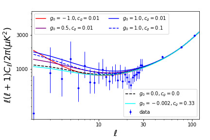
We varied the parameters (, ) using CAMB to obtain various CMB TT power spectra, as shown in Fig. 2, along with CMB Planck data [3]. For fixed, positive values enhance low- anisotropies due to the ISW, whereas negative values diminish them, except for very low multipoles, where multipoles can go crossing the CDM curve to overtake it.
We also show the CDM best fit (black dashed line), labeled in the figure as .
We note that setting fixed, the effect of increasing is both to decrease the low- anisotropies and to shift their effect to smaller -modes. This plot exhibits that, as we expected, the anisotropic parameters are not affecting high -multipoles, where all the plotted curves coincide. For low-multipoles anisotropies, one may try to adjust downwards the curve, however, the relevance of these data points lies in the cosmic variance. In fact, low multipoles, including the quadrupole, turn out to be consistent with the CDM model [70].
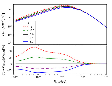
Large scale anisotropic stress imprints an effect on the clustering of matter at late times, as in the PS and growth function [24, 25, 30, 31, 32, 33, 34]. To see this, we plot the PS in Fig. 3 for (, ) parameter values such that is fixed and takes values between , in a similar way we did it in Fig. 2. The effects over this matter statistic are clear: negative values of tend to rise the PS for low -modes, and for large we recover the CDM model since ; positive values produce the opposite effect. Note that we have fixed the normalization such that all models have the same primordial power spectrum amplitude and spectral index . For that reason all models coincide for modes , where becomes negligible.
Now, selecting some of the parameters of Fig. 2, we show in Fig. 4 again the percentage departures with respect to the CDM model: increases the effect. These deviations in the PS amplitude can be large in the range of linear perturbations, and in fact they will also contribute to the nonlinear PS, that we shall study in Section 5.
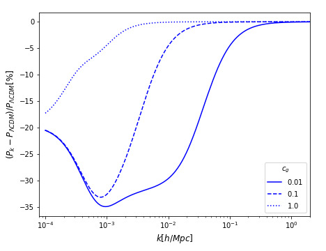
We know, however, that deviations from the CDM PS at scales - could not be as large as in Fig. 3 or 4, since these would affect the BAO features, and given the upcoming galaxy surveys such as DESI [18], the constraints will tighten to uncertainties to be less than (or order of) . Consequently, we explore for deviations that are of the order of and at most (up to an overall normalization) in Fig. 5, left and right panels, respectively. Note that the deviations from CDM reach their maximum around . At the scale , deviations are of 10% (left panel, models , ) and of 0.66% (right panel, models ) and at of 4% (left panel) and of 0.3% (right panel).
In both panels of Fig. 5, dashed lines are for , solid lines for and color changes for different as it is shown in the labels. Negative values of will increase the potentials wells, as can be seen from Eq. (27), and then the PS increases as well. Increasing lowers the absolute value of the maxima () or minina (), but this is a by-effect of the produced shift along , that erases shear fluctuations above . Here we appreciate that deviations of at most 15% are possible if . In the right panel, we find values in the interval permit at most order deviations from the CDM model.


To find out what anisotropic parameter values are more realistic and preferred by cosmological data we perform an MCMC sampling of the parameter space using CosmoMC and the cosmological data set described at the beginning of this section.
The relevant best-fit values for the model without and with DE anisotropic stress are in columns I and II, respectively, of Table 1. For anisotropic parameters we obtain at c.l., in agreement with the results of the vanilla CDM cosmological parameters from Planck [3].
The CMB TT power spectrum produced by these values is included in Fig. 2 (cyan color) that is alike the CDM model, meanwhile other models vary only at low-multipoles, as already explained. Similarly, in the right panel of Fig. 5, we include the PS of our best-fit to obtain deviations of around 0.05% at Mpc from the no anisotropic stress case.
On the other hand, it is common that a comparison of models can be done using the Akaike information criterion (AIC) [71] or the Bayesian information criterion (BIC) [72], such that the model with the minimum AIC/BIC value is considered the best fit model. We compute the differences with respect to CDM, and the results are displayed in table 1. For the model the is considerable less supported than CDM, and similarly shows that the CDM model is stronger supported [73, 74]. The other models in this work also show similar statistics. However, models with DE anisotropic stress possess more degrees of freedom and hence these statistics are a measure of how the added complexity turns into a less favored model. Our intention, though, was not to propose a more simple alternative to CDM, but in fact to add anisotropic stress as a real possibility to the DE nature.
We finalize this subsection presenting the contour confidence region of the stress parameters in Fig.6, confirming that the no-anisotropic case () is allowed at 1- by CMB data. Nevertheless, the left panel of Fig. 5 shows that for anisotropic parameter values that are inside the 2- best-fit values, they produce differences on the PS of at least 15% with respect to CDM. In this parameter range the CMB will be well fitted and not changing significantly. It is then clear that the PS imposes tighter constraints than the CMB on the anisotropic stress and hence is a potential theory discriminator of different DE anisotropic stress models.

| I | II | III | IV | V | VI | |
| CDM | constant | CPL | 7 CPL no-stress | 7 CPL | ||
| 0 | ||||||
| AIC | ||||||
| BIC |
4.2 w = constant
In this section the expansion history is slightly different from CDM, now we assume constant. Thus, density fluctuations are generated even if DE does not possess anisotropic stress, showing that perturbations attenuate as and when .
For this model, anisotropic stress parameters leave very similar imprints on the CMB TT curve as those of the model, see Fig. 2, so we omit to show these results, and the same discussion about the parameters () prevails for this EoS. The effects on the PS are shown in Fig.7, where the EoS reference value is in agreement with Planck’s results [3] and the values and were chosen so that they result in visible changes, with deviations from CDM of order of or less.

For these plots we obtain a maximum deviation of around 10% at , and of at . All anisotropic stress values we used to generate Fig. 7 are consistent with the Planck CMB TT measurements.
The relevant results of an MCMC fit are presented in column II of Table 1, and the contour plots that involve DE parameters are shown in Figs. 6 and 8. The resulting parameters and are similar to the ones produced by the EoS. As expected, the values are inside the 68% contours, meaning that the results are in agreement with the CDM model.
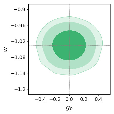

Finally, we note that the values of , reported in Table 1 are similar to the other models. This motivated us to show in Fig. 8 the contour plots of the anisotropic parameters with the EoS parameter to clarify any degeneracy among them. We found essentially no degeneracy in and , and a small effect in and , as also proved in their corresponding correlation matrices in a principal component analysis.
4.3 Thawing parametrization (CPL)
Now we consider the CPL EoS, providing a thawing behavior for . CPL is one of the most popular EoS for DE, and according to Planck 2015 results [3] in the absence of DE anisotropic stress, the best fit values for the data set we are using are , at 2- [75], that we will take as reference values.
We found similar effects due to the anisotropic parameters on the CMB TT power spectrum for this EoS. We plot in Fig. 9 our results on deviations of the PS with respect to CDM model, as in Fig. 5 (left panel) and Fig.7, yielding maximum differences of around ; particularly, at the maximum deviation is about 4%.

Finally, we performed an MCMC statistical analysis parametrizing as CPL. The best-fit parameters and c.l. at 68% are presented in column III of Table 1, and their corresponding contour plots for in Fig. 10. The contour plot for anisotropic stress parameters looks very similar to the one obtained with the EoS ; see Fig. 6, which indicates that the DE EoS and stress parameters are quite independent.

4.4 Freezing parametrization (7-CPL)
Finally we consider the n-CPL DE parametrization, Eq. (2) with which has a freezing behavior if and . To our knowledge, for this EoS there are no reported best-fitted values for . Then, we first estimate them for the case of null anisotropic stress. The results are shown in column IV of Table 1 and the contour plot is presented in Fig.11 (yellow regions).

For this EoS the standard cosmological model is recovered (, ) at 68%. The parameter is well restricted by late time observations, whereas is not sensitive to these cosmological data set, its upper limit at 68% is 0.882 but it can take a wide range of negative values. This is consistent with claims in the sense that fittings suggest thawing [51, 52] and freezing models [53]; we find that both are allowed for this EoS. Variations on are not visible in the CMB TT, but deviations are present in the amplitude of the matter PS. When varying from to the change in the PS is of about 1 in linear scales and these tend to lower the power, the larger (positive) values are. In this case, the effects in the PS occur in between and Mpc; after /Mpc the PS behaves as CDM.
Now we introduce DE anisotropic stress as in the above subsections. The data fits are shown in column V of Table 1, and their contour plots concerning to DE stress parameters are in Fig. 10. The contour plot is shown in Fig. 11 (purple regions) together with that of no-anisotropic stress. The similarity between both cases shows that data from CMB and late time background evolution are agnostic to the presence of the DE anisotropic stress.
In Fig.12 we include the best-fitted values of this model and others inside the 95% contour confidence plot to obtain deviations on the PS of around with respect CDM.

The lesson from all these models is that they leave particular and potentially detectable features in the PS, even when the parameter space for DE EoS and anisotropic parameters are allowed by CMB and background probes. In general, we found that the anisotropic stress provokes deviations smaller than with respect to the CDM PS at for the parameters in the range , and smaller than for , .
5 Nonlinear evolution
Our treatment until here has been limited to linear physics. In the present section we now explore the PS behavior produced by the nonlinear evolution at quasi-linear scales. That is, we will consider some selected values of the above parameters and evolve the system with the standard tools of nonlinear perturbation theory. We will consider the real space PS obtained using standard perturbation theory and the redshift-space multipoles using the TNS model [76]. Hence, the objective of this section is to show how the features produced by the dark energy anisotropic stress in the linear power spectrum evolve when one considers the quasi-linear regime both in real and redshift space. Since such features are located in linear and mildly non-linear regions of the power spectrum, they are amenable for a standard study within perturbation theory, and it is natural to expect that they become enhanced when compared to the linear results. We remark that the results of this section are not used to compare to observations; that would be erroneous, because one would has to tailor a halofit model for these specific models, which is beyond the scope of this work.
The most common approach adopted to study MG/DE models beyond the linear regime is by parametrizing the Poisson equation [77] with a function , which quantifies the deviation of the gravitational Newton constant from the expected value in GR without DE perturbations; in DE models with anisotropic stress, this should be understood as due to the differences in the gravitational potentials and , and not as a modification to GR, as discussed in Section 3.1. The Poisson equation reads
| (31) |
with the matter density contrast. Since nonlinearities are developed at late time we can neglect the contributions of radiation components, and keep only those of matter (combined CDM + baryons) and DE. We identify
| (32) |
In our case, we can construct the function with the linear theory developed in the previous sections and with the ingredients obtained from CAMB. Notice that in writing Eq. (31) we can approximate the matter gauge-invariant overdensity as , since matter particles are non-relativistic and we are interested on scales well inside the Hubble length . With Eqs. (31) and (32) we can construct a Standard Perturbation Theory (SPT) following the recipes developed in Ref. [78, 79, 80] for MG models, that can be adapted to DE models with stress. The formalism consists
first in constructing the kernels that appear in the higher than linear order overdensities, such that at order in SPT one has
| (33) |
where is the linear matter overdensity treated in the previous sections. Thereafter, we can construct the corrections to the linear PS by computing the correlations and , from which we obtain the first, 1-loop, correction to the linear PS
| (34) |
with
| (35) | ||||
| (36) |
Notice that for primordial Gaussian distributed density fields, as we are considering here, correlations , with an odd number, vanish.
The main obstacle to obtain the nonlinear PS to 1-loop is to find the kernels . However, note from Fig. 1 that the we can safely approximate at quasi-linear and non-linear scales, where the error we are introducing on is a at most a few percent. departs from unity the most at low-, hence not influencing significantly the mildly nonlinear scales . To have an idea when these deviations should be accounted for, consider MG gravity where interpolates between 1 at large scales and at nonlinear high- values. And even in these cases the use of the well known Einstein-de Sitter kernels is not a bad approximation. If found necessary, one can reintroduce the scale dependence on the function .
Having at hand the SPT kernels for density fields, and the corresponding kernels for velocity fields one can compute, apart from the loop corrections in real space, the loop corrections in redshift space. Here we will adopt the popular TNS model to do this.
As we have discussed, perhaps the most interesting models we have studied are those with , because we can observe the differences in the angular CMB spectrum and matter PS only due to the anisotropic stress and not to a different background evolution. Hence, here we focus on that model with anisotropic parameters , , whose linear PS is shown in the left panel of Fig. 5, and its overdensities ratio in Fig. 1. From the models presented in Fig. 5, those with are not very interesting from the point of view of SPT because the differences with the CDM PS lie at very large, still linear scales, and hence the nonlinear corrections are negligible; the model , result in the same qualitative behavior but with an opposite sign, reflected upwards with respect to the CDM PS (a similar effect seen in Fig. 5). We choose instead of the value , which is allowed by observations at 1-, in order to enhance the differences with the CDM model.
Figure 13 shows our results divided by the corresponding power spectra in the CDM to note more clearly the differences among the models. We have computed the 1-loop real space PS (solid blue line), and the monopole (dotted green), quadrupole (dot-dashed black), and hexadecapole (dashed red) multipoles of the 2-dimensional redshift space PS. Also, for comparison, we plot the linear real space PS (already shown in the left panel of Fig. 5). The worthy point to note is that when considering nonlinear evolution the differences with and without anisotropic stress are larger, and in redshift-space these are even more enhanced: the quadupole exhibits differences of the order of 3% at Mpc and the hexadecapole of 5%, the latter being the one that shows the largest departures from the CDM —which unfortunately is also the one that presents a smaller signal-to-noise in observations and simulations.
6 CONCLUSIONS
The standard model of cosmology assumes that the recent accelerated expansion of the Universe is originated by a cosmological constant, but it may well be caused by an evolving piece, DE or MG. These two latter general schemes are degenerated at first order perturbation theory when DE is provided with anisotropic stress [20, 21, 22, 23]. This is the reason that permits to introduce the DE stress in the context of the PPF formalism as an effective MG phenomenon, thus allowing to study its effects to the DE. In general, DE perturbations are smaller than DM ones, but still they may leave an imprint on the CMB and clustering evolution. The role of anisotropic stress is to create (in the EoS model) or amplify/modify DE density perturbations; other effects were known to happen due to changes in the DE EoS or in its sound speed [14, 16, 15]. Anisotropic stress has an impact in the ISW effect [25, 24, 26, 27, 28, 29], that results similar for the various EoS studied in this work. But given the level of uncertainties due to the cosmic variance, CMB data will not shed light on such a component. However, current and forthcoming galaxy surveys can delimit this possibility.
We studied the influence of anisotropic stress parameters using the PPF formalism [26, 46] in which we employed an ansatz on the anisotropic stress function with two parameters, one mainly controlling the amplitude () and the other the scale dependence (), such that for early times or small scales, , the stress vanishes. The best fitted parameters are shown in Table 1 for the different EoS considered in this work. All models predict that anisotropic stress parameters are consistent with CDM model up to error bars. However, the possibility of nontrivial anisotropic stress is open. Independent of the EoS parametrization, positive values make the perturbations to increase, the CMB TT low multipoles also increase, but the PS decreases with respect to the CDM PS (negative values do the opposite). Further, we found that the parameters of the anisotropic stress and the EoS are not degenerated.
For the model, CMB analysis allows any pair of values over the intervals , , but these are wide enough to produce large effects in the PS. In fact, parameters in the range , reach differences with respect to CDM of up to , which are too big to be acceptable. The maximum percentage difference is driven by the value. In order for the anisotropic stress not to provoke deviations, with respect to CDM, larger than in the PS, the parameter has to be in the range and for deviations of up 1 the parameter should be in the range . For the rest of the models considered in this work, CDM, CPL, and 7CPL, the deviations are similar in the parameter ranges just mentioned. In general for all models, we found that in order for the anisotropic stress not to provoke deviations larger than and with respect to the CDM PS at , the parameters have to be in the range , and , , respectively.
We computed the PS at 1-loop using SPT and observe that the differences between models with and without anisotropic stress are amplified by nonlinear evolution. We also obtained the 2-dimensional PS in redshift space using the TNS model and show that these differences are even more enhanced, particularly for the quadrupole and hexadecapole multipoles.
Since one expects that present and future galaxy surveys will have uncertainties in the determination of the PS of one-percentage levels, they could delimit the anisotropic stress stemming from DE, or equivalently from MG, to shed light on the nature of one of most mysterious components of the Universe.
Acknowledgements
The authors acknowledge partial support by CONACYT project 283151. GG-A acknowledges CONACYT for grant no. 290778.
References
- [1] Supernova Search Team Collaboration, A. G. Riess et al., “Observational evidence from supernovae for an accelerating universe and a cosmological constant,” Astron. J. 116 (1998) 1009–1038, arXiv:astro-ph/9805201.
- [2] Supernova Cosmology Project Collaboration, S. Perlmutter et al., “Measurements of and from 42 high redshift supernovae,” Astrophys. J. 517 (1999) 565–586, arXiv:astro-ph/9812133.
- [3] Planck Collaboration, P. Ade et al., “Planck 2015 results. XIII. Cosmological parameters,” Astron. Astrophys. 594 (2016) A13, arXiv:1502.01589 [astro-ph.CO].
- [4] D. Stern, R. Jimenez, L. Verde, M. Kamionkowski, and S. Stanford, “Cosmic Chronometers: Constraining the Equation of State of Dark Energy. I: H(z) Measurements,” JCAP 02 (2010) 008, arXiv:0907.3149 [astro-ph.CO].
- [5] C. Blake et al., “The WiggleZ Dark Energy Survey: mapping the distance-redshift relation with baryon acoustic oscillations,” Mon. Not. Roy. Astron. Soc. 418 (2011) 1707–1724, arXiv:1108.2635 [astro-ph.CO].
- [6] DES Collaboration, T. Abbott et al., “Dark Energy Survey year 1 results: Cosmological constraints from galaxy clustering and weak lensing,” Phys. Rev. D 98 no. 4, (2018) 043526, arXiv:1708.01530 [astro-ph.CO].
- [7] M. Ata et al., “The clustering of the SDSS-IV extended Baryon Oscillation Spectroscopic Survey DR14 quasar sample: first measurement of baryon acoustic oscillations between redshift 0.8 and 2.2” Mon. Not. R. Astron. Soc. 473 no. 4, (2018) 4773–4794, arXiv:1705.06373 [astro-ph.CO].
- [8] A. G. Riess, S. Casertano, W. Yuan, L. M. Macri, and D. Scolnic, “Large Magellanic Cloud Cepheid Standards Provide a 1% Foundation for the Determination of the Hubble Constant and Stronger Evidence for Physics beyond CDM,” Astrophys. J. 876 no. 1, (2019) 85, arXiv:1903.07603 [astro-ph.CO].
- [9] L. Amendola and S. Tsujikawa, Dark Energy: Theory and Observations. Cambridge University Press, 1, 2015.
- [10] P. Avelino, L. Beca, J. de Carvalho, C. Martins, and P. Pinto, “Alternatives to quintessence model-building,” Phys. Rev. D 67 (2003) 023511, arXiv:astro-ph/0208528.
- [11] H. Sandvik, M. Tegmark, M. Zaldarriaga, and I. Waga, “The end of unified dark matter?,” Phys. Rev. D 69 (2004) 123524, arXiv:astro-ph/0212114.
- [12] A. B. Balakin, D. Pavon, D. J. Schwarz, and W. Zimdahl, “Curvature force and dark energy,” New J. Phys. 5 (2003) 85, arXiv:astro-ph/0302150.
- [13] R. Bean and O. Dore, “Probing dark energy perturbations: The Dark energy equation of state and speed of sound as measured by WMAP,” Phys. Rev. D 69 (2004) 083503, arXiv:astro-ph/0307100.
- [14] J. Weller and A. Lewis, “Large scale cosmic microwave background anisotropies and dark energy,” Mon. Not. Roy. Astron. Soc. 346 (2003) 987–993, arXiv:astro-ph/0307104.
- [15] D. Huterer and D. L. Shafer, “Dark energy two decades after: Observables, probes, consistency tests,” Rept. Prog. Phys. 81 no. 1, (2018) 016901, arXiv:1709.01091 [astro-ph.CO].
- [16] R. de Putter, D. Huterer, and E. V. Linder, “Measuring the Speed of Dark: Detecting Dark Energy Perturbations,” Phys. Rev. D 81 (2010) 103513, arXiv:1002.1311 [astro-ph.CO].
- [17] S. Vagnozzi, L. Visinelli, O. Mena, and D. F. Mota, “Do we have any hope of detecting scattering between dark energy and baryons through cosmology?,” Mon. Not. Roy. Astron. Soc. 493 no. 1, (2020) 1139–1152, arXiv:1911.12374 [gr-qc].
- [18] DESI Collaboration, A. Aghamousa et al., “The DESI Experiment Part I: Science,Targeting, and Survey Design,” arXiv:1611.00036 [astro-ph.IM].
- [19] W. Hu and D. J. Eisenstein, “The Structure of structure formation theories,” Phys. Rev. D 59 (1999) 083509, arXiv:astro-ph/9809368.
- [20] M. Kunz and D. Sapone, “Dark Energy versus Modified Gravity,” Phys. Rev. Lett. 98 (2007) 121301, arXiv:astro-ph/0612452.
- [21] Y.-S. Song, L. Hollenstein, G. Caldera-Cabral, and K. Koyama, “Theoretical Priors On Modified Growth Parametrisations,” JCAP 04 (2010) 018, arXiv:1001.0969 [astro-ph.CO].
- [22] R. Arjona, W. Cardona, and S. Nesseris, “Unraveling the effective fluid approach for models in the subhorizon approximation,” Phys. Rev. D 99 no. 4, (2019) 043516, arXiv:1811.02469 [astro-ph.CO].
- [23] R. Arjona, W. Cardona, and S. Nesseris, “Designing Horndeski and the effective fluid approach,” Phys. Rev. D 100 no. 6, (2019) 063526, arXiv:1904.06294 [astro-ph.CO].
- [24] T. Koivisto and D. F. Mota, “Dark energy anisotropic stress and large scale structure formation,” Phys. Rev. D 73 (2006) 083502, arXiv:astro-ph/0512135.
- [25] W. Hu, “Structure formation with generalized dark matter,” Astrophys. J. 506 (1998) 485–494, arXiv:astro-ph/9801234.
- [26] W. Hu, “Parametrized Post-Friedmann Signatures of Acceleration in the CMB,” Phys. Rev. D 77 (2008) 103524, arXiv:0801.2433 [astro-ph].
- [27] K. Ichiki and T. Takahashi, “Constraints on Generalized Dark Energy from Recent Observations,” Phys. Rev. D 75 (2007) 123002, arXiv:astro-ph/0703549.
- [28] E. Calabrese, R. de Putter, D. Huterer, E. V. Linder, and A. Melchiorri, “Future CMB Constraints on Early, Cold, or Stressed Dark Energy,” Phys. Rev. D 83 (2011) 023011, arXiv:1010.5612 [astro-ph.CO].
- [29] B. Chang and L. Xu, “Confronting Dark Energy Anisotropic Stress,” Phys. Rev. D 90 no. 2, (2014) 027301, arXiv:1401.6710 [astro-ph.CO].
- [30] D. Mota, J. Kristiansen, T. Koivisto, and N. Groeneboom, “Constraining Dark Energy Anisotropic Stress,” Mon. Not. Roy. Astron. Soc. 382 (2007) 793–800, arXiv:0708.0830 [astro-ph].
- [31] L. Pogosian, A. Silvestri, K. Koyama, and G.-B. Zhao, “How to optimally parametrize deviations from General Relativity in the evolution of cosmological perturbations?,” Phys. Rev. D 81 (2010) 104023, arXiv:1002.2382 [astro-ph.CO].
- [32] D. Sapone and E. Majerotto, “Fingerprinting Dark Energy III: distinctive marks of viscosity,” Phys. Rev. D 85 (2012) 123529, arXiv:1203.2157 [astro-ph.CO].
- [33] W. Cardona, L. Hollenstein, and M. Kunz, “The traces of anisotropic dark energy in light of Planck,” JCAP 07 (2014) 032, arXiv:1402.5993 [astro-ph.CO].
- [34] B. Chang, J. Lu, and L. Xu, “Matter sourced anisotropic stress for dark energy,” Phys. Rev. D 90 no. 10, (2014) 103528.
- [35] W. Yang, S. Pan, L. Xu, and D. F. Mota, “Effects of anisotropic stress in interacting dark matter – dark energy scenarios,” Mon. Not. Roy. Astron. Soc. 482 no. 2, (2019) 1858–1871, arXiv:1804.08455 [astro-ph.CO].
- [36] G. Ballesteros, L. Hollenstein, R. K. Jain, and M. Kunz, “Nonlinear cosmological consistency relations and effective matter stresses,” JCAP 05 (2012) 038, arXiv:1112.4837 [astro-ph.CO].
- [37] I. Sawicki, I. D. Saltas, L. Amendola, and M. Kunz, “Consistent perturbations in an imperfect fluid,” JCAP 01 (2013) 004, arXiv:1208.4855 [astro-ph.CO].
- [38] A. Naruko, A. E. Romano, M. Sasaki, and S. A. Vallejo-Peña, “The effect of anisotropic stress and non-adiabatic pressure perturbations on the evolution of the comoving curvature perturbation,” Class. Quant. Grav. 37 no. 1, (2020) 017001, arXiv:1804.05005 [gr-qc].
- [39] D. Huterer, “Weak lensing, dark matter and dark energy,” Gen. Rel. Grav. 42 (2010) 2177–2195, arXiv:1001.1758 [astro-ph.CO].
- [40] T. Baker, P. G. Ferreira, C. D. Leonard, and M. Motta, “New Gravitational Scales in Cosmological Surveys,” Phys. Rev. D 90 no. 12, (2014) 124030, arXiv:1409.8284 [astro-ph.CO].
- [41] M. Motta, I. Sawicki, I. D. Saltas, L. Amendola, and M. Kunz, “Probing Dark Energy through Scale Dependence,” Phys. Rev. D 88 no. 12, (2013) 124035, arXiv:1305.0008 [astro-ph.CO].
- [42] L. Amendola, S. Fogli, A. Guarnizo, M. Kunz, and A. Vollmer, “Model-independent constraints on the cosmological anisotropic stress,” Phys. Rev. D 89 no. 6, (2014) 063538, arXiv:1311.4765 [astro-ph.CO].
- [43] A. M. Pinho, S. Casas, and L. Amendola, “Model-independent reconstruction of the linear anisotropic stress ,” JCAP 11 (2018) 027, arXiv:1805.00027 [astro-ph.CO].
- [44] R. Arjona and S. Nesseris, “Hints of dark energy anisotropic stress using Machine Learning,” arXiv:2001.11420 [astro-ph.CO].
- [45] W. Hu and I. Sawicki, “A Parameterized Post-Friedmann Framework for Modified Gravity,” Phys. Rev. D 76 (2007) 104043, arXiv:0708.1190 [astro-ph].
- [46] W. Fang, W. Hu, and A. Lewis, “Crossing the Phantom Divide with Parameterized Post-Friedmann Dark Energy,” Phys. Rev. D 78 (2008) 087303, arXiv:0808.3125 [astro-ph].
- [47] A. de la Macorra, “Dark Energy Parametrization motivated by Scalar Field Dynamics,” Class. Quant. Grav. 33 no. 9, (2016) 095001, arXiv:1511.04439 [gr-qc].
- [48] C. García-García, E. Bellini, P. G. Ferreira, D. Traykova, and M. Zumalacárregui, “Theoretical priors in scalar-tensor cosmologies: Thawing quintessence,” Phys. Rev. D 101 no. 6, (2020) 063508, arXiv:1911.02868 [astro-ph.CO].
- [49] R. Caldwell and E. V. Linder, “The Limits of quintessence,” Phys. Rev. Lett. 95 (2005) 141301, arXiv:astro-ph/0505494.
- [50] S. Sen, A. Sen, and M. Sami, “The thawing dark energy dynamics: Can we detect it?,” Phys. Lett. B 686 (2010) 1–5, arXiv:0907.2814 [astro-ph.CO].
- [51] P. A. R. Ade, N. Aghanim, M. Arnaud, M. Ashdown, J. Aumont, C. Baccigalupi, A. J. Banday, R. B. Barreiro, N. Bartolo, and et al., “Planck2015 results,” Astron. Astrophys. 594 (Sep, 2016) A14. http://dx.doi.org/10.1051/0004-6361/201525814.
- [52] T. Hara, A. Suzuki, S. Saka, and T. Tanigawa, “Constraints for the thawing and freezing potentials,” PTEP 2018 no. 1, (2018) 013E02, arXiv:1707.02576 [astro-ph.CO].
- [53] G. Pantazis, S. Nesseris, and L. Perivolaropoulos, “Comparison of thawing and freezing dark energy parametrizations,” Phys. Rev. D 93 no. 10, (2016) 103503, arXiv:1603.02164 [astro-ph.CO].
- [54] M. Chevallier and D. Polarski, “Accelerating universes with scaling dark matter,” Int. J. Mod. Phys. D 10 (2001) 213–224, arXiv:gr-qc/0009008.
- [55] E. V. Linder, “Exploring the expansion history of the universe,” Phys. Rev. Lett. 90 (2003) 091301, arXiv:astro-ph/0208512.
- [56] J. M. Bardeen, “Gauge Invariant Cosmological Perturbations,” Phys. Rev. D 22 (1980) 1882–1905.
- [57] H. Kodama and M. Sasaki, “Cosmological Perturbation Theory,” Prog. Theor. Phys. Suppl. 78 (1984) 1–166.
- [58] J. B. Dent, S. Dutta, and T. J. Weiler, “A new perspective on the relation between dark energy perturbations and the late-time ISW effect,” Phys. Rev. D 79 (2009) 023502, arXiv:0806.3760 [astro-ph].
- [59] H. Velten, R. E. Fazolo, R. von Marttens, and S. Gomes, “Degeneracy between nonadiabatic dark energy models and CDM : Integrated Sachs-Wolfe effect and the cross correlation of CMB with galaxy clustering data,” Phys. Rev. D 97 no. 10, (2018) 103514, arXiv:1803.10181 [astro-ph.CO].
- [60] A. Aviles, N. Cruz, J. Klapp, and O. Luongo, “Emerging the dark sector from thermodynamics of cosmological systems with constant pressure,” Gen. Rel. Grav. 47 no. 5, (2015) 63, arXiv:1412.4185 [gr-qc].
- [61] W. Yang, S. Pan, L. Xu, and D. F. Mota, “Effects of anisotropic stress in interacting dark matter – dark energy scenarios,” Mon. Not. Roy. Astron. Soc. 482 no. 2, (2019) 1858–1871, arXiv:1804.08455 [astro-ph.CO].
- [62] A. Lewis and A. Challinor, “Camb: Code for anisotropies in the microwave background,” Astrophysics Source Code Library (02, 2011) 02026–. https://camb.info/.
- [63] A. Lewis and S. Bridle, “Cosmological parameters from CMB and other data: A Monte Carlo approach,” Phys. Rev. D 66 (2002) 103511, arXiv:astro-ph/0205436.
- [64] C. Blake et al., “The WiggleZ Dark Energy Survey: Joint measurements of the expansion and growth history at z ¡ 1,” Mon. Not. R. Astron. Soc. 425 (2012) 405–414, arXiv:1204.3674 [astro-ph.CO].
- [65] F. Beutler, C. Blake, M. Colless, D. Jones, L. Staveley-Smith, L. Campbell, Q. Parker, W. Saunders, and F. Watson, “The 6dF Galaxy Survey: Baryon Acoustic Oscillations and the Local Hubble Constant,” Mon. Not. R. Astron. Soc. 416 (2011) 3017–3032, arXiv:1106.3366 [astro-ph.CO].
- [66] A. J. Ross, L. Samushia, C. Howlett, W. J. Percival, A. Burden, and M. Manera, “The clustering of the SDSS DR7 main Galaxy sample – I. A 4 per cent distance measure at ,” Mon. Not. R. Astron. Soc. 449 no. 1, (2015) 835–847, arXiv:1409.3242 [astro-ph.CO].
- [67] H. Gil-Marín et al., “The clustering of galaxies in the SDSS-III Baryon Oscillation Spectroscopic Survey: BAO measurement from the LOS-dependent power spectrum of DR12 BOSS galaxies,” Mon. Not. R. Astron. Soc. 460 no. 4, (2016) 4210–4219, arXiv:1509.06373 [astro-ph.CO].
- [68] D. Scolnic et al., “The Complete Light-curve Sample of Spectroscopically Confirmed SNe Ia from Pan-STARRS1 and Cosmological Constraints from the Combined Pantheon Sample,” Astrophys. J. 859 no. 2, (2018) 101, arXiv:1710.00845 [astro-ph.CO].
- [69] A. G. Riess et al., “New Parallaxes of Galactic Cepheids from Spatially Scanning the Hubble Space Telescope: Implications for the Hubble Constant,” Astrophys. J. 855 no. 2, (2018) 136, arXiv:1801.01120 [astro-ph.SR].
- [70] C. Bennett et al., “Seven-Year Wilkinson Microwave Anisotropy Probe (WMAP) Observations: Are There Cosmic Microwave Background Anomalies?,” Astrophys. J. Suppl. 192 (2011) 17, arXiv:1001.4758 [astro-ph.CO].
- [71] H. Akaike, “A new look at the statistical model identification,” IEEE Transactions on Automatic Control 19 no. 6, (1974) 716–723.
- [72] G. Schwarz, “Estimating the Dimension of a Model,” Annals Statist. 6 (1978) 461–464.
- [73] K. P. Burnham and D. R. Anderson, eds., Information and Likelihood Theory: A Basis for Model Selection and Inference, pp. 49–97. Springer New York, New York, NY, 2002. https://doi.org/10.1007/978-0-387-22456-5_2.
- [74] R. E. Kass and A. E. Raftery, “Bayes Factors,” J. Am. Statist. Assoc. 90 no. 430, (1995) 773–795.
- [75] “planck 2015 results: cosmological parameter tables.” https://wiki.cosmos.esa.int/planck-legacy-archive/images/1/1a/Baseline_params_table_2015_limit95.pdf.
- [76] A. Taruya, T. Nishimichi, and S. Saito, “Baryon Acoustic Oscillations in 2D: Modeling Redshift-space Power Spectrum from Perturbation Theory,” Phys. Rev. D 82 (2010) 063522, arXiv:1006.0699 [astro-ph.CO].
- [77] G.-B. Zhao, L. Pogosian, A. Silvestri, and J. Zylberberg, “Searching for modified growth patterns with tomographic surveys,” Phys. Rev. D 79 (2009) 083513, arXiv:0809.3791 [astro-ph].
- [78] K. Koyama, A. Taruya, and T. Hiramatsu, “Non-linear Evolution of Matter Power Spectrum in Modified Theory of Gravity,” Phys. Rev. D 79 (2009) 123512, arXiv:0902.0618 [astro-ph.CO].
- [79] A. Taruya, “Constructing perturbation theory kernels for large-scale structure in generalized cosmologies,” Phys. Rev. D 94 no. 2, (2016) 023504, arXiv:1606.02168 [astro-ph.CO].
- [80] A. Aviles and J. L. Cervantes-Cota, “Lagrangian perturbation theory for modified gravity,” Phys. Rev. D 96 no. 12, (2017) 123526, arXiv:1705.10719 [astro-ph.CO].