A framework for adaptive width control of dense contour-parallel toolpaths in fused deposition modeling
Abstract
3D printing techniques such as Fused Deposition Modeling (FDM) have enabled the fabrication of complex geometry quickly and cheaply. High stiffness parts are produced by filling the 2D polygons of consecutive layers with contour-parallel extrusion toolpaths. Uniform width toolpaths consisting of inward offsets from the outline polygons produce over- and underfill regions in the center of the shape, which are especially detrimental to the mechanical performance of thin parts. In order to fill shapes with arbitrary diameter densely the toolpaths require adaptive width. Existing approaches for generating toolpaths with adaptive width result in a large variation in widths, which for some hardware systems is difficult to realize accurately. In this paper we present a framework which supports multiple schemes to generate toolpaths with adaptive width, by employing a function to decide the number of beads and their widths. Furthermore, we propose a novel scheme which reduces extreme bead widths, while limiting the number of altered toolpaths. We statistically validate the effectiveness of our framework and this novel scheme on a data set of representative 3D models, and physically validate it by developing a technique, called back pressure compensation, for off-the-shelf FDM systems to effectively realize adaptive width.
Keywords:
Adaptive extrusion width, Toolpath generation, Additive manufacturing, Geometrical accuracy, Medial axis transform1 Introduction
3D printing enables the fabrication of complex geometry under few design constraints compared to conventional fabrication techniques. Recent developments have seen a rapid growth in both the use and capabilities of desktop 3D printing systems. Fused Deposition Modeling (FDM) is one of the most common 3D printing techniques. It is widely used because of the versatility in the types of plastic which can be used and the relatively low running costs. FDM printers are used, for example, in showcasing scale models of buildings, casings for electronics, prototypes for blow molded parts, jigs and fixtures. Recent research adressed manufacturing complex volumetric structures such as microstructures [1, 2, 3] and topology optimized structures [4, 5, 6]. Many of these applications involve 3D models with detailed features within the order of magnitude of the nozzle size, which restrains the field of the process planning algorithms.
FDM printers extrude semi-continuous beads of molten plastic through a nozzle, which moves along a planned toolpath within each layer of a 3D object. A common strategy is to extrude along a number of parallel toolpaths which follow the shape of the contour of the layer and fill up the remaining area using parallel straight toolpaths. Contour-parallel toolpaths fit to the layer outlines more accurately, because the resolution of the positioning system is an order of magnitude smaller than the size of the hole in the nozzle. This paper is concerned with the generation of such contour-parallel toolpaths and addresses several issues which commonly occur in 3D models with narrow geometry.
The simple technique for generating the dense contour-parallel toolpaths of a layer consists of performing uniform inward offsets with the size of the nozzle from the outline shape. However, for geometrical features which are not an exact multiple of the nozzle size this method produces areas where an extrusion bead is placed twice: overfill areas; and areas which are not filled at all: underfill areas. See Fig. 1(a). Overfills cause a buildup of pressure in the mechanical extrusion system, which can result in bulges or even a full print failure. Underfills, on the other hand, can cause a drastic decrease in the part stiffness or even for small features not to be printed at all. These problems are exacerbated for models with layer outlines with small features, because the over- and underfill areas are relatively large compared to the those features.
One promising direction to avoid over- and underfills is to employ toolpaths with adaptive width. Ding et al. 2016 developed a toolpath strategy for wire and arc additive manufacturing which produces a width variation typically lower than a factor of , but is far greater for some parts [7, 8]. However, the range of bead widths manufacturable by FDM systems is limited. A nozzle of will typically start to cause fluttered extrusion around lines narrower than and lines will start to bulge upward if they are wider than the flat part of the nozzle, which is typically .
The current state of the art of contour-parallel toolpath generation developed by Jin et al. 2017a employs a strategy which alters the widths of the centermost beads within a range of widths [9], which is similar to the strategy employed by the open source industry standard software package Ultimaker Cura [10]. See Fig. 1(b). Still, controlling the extrusion width through movement speed changes or through volumetric flow control (e.g. linear advance) yields diminishing accuracy for deposition widths deviating more from the nozzle size, since process parameters such as nozzle temperature are optimized for beads with the nozzle size. Moreover, reducing the variation in width is beneficial for limiting the variation in mechanical properties of the resulting product, meaning it conforms better to a simulation which employs a homogeneity assumption. We therefore reduce the bead width range by distributing the workload from the centermost bead over neighboring beads.


Our contributions are as follows:
- •
A geometric framework allowing various adaptive bead width control schemes used to generate contour-parallel toolpaths which minimize under- and overfill.
- •
A specific beading scheme, which reduces the variation in the extrusion widths to within .
- •
A back pressure compensation approach to accurately realize adaptive bead width on Bowden style hardware systems.
2 Related Work
Toolpath generation consists in generating a path in the a planar contour, representing the intersection of a plane and a 3D solid object. The nozzle is then instructed to move along the path while extruding material. Sites along the toolpaths are assigned several properties such as movement speed, but for this paper we will focus on the assigned width of the extruded bead. Toolpath generation is an integral part of process planning for 3D printing. For an overview of the processing pipeline, we refer to the survey by Livesu et al. 2017 [11]. For reducing printing time and material cost, sparse infill structures such as triangular and hexagonal patterns have been used to approximate the interior of 3D shapes. In this paper, we focus on the generation of toolpaths for dense regions, such as the boundary shell of 3D shapes. This is sometimes called ‘dense infill’ [11].
The toolpath has a direct influence on the printing time, material cost, and mechanical properties of the printed object [12, 13]. FDM calls for toolpaths with several desirable properties. First, the extrusion path should be as continuous as possible. A discontinuous path requires to stop and restart material extrusion. For certain materials, such as TPU, this could lead to printing defects or even print failure [14]. Second, the toolpath is preferred to be smooth. Sharp turns require to reduce the movement speed of the nozzle, and so this prolongs the printing process. Third, the extruded path should cover the region of the contour without underfilling. Such underfill negatively influences the mechanical performance of the parts. Fourth, the extrusion paths should not overlap with one another. Such overfill causes a pressure build up in the mechanical system, which leads to overextrusion in later paths and in extreme cases cause print failure [14]. An analysis of under- and overfill from a vertical cross-section was presented in [15]. Our method is primarily concerned with minimizing under- and overfill within horizontal cross-sections.
Two basic strategies for dense toolpath generation are the direction-parallel strategy and the contour-parallel strategy. Direction-parallel (or zig-zag) toolpaths fill an arbitrarily shaped contour with a set of parallel, equally spaced line segments. These parallel segments are linked together at one of their extremities, to avoid discontinuous extrusion. Contour-parallel toolpaths typically consists of a set of equally spaced offsets from the slice boundary outline polygons. Steuben et al. 2016 presented a method for generating sparse infill toolpaths based on the isocontours of surface plots of some variable generated on each 2D contour [16]. In order to increase the continuity of contour-parallel toolpaths, a strategy to connect dense toolpaths into spirals was introduced by Zhao et al. 2016 [17] and later extended to also connect a mixture of dense and sparse toolpaths together [14]. Jin et al. 2017b discusses several approaches for connecting direction-parallel and contour-parallel toolpaths into continuous paths [18]. Spiral toolpaths have also been applied to (CNC) machining [19, 20]. One of the problems with contour-parallel toolpaths is that it tends to leave gaps between the toolpaths (see Fig. 1(a)). This is due to the fact that the diameter of the part is not exact multiple of the (constant) deposition width in those regions. To avoid problems with such gaps, hybrid approaches that combine direction and contour-parallel are often used [21, 22]. Close to the slice boundary, there are several contour-parallel curves, while the interior is filled using a zig-zag pattern. For complex shapes, the entire cross-section could be decomposed into a set of patches, and for each of them the basic strategies can be applied [23, 18]. Alternative toolpath patterns, seen also in CNC machining, include space-filling curves [24, 25, 26].
Reducing under- and over-filling can be accurately achieved by making use of adaptive deposition width. Adaptive width can be used to locally match the nonuniform space between adjacent paths, and thus to ensure a better filling of the area. Kao and Prinz 1998 propose smooth adaptive toolpaths based on the medial axis skeleton of the boundary contour [27]. Their approach handles simple geometry where there are no branches in the medial axis. An extension was proposed by Ding et al. 2016 to handle complex shapes [7]. However, this extension inherits a problem in the original method: from any point in the skeleton to the boundary, the number of toolpaths is constant. Depending on the size of small and large features in the layer outlines, this strategy can require a range of bead widths beyond the capabilities of the manufacturing system. Jin et al. 2017a proposed a strategy of adding toolpaths with varying width along the center edges of the skeleton, while leaving other paths unchanged [9]. The resulting beads have widths within the wide range of (see Fig. 1(b)). In this paper we propose a novel scheme to distribute the width alterations throughout a region around the center, and thus limit the occurrence of extreme variation in width (see Fig. 1(c)).
Under- and over-filling issues have a large proportional impact for thin geometric features. Jin et al. 2017c proposed a sparse wavy path pattern for thin-walled parts [28]. Besides under- and over-filling, there are a few other robustness issues in toolpath generation for thin geometric features. Moesen et al. 2011 proposed a method to reliably manufacture thin geometric features using laser-based additive manufacturing techniques [29]. >> achange!! Behandish et al. 2019 presented a method to characterize local- topological discrepancies due to material under- and over-deposition, and used this information to modify the as-manufactured outcomes [30].


For ease of reference we have included a legend showing the terms employed in this manuscript in Fig. 4. These terms will be further explained as they first appear throughout this paper.
3 Method
3.1 Overview
Given arbitrarily shaped polygons which represent the 2D outline of a layer of a 3D model, our method generates extrusion toolpaths with varying width, i.e. a set of polylines where each site consists of a location and an extrusion width; in between the sites we linearly interpolate the position and extrusion width.
Our method starts with computing a graph which represents the topology of the input polygon: its skeleton. Our skeleton is based on the medial axis transform (MAT), a strategy that has been commonly used for generating contour-parallel toolpaths [31]. We visualize the skeleton as the union of cones (UoC) (Section 3.2), by raising each point in the domain to a height that equals the shortest distance from the point to the polygon boundary (Fig. 2(c)). Contour-parallel toolpaths with uniform width can be interpreted as the intersection of the union of cones with a set of horizontal planes at equally spaced heights (Figs. 2(a), 2(b), 2(c), 2(d) and 2(e)).
As depicted in Fig. 2(f), our method first identifies edges and nodes of the skeleton in the center of the polygon, which correspond to ridges and peaks in the UoC (Section 3.3). The heights at these elements are then quantized to an integer number of beads . To ensure a smooth toolpath between regions with quantized integer heights that differ, we add new nodes in the skeleton with quantized heights and interpolate the heights in between (Section 3.4). The union of cones corresponding to the smoothed skeleton is then sliced at regular intervals to obtain toolpaths with varying spacing, which translates into varying width (Section 3.6). The video in the supplementary material provides an example animation of this approach.
This section explains how we generate toolpaths using our framework with uniform bead widths and evenly distributed locations between the center of the polygon and the outline. In Section 4 we describe how to apply the framework to different beading schemes and we show several such beading schemes.
3.2 Union of cones
The union of cones (UoC) is derived from a common skeletonization of the polygonal outline shape: the medial axis. By assigning each node in the skeleton a height equal to its shortest distance to the outline we obtain the shape of the UoC. Starting from the medial axis we further decompose the shape into simple fragments, so that the domain contains only quads and triangles. This decomposition constitutes an approximation of the UoC.
Medial axis transform
The medial axis is a representation commonly used to analyze a shape. It is defined as the set of positions where the inscribed circle meets the boundary in at least two locations [32, 33]. The resulting skeleton consists of straight edges and parabolic edges. An example is illustrated in Fig. 3(a). We call the set of points on the outline polygon closest to a skeletal point its support:
| (1) |
The shortest distance for a point on the skeleton is called its feature radius, . The medial axis along with the feature radius values along the skeleton form a complete shape descriptor, known as the medial axis transform (MAT).
By vertically raising the center of an inscribed circle to a height that equals the center’s feature radius, a cone is formed. The union of all such cones forms a 3D solid volume. The medial axis can thus also be interpreted as ribs of the surface of the union of cones [32].
Skeletal trapezoidation
Starting from the medial axis we decompose the input polygon into a set of quads and triangles, so that we can perform the slicing stage on simple shapes. We employ a shape decomposition similar to the one proposed by Ding et al. 2016 [7]. The basic idea is to add edges connecting each node on the medial axis to each of its support points . The resulting skeleton decomposes the outline shape into trapezoids and triangles. Considering the fact that the concept of trapezoidation conventionally allows for the degenerate case where a trapezoid resolves into a triangle [34, 35], we call this shape decomposition the Skeletal Trapezoidation (ST).
The edges generated by the MAT are classified into three types: 1. line-line edge – straight edge generated from two line segments in the outline polygons, 2. vertex-line edge – parabolic edge resulting from an outline vertex and a line segment in the outline, and 3. vertex-vertex edge – straight edge resulting from two outline vertices. The vertex-line and vertex-vertex edges are discretized into pieces with a length up to , which gives an approximation error of only . This allows to approximate the feature radius between two discretized nodes and by linear interpolation. Again we connect the newly inserted nodes to their support, which results in vertex-line regions and vertex-vertex regions such as depicted in Fig. 4.

Approximation of union of cones
The skeletal trapezoidation (ST) provides a means to visualize the union of cones (UoC) approximated by a 3D surface mesh composed of quadrilateral and triangular patches. We assign each node in ST a (real number) height value measured in terms of beads, referred to as the bead count . We define the bead count as the number of beads to fit along the diameter of the inscribed circle centered at node , i.e. , by
| (2) |
where is the nozzle size. We divide the diameter rather than the radius as this allows to deal with an odd number of beads while using integer logic. Note that although the overview of the method was described geometrically in terms of the UoC, the actual toolpath generation relies on the two-dimensional ST; the use of the bead count as a height value is only a visualization aid.
Implementation
The medial axis of a polygonal shape is a subset of the Voronoi Diagram generated from the line segments and vertices of the shape [33].
The edges of the Voronoi diagram that fall outside of the outline shape are irrelevant for our purpose and are thus discarded.
Note that besides the full medial axis, the Voronoi diagram also contains edges connecting to concave vertices in the outline shape (see Fig. 3(b)).
These extra edges are a subset of the edges connecting a node to its support, so we keep them in.
From the Voronoi diagram we add nodes to discretize parabolic edges and edges formed by two concave outline vertices, and then connect all nodes to their supports, forming a skeletal trapezoidation.
We then assign each node the bead count values using Eq. 2.
We compute the Voronoi diagram using the Boost C++ libraries [36], which implements the algorithm proposed by Fortune 1987 [37].
A half-edge data-structure is used to represent the Voronoi diagram (Fig. 3(d)).
3.3 Center classification
In order to prevent over- and underfill from occurring in central regions, parts of the ST are marked as being central. Our framework will decide on a beading at all the marked nodes in ‘the center’ and apply the beading outward to the unmarked nodes (Section 3.5).
A node in the ST is marked as as central if its feature radius is larger than that of all its neighboring nodes, i.e. a local maxima. An edge and its two nodes are also marked as being central if it is significant according to a significance measure.
Significance measure
We make use of the bisector angle as an indicator of significance which is commonly used in shape analysis. The bisector angle is the interior angle , between any location on an edge of the ST and its two supporting points [38]. An edge is significant if the bisector angle on any location on the edge exceeds a prescribed . As illustrated in Fig. 5(a), for a polygon with a pointy wedge area of an angle , we have . This corresponds to overfill areas and underfill areas the size of when filled using the simple technique of uniform bead width . A too large may leave a lot of under-/overfill, while a too small value may introduce toolpaths to fill in negligibly small underfills. We therefore set . Although significance measures are commonly used as a heuristic for finding the parts of a skeleton which are in some sense relevant [38, 39], we use the bisector angle as an exact indicator of the amount of overfill and underfill in the uniform toolpaths of constant width.

To avoid evaluating the bisector angle at any location on all edges, we devise an efficient measure which operates only on the two nodes of an edge. Because all locations along a line-line edge have the same bisector angle we can evaluate whether the edge is significant by checking whether
| (3) |
(see Fig. 5(b)). This ratio has a clear geometrical interpretation as the slope of the ridge in the UoC surface. For vertex-line edges and vertex-vertex edges only a portion of the edge is significant. We therefore introduce nodes at the boundaries of the significant portion during the discretization of such edges (see Appendix A). The significance of all edges can then accurately be evaluated using Eq. 3.
Marking filtering
After initializing the marking at all edges and nodes, we filter out high frequency changes in the marking in order to ensure that the generated toolpath is smooth. The filtering is performed by additionally marking some unmarked elements, rather than the opposite since unmarking central regions reintroduces large over- and underfill areas. From each marked node with an upward unmarked edge attached we walk along the upward edges; if the total length traversed until we reach another marked node is shorter than some filter distance , we mark all edges encountered as being central. We use in order to filter out high frequency oscillations in the order of magnitude of the nozzle size, while keeping close to the significance measure.
3.4 Central height adjustment
After the central regions have been identified, their heights are quantized. First, the initial bead count is quantized into an integer bead count at the marked nodes using a quantization operator , then the locations along the edges where makes a jump from one bead count to another are identified and then ramps are introduced to smoothly transition from to using fractional bead counts along the smooth transition.

Quantization
We define a quantization operator to map a feature diameter () to a bead count: . Because our quantization scheme should round to the nearest integer multiple of the nozzle size, we have . Alternative quantization schemes are discussed in Section 4. By applying to the heights of central nodes we quantize the bead count:
| (4) |
Transition anchors
For a marked edge which connects nodes and with , we determine the transition anchor locations at which the bead count transitions from to . To this end, we introduce the function
| (5) |
which gives the feature diameter at which the bead count transitions from to . The location of the anchor is then computed by inversely interpolating , i.e.
| (6) |
An illustration of the anchors is shown in Fig. 6(b).
We perform a filtering step to prevent frequently changing the bead count back and forth within a short distance. For two consecutive anchors which transition to opposite directions, if the distance between them is smaller than some limit , the bead counts at all nodes in-between are set to the surrounding bead counts, and consequently these anchors are removed (See Fig. 6(c)). A value of seems to produce satisfactory results. This means that for some small regions we generate toolpaths with bead widths outside the typical range.
Smooth transitions
A sharp transition from to beads at an anchor location creates sharp turns in the toolpath (see Fig. 7 top). We introduce a transition length to ensure a smooth transition (see Fig. 7). The length of the transition is set to and it is centered at the anchor, i.e. the distance from the lower end to the anchor position is set to , where is the total distance along the edges between two nodes. The transition length ensures that the center beads don’t overlap with the innermost transitioning beads, while keeping the amount of underfill low and the toolpath smooth. The transition anchor position ensures that the transitions never overlap with each other or with locations where all beads have the preferred width .
We discard any transition anchor which is too close to the end of a chain of marked edges for the smoothed transition to fully fit within the marked region. In order to make the transition ramps robust against small perturbations in the outline shape which cause extra (support) edges in the skeleton, we modify the nodes which are between the two ends and of the transition by (re-)assigning them a fractional bead count which is linearly interpolated between the two ends of the transition (see Fig. 6(e)):
| (7) |
Note that although the ST is not stable against noise in the boundary shape, the distance field itself is, so by designing our algorithms such that they are stable against changes in the topology of the skeleton our method is stable against small perturbations in the outline. Finally we update the ST by adding support edges at the transition ends. As shown in Fig. 6(f), the marked regions in the UoC mesh have become horizontal at integer multiples of for long stretches with ramps in between.


3.5 Beading
Now that we know how to determine the bead counts in the marked central regions the question is how the unmarked regions are handled. Determining bead count values for the unmarked nodes and interpolating linearly along the unmarked edges would mean that toolpath sites would be distributed evenly along each unmarked bone; while that would suffice for the evenly distributed beading scheme, it wouldn’t allow for more sophisticated, non-linear schemes. Instead we determine the radial distance to the boundary at which each bead should occur from the boundary to the center. Each central node is associated with a sequence of radial distances which control the locations of the beads, starting from the outer bead and ending in the center. Together with a sequence of bead widths , these form what we call a beading . For our distributed beading scheme we compute the beading for a central node with beads and a diameter as:
| for all | ||||
| for all |
where and are the width and location of the th bead, respectively, counting from the outline inward. Example beadings for an odd and even bead count with arbitrary widths are visualized in Fig. 8(a).
Beading interpolation
The beading is defined in terms of an integer number of beads, while we have assigned a fractional bead count to nodes within a transition region. In order to generate a beading for a node with we linearly interpolate the bead widths and locations between a beading based on and a beading based on (see Fig. 8). Such interpolation is also used to deal with beading conflicts (see Fig. 9). There we also apply beading interpolation from a marked node upward along unmarked bones, and interpolate between and the beading at the top of the slope over some distance from the lower marked node, which we set to , so that the transition is not too swift.
Beading propagation
The beading information is then broadcast throughout the ST from central regions outward, so that each unmarked node knows the beading of the marked node on top of the ramp on which is placed. We first broadcast the beading information upward from all marked nodes, so that we can then deal with beading conflicts in a downward phase. The downward phase makes sure that all nodes have a beading associated with it, so that the slicing algorithm can efficiently slice the edges leading up to a marked or unmarked node.


3.6 Toolpath extraction
Once each node has been assigned a beading, we proceed to generate the toolpath sites along the edges of the ST. A site consists of a location a width and an index , which are computed for an edge from the beading of the upper node :
for any for which . See Fig. 10. We store all sites of an edge in a mapping from edge to a list of sites.
We then generate extrusion segments for each trapezoid by connecting together the sites of the same index. See Fig. 11. If the amount of sites on both sides of the trapezoid is not the same then this trapezoid is in a transition and we leave one inner site unconnected.
Because the bead count is defined in terms of the feature diameter rather than the radius, only some of the bead count values in a central region coincide with a slicing height. When the bead count is even, the ridge is sliced as normal; the intersection between a slicing plane and the mesh surface results in a polyline on both sides of the ridge, which are connected together into a polygonal toolpath. When the bead count is odd, the ridge will coincide exactly with a slicing height, which results in a single polyline toolpath being generated along the middle of the feature. In that case we should prevent the algorithm from generating the center extrusion segment twice from the trapezoids on either side of that segment. We therefore use some arbitrary condition to decide which one of the two to include based on the ordering of the coordinates of and : .
All trapezoids in the ST are assigned to separate domains, corresponding to which boundary polygon they are connected to (see Fig. 11(a)) [7]. By traversing the trapezoids per domain in order we can efficiently connect all segments into polylines. See Fig. 11. In a final step we connect the ends of polylines together, so that the final toolpaths contain both polygons and polylines.

Around the transition locations and around nodes with odd bead count and more than two marked edges attached there will be intersections in the toolpaths. Such intersections cause overfill because the nozzle passes the location multiple times. We deal with this special case by forcing a new polyline when traversing the trapezoids, and in the final polyline connection step we greedily connect the first two polylines ending in the same location and retreat all other polylines ending in that same location in order to prevent the overfill. In order to retreat a polyline which ends in a site , we remove part of the polyline paths up to the intersection by a distance of . We set in order to slightly favor overfilling over underfilling. This ratio effectively deals with the balance between overfill and underfill generated at that location after the retreat has been applied. See Fig. 12.


4 Beading schemes
A critical component in toolpath generation is how to distribute the beads over the feature radius. While the framework presented in the previous section takes evenly distributed beads as an example, it allows to apply different beading schemes to configure the bead distribution to cater for specific requirements from the application, 3D printer or material.
Definition 4.1.
A beading scheme is defined by the quantization operator and the beading operator : . The beading function consists of , which provides sequences of bead widths and of distances from the outline to fill up a radial distance .
For the smoothness and continuity of toolpaths we require that is monotonic and continuous at each bead index for constant bead count : . We further ensure that beads don’t overlap, that beads are extruded from the center of where they end up and that odd bead counts produce a single polyline toolpath exactly in the center by determining the bead locations from the widths:
We introduce several beading schemes which determine the bead count and their widths in various ways. We can emulate a variety of toolpath generation methods from related literature by defining new beading schemes. We also introduce new beading schemes which produce toolpaths with less extreme widths compared to techniques from existing literature.
Uniform beading scheme
We can define a beading scheme which emulates the uniform width offsetting technique by disabling the marking of edges, so that we never employ transitioning. We can simply set and supply a simple beading scheme given by Table 1(a).
Outer bead
We can emulate the method from Moesen et al. 2011 by carefully choosing how the beading scheme functions deal with the outermost bead. Also we turn off the reduction of toolpaths near 3-way intersections , so that the polygonal toolpaths emulate the remaining area to be filled by another path planning technique similar to their technique. We don’t need transitioning, so we also set . See Table 1(b).
Constant bead count
We can emulate the method from Ding et al. 2016 by dividing the feature radius over the widths of a constant number of beads. Additionally in order to emulate their definition of “branches” we mark all ST edges () and we unmark the outer edges connected to the outline shape in a separate algorithm. Note that this deviation from the proposed framework violates the robustness against small perturbations in the outline polygon, since this marking depends on the topology of the graph of the ST. See Table 1(c).
Centered
We can emulate the method from Jin et al. 2017a by transcribing how they deviate from the uniform width toolpaths. We therefore base the beading scheme on the bead count defined by the uniform beading scheme. Jin et al. 2017a replace two beads from the uniform toolpaths by a single one when the distance between the center of those beads falls short of , which gives us . Conversely, they place an extra bead when the distance exceeds [9], which gives us [9, p. 72]. We emulate the rounded polygonal path rerouting they define by supplying a transition length which results in a discretized version of their rounded polygon segment. See Table 1(e).
Evenly distributed
By taking the advantages of the above two schemes we can define a beading scheme which constitutes a novel toolpathing technique. We can evenly divide the local feature diameter over the widths of all beads, but choose a local bead count better matching the local feature size. We determine the local bead count by dividing the diameter by the preferred bead width and rounding to the nearest integer. This reduces the demands on the system and deviation from mechanical properties caused by beads with extreme deviations from the preferred width. See Table 1(d).
Inward distributed scheme
The evenly distributed scheme can be conceptualized as calculating the total discrepancy between the actual feature diameter and the total preferred width , dividing the total discrepancy by the number of beads and setting the width of each bead to . However, depending on the application we might want a different distribution of widths. We therefore supply a beading scheme which supports an arbitrary distribution of the discrepancy. The distribution is determined by some weighing function , which defines the portion of the discrepancy to distribute to each bead. See Table 1(f). For example, we can choose an which distributes the discrepancy over the innermost beads, and distribute most of it to the inner beads. See Fig. 13. That way we limit the region of impact of the distributed scheme to a central region and have the preferred bead width in regions farther away. This limits the impact of transitioning regions so that transitions keep the toolpaths smooth farther away from the central regions.


Widening meta-scheme
Complementary to any of these schemes we can enforce a minimum feature size and minimum bead width in our framework. Regions where the model is narrower than some can be printed with a bead width larger than the model thickness. See Figs. 14(a) and 14(b). We can simply override
Shell meta-scheme
The industry standard of FDM is to generate only a limited contour-parallel perimeters and to fill the remainder using a direction-parallel strategy. We therefore provide a meta-scheme to generate adaptive bead width toolpaths only in narrow regions and generate the limited number of perimeters using the preferred width in regions which are wide enough. We also take care not to leave gaps which are too small to be filled using the direction-parallel strategy:
These meta-schemes introduce non-linearities in the quantization function. Because the beading is only evaluated at nodes in the skeleton, we need to make sure that there are nodes at the locations along the skeleton where the non-linearities happen. We therefore insert extra nodes along with their ribs at locations with a radial distance for widening and at for the transition from narrow shell to unconstrained shell. Combining all meta-schemes functionality we can generate results such as depicted in Fig. 14(c).

on top of the Distributed scheme

on top of the Centered scheme

5 Fabrication
In order to accurately manufacture adaptive width toolpaths using an off-the-shelf 3D printing system, we need a model which relates the required width to process parameters such as movement speed and filament extrusion speed. A different approach might be appropriate depending on whether the filament feeder is mounted directly on the print head (a.k.a. direct drive) or the filament fed from the back of the printer to the print head via a Bowden tube. Because Bowden style 3D printing systems have the filament feeder relatively far away from the nozzle, changing the internal pressure in the system requires a large amount of filament movement, which requires a prohibitive amount of time.
5.1 Back pressure compensation
Because changing the internal pressure is difficult in our setup, we keep the internal pressure constant, and vary the movement speed instead. One approach would be to keep the filament inflow (in ) constant by varying movement speed accordingly [40]. However, that doesn’t result in the intended filament outflow variation - see Fig. 15(a). We conjecture that the filament outflow is related to the total pressure in the system, which depends not only on the amount of filament in between the feeder wheel and the nozzle (which we keep constant), but also depends on the back pressure that the previous layer exerts on the filament protruding from the nozzle. The amount of back pressure is most likely monotonically related to the requested line width. We compensate for the back pressure using a simple linear model:
| (8) | ||||
| (9) |
where is the movement speed as a function of requested bead width , is the filament outflow, is a constant reference flow, is a constant reference bead width and is the amount of back pressure compensation.
Our back pressure compensation method effectively changes the speed to realize adaptive width, but this approach is limited, since the movement speed is constrained by acceleration considerations near bends in the toolpath [41]. Moreover, as the layer height is decreased the back pressure becomes larger compared to the internal pressure, which might cause the back pressure compensation method to demand prohibitively slow movement speeds. Furthermore, the shape and filling of the previous layer might influence the amount of back pressure. Accurate flow control can be further enhanced by using a direct drive hardware system and by employing pressure advance algorithms which dynamically change the internal pressure [42]. Conversely such a setup might benefit from some form of back pressure compensation as well.
5.2 Print results
Using increments of we established that using a factor of yields satisfactory bead width variation for our setup where we use with , and . See Fig. 15(b). The fact that the printed lines are wider than intended is compensated for using a flow reduction to . Test prints were performed on an unmodified Ultimaker S5 system, with a standard nozzle and PLA filament. The printing order is determined greedily by choosing the closest point of a polygonal extrusion path, or the closest of either end point in case of an open polyline extrusion path. Because the machine instructions file format G-code doesn’t natively support adaptive width beads, we discretize adaptive width extrusions into long segments of the average width. The print results can be viewed in Fig. 16.


In Fig. 16(b) the underfill problem of the naive uniform offset approach is most prevalent for the Ultimaker word mark, which negatively impacts the visual quality and the stiffness of the part. Moreover, in the case of the spatially graded honeycomb, there are several fully disconnected hexagons, which means the object falls apart when picked up. The honeycomb print is also missing all parts which are slightly more thin than the preferred bead width . Figure 16(c) still shows some underfill, but considerably less than the uniform approach. These prints also exhibit dark regions where the translucency of the layer is less because the bead is higher. This can be explained by inaccuracies in the back pressure compensation method, which arise for bead widths which deviate from the preferred width by a large amount. Figure 16(d) diminishes the underfill nearly completely and the visual quality of these prints is more homogenous than those of the other methods. Moreover, the absence of dark regions signifies that our proposed method is more robust against inaccuracies in the deposition system. However, both the centered and inward distributed approach introduce transitions to a different bead count in the word ‘Delft’, which reduces the dimensional accuracy on the outline around those locations.


6 Results and discussion
We evaluate the proposed framework and the various beading schemes on a set of different types of 3D models, ranging over various applications and various types of geometry. The data set is described in Appendix B. We sliced all models in the data set and selected 300 random slices for analysis. Toolpaths of these 300 outline shapes are generated using the uniform technique as implemented by Clipper [43] – a state-of-the-art polygon offset library, and by our framework using four beading schemes, i.e. the constant bead count scheme with a bead count of , the centered, the evenly distributed, and the inward distributed beading scheme using , all with a preferred bead width of and using the widening meta-scheme to enforce a minimum printed feature size of . The tests were performed on a desktop PC equipped with an Intel Core i7-7500U CPU @ (a single core is used) and memory. We report on the total statistics summed over the whole data set, because averaging would be biased.
6.1 Computational results
6.1.1 Accuracy
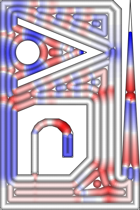
We first evaluate the accuracy of different beading schemes in terms of the relative amount of the overfill and underfill. We construct the over- and underfill area by comparing the shapes covered by each extrusion move with each other and with the total shape of the boundary polygons. (For implementation details see Appendix C.) This results in polygonal shapes such as visualized in the top half of Fig. 17: there are orange shapes where the beads overlap and azure shapes in the voids in between the beads. We compare the total area in of these overfill and underfill shapes to the total area of the boundary for each sample in the data set and report the average percentages in Fig. 18(a). The inward distributed scheme has a calculated overfill of and an underfill of . This is lower compared to the uniform scheme, which results in overfill and underfill in the data set.




6.1.2 Uniformity
We visualize the bead widths resulting from the different schemes in the bottom of Fig. 17. We binned the toolpaths into width bins at increments and determine the total toolpath length pertaining to each bin. From these statistics we calculate the mean and standard deviation and report them in Fig. 18(d). We found that the mean width of the inward and evenly distributed schemes is close to the preferred bead width of , while their standard deviation is lower than for the centered and constant bead count scheme. These results show that, while causing less overfill and underfill, inwards distributed and evenly distributed schemes deviate less or less often from the preferred bead width compared to the other schemes.
6.1.3 Print time
The total time it takes to print a part is influenced not only by our back pressure compensation scheme, but also by the geometry of the toolpaths. In order to separate these effects we report on the total print time when using back pressure compensation and when using a constant (maximum) movement speed in Fig. 18(b). We estimate print times using a simulation of the Marlin firmware using the default movement settings of the setup described in Section 5.2. While the idealized print time is predominantly determined by the total toolpath length, the print time using back pressure compensation is predominantly determined by the occurrence of wide beads, because they have a reduced the flow in . Because of acceleration constraints imposed by the hardware the maximum movement speed is not reached near sharp corners. We therefore also report on the angles of the bends in the toolpaths in Fig. 18(e). Furthermore, the print time is negatively affected by discontinuities in the extrusion process. Between extrusions the printer needs to stop extrusion, travel to the next extrusion path and restart the extrusion process, which may introduce defects and incurs extra print time. For closed polygonal toolpaths we can start anywhere within the path, so we can optimize the starting location so as to minimize the travel time. We therefore report both on the open and closed path count in Fig. 18(c).
6.1.4 Computational performance
Fig. 18(f) plots the computation time against the vertex count of the layer for the full data set, comparing the uniform technique implemented using Clipper [43] to our framework with the inward distributed scheme. For polygonal shapes with as many as vertices, the computation for both approaches is less than 1 second, with our method being approximately five times that of the uniform technique. These results could be improved upon by utilizing the locality inherent in our algorithms for parallelization on the GPU.
The computational complexity is limited by the generation of the Voronoi Diagram, which is , where is the number of vertices in the input shape. The other steps in our framework have a complexity of , where is the number of elements in the ST. Therefore, the total running time of our algorithm is . Results in Fig. 18(f) confirm that both our framework and the uniform technique have an expected running time of approximately seconds.
6.2 Comparison of beading schemes
We can see from Fig. 17(a)(top) and 18(a) that the uniform technique causes a lot of overfills and underfills: on average of the total target area is covered by underfill and likewise for overfill. To our knowledge, the uniform beading scheme, as well as the outer beading scheme, is of little use to FDM printers.
The constant bead count scheme effectively deals with underfills, but generates orders of magnitude more overfills compared to the other schemes. Also, the scheme comes at the cost of greatly varying bead widths and an average bead width that is not close to the preferred bead width. Note that most overfill areas occur near regions of alternating bead width. While the scheme results in short toolpaths, as indicated by the idealized print time, it also results in a wide range of bead widths, which cause the back pressure compensation print time to be very large. See Fig. 18. For an input outline shape which contains both very small and very large features, the constant bead count scheme produces bead widths which can fall outside of the range of manufacturable bead widths. Moreover the centrality marking is not robust against small perturbations in the outline; adding a small chamfer in a corner causes the unmarked ST to be very small at that location, which results in tiny bead widths. See top right of Fig. 17(b).
In Fig. 17(c) we can see that the centered beading scheme effectively deals with overfill and produces desired bead widths in all locations, except for the extrusion paths in the center, where the bead widths range between and . However, it does produce some narrow underfill regions. Compared to the uniform technique the centered technique increases the (open) path count, but considerably reduces over- and underfill and decimates the number of toolpath angles below . See Fig. 18.
However, according to Fig. 18(d) the centered scheme exhibits a wider range of bead widths than the distributed schemes: the standard deviation of the bead widths in the centered scheme is approximately , while that of the distributed schemes is approximately .11 1 Although the standard deviation of the inward distributed scheme is slightly higher than that of the evenly distributed scheme, the mean absolute deviation is lower (i.e. versus ), because its distribution is more peaked. Moreover, because the quantization operator rounds to the nearest number of beads, in the worst case where we switch from a single to two beads the widths switch from to , which is a considerably smaller range than in the centered scheme. We therefore conclude that the distributed schemes exhibit a lower bead width variation and lower (open) path count compared to the centered scheme.
Figures 13, 17(d) and 17(e) show that in the inward distributed scheme the outer toolpaths have the preferred width more often than in the evenly distributed scheme, which means that the outline accuracy of the inward distributed beading is less affected by inaccuracies in the adaptive width control system. Furthermore, we find that compared to evenly distributed, the inward distributed scheme produces less corners with angles above and less overfill, because the area of influence that bead count transitions have is limited in the inward distributed scheme. Thus the inward distributed scheme prevents over- and underfill, generates smooth toolpaths with more homogeneous width and affects smaller more centered parts of the print than the other schemes, while incurring little to no extra print time.
6.3 Limitations
Because the performance of the various toolpathing techniques depends on the geometry of a model, they have ramifications for the practice of design for additive manufacturing. Because the naive method produces under- or overfill for parts of an outline with a constant diameter it is best practice to design a model such that horizontal cross-sections have a feature diameter of an even integer multiple of the bead width. For the centerscheme and for the current state of the art one should only avoid parts for which in order to avoid underfill. For the distributed schemes however, there is no diameter at which the framework produces under- or overfill for a part with a constant diameter . The design consideration therefore reduces to limiting the diameter of your parts to be within the range , where is a configurable parameter when using the widening meta-scheme.
The default limit bisector angle ensures that we don’t employ transitioning in shallow wedge regions, which would result in a lot of short odd single bead polylines, which would break up the semi-continuous nature of polygonal extrusion paths; corresponds to long segments and under-/overfill areas of . However, future work might be aimed at reducing under-/overfill in regions with a low bisector angle without the introduction of short single polyline extrusion segments. If the over-/underfill problem is also solved for non-significant regions we might be able to increase and reduce the discontinuity introduced by short extrusion segments.
Another limitation of our method is that in a location with locally maximal the odd bead count will result in a single polyline extrusion segment consisting of only a single point. This can be viewed in the bottom right of Fig. 17(e) for example. In order to print such a dot, we make it into a long extrusion segment, with an altered width such that the total volume remains correct. A more principled way of dealing with such a situation remains future work.
Finally it should be noted that although our framework can accurately emulate the constant bead count approach by Ding et al. 2016, its emulation of the centered approach by Jin et al. 2017a is imperfect. The transitions resulting from out framework introduce sharper corners and there is more width variation in those corners. Whereas the width of the connecting segment in the approach by Jin et al. 2017a is the preferred width , the bead widths closer to the center resulting from our framework will be twice the local radius, which is larger than . However, this inflated bead width variation is expected to have an insignificant impact on the measured bead width variation.
6.4 Applications
Toolpaths with varying width is particularly meaningful for narrow parts, since there the negative effect of under- and overfill is more pronounced than in wide parts. In extreme cases, thin features will not be filled at all. Therefore, our framework, while working for wide parts as well, shows most of its potential for objects which contain thin parts.
Figure 19 collectively shows the application of the proposed inward distributed scheme for various types of 3D model, including both thin parts (architectural models, casings, embossed text, gears and microstructures) and wide parts (Fig. 19(b)) and organic shapes (Fig. 19(c))).
For architectural models and casings, preventing over- and underfill is expected to make them stronger. For embossed text, preventing underfill reduces the various holes in the top surfaces, which is detrimental to the visual quality of those top surfaces. For gears and similar mechanical parts that are designed with finite element analysis, the less variation in extrusion widths is closer to the assumptions under fast analysis (e.g. using homogenization [44]).
Of particular interest are microstructures that could be uniquely fabricated by 3D printing. For example, topology optimized bone-like structures [45] contain filaments of varying thickness that follow a varying stress direction (Fig. 19(g)). An angled Gyroid structure with uniform thickness also results in outline shapes with varying width (Fig. 19(h)). These structures are accurately densely filled using our framework. Another class of microstructures consists of parameterized patterns with varying thickness to achieve functional gradation. Figure 19(i) shows the contour-parallel toolpaths with varying width of a hexagonal grid neatly switches between different bead counts over the volume, preventing the jagged moves a direction-parallel toolpaths would create for such a case [1].


7 Conclusion
In this paper we have introduced a framework for computing contour-parallel toolpaths employing adaptive bead width in order to minimize underfill and overfill areas. We introduced beading schemes which improve on the state of the art, and we have introduced a back pressure compensation method for accurate fabrication of adaptive width.
Our framework is flexible, demonstrated by the several beading schemes which emulate existing techniques. The computation times of our framework are on par with the state-of-the-art library for performing offsets of non-adaptive bead width. Our framework is stable: small local changes in the outline shape cause only small changes in the toolpath.
Compared to the state of the art, the inward distributed beading scheme reduces the amount of beads with a width deviating extremely from the preferred bead width by changing the width of several beads near the center instead of only the center-most bead. It is therefore expected to limit the impact of varying the bead width in terms of production accuracy and homogeneity of material properties, which in turn is helpful to efficiently simulate an FDM manufactured part.
The proposed beading scheme greatly improves the process planning for parts with thin contours, which often occur for example in architectural models, prototypes for casings or microstructures. Meanwhile it leaves most of the toolpaths the same as the uniform width technique in large features, meaning that existing studies which relate process parameters with mechanical properties of the print are still applicable. Compared to the naive approach of constant width toolpaths our beading scheme is expected to improve the stiffness, dimensional accuracy and visual qualities of the manufactured model. It is expected that as distributed beading schemes are implemented in commercial software packages and bead width variation control become commonplace, the practice of design for additive manufacturing can disregards some of the nozzle size considerations.
The presented framework is open source available at
github.com/Ultimaker/libArachne
References
References
- Bates et al. [2018] S. R. Bates, I. R. Farrow, R. S. Trask, Compressive behaviour of 3D printed thermoplastic polyurethane honeycombs with graded densities, Materials & Design 162 (2018) 130–142, doi:10.1016/j.matdes.2018.11.019.
- Al-Ketan et al. [2018] O. Al-Ketan, R. Rowshan, R. K. Abu Al-Rub, Topology-mechanical property relationship of 3D printed strut, skeletal, and sheet based periodic metallic cellular materials, Additive Manufacturing 19 (2018) 167–183, doi:10.1016/j.addma.2017.12.006.
- Maskery et al. [2018] I. Maskery, L. Sturm, A. O. Aremu, A. Panesar, C. B. Williams, C. J. Tuck, R. D. Wildman, I. A. Ashcroft, R. J. M. Hague, Insights into the mechanical properties of several triply periodic minimal surface lattice structures made by polymer additive manufacturing, Polymer 152 (2018) 62–71, doi:10.1016/j.polymer.2017.11.049.
- Zegard and Paulino [2016] T. Zegard, G. H. Paulino, Bridging topology optimization and additive manufacturing, Structural and Multidisciplinary Optimization 53 (1) (2016) 175–192, ISSN 1615-1488, doi:10.1007/s00158-015-1274-4.
- Wu et al. [2019] J. Wu, W. Wang, X. Gao, Design and Optimization of Conforming Lattice Structures, IEEE Transactions on Visualization and Computer Graphics (2019) 1–14URL http://arxiv.org/abs/1905.02902.
- Cheng et al. [2019] L. Cheng, J. Bai, A. C. To, Functionally graded lattice structure topology optimization for the design of additive manufactured components with stress constraints, Computer Methods in Applied Mechanics and Engineering 344 (2019) 334–359, doi:10.1016/j.cma.2018.10.010.
- Ding et al. [2016] D. Ding, Z. Pan, D. Cuiuri, H. Li, N. Larkin, Adaptive path planning for wire-feed additive manufacturing using medial axis transformation, Journal of Cleaner Production 133 (2016) 942–952, doi:10.1016/j.jclepro.2016.06.036.
- Xiong et al. [2019] Y. Xiong, S.-I. Park, S. Padmanathan, A. G. Dharmawan, S. Foong, D. W. Rosen, G. S. Soh, Process planning for adaptive contour parallel toolpath in additive manufacturing with variable bead width, The International Journal of Advanced Manufacturing Technology doi:10.1007/s00170-019-03954-1.
- Jin et al. [2017a] Y. Jin, J. Du, Y. He, Optimization of process planning for reducing material consumption in additive manufacturing, Journal of Manufacturing Systems 44 (2017a) 65–78, doi:10.1016/j.jmsy.2017.05.003.
- Ultimaker [2019] Ultimaker, Ultimaker Cura 4.2.1 software, URL https://ultimaker.com/software/ultimaker-cura, 2019.
- Livesu et al. [2017] M. Livesu, S. Ellero, J. Martínez, S. Lefebvre, M. Attene, From 3D models to 3D prints: an overview of the processing pipeline, Computer Graphics Forum 36 (2) (2017) 537–564, doi:10.1111/cgf.13147.
- N. Turner et al. [2014] B. N. Turner, R. Strong, S. A. Gold, A review of melt extrusion additive manufacturing processes: I. Process design and modeling, Rapid Prototyping Journal 20 (3) (2014) 192–204, doi:10.1108/RPJ-01-2013-0012.
- Ahn et al. [2002] S. H. Ahn, M. Montero, D. Odell, S. Roundy, P. K. Wright, Anisotropic material properties of fused deposition modeling ABS, Rapid Prototyping Journal 8 (4) (2002) 248–257, doi:10.1108/13552540210441166.
- Kuipers et al. [2019] T. Kuipers, J. Wu, C. C. L. Wang, CrossFill: Foam Structures with Graded Density for Continuous Material Extrusion, Computer-Aided Design 114 (2019) 37–50, doi:10.1016/j.cad.2019.05.003.
- Han et al. [2002] W. Han, M. A. Jafari, S. C. Danforth, A. Safari, Tool Path-Based Deposition Planning in Fused Deposition Processes , Journal of Manufacturing Science and Engineering 124 (2) (2002) 462–472, doi:10.1115/1.1455026.
- Steuben et al. [2016] J. C. Steuben, A. P. Iliopoulos, J. G. Michopoulos, Implicit slicing for functionally tailored additive manufacturing, Computer-Aided Design 77 (2016) 107–119, doi:10.1016/j.cad.2016.04.003.
- Zhao et al. [2016] H. Zhao, B. Chen, F. Gu, Q.-X. Huang, J. Garcia, Y. Chen, C. Tu, B. Benes, H. Zhang, D. Cohen-Or, Connected fermat spirals for layered fabrication, ACM Transactions on Graphics 35 (4) (2016) 1–10, doi:10.1145/2897824.2925958.
- Jin et al. [2017b] Y. Jin, Y. He, G. Fu, A. Zhang, J. Du, A non-retraction path planning approach for extrusion-based additive manufacturing, Robotics and Computer-Integrated Manufacturing 48 (2017b) 132–144, doi:10.1016/j.rcim.2017.03.008.
- Held and Spielberger [2009] M. Held, C. Spielberger, A smooth spiral tool path for high speed machining of 2D pockets, Computer-Aided Design 41 (7) (2009) 539–550, doi:10.1016/j.cad.2009.04.002.
- Huang et al. [2017] N. Huang, R. Lynn, T. Kurfess, Aggressive Spiral Toolpaths for Pocket Machining Based on Medial Axis Transformation, Journal of Manufacturing Science and Engineering 139 (5), doi:10.1115/1.4035720.
- McMains et al. [2000] S. McMains, J. Smith, J. Wang, C. Sequin, S. Carlo, Layered manufacturing of thin-walled parts, in: ASME Design Engineering Technical Conference, Baltimore, Maryland, Citeseer, 2000.
- Jin et al. [2013] Y. A. Jin, Y. He, J. Z. Fu, An Adaptive Tool Path Generation for Fused Deposition Modeling, in: Advanced Materials Research, vol. 819, 7–12, doi:10.4028/www.scientific.net/amr.819.7, 2013.
- Ding et al. [2014] D. Ding, Z. Pan, D. Cuiuri, H. Li, A tool-path generation strategy for wire and arc additive manufacturing, International Journal of Advanced Manufacturing Technology 73 (1-4) (2014) 173–183, doi:10.1007/s00170-014-5808-5.
- Cox et al. [1994] J. J. Cox, Y. Takezaki, H. R. P. Ferguson, K. E. Kohkonen, E. L. Mulkay, Space-filling curves in tool-path applications, Computer-Aided Design 26 (3) (1994) 215–224, doi:https://doi.org/10.1016/0010-4485(94)90044-2.
- Griffiths [1994] J. G. Griffiths, Toolpath based on Hilbert’s curve, Computer-Aided Design 26 (11) (1994) 839–844, doi:10.1016/0010-4485(94)90098-1.
- Shaikh et al. [2016] S. Shaikh, N. Kumar, P. K. Jain, P. Tandon, Hilbert curve based toolpath for FDM process, in: CAD/CAM, Robotics and Factories of the Future, Lecture Notes in Mechanical Engineering, Springer, 751–759, doi:10.1007/978-81-322-2740-3_72, 2016.
- Kao and Prinz [1998] J.-h. Kao, F. B. Prinz, Optimal motion planning for deposition in layered manufacturing, in: Proceedings of DETC, vol. 98, Citeseer, 13–16, 1998.
- Jin et al. [2017c] Y. Jin, Y. He, J. Du, A novel path planning methodology for extrusion-based additive manufacturing of thin-walled parts, International Journal of Computer Integrated Manufacturing 30 (12) (2017c) 1301–1315, doi:10.1080/0951192X.2017.1307526.
- Moesen et al. [2011] M. Moesen, T. Craeghs, J. P. Kruth, J. Schrooten, Robust beam compensation for laser-based additive manufacturing, Computer-Aided Design 43 (8) (2011) 876–888, doi:10.1016/j.cad.2011.03.004.
- Behandish et al. [2019] M. Behandish, A. M. Mirzendehdel, S. Nelaturi, A Classification of Topological Discrepancies in Additive Manufacturing, Computer-Aided Design doi:10.1016/j.cad.2019.05.032.
- Eiamsa-ard et al. [2003] K. Eiamsa-ard, F. W. Liou, R. G. Landers, H. Choset, Toward automatic process planning of a multi-axis hybrid laser aided manufacturing system: skeleton-based offset edge generation, in: ASME 2003 International Design Engineering Technical Conferences and Computers and Information in Engineering Conference, American Society of Mechanical Engineers Digital Collection, 227–235, doi:10.1115/DETC2003/DAC-48726, 2003.
- Blum et al. [1967] H. Blum, et al., A transformation for extracting new descriptors of shape, Models for the perception of speech and visual form 19 (5) (1967) 362–380.
- Lee [1982] D.-T. T. Lee, Medial Axis Transformation of a Planar Shape, IEEE Transactions on Pattern Analysis and Machine Intelligence PAMI-4 (4) (1982) 363–369, doi:10.1109/TPAMI.1982.4767267.
- Chazelle and Incerpi [1984] B. Chazelle, J. Incerpi, Triangulation and shape-complexity, ACM Transactions on Graphics 3 (2) (1984) 135–152, doi:10.1145/357337.357340.
- Fournier and Montuno [1984] A. Fournier, D. Y. Montuno, Triangulating Simple Polygons and Equivalent Problems, ACM Transactions on Graphics 3 (2) (1984) 153–174, doi:10.1145/357337.357341.
- Schäling [2011] B. Schäling, The boost C++ libraries, Boris Schäling, 2011.
- Fortune [1987] S. Fortune, A sweepline algorithm for Voronoi diagrams, Algorithmica 2 (1) (1987) 153, doi:10.1007/BF01840357.
- Attali and Montanvert [1996] D. Attali, A. Montanvert, Modeling noise for a better simplification of skeletons, in: Proceedings of 3rd IEEE International Conference on Image Processing, vol. 3, IEEE, 13–16, doi:10.1109/ICIP.1996.560357, 1996.
- Sud et al. [2005] A. Sud, M. Foskey, D. Manocha, Homotopy-Preserving Medial Axis Simplification, in: Proceedings of the 2005 ACM Symposium on Solid and Physical Modeling, Association for Computing Machinery, 39–50, doi:10.1145/1060244.1060250, 2005.
- Kuipers et al. [2018] T. Kuipers, W. Elkhuizen, J. Verlinden, E. Doubrovski, Hatching for 3D prints: Line-based halftoning for dual extrusion fused deposition modeling, Computers & Graphics 74 (2018) 23–32, doi:10.1016/j.cag.2018.04.006.
- Ertay et al. [2018] D. S. Ertay, A. Yuen, Y. Altintas, Synchronized material deposition rate control with path velocity on fused filament fabrication machines, Additive Manufacturing 19 (2018) 205–213, doi:10.1016/j.addma.2017.05.011.
- Tronvoll et al. [2019] S. A. Tronvoll, S. Popp, C. W. Elverum, T. Welo, Investigating pressure advance algorithms for filament-based melt extrusion additive manufacturing: theory, practice and simulations, Rapid Prototyping Journal 25 (5) (2019) 830–839, doi:10.1108/RPJ-10-2018-0275.
- Johnson [2017] A. Johnson, Clipper 6.4.2 - an open source freeware library for clipping and offsetting lines and polygons, 2017.
- Liu and Shapiro [2016] X. Liu, V. Shapiro, Homogenization of material properties in additively manufactured structures, Computer-Aided Design 78 (2016) 71 – 82, doi:https://doi.org/10.1016/j.cad.2016.05.017.
- Wu et al. [2018] J. Wu, N. Aage, R. Westermann, O. Sigmund, Infill Optimization for Additive Manufacturing – Approaching Bone-Like Porous Structures, IEEE Transactions on Visualization and Computer Graphics 24 (2) (2018) 1127–1140, doi:10.1109/TVCG.2017.2655523.
Appendix A Edge discretization
We calculate the location of the boundary between a significant and nonsignificant portion of an edge analytically. For example, the parabolic MAT edge generated from the outline vertex and an outline segment aligned with the X-axis follows and . We can determine the significant portion by evaluating , which is . Similarly, a MAT edge generated from two vertices at and follows and . The boundaries of significance are given by . From these we can derive the locations . These specific cases can easily be transformed into all possible cases using scaling and rotation operations.
Appendix B Data set
The data set we tested on was a custom selected set of open source 3D models found on the internet which was selected to cover a broad range of different types of application and geometry. Applications range from prototypes, to fixtures and mechanical end-use parts. The geometry covers a wide range including thin filaments, smooth surfaces, organic shapes, chamfered shapes, small shapes and large shapes. The models are described in Table 2.
| Model Name | Author |
|---|---|
| AirCasting Air Monitor Casing | HabitatMap |
| Air hose splitter | frizinko |
| Al Hamra Tower | TurnerConstructionCompany |
| canon NP-E3 battery cap | kosuyoung |
| David | Thunk3D |
| Deck Assembly Tool | PSomeone |
| Ender 3 Cable Chain | johnniewhiskey |
| Ergonomic Hacksaw Handle | mmOne |
| Gap measurement tool | ravm84 |
| G-Clamp fully printable | johann517 |
| Gyroid | Tim Kuipers |
| 3D Printable Jet Engine | CATIAV5FTW |
| Lawn Mower Throttle Replacement | Spammington |
| OpenRC F1 Internal gear box mod | intoxikated |
| PCB Test Fixture | JMadison |
| Pioneer Radio Holder for Ford Focus | Perugino |
| Replicator Dual Fan Mount | aubenc |
| Atuador versão 2 * actuator version 2 | Caroline Holanda |
| TE Pocket Operator Hard case | Salvation76 |
| Screw sizer | Pierrolalune63 |
| Bone-like optimized infill | Jun Wu |
| Two-Story Spec House | pwc-phil |
Appendix C Accuracy calculation
In order to estimate the overfill and underfill, we need to accurately calculate the area covered by a single extrusion path. If we would simply use an isosceles trapezoidal area, we would get overfill artifacts at corners in the toolpath (Fig. 20(a)). We therefore use a semi-circle (Fig. 20(b)) with a diameter equal to the starting width in the one end of each segment, and exclude it at the other end, because it will be included in the next segment. For polyline extrusion paths which are not closed, we also include the semi-circle of the destination location (Fig. 20(c)).
Using boolean operations we can obtain the polygonal regions for overfill and those for underfill. In order to deal with rounding errors we perform a morphological close of , before calculating the total area in . We also calculate regions which are covered thrice by different extrusion segments and add twice its area to the total overfill area amount.