跳到论文正文
W Papers独立论文阅读器 arXiv:2004.13360 论文正文 计算阅读时间 · 0%
引用这篇论文根据当前论文元数据生成,正式投稿前建议核对。


License: arXiv.org perpetual non-exclusive license
arXiv:2004.13360v2 [math.AP] 28 May 2020

Propagation phenomena with nonlocal diffusion in presence of an obstacle

Julien Brasseur Address: École des Hautes Études en Sciences Sociales, PSL Research University, CNRS, Centre d’Analyse et de Mathématique Sociales, Paris, France Email address: julien.brasseur@ehess.fr, julienbrasseur@wanadoo.fr and Jérôme Coville Address: BioSP, INRA, 84914, Avignon, France Email address: jerome.coville@inra.fr
Abstract.

We consider a nonlocal semi-linear parabolic equation on a connected exterior domain of the form ℝN∖K\mathbb{R}^{N}\setminus K, where K⊂ℝNK\subset\mathbb{R}^{N} is a compact “obstacle”. The model we study is motivated by applications in biology and takes into account long range dispersal events that may be anisotropic depending on how a given population perceives the environment. To formulate this in a meaningful manner, we introduce a new theoretical framework which is of both mathematical and biological interest. The main goal of this paper is to construct an entire solution that behaves like a planar travelling wave as t→−∞t\to-\infty and to study how this solution propagates depending on the shape of the obstacle. We show that whether the solution recovers the shape of a planar front in the large time limit is equivalent to whether a certain Liouville type property is satisfied. We study the validity of this Liouville type property and we extend some previous results of Hamel, Valdinoci and the authors. Lastly, we show that the entire solution is a generalised transition front.

2010 Mathematics Subject Classification
35J60

1. Introduction

Since the seminal works of Fisher [40], Kolmogorov, Petrovskii and Piskunov [50] on the propagation of advantageous genes in an homogeneous population, reaction-diffusion models have been extensively used to study the complex dynamics arising in nature [11, 21, 47, 48, 58, 65]. One of the main success of this type of modelling is the notion of “travelling waves” that has emerged from it, which has provided a rich and flexible theoretical framework to analyse the underlying dynamics of the problem considered.

In the past two decades, reaction-diffusion models involving more realistic descriptions of spatial interactions as well as of the environment have been considered to analyse a wide range of problems from ecology [48, 49, 65, 77], combustion theory [45, 46, 78] or phase transition in heterogeneous medium [33, 35]. This has considerably increased our understanding of the impact of the time and spatial heterogeneities of the environment on propagation phenomena. In turn, this profusion of work has led to the introduction of new notions of travelling waves generalising the traditional notion of planar wave and reflecting the essential properties of the environment [8, 10, 12, 13, 14, 16, 49, 56, 59, 63, 72, 77, 83]. In particular, notions such as pulsating fronts, random fronts or conical (or curved) fronts have been introduced to analyse propagation phenomena occurring in time and/or space periodic environments [8, 13, 57, 59, 83], or random ergodic environments [56, 63, 72], or to study propagation phenomena with some geometrical constraints [6, 16, 62]. It turns out that almost all of these new notions fall into the definition of generalised transition wave recently introduced by Berestycki and Hamel in [9], see also [10, 43].

It is worth mentioning that the complexity of propagation phenomena may come from either heterogeneous interactions (heterogeneous diffusion and reaction) or the geometry of the domain where the equation is defined (cylinder with rough boundary or domain with a complex structure). In the latter case, new phenomena are observed such as the pinning of fronts. We point the interested reader to [11, 60, 83] and references therein for a more thorough description of the state of the art on propagation phenomena in the context of reaction-diffusion equations.

Propagation phenomena can also be observed using other types of models, in particular nonlocal models that take into account long range dispersal phenomena (which are commonly observed in ecology, see [3, 4, 20, 23]). For example, planar fronts [2, 5, 22, 25, 30, 31, 34], pulsating fronts [32, 38, 68, 76] and generalised transition waves [15, 54, 73, 74, 75] have been constructed for integro-differential models of the form

(1.1) ∂tu⁡(t,x)=𝒥∗u⁡(t,x)−u⁡(t,x)+f⁡(t,x,u⁡(t,x))​ for ​(t,x)∈ℝ×ℝN,\partial_{t}u(t,x)=\mathcal{J}\ast u(t,x)-u(t,x)+f(t,x,u(t,x))\,{\mbox{ for }}(t,x)\in\mathbb{R}\times\mathbb{R}^{N},

where ff is a classical bistable or monostable nonlinearity, 𝒥\mathcal{J} is a nonnegative probability density function and ∗\ast is the standard convolution operator given by

𝒥∗u⁡(x):=∫ℝN𝒥⁡(x−y)​u​(y)​𝑑y.\mathcal{J}\ast u(x):=\int_{\mathbb{R}^{N}}\mathcal{J}(x-y)\hskip 0.50003ptu(y)\hskip 1.00006pt\mathrm{d}y.

However, to the best of our knowledge, there are no results dealing with the impact of the geometry on the large time dynamics of such nonlocal semi-linear equation, and only linear versions of (1.1) seem to have been considered, see [28, 29].

In the spirit of the pioneer work of Berestycki, Hamel and Matano [12], we analyse here the effect of the geometry of the domain on the propagation phenomena for an adapted version of (1.1) on exterior domains. Precisely, given a compact set K⊂ℝNK\subset\mathbb{R}^{N} with nonempty interior such that the exterior domain Ω:=ℝN∖K\Omega:=\mathbb{R}^{N}\setminus K is connected, we are interested in the properties and large time behaviour of the entire solutions uu to the following nonlocal semi-linear parabolic problem

(P) ∂tu=L​u+f⁡(u)​ a.e. in ​ℝ×Ω¯,\displaystyle\partial_{t}u=Lu+f(u)\,{\mbox{ a.e. in }}\mathbb{R}\times\overline{\Omega},

where LL is the nonlocal diffusion operator given by

L​u​(x):=∫ℝN∖KJ⁡(δ⁡(x,y))​(u⁡(y)−u⁡(x))​𝑑y.\displaystyle Lu(x):=\int_{\mathbb{R}^{N}\setminus K}J(\delta(x,y))\hskip 0.50003pt(u(y)-u(x))\hskip 1.00006pt\mathrm{d}y.

Here, JJ is a nonnegative kernel, ff is a “bistable” nonlinearity and δ:Ω¯×Ω¯→[0,∞)\delta:\overline{\Omega}\times\overline{\Omega}\to[0,\infty) is a distance on Ω¯\overline{\Omega} that behaves locally like the Euclidean distance (precise assumptions on JJ, ff and δ\delta will be given later on, see Subsection 1.3).

The problem (P) can be seen as a nonlocal version of the reaction-diffusion problem studied by Berestycki, Hamel and Matano in [12], namely

{∂tu=Δ​u+f⁡(u)in ​ℝ×Ω,∇u⋅ν=0on ​ℝ×∂Ω.\displaystyle\left\{\begin{array}[]{rl}\partial_{t}u=\Delta u+f(u)&\text{in }\mathbb{R}\times\Omega,\\ \nabla u\cdot\nu=0&\text{on }\mathbb{R}\times\partial\Omega.\end{array}\right.

There, they show that for any unit vector e∈𝕊N−1e\in\mathbb{S}^{N-1} (where 𝕊N−1\mathbb{S}^{N-1} denotes the unit sphere of ℝN\mathbb{R}^{N}), there exists a generalised transition wave in the direction ee solution to (1), i.e. for any e∈𝕊N−1e\in\mathbb{S}^{N-1}, there exists an entire solution, u⁡(t,x)u(t,x), to (1) defined for all t∈ℝt\in\mathbb{R} and all x∈Ω¯x\in\overline{\Omega} that satisfies 0<u⁡(t,x)<10<u(t,x)<1 for all (t,x)∈ℝ×Ω¯(t,x)\in\mathbb{R}\times\overline{\Omega} and such that

|u⁡(t,x)−ϕ⁡(x⋅e+c​t)|​⟶t→−∞​0​ uniformly in ​x∈Ω¯,|u(t,x)-\phi(x\cdot e+ct)|\underset{t\to-\infty}{\longrightarrow}0\,{\mbox{ uniformly in }}x\in\overline{\Omega},

where (ϕ,c)(\phi,c) is a planar travelling wave of speed c>0c>0. That is, (ϕ,c)(\phi,c) is the unique (up to shift) increasing solution to

{c​ϕ′=ϕ′′+f⁡(ϕ)​ in ​ℝ,limz→+∞ϕ(z)=1,limz→−∞ϕ(z)=0.\displaystyle\left\{\begin{array}[]{l}c\,\phi^{\prime}=\phi^{\prime\prime}+f(\phi)\text{ in }\mathbb{R},\\ \displaystyle\lim_{z\to+\infty}\phi(z)=1,\,\lim_{z\to-\infty}\phi(z)=0.\end{array}\right.

Moreover, they prove that there exists a classical solution, u∞u_{\infty}, to

{Δ​u∞+f⁡(u∞)=0in ​Ω¯,∇u∞⋅ν=0on ​∂Ω,0<u∞⩽1in ​Ω¯,u∞​(x)→1as ​|x|→+∞,\displaystyle\left\{\begin{array}[]{rl}\Delta u_{\infty}+f(u_{\infty})=0&\text{in }\overline{\Omega},\\ \nabla u_{\infty}\cdot\nu=0&\text{on }\partial\Omega,\\ 0<u_{\infty}\leqslant 1&\text{in }\overline{\Omega},\\ u_{\infty}(x)\to 1&\text{as }|x|\to+\infty,\end{array}\right.

which they show corresponds to the large time limit of u⁡(t,x)u(t,x) in the sense that

|u⁡(t,x)−u∞​(x)​ϕ​(x⋅e+c​t)|​⟶t→∞​0​ uniformly in ​x∈Ω¯.|u(t,x)-u_{\infty}(x)\hskip 1.00006pt\phi(x\cdot e+ct)|\underset{t\to\infty}{\longrightarrow}0\,{\mbox{ uniformly in }}x\in\overline{\Omega}.

In addition, they were able to classify the solutions u∞u_{\infty} to (1) with respect to the geometry of KK. Precisely, they proved that if the obstacle KK is either starshaped or directionally convex (see [12, Definition 1.2]), then the solutions u∞u_{\infty} to (1) are actually identically equal to 11 in the whole set Ω¯\overline{\Omega}. This remarkable rigidity property was further extended to more complex obstacles by Bouhours in [17] who showed a sort of “stability” of this result with respect to small regular perturbations of the obstacle. Yet, this phenomenon does not hold in general. Indeed, Berestycki et al. [12] proved that when the domain is no longer starshaped nor directionally convex but merely simply connected (see [12]), then (1) admits nontrivial solutions with 0<u∞<10<u_{\infty}<1 in Ω¯\overline{\Omega}, thus implying that the disturbance caused by the obstacle may remain forever depending on the geometry of KK.

Our main objective in this article is to construct such an entire solution for the problem (P) and to study its main properties with respect to the geometry of the domain.

1.1. Biological motivation

Before stating our main results, let us first discuss the relevance of this type of model. To this end, let us go back to the very description of population dispersal. For it, let us denote by u⁡(t,x)u(t,x) the density of the population at time tt and location xx. Moreover, let us discretize uniformly the domain Ω\Omega into small cubes of volume |Δ​xi||\Delta x_{i}| centered at points xi∈Ωx_{i}\in\Omega, and the time into discrete time steps Δ​t\Delta t. Then, following Huston et al. [44], we can describe the evolution of the population in terms of the exchange of individuals between sites. Namely, for a site xix_{i}, the total number of individuals N⁡(t,xi)N(t,x_{i}) will change during the time step Δ​t\Delta t according to

N⁡(t+Δ​t,xi)−N⁡(t,xi)Δ​t=Ni←−Ni→Δ​t,\displaystyle\frac{N(t+\Delta t,x_{i})-N(t,x_{i})}{\Delta t}=\frac{N_{i\leftarrow}-N_{i\to}}{\Delta t},

where Ni←N_{i\leftarrow} and Ni→N_{i\to} denote the total number of individuals reaching and leaving the site xix_{i}, respectively. Since N⁡(t,xi)=u⁡(t,xi)​|Δ​xi|N(t,x_{i})=u(t,x_{i})|\Delta x_{i}|, this can be rewritten

u⁡(t+Δ​t,xi)−u⁡(t,xi)Δ​t|Δ​xi|=γ​|Δ​xi|​∑j=−∞+∞(𝒥⁡(xi,xj)​u​(t,xj)−𝒥⁡(xj,xi)​u​(t,xi))​|Δ​xj|,\frac{u(t+\Delta t,x_{i})-u(t,x_{i})}{\Delta t}|\Delta x_{i}|=\gamma\hskip 1.00006pt|\Delta x_{i}|\sum_{j=-\infty}^{+\infty}\big(\mathcal{J}(x_{i},x_{j})\hskip 0.50003ptu(t,x_{j})-\mathcal{J}(x_{j},x_{i})\hskip 0.50003ptu(t,x_{i})\big)|\Delta x_{j}|,

where 𝒥⁡(xi,xj)\mathcal{J}(x_{i},x_{j}) denotes the rate of transfer of individuals from the site xix_{i} to the site xjx_{j} and γ\gamma denotes a dispersal rate (or diffusion coefficient).

In ecology, understanding the structure of the rate of transfer 𝒥⁡(xi,xj)\mathcal{J}(x_{i},x_{j}) is of prime interest as it is known to condition some important feature of the dispersal of the individuals [26, 51, 61, 70]. For example, this rate can reflect some constraints of the environment on the capacity of movement of the individuals [26, 27, 36, 42, 71] and/or incorporate important features that are biologically/ecologically relevant such as a dispersal budget [7, 44] or a more intrinsic description of the landscape such as its connectivity, fragmentation, anisotropy or other particular geometrical structure [1, 26, 36, 37, 69, 80, 81].

Here, we are particularly interested in the impact that the geometry of Ω\Omega can have on this rate. A natural assumption is to consider that 𝒥⁡(xi,xj)\mathcal{J}(x_{i},x_{j}) depends on the “effective distance” between xix_{i} and xjx_{j}. The perception of the environment being a characteristic trait of a given species (as observed in [41]), this notion of “effective distance” will then change depending on the species considered.

Let us consider, for instance, an habitat consisting of a uniform field with, in the middle of it, a circular pond, e.g. Ω:=ℝ2∖B1¯\Omega:=\mathbb{R}^{2}\setminus\overline{B_{1}} where B1B_{1} denotes the unit disk of ℝ2\mathbb{R}^{2}. One can then imagine that, for some species having a high dispersal capacity (as, for example, bees [66]), the pond will not be considered as an obstacle in the sense that it does not affect their displacement (since the individuals can easily “jump” from one side of the pond to another). On the contrary, for other species, such as many land animals, this pond will actually be seen as a physical dispersal barrier. Whence, to go from one side of the pond to another they will have to circumvent it. So, in this case, the metric considered to evaluate this “effective distance” has to reflect such type of behaviour (see e.g. [71] for an illustrative example).
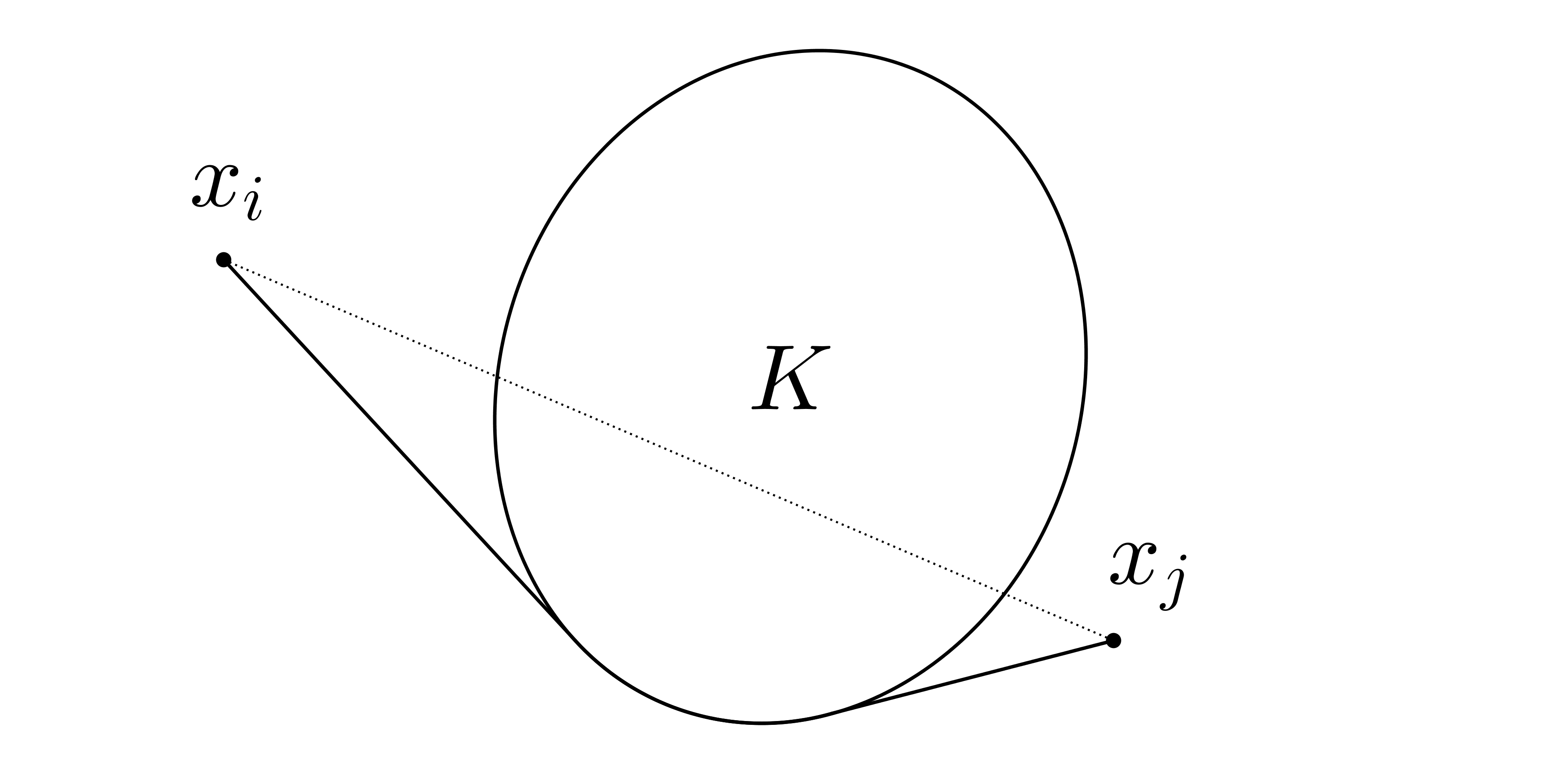
Refer to caption
Figure 1. The geodesic distance (continuous line)

and the Euclidean distance (dashed line) between xi,xj∈ℝN∖Kx_{i},x_{j}\in\mathbb{R}^{N}\setminus K.

A way to understand the impact of the landscape on the movement of the individuals is to use a “least cost path” modelling [1, 36, 79]. The metric related to this geographic concept can then serve as a prototype for the metric used to evaluate 𝒥⁡(xi,xj)\mathcal{J}(x_{i},x_{j}). The idea behind the “least cost path” concept is to assign to each path taken to join one site to another some costs related to a predetermined constraint and try to minimize the costs. This notion can then be related to the notion of geodesic path on a smooth surface where the costs then reflect some geometrical aspect of the landscape. Following this idea, it is then natural to consider the “effective distance” as some geodesic distance δ\delta reflecting how the geometry of the landscape is perceived by the species considered and to take 𝒥⁡(xi,xj)=J⁡(δ⁡(xi,xj))\mathcal{J}(x_{i},x_{j})=J(\delta(x_{i},x_{j})), where JJ is a function encoding the probability to make a jump of length δ⁡(xi,xj)\delta(x_{i},x_{j}). In the above example, the appropriate distance will then be either the standard Euclidean distance (i.e. δ⁡(xi,xj)=|xi−xj|\delta(x_{i},x_{j})=|x_{i}-x_{j}|) or the geodesic distance defined in the perforated domain Ω\Omega.

Since diffusion is classically accompanied by demographic variations (which we may suppose to be described by a nonlinear function ff of the density of population), by letting |Δ​xj|→0+|\Delta x_{j}|\to 0^{+} and Δ​t→0+\Delta t\to 0^{+}, we then formally get

∂tu⁡(t,x)=γ⁡(∫ΩJ⁡(δ⁡(x,y))​u​(t,y)​𝑑y−u⁡(t,x)​∫ΩJ⁡(δ⁡(y,x))​𝑑y)+f⁡(u⁡(t,x)),\partial_{t}u(t,x)=\gamma\left(\int_{\Omega}J(\delta(x,y))\hskip 0.50003ptu(t,y)\hskip 1.00006pt\mathrm{d}y-u(t,x)\int_{\Omega}J(\delta(y,x))\hskip 1.00006pt\mathrm{d}y\right)+f(u(t,x)),

which thereby yields equation (P), up to an immaterial constant γ\gamma.

It is worth mentioning that, although the description of the rate of transfer using a geodesic distance is well-known in the ecology community [36, 79], to our knowledge, this the first time that such concept has been formalised mathematically in the framework of nonlocal reaction-dispersal equations to describe the evolution of a population living in a domain and having a long distance dispersal strategy.

The mathematical framework we propose goes far beyond the situation we analyse here. Indeed, the model (P) is quite natural and well-posed as soon as a geodesic-type distance, which we will refer to as “quasi-Euclidean” (see Definition 1.2), can be defined on the domain Ω\Omega considered, allowing thus to handle domains with very complex geometrical structure (such graph trees, which are particularly pertinent in conservation biology for the help they can provide in the understanding of the impact of blue and green belts in urban landscapes [52, 84]). As we will see, our setting also allows to model an extremely wide class of biologically relevant “effective distances” (see Remark 1.5).

1.2. Notations and definitions

Before we set our main assumptions, we need to introduce some necessary definitions.

We begin with the metric framework on which we will work.

Definition 1.1.

Let x,y∈ℝNx,y\in\mathbb{R}^{N}. We call a path connecting xx to yy any continuous piecewise C1C^{1} function γ:[0,1]→ℝN\gamma:[0,1]\to\mathbb{R}^{N} with γ⁡(0)=x\gamma(0)=x and γ⁡(1)=y\gamma(1)=y and we denote by length⁡(γ)\mathrm{length}(\gamma) its length. The set of all such paths is denoted by H⁡(x,y)H(x,y).

Definition 1.2.

Let E⊂ℝNE\subset\mathbb{R}^{N}. A quasi-Euclidean distance on EE is a distance δ\delta on EE such that δ⁡(x,y)=|x−y|\delta(x,y)=|x-y| if [x,y]⊂E[x,y]\subset E and δ⁡(x,y)⩾|x−y|\delta(x,y)\geqslant|x-y| for all x,y∈Ex,y\in E. We denote by 𝒬⁡(E)\mathcal{Q}(E) the set of all quasi-Euclidean distances on EE.

Example 1.3.

The geodesic distance dEd_{E} on a set EE, defined by

dE​(x,y):={infγ∈H⁡(x,y)γ⊂E¯length⁡(γ) if ​x,y​ belong to the same connected component,+∞ otherwise,\displaystyle d_{E}(x,y):=\left\{\begin{array}[]{cl}\displaystyle\inf_{\gamma\in H(x,y)\atop\gamma\subset\overline{E}}\,\mathrm{length}(\gamma)&\text{ if }x,y\text{ belong to the same connected component},\\ +\infty&\text{ otherwise,}\end{array}\right.

is a nontrivial quasi-Euclidean distance. If dFd_{F} is the geodesic distance on a set F⊃EF\supset E, then its restriction dF​ E\mathchoice{{d_{F}\,\smash{\vrule height=5.55557pt,depth=1.27501pt}}_{\,E}}{{d_{F}\,\smash{\vrule height=5.55557pt,depth=1.27501pt}}_{\,E}}{{d_{F}\,\smash{\vrule height=3.88889pt,depth=0.85472pt}}_{\,E}}{{d_{F}\,\smash{\vrule height=2.77777pt,depth=1.44028pt}}_{\,E}} to E×EE\times E is another nontrivial example of quasi-Euclidean distance on EE. Moreover, since 𝒬⁡(E)\mathcal{Q}(E) is a convex set, one may obtain other examples of such distances by convex combination of the previous examples and/or the Euclidean distance.

Remark 1.4.

If EE is convex, then the Euclidean distance is the only quasi-Euclidean distance.

Remark 1.5.

Roughly speaking, a quasi-Euclidean distance can be interpreted as the length of a path connecting two points and which behaves locally like the Euclidean distance. In fact, the condition δ⁡(x,y)⩾|x−y|\delta(x,y)\geqslant|x-y| can be equivalently rephrased by saying that, for any two points x,y∈Ex,y\in E, there exists a path γ∈H⁡(x,y)\gamma\in H(x,y) (which is not compelled to stay in EE) connecting xx to yy and such that δ⁡(x,y)=length⁡(γ)\delta(x,y)=\mathrm{length}(\gamma). Biologically speaking, it provides a natural and flexible tool to model the “effective distance” between two locations. It can account for a wide range of situations, for example it can model a population whose individuals can jump through some obstacles (say small ones) and not through others (say large ones), or through portions of an obstacle, as well as all the intermediary situations.

Definition 1.6.

Let E⊂ℝNE\subset\mathbb{R}^{N} be a connected set and let δ∈𝒬⁡(E¯)\delta\in\mathcal{Q}(\overline{E}). Let J:[0,∞)→[0,∞)J:[0,\infty)\to[0,\infty) be a measurable function with |supp⁡(J)|>0|\mathrm{supp}(J)|>0. For any x∈E¯x\in\overline{E}, we define Π0​(J,x):={x}\Pi_{0}(J,x):=\{x\} and

Πj+1​(J,x):=⋃z∈Πj​(J,x)supp⁡(J⁡(δ⁡(⋅,z)))​ for any ​j⩾0.\Pi_{j+1}(J,x):=\bigcup_{z\in\Pi_{j}(J,x)}\!\!\mathrm{supp}\left(J(\delta(\cdot,z))\right)\,{\mbox{ for any }}j\geqslant 0.

We say that the metric space (E,δ)(E,\delta) has the JJ-covering property if

E¯=⋃j⩾0Πj​(J,x)​ for every ​x∈E¯.\overline{E}=\bigcup_{j\geqslant 0}\,\Pi_{j}(J,x)\,{\mbox{ for every }}x\in\overline{E}.
Remark 1.7.

If EE is a connected set and if δ\delta is the Euclidean distance, then the above property is automatically satisfied (see Proposition A.1 in the Appendix). Moreover, if E=ℝN∖KE=\mathbb{R}^{N}\setminus K for some compact convex set K⊂ℝNK\subset\mathbb{R}^{N} with C2C^{2} boundary and if supp⁡(J)\mathrm{supp}(J) contains a nonempty open set (e.g. if JJ is continuous), then (E,δ)(E,\delta) has the JJ-covering property for any δ∈𝒬⁡(E¯)\delta\in\mathcal{Q}(\overline{E}) (see Proposition A.2 in the Appendix).

Let us also list in this subsection a few notations and definitions used in the paper:

|E||E| is the Lebesgue measure of the measurable set EE;
𝟙E\mathds{1}_{E} is the characteristic function of the set EE;
𝕊N−1\mathbb{S}^{N-1} is the unit sphere of ℝN\mathbb{R}^{N};
BRB_{R} is the open Euclidean ball of radius R>0R>0 centered at the origin;
BR​(x)B_{R}(x) is the open Euclidean ball of radius R>0R>0 centered at x∈ℝNx\in\mathbb{R}^{N};
𝒜⁡(R1,R2)\mathcal{A}(R_{1},R_{2}) is the open annulus BR2∖BR1¯B_{R_{2}}\setminus\overline{B_{R_{1}}};
𝒜⁡(x,R1,R2)\mathcal{A}(x,R_{1},R_{2}) is the open annulus x+𝒜⁡(R1,R2)x+\mathcal{A}(R_{1},R_{2});
g∗hg\ast h is the convolution of gg and hh;
Δh2\Delta_{h}^{2} is the operator given by Δh2​f​(x)=f⁡(x+h)−2​f​(x)+f⁡(x−h)\Delta_{h}^{2}f(x)=f(x+h)-2f(x)+f(x-h);
⌊x⌋\lfloor x\rfloor is the integral part of x∈ℝx\in\mathbb{R}, i.e. ⌊x⌋=sup{k∈ℤ;k⩽x}\lfloor x\rfloor=\sup\{k\in\mathbb{Z};k\leqslant x\}.

Given E⊂ℝNE\subset\mathbb{R}^{N} and p∈[1,∞]p\in[1,\infty], we denote by Lp​(E)L^{p}(E) the Lebesgue space of (equivalence classes of) measurable functions gg for which the pp-th power of the absolute value is Lebesgue integrable when p<∞p<\infty (resp. essentially bounded when p=∞p=\infty). When the context is clear, we will write ‖g‖p\|g\|_{p} instead of ‖g‖Lp​(E)\|g\|_{L^{p}(E)}. The set L∞​(E)∩C​(E)L^{\infty}(E)\cap C(E) of bounded continuous functions on EE will be denoted by Cb​(E)C_{b}(E). Given α∈(0,1)\alpha\in(0,1) and p∈[1,∞]p\in[1,\infty], Bp,∞α​(ℝN)B_{p,\infty}^{\alpha}(\mathbb{R}^{N}) stands for the Besov-Nikol’skii space consisting in all measurable functions g∈Lp​(ℝN)g\in L^{p}(\mathbb{R}^{N}) such that

[g]Bp,∞α​(ℝN):=suph≠0∥g(⋅+h)−g∥Lp​(ℝN)|h|α<∞.[g]_{B_{p,\infty}^{\alpha}(\mathbb{R}^{N})}:=\sup_{h\neq 0}\frac{\|g(\cdot+h)-g\|_{L^{p}(\mathbb{R}^{N})}}{|h|^{\alpha}}<\infty.

Note that, when p=∞p=\infty, the space B∞,∞α​(ℝN)B_{\infty,\infty}^{\alpha}(\mathbb{R}^{N}) coincides with the classical Hölder space C0,α​(ℝN)C^{0,\alpha}(\mathbb{R}^{N}). For a set E⊂ℝNE\subset\mathbb{R}^{N} and g:E→ℝg:E\to\mathbb{R}, we set

[g]C0,α​(E):=supx,y∈E,x≠y|g⁡(x)−g⁡(y)||x−y|α.[g]_{C^{0,\alpha}(E)}:=\sup_{x,y\in E,\,x\neq y}\frac{|g(x)-g(y)|}{|x-y|^{\alpha}}.

Moreover, given (k,α)∈ℕ×(0,1)(k,\alpha)\in\mathbb{N}\times(0,1), (E,F)⊂ℝ×ℝN(E,F)\subset\mathbb{R}\times\mathbb{R}^{N} and a function g:E×F→ℝg:E\times F\to\mathbb{R}, we say that g∈Ck​(E,C0,α​(F))g\in C^{k}(E,C^{0,\alpha}(F)) if, for all (t,x)∈E×F(t,x)\in E\times F, it holds that

g⁡(⋅,x)∈Ck​(E)​ and ​g​(t,⋅)∈C0,α​(F).g(\cdot,x)\in C^{k}(E)\ \text{ and }\ g(t,\cdot)\in C^{0,\alpha}(F).

For our purposes, we need to introduce a new function space, closely related to Bp,∞α​(ℝN)B_{p,\infty}^{\alpha}(\mathbb{R}^{N}).

Definition 1.8.

Let E⊂ℝNE\subset\mathbb{R}^{N} be a measurable set and let δ\delta be a distance on EE. Let α∈(0,1)\alpha\in(0,1) and p∈[1,∞)p\in[1,\infty). We call 𝔹p,∞α​(E,δ)\mathbb{B}_{p,\infty}^{\alpha}(E;\delta) the space of functions g:ℝ+→ℝg:\mathbb{R}_{+}\to\mathbb{R} such that grad∈Lp​(ℝN)g_{\text{rad}}\in L^{p}(\mathbb{R}^{N}) where grad​(x):=g​(|x|)g_{\text{rad}}(x):=g(|x|) and such that

[g]𝔹p,∞α​(E,δ):=supx1,x2∈E,x1≠x2‖g⁡(δ⁡(x1,⋅))−g⁡(δ⁡(x2,⋅))‖Lp​(E)|x1−x2|α<∞.[g]_{\mathbb{B}_{p,\infty}^{\alpha}(E;\delta)}:=\sup_{x_{1},x_{2}\in E,\,x_{1}\neq x_{2}}\frac{\left\|g(\delta(x_{1},\cdot))-g(\delta(x_{2},\cdot))\right\|_{L^{p}(E)}}{|x_{1}-x_{2}|^{\alpha}}<\infty.
Remark 1.9.

If E=Ω=ℝN∖KE=\Omega=\mathbb{R}^{N}\setminus K for some compact set K⊂ℝNK\subset\mathbb{R}^{N}, if δ∈𝒬⁡(Ω¯)\delta\in\mathcal{Q}(\overline{\Omega}) and if g∈𝔹p,∞α​(Ω,δ)g\in\mathbb{B}_{p,\infty}^{\alpha}(\Omega;\delta) has compact support, then grad∈Bp,∞α​(ℝN)g_{\mathrm{rad}}\in B_{p,\infty}^{\alpha}(\mathbb{R}^{N}). Moreover, if δ\delta is the Euclidean distance, then it also holds that

RBp,∞α(ℝN):={gs.t.grad∈Bp,∞α(ℝN)}⊂𝔹p,∞α(Ω;δ).RB_{p,\infty}^{\alpha}(\mathbb{R}^{N}):=\big\{g~\text{s.t.}~g_{\text{rad}}\in B_{p,\infty}^{\alpha}(\mathbb{R}^{N})\big\}\subset\mathbb{B}_{p,\infty}^{\alpha}(\Omega;\delta).

However, in general, 𝔹p,∞α​(Ω,δ)\mathbb{B}_{p,\infty}^{\alpha}(\Omega;\delta) and R​Bp,∞α​(ℝN)RB_{p,\infty}^{\alpha}(\mathbb{R}^{N}) are distinct function spaces.

1.3. Assumptions

Let us now specify the assumptions made all along this paper. Throughout the paper we will always assume that

K⊂ℝN​ is a compact set, that ​Ω:=ℝN∖K​ is connected and that ​δ∈𝒬⁡(Ω¯).\displaystyle\begin{array}[]{l}K\subset\mathbb{R}^{N}\text{ is a compact set, that }\Omega:=\mathbb{R}^{N}\setminus K\text{ is connected and that }\delta\in\mathcal{Q}(\overline{\Omega}).\end{array}

As already mentioned above, we will suppose that ff is of “bistable” type. More precisely, we will assume that f:[0,1]→ℝf:[0,1]\to\mathbb{R} is such that

{∃θ∈(0,1),f(0)=f(θ)=f(1)=0,f<0 in (0,θ),f>0 in (θ,1),f∈C1,1([0,1]),f′(0)<0,f′(θ)>0and f′(1)<0.\displaystyle\left\{\begin{array}[]{l}\exists\,\theta\in(0,1),\ f(0)=f(\theta)=f(1)=0,\ f<0\text{ in }(0,\theta),\ f>0\text{ in }(\theta,1),\\ f\in C^{1,1}([0,1]),\ f^{\prime}(0)<0,\ f^{\prime}(\theta)>0\ \text{and }f^{\prime}(1)<0.\end{array}\right.

Also, we suppose that J:[0,∞)→[0,∞)J:[0,\infty)\to[0,\infty) is a compactly supported measurable function with |supp⁡(J)|>0|\mathrm{supp}(J)|>0 such that

{(Ω,δ)​ has the ​J​-covering property,∫ℝNJrad​(z)​dz=1​ where ​Jrad​(z):=J⁡(|z|),∀x1∈Ω¯,limx2→x1∥J(δ(x1,⋅))−J(δ(x2,⋅))∥L1​(Ω)=0,𝒥δ∈L∞​(Ω)​ where ​𝒥δ​(x):=∫ΩJ⁡(δ⁡(x,z))​dz.\displaystyle\left\{\begin{array}[]{l}(\Omega,\delta)\text{ has the }J\text{-covering property},\\ \displaystyle\int_{\mathbb{R}^{N}}J_{\text{rad}}(z)\hskip 1.00006pt\mathrm{d}z=1\text{ where }J_{\text{rad}}(z):=J(|z|),\\ \forall\,x_{1}\in\overline{\Omega},\ \displaystyle\lim_{x_{2}\to x_{1}}\|J(\delta(x_{1},\cdot))-J(\delta(x_{2},\cdot))\|_{L^{1}(\Omega)}=0,\\ \mathcal{J}^{\delta}\in L^{\infty}(\Omega)\text{ where }\mathcal{J}^{\delta}(x):=\displaystyle\int_{\Omega}J(\delta(x,z))\hskip 1.00006pt\mathrm{d}z.\end{array}\right.

Biologically speaking, the first assumption in (1.3) means that if δ\delta reflects how the individuals of a given species move in the environment given by Ω\Omega and if J⁡(δ⁡(x,y))J(\delta(x,y)) represents their dispersal rate, then the individuals can reach any point of Ω\Omega in a finite number of “jumps” regardless of their initial position. Mathematically speaking, it ensures that the strong maximum principle holds (as will be made clear throughout the paper). As for the last two assumptions, they are essentially meant to ensure that 𝒥δ∈Cb​(Ω¯)\mathcal{J}^{\delta}\in C_{b}(\overline{\Omega}). They are satisfied if, for instance, either δ\delta is the Euclidean distance or JJ is non-increasing and J∈𝔹1,∞α​(Ω,δ)J\in\mathbb{B}_{1,\infty}^{\alpha}(\Omega;\delta).

Lastly, we require the datum (J,f)(J,f) to be such that there exist an increasing function ϕ∈C⁡(ℝ)\phi\in C(\mathbb{R}) and a speed c>0c>0 satisfying

{c​ϕ′=J1∗ϕ−ϕ+f⁡(ϕ)​ in ​ℝ,limz→+∞ϕ(z)=1,limz→−∞ϕ(z)=0.\displaystyle\left\{\begin{array}[]{c}c\,\phi^{\prime}=J_{1}\ast\phi-\phi+f(\phi)\text{ in }\mathbb{R},\\ \displaystyle\lim_{z\to+\infty}\phi(z)=1,\,\lim_{z\to-\infty}\phi(z)=0.\end{array}\right.

where J1J_{1} is the nonnegative even kernel given by:

(1.19) J1​(x):=∫ℝN−1Jrad​(x,y′)​d​y′.\displaystyle J_{1}(x):=\int_{\mathbb{R}^{N-1}}J_{\text{rad}}(x,y^{\prime})\hskip 1.00006pt\mathrm{d}y^{\prime}.
Remark 1.10.

Notice that (1.3) implies that 0<ϕ<10<\phi<1 and that ϕ∈C0,1​(ℝ)\phi\in C^{0,1}(\mathbb{R}). Actually, the fact that f∈C1,1​([0,1])f\in C^{1,1}([0,1]) (as imposed by assumption (1.3)) guarantees that ϕ∈C2​(ℝ)\phi\in C^{2}(\mathbb{R}) (as can be seen by a classical bootstrap argument).

Remark 1.11.

Although this is well-known (see e.g. [5, 25, 30, 85]), it is worth mentioning that (1.3) is not an empty assumption. For example, it is satisfied if, in addition to (1.3) and (1.3), the following assumptions are made:

(1.20) Jrad∈W1,1​(ℝN),max[0,1]⁡f′<1​ and ​∫01f⁡(s)​𝑑s>0.\displaystyle J_{\text{rad}}\in W^{1,1}(\mathbb{R}^{N}),\,\,\,\max_{[0,1]}\hskip 1.00006ptf^{\prime}<1\ \text{ and }\int_{0}^{1}f(s)\hskip 1.00006pt\mathrm{d}s>0.

See also [19, Section 2.4] for additional comments on the matter.

2. Main results

The results of Berestycki, Hamel and Matano for the classical problem (1) say that there exists an entire solution u⁡(t,x)u(t,x) that behaves like a planar wave as t→−∞t\to-\infty and as a planar wave multiplied by u∞​(x)u_{\infty}(x) as t→+∞t\to+\infty, where u∞u_{\infty} solves (1). Moreover, they were able to classify the solutions to (1) with respect to the geometry of KK, providing us with a good insight on how the latter influences the large time dynamics.

Our goal here is to obtain corresponding results for the nonlocal problem (P). In the first place, we will prove that there exists an entire solution to (P) with analogous properties as in the classical case. Then, we will study more precisely how the geometry of KK affects its large time behaviour and we will prove that this question is equivalent to investigating under which circumstances a certain Liouville type property holds.

2.1. General existence results

Our first main result deals with the existence and uniqueness of an entire (i.e. time-global) solution to problem (P).

Theorem 2.1 (Existence of an entire solution).

Assume (1.3), (1.3), (1.3), (1.3) and let (ϕ,c)(\phi,c) be as in (1.3). Suppose that J∈𝔹1,∞α​(Ω,δ)J\in\mathbb{B}_{1,\infty}^{\alpha}(\Omega;\delta) for some α∈(0,1)\alpha\in(0,1) and that

(2.1) max[0,1]⁡f′<infΩ𝒥δ,\displaystyle\max_{[0,1]}f^{\prime}<\inf_{\Omega}\mathcal{J}^{\delta},

Then, there exists an entire solution u∈C2​(ℝ,C0,α​(Ω¯))u\in C^{2}(\mathbb{R},C^{0,\alpha}(\overline{\Omega})) to (P) satisfying 0<u<10<u<1 and ∂tu>0\partial_{t}u>0 in ℝ×Ω¯\mathbb{R}\times\overline{\Omega}. Moreover,

(2.2) |u⁡(t,x)−ϕ⁡(x1+c​t)|​⟶t→−∞​0​ uniformly in ​x∈Ω¯.\displaystyle|u(t,x)-\phi(x_{1}+ct)|\underset{t\to-\infty}{\longrightarrow}0\,{\mbox{ uniformly in }}x\in\overline{\Omega}.

Furthermore, (2.2) determines a unique bounded entire solution to (P). If, in addition, (1.20) holds, then there exists a continuous solution, u∞:Ω¯→(0,1]u_{\infty}:\overline{\Omega}\to(0,1], to

(P∞P_{\infty}) {L​u∞+f⁡(u∞)=0in ​Ω¯,u∞​(x)→1as ​|x|→∞,\displaystyle\left\{\begin{array}[]{r l}Lu_{\infty}+f(u_{\infty})=0&\text{in }\overline{\Omega},\\ u_{\infty}(x)\to 1&\text{as }|x|\to\infty,\end{array}\right.

such that

(2.5) |u⁡(t,x)−u∞​(x)​ϕ​(x1+c​t)|​⟶t→+∞​0​ locally uniformly in ​x∈Ω¯.\displaystyle|u(t,x)-u_{\infty}(x)\hskip 1.00006pt\phi(x_{1}+ct)|\underset{t\to+\infty}{\longrightarrow}0\,{\mbox{ locally uniformly in }}x\in\overline{\Omega}.
Refer to caption
(a) t=50t=50
Refer to caption
(b) t=100t=100
Refer to caption
(c) t=200t=200
Refer to caption
(d) t=300t=300
Refer to caption
(e) t=400t=400
Refer to caption
(f) t=450t=450
Refer to caption
(g) t=500t=500
Refer to caption
(h) t=550t=550
Refer to caption
(i) t=600t=600
Refer to caption
(j) t=650t=650
Refer to caption
(k) t=700t=700
Refer to caption
(l) t=750t=750
Figure 2. Numerical approximation of the solution of problem (P) at different times, starting from a Heaviside type initial density. For the simulation, J⁡(x)∼e−|x|2​𝟙B1​(x)J(x)\sim e^{-|x|^{2}}\mathds{1}_{B_{1}}(x), the distance δ\delta is the Euclidean distance and the obstacle KK is the union of the unit disk and four ellipsoids. On the domain Ω:=[30,−50]×[−15,15]∖K\Omega:=[30,-50]\times[-15,15]\setminus K we perform an IMEX Euler scheme in time combined with a finite element method in space with a time step of 0.0750.075. We observe that the solution behaves like a generalised transition wave.
Remark 2.2.

We have stated, for simplicity, the existence of an entire solution that propagates in the direction e1=(1,0,⋯,0)e_{1}=(1,0,\cdots,0). However, this restriction is immaterial and our arguments also yield that, for every e∈𝕊N−1e\in\mathbb{S}^{N-1}, there exists an entire solution propagating in the direction ee and satisfying the same properties as above.

Remark 2.3.

A consequence of the uniqueness part of Theorem 2.1 is that the entire solution u⁡(t,x)u(t,x) shares the same symmetry as KK in the hyperplane {x1}×ℝN−1\{x_{1}\}\times\mathbb{R}^{N-1}. More precisely, if 𝒯\mathscr{T} is an isometry of ℝN−1\mathbb{R}^{N-1} such that (x1,𝒯​x′)∈Ω¯(x_{1},\mathscr{T}x^{\prime})\in\overline{\Omega} for any (x1,x′)∈Ω¯(x_{1},x^{\prime})\in\overline{\Omega}, then

u⁡(t,x1,𝒯​x′)=u⁡(t,x1,x′)​ for all ​(t,x)∈ℝ×Ω¯.u(t,x_{1},\mathscr{T}x^{\prime})=u(t,x_{1},x^{\prime})\,{\mbox{ for all }}(t,x)\in\mathbb{R}\times\overline{\Omega}.
Remark 2.4.

If (Ω,δ)(\Omega,\delta) does not have the JJ-covering property, then we still have the existence of an entire solution satisfying (2.2), but we only have that 0⩽u⁡(t,x)⩽10\leqslant u(t,x)\leqslant 1 and ∂tu⁡(t,x)⩾0\partial_{t}u(t,x)\geqslant 0 for any (t,x)∈ℝ×Ω¯(t,x)\in\mathbb{R}\times\overline{\Omega} (as opposed to the strict inequalities in Theorem 2.1). Moreover, the uniqueness may fail because the strong maximum principle does not hold in this case.

2.2. Large time behaviour

As in the local case [12], the large time behaviour of u⁡(t,x)u(t,x) depends on the geometry of KK. Hamel, Valdinoci and the authors have shown in [19] that, if δ\delta is the Euclidean distance and KK is convex, then the problem ( P ∞ ) admits a Liouville type property: namely, the only possible solution to ( P ∞ ) is the trivial solution u∞≡1u_{\infty}\equiv 1. We prove that this fact can be extended to arbitrary quasi-Euclidean distances (up to a slight additional assumption on JJ), which then results in the following theorem:

Theorem 2.5.

Suppose all the assumptions of Theorem 2.1 and that K⊂ℝNK\subset\mathbb{R}^{N} is convex. If δ⁡(x,y)≢|x−y|\delta(x,y)\not\equiv|x-y| suppose, in addition, that JJ is non-increasing. Then, there exists a unique entire solution u⁡(t,x)u(t,x) to (P) in Ω¯\overline{\Omega} such that 0<u⁡(t,x)<10<u(t,x)<1 and ∂tu⁡(t,x)>0\partial_{t}u(t,x)>0 for all (t,x)∈ℝ×Ω¯(t,x)\in\mathbb{R}\times\overline{\Omega} and

|u⁡(t,x)−ϕ⁡(x1+c​t)|​⟶t→±∞​0​ locally uniformly in ​x∈Ω¯.|u(t,x)-\phi(x_{1}+ct)|\underset{t\to\pm\infty}{\longrightarrow}0\,{\mbox{ locally uniformly in }}x\in\overline{\Omega}.

In other words: if the obstacle KK is convex, then the entire solution u⁡(t,x)u(t,x) to (P) will eventually recover the shape of the planar travelling wave ϕ⁡(x1+c​t)\phi(x_{1}+ct) as t→+∞t\to+\infty, i.e. the presence of an obstacle will not alter the large time behaviour of the solution u⁡(t,x)u(t,x). This is a consequence of the fact that ( P ∞ ) satisfies a Liouville type property, see Figure 3.

Refer to caption
(a) t=0t=0
Refer to caption
(b) t=150t=150
Refer to caption
(c) t=300t=300
Refer to caption
(d) t=450t=450
Refer to caption
(e) t=600t=600
Refer to caption
(f) t=750t=750
Refer to caption
(g) t=900t=900
Refer to caption
(h) t=1000t=1000
Figure 3. Numerical approximation of the solution of problem (P) at different times, starting from a Heaviside type initial density. For the simulation, J⁡(x)∼e−|x|2​𝟙B1​(x)J(x)\sim e^{-|x|^{2}}\mathds{1}_{B_{1}}(x), the distance δ\delta is the Euclidean distance and the obstacle KK is a disk of radius 44. On the domain Ω:=[−15,15]2∖K\Omega:=[-15,15]^{2}\setminus K we perform an IMEX Euler scheme in time combined with a finite element method in space with a time step of 0.050.05. We observe that the solution converges to a trivial asymptotic profile as t→∞t\to\infty, namely 1.

However, the authors have shown in [18] that there exist obstacles KK as well as a datum (J,f)(J,f) for which this property is violated, i.e. such that ( P ∞ ) admits a non-trivial solution u~∞∈C⁡(Ω¯)\widetilde{u}_{\infty}\in C(\overline{\Omega}) with 0<u~∞<10<\widetilde{u}_{\infty}<1 in Ω¯\overline{\Omega}. Hence, the picture described at Theorem 2.5 cannot be expected for general obstacles. Nevertheless, this does not immediately imply that the solution u∞u_{\infty} to ( P ∞ ) arising in Theorem 2.1 is not constant. We prove that, whether the unique entire solution u⁡(t,x)u(t,x) to (P) satisfying (2.2) recovers the shape of the planar travelling wave ϕ⁡(x1+c​t)\phi(x_{1}+ct) as t→+∞t\to+\infty is equivalent to the question of whether ( P ∞ ) satisfies the Liouville type property. Precisely,

Theorem 2.6.

Suppose all the assumptions of Theorem 2.1. Let u⁡(t,x)u(t,x) be the unique bounded entire solution to (P) satisfying (2.2). Let u∞∈C⁡(Ω¯)u_{\infty}\in C(\overline{\Omega}) be the solution to ( P ∞ ) such that (2.5) holds, i.e. such that

|u⁡(t,x)−u∞​(x)​ϕ​(x1+c​t)|​⟶t→+∞​0​ locally uniformly in ​x∈Ω¯.|u(t,x)-u_{\infty}(x)\hskip 1.00006pt\phi(x_{1}+ct)|\underset{t\to+\infty}{\longrightarrow}0{\mbox{ locally uniformly in }}x\in\overline{\Omega}.

Then, u∞≡1u_{\infty}\equiv 1 in Ω¯\overline{\Omega} if, and only if, ( P ∞ ) satisfies the Liouville property.

As a consequence of Theorem 2.6 and of [18, Theorems 1.1, 1.3] we obtain

Corollary 2.7.

There exist a smooth, simply connected, non-starshaped compact set K⊂ℝNK\subset\mathbb{R}^{N}, a quasi-Euclidean distance δ∈𝒬⁡(Ω¯)\delta\in\mathcal{Q}(\overline{\Omega}) and a datum (J,f)(J,f) satisfying all the assumptions of Theorem 2.1, such that the unique bounded entire solution u⁡(t,x)u(t,x) to (P) satisfying (2.2) does not recover the shape of a planar travelling wave in the large time limit, that is

|u⁡(t,x)−u∞​(x)​ϕ​(x1+c​t)|​⟶t→+∞​0​ locally uniformly in ​x∈Ω¯,|u(t,x)-u_{\infty}(x)\hskip 1.00006pt\phi(x_{1}+ct)|\underset{t\to+\infty}{\longrightarrow}0{\mbox{ locally uniformly in }}x\in\overline{\Omega},

where u∞∈C⁡(Ω¯)u_{\infty}\in C(\overline{\Omega}) is a solution to ( P ∞ ) such that 0<u∞<10<u_{\infty}<1 in Ω¯\overline{\Omega}.

Remark 2.8.

The distance δ∈𝒬⁡(Ω¯)\delta\in\mathcal{Q}(\overline{\Omega}) in Corollary 2.7 may be chosen to be either the Euclidean or the geodesic distance, see [18]. See Figure 4 for an example illustrating the conclusion of Corollary 2.7. The obstacle that is pictured is the same as the one we constructed in [18].

Refer to caption
(a) t=0t=0
Refer to caption
(b) t=40t=40
Refer to caption
(c) t=80t=80
Refer to caption
(d) t=120t=120
Refer to caption
(e) t=160t=160
Refer to caption
(f) t=200t=200
Refer to caption
(g) t=240t=240
Refer to caption
(h) t=280t=280
Figure 4. Numerical approximation of the solution of problem (P) at different times, starting from a Heaviside type initial density. For the simulation, J⁡(x)∼e−|x|2​𝟙B1​(x)J(x)\sim e^{-|x|^{2}}\mathds{1}_{B_{1}}(x), the distance δ\delta is the Euclidean distance and the obstacle KK is the annulus 𝒜⁡(2,5)\mathcal{A}(2,5) to which we have removed a small channel to make its complement connected. On the domain Ω:=[−11,11]2∖K\Omega:=[-11,11]^{2}\setminus K, we perform an IMEX Euler scheme in time combined with a finite element method in space with a time step of 0.10.1. We observe that the solution converges to a non-trivial asymptotic profile as t→∞t\to\infty.
Remark 2.9.

If the convergence in (2.5) was known to be uniform in space, then the local uniform convergence in Theorems 2.5-2.6 and in Corollary 2.7 could be replaced by a uniform convergence without modification in the proofs.

2.3. Global mean speed and transition fronts

As we have stated in the previous subsection, the propagation may not always be complete depending on the shape of the obstacle. That is, it may happen that the solution u∞u_{\infty} to the stationary problem ( P ∞ ) arising in (2.5) is not identically 11. An important question that remains to be addressed is the characterisation of the speed at which this solution propagates. We prove that the entire solution u⁡(t,x)u(t,x) to (P) is a generalised transition front in the sense of Berestycki-Hamel [9] and that its global mean speed coincides with that of the planar front given by (1.3).

Theorem 2.10.

Assume all the assumptions of Theorem 2.1. Let u⁡(t,x)u(t,x) be the unique entire solution to (P) satisfying (2.2) and let u∞∈C⁡(Ω¯)u_{\infty}\in C(\overline{\Omega}) be the solution to ( P ∞ ) such that (2.5) holds. Then, u⁡(t,x)u(t,x) is a generalised transition almost-planar invasion front between 00 and u∞u_{\infty} with global mean speed cc, in the sense that

sup(t,x)∈ℝ×Ω¯,x1+c​t⩾A|u⁡(t,x)−u∞​(x)|​⟶A→∞​0​ and ​sup(t,x)∈ℝ×Ω¯,x1+c​t⩽−Au⁡(t,x)​⟶A→∞​0.\sup_{(t,x)\in\mathbb{R}\times\overline{\Omega},\,x_{1}+ct\geqslant A}|u(t,x)-u_{\infty}(x)|\underset{A\to\infty}{\longrightarrow}0\ \text{ and }\sup_{(t,x)\in\mathbb{R}\times\overline{\Omega},\,x_{1}+ct\leqslant-A}u(t,x)\underset{A\to\infty}{\longrightarrow}0.
Remark 2.11.

Notice that the presence of an arbitrary quasi-Euclidean distance, which introduces anisotropic features to the diffusion as well as a higher sensitivity to the geometry, does not slow down the propagation.

2.4. Some open problems

Prior to proving our main results, let us mention some open questions which, we believe, are of interest.

We have considered, for simplicity, the case of compactly supported kernels only. It would be of interest to investigate the validity of our results without this assumption. Although this remains an open question, we believe that our results remain true at least if JJ decays faster than any exponential. However, if JJ is too heavily tailed, then the asymptotic growth or decay of ϕ⁡(x1+c​t)\phi(x_{1}+ct) may no longer be of exponential type and new tools would be needed to conclude. Nevertheless, let us mention that Hamel, Valdinoci and the authors proved in [19] that the Liouville type property holds for convex obstacles and the Euclidean distance as long as there exists an increasing subsolution to J1∗ϕ−ϕ+f⁡(ϕ)=0J_{1}\ast\phi-\phi+f(\phi)=0 in ℝ\mathbb{R} connecting the two stable states 00 and 11, which is known to be the case even if JJ decays slower than any exponential (e.g. if (1.20) holds and J1J_{1} admits a first order moment).

Another interesting problem, which would be of both mathematical and biological interest, is the study of the influence of the quasi-Euclidean distance on the large time dynamics. For example: given an obstacle KK and a datum (J,f)(J,f), may it happen that the solution successfully invades the whole of Ω¯\overline{\Omega} when δ\delta is the Euclidean distance but fails to do so when δ\delta is the geodesic distance? Numerical simulations suggest that this phenomenon could indeed occur (see Figure 5), which leads us to formulate the following conjecture:

Conjecture 2.12.

There exists a compact obstacle K⊂ℝNK\subset\mathbb{R}^{N} such that ℝN∖K\mathbb{R}^{N}\setminus K is connected, as well as a datum (J,f)(J,f) satisfying all the assumptions of Theorem 2.1 such that u∞≡1u_{\infty}\equiv 1 in Ω¯\overline{\Omega} if δ\delta is the Euclidean distance and such that 0<u∞<10<u_{\infty}<1 in Ω¯\overline{\Omega} if δ\delta is the geodesic distance (or any other quasi-Euclidean distance distinct from the Euclidean distance).

Refer to caption
(a) t=300t=300
Refer to caption
(b) t=700t=700
Refer to caption
(c) t=300t=300
Refer to caption
(d) t=700t=700
Refer to caption
(e) t=1100t=1100
Refer to caption
(f) t=1200t=1200
Refer to caption
(g) t=1100t=1100
Refer to caption
(h) t=1200t=1200
Refer to caption
(i) t=1300t=1300
Refer to caption
(j) t=1500t=1500
Refer to caption
(k) t=1300t=1300
Refer to caption
(l) t=1500t=1500
Refer to caption
(m) t=1900t=1900
Refer to caption
(n) t=2000t=2000
Refer to caption
(o) t=1900t=1900
Refer to caption
(p) t=2000t=2000
Figure 5. Numerical approximation of the solution of problem (P) at different times, starting from a Heaviside type initial density. For the simulation, J⁡(x)∼e−|x|2​𝟙B1​(x)J(x)\sim e^{-|x|^{2}}\mathds{1}_{B_{1}}(x), the distance δ\delta is either the geodesic distance (left rows (A, B, E, F, I, J, M, N)) or the Euclidean distance (right rows (C, D, G, H, K, L, O, P)) and the obstacle KK is a “square annulus” (the difference between two axis-parallel rectangles) to which we have removed a small channel to make its complement connected. On the domain Ω:=[−5,5]2∖K\Omega:=[-5,5]^{2}\setminus K, we perform an IMEX Euler scheme in time combined with a finite element method in space with a time step of 0.10.1. The scheme is implemented in Python relying on the FEM library DOLFIN [55] and the VisiLibity library [64] in order to evaluate the geodesic distance. We observe that the respective solutions converge to different asymptotic profiles as t→∞t\to\infty with a significative difference in the qualitative behaviour of their dynamics. These simulations clearly highlight the importance of the distance in the final outcome of the propagation and on the transition behaviour.

Note that, besides being supported by our numerical simulations, this conjecture is fairly reasonable. Indeed, it is quite natural to expect the solution to (P) to be more sensitive to the geometry of KK when δ\delta is the geodesic distance. In the case of the obstacle that is pictured in Figure  5, the individuals do not reach the rectangle inscribed by the obstacle in the same fashion: when δ\delta is the Euclidean distance, they can simply “jump” through KK, but, when δ\delta is the geodesic distance, they have no choice but to go through a small channel which considerably penalises the propagation. So the success of the invasion may not depend on the interplay between KK, JJ and ff only but on the interplay between KK, JJ, ff and δ\delta.

A rigorous proof of Conjecture 2.12 would provide us with a very interesting result from the point of view of ecology. Indeed, it would suggest that, for a given ecological niche, the success of an invasion may crucially depend on the characteristic trait of the species determining its perception of the environment, namely the “effective distance” between locations.

Lastly, as in [12], it would be interesting to determine whether the convergence in (2.5) is uniform, namely whether it holds that limt→+∞supx∈Ω¯|u⁡(t,x)−u∞​(x)​ϕ​(x1+c​t)|=0\lim_{t\to+\infty}\sup_{x\in\overline{\Omega}}|u(t,x)-u_{\infty}(x)\hskip 1.00006pt\phi(x_{1}+ct)|=0. Based on our numerical simulations and on the analogy with the local case, we conjecture that this holds true in general. We have been recently aware of some recent works [67] in this direction dealing with convex obstacles in the particular case where δ\delta is the Euclidean distance.

2.5. Organization of the paper

In the following Section 3, we focus on the properties of the Cauchy problem associated to (P). This will pave the way towards the construction of an entire solution to (P). There, we will establish various comparison principles, existence and uniqueness results as well as some parabolic-type estimates. Section 4 deals with the a priori regularity of entire solutions. Indeed, it is not clear whether parabolic-type estimates hold for entire solutions, but we prove that, in some circumstances, such estimates can be shown to hold. In Section 5, relying on the results collected in the previous sections and on a sub- and super-solution technique, we prove the existence and uniqueness of an entire solution converging uniformly to ϕ⁡(x1+c​t)\phi(x_{1}+ct) as t→−∞t\to-\infty. Next, in Section 6, we study the local behaviour of the entire solution in the large time limit. In Section 7, we study the influence of the geometry of KK on the large time behaviour of the entire solution. Finally, in Sections 8 and 9 we respectively study the long time behaviour of the entire solution and prove that this entire solution is actually a generalised transition wave.

3. The Cauchy problem

This section is devoted to the study of the Cauchy problem

{∂tu=L​u+f⁡(u)a.e. in ​(t0,∞)×Ω,u⁡(t0,⋅)=u0​(⋅)a.e. in ​Ω,\displaystyle\left\{\begin{array}[]{rll}\partial_{t}u&=Lu+f(u)&\text{a.e. in }(t_{0},\infty)\times\Omega,\\ u(t_{0},\cdot)&=u_{0}(\cdot)&\text{a.e. in }\Omega,\end{array}\right.

where t0∈ℝt_{0}\in\mathbb{R} and u0u_{0} is a given data. The study of (3) is essential to our purposes in that it shall pave the way towards the construction of an entire solution to (P).

We will establish various comparison principles, existence and uniqueness results for (3) as well as some a priori estimates under appropriate assumptions on the datum (J,f)(J,f) and the initial datum u0u_{0}.

3.1. Some comparison principles

In this section, we prove several comparison principle that fit for our purposes.

Lemma 3.1 (Comparison principle).

Assume (1.3), (1.3) and suppose that f∈Cloc0,1​(ℝ)f\in C_{\mathrm{loc}}^{0,1}(\mathbb{R}). Let t0,t1∈ℝt_{0},t_{1}\in\mathbb{R} with t0<t1t_{0}<t_{1} and let u1u_{1} and u2u_{2} be two bounded measurable functions defined in [t0,t1]×Ω[t_{0},t_{1}]\times\Omega and such that, for all i∈{1,2}i\in\{1,2\},

ui​(t,⋅),∂tui​(t,⋅)∈C⁡(Ω)​ for all ​t∈(t0,t1]​ and ​ui​(t0,⋅)∈C⁡(Ω),\displaystyle u_{i}(t,\cdot),\,\partial_{t}u_{i}(t,\cdot)\in C(\Omega)\text{ for all }t\in(t_{0},t_{1}]\text{ and }u_{i}(t_{0},\cdot)\in C(\Omega),

that

(3.3) ui​(⋅,x)∈C⁡([t0,t1])∩C1​((t0,t1])​ for all ​x∈Ω,\displaystyle u_{i}(\cdot,x)\in C([t_{0},t_{1}])\cap C^{1}((t_{0},t_{1}])\text{ for all }x\in\Omega,

and that

(3.4) sup(t,x)∈(t0,t1]×Ω|∂tui​(t,x)|<∞.\displaystyle\sup_{(t,x)\in(t_{0},t_{1}]\times\Omega}\,|\partial_{t}u_{i}(t,x)|<\infty.

Suppose that

{∂tu1−L​u1−f⁡(u1)⩾∂tu2−L​u2−f⁡(u2)in (t0,t1]×Ω,u1​(t0,⋅)⩾u2​(t0,⋅)in ​Ω.\displaystyle\left\{\begin{array}[]{rll}\partial_{t}u_{1}-Lu_{1}-f(u_{1})&\geqslant\,\partial_{t}u_{2}-Lu_{2}-f(u_{2})&\mbox{in }(t_{0},t_{1}]\times\Omega,\\ u_{1}(t_{0},\cdot)&\geqslant\,u_{2}(t_{0},\cdot)&\mbox{in }\Omega.\end{array}\right.

Then,

u1​(t,x)⩾u2​(t,x)​ for all ​(t,x)∈[t0,t1]×Ω.u_{1}(t,x)\geqslant u_{2}(t,x)\ \text{ for all }(t,x)\in[t_{0},t_{1}]\times\Omega.
Remark 3.2.

For related results in similar contexts, the reader may consult [15, 24].

Proof.

We set w:=u1−u2w:=u_{1}-u_{2}. Readily, we notice that

(3.7) C1:=sup(t,x)∈(t0,t1]×Ω(|w⁡(t,x)|+|∂tw⁡(t,x)|)<∞.\displaystyle C_{1}:=\sup_{(t,x)\in(t_{0},t_{1}]\times\Omega}\big(|w(t,x)|+|\partial_{t}w(t,x)|\big)<\infty.

(Remember (3.4) and the boundedness assumption on u1u_{1} and u2u_{2}.)

Moreover, we let μ∈L∞​([t0,t1]×Ω)\mu\in L^{\infty}([t_{0},t_{1}]\times\Omega) be any function so that

f⁡(u1​(t,x))−f⁡(u1​(t,x))=μ⁡(t,x)​(u1​(t,x)−u2​(t,x))​ for all ​(t,x)∈[t0,t1]×Ω.f(u_{1}(t,x))-f(u_{1}(t,x))=\mu(t,x)\hskip 1.00006pt(u_{1}(t,x)-u_{2}(t,x))\text{ for all }(t,x)\in[t_{0},t_{1}]\times\Omega.

Note that such a function always exists since u1u_{1} and u2u_{2} are bounded and since f∈Cloc0,1​(ℝ)f\in C_{\mathrm{loc}}^{0,1}(\mathbb{R}).

Now, using the hypotheses made on u1u_{1} and u2u_{2}, we have

∂tw⁡(t,x)−L​w​(t,x)\displaystyle\partial_{t}w(t,x)-Lw(t,x) ⩾f⁡(u1​(t,x))−f⁡(u2​(t,x))=μ⁡(t,x)​w​(t,x),\displaystyle\geqslant f(u_{1}(t,x))-f(u_{2}(t,x))=\mu(t,x)\hskip 1.00006ptw(t,x),

for any (t,x)∈[t1,t2]×Ω(t,x)\in[t_{1},t_{2}]\times\Omega. Next, we let κ>0\kappa>0 be so large that

κ⩾‖μ‖∞+‖𝒥δ‖∞+1,\kappa\geqslant\|\mu\|_{\infty}+\|\mathcal{J}^{\delta}\|_{\infty}+1,

and we let w~\widetilde{w} be the function given by w~​(t,x):=eκ⁡(t−t0)​w​(t,x)\widetilde{w}(t,x):=e^{\kappa(t-t_{0})}w(t,x) for all (t,x)∈[t0,t1]×Ω(t,x)\in[t_{0},t_{1}]\times\Omega. By a straightforward calculation, we have that

∂tw~​(t,x)\displaystyle\partial_{t}\widetilde{w}(t,x) =eκ​t​∂tw⁡(t,w)+κ​w~​(t,x)\displaystyle=e^{\kappa t}\partial_{t}w(t,w)+\kappa\,\widetilde{w}(t,x)
⩾eκ​t​L​w​(t,x)+(μ⁡(t,x)+κ)​w~​(t,x)\displaystyle\geqslant e^{\kappa t}Lw(t,x)+(\mu(t,x)+\kappa)\hskip 1.00006pt\widetilde{w}(t,x)
(3.8) =∫ΩJ⁡(δ⁡(x,y))​w~​(t,y)​𝑑y+(μ⁡(t,x)+κ−𝒥δ)​w~​(t,x).\displaystyle=\int_{\Omega}J(\delta(x,y))\widetilde{w}(t,y)\,\mathrm{d}y+(\mu(t,x)+\kappa-\mathcal{J}^{\delta})\hskip 1.00006pt\widetilde{w}(t,x).

Furthermore, recalling (3.7) and using that w⁡(⋅,x)∈C⁡([t0,t1])w(\cdot,x)\in C([t_{0},t_{1}]) (remember (3.3)), we have

|w~​(t,x)−w~​(t′,x)|\displaystyle|\widetilde{w}(t,x)-\widetilde{w}(t^{\prime},x)| =|eκ⁡(t−t0)​w​(t,x)−eκ⁡(t′−t0)​w​(t′,x)|\displaystyle=|e^{\kappa(t-t_{0})}w(t,x)-e^{\kappa(t^{\prime}-t_{0})}w(t^{\prime},x)|
=|(eκ⁡(t−t0)−eκ⁡(t′−t0))​w​(t,x)+eκ⁡(t′−t0)​(w⁡(t,x)−w⁡(t′,x))|\displaystyle=|(e^{\kappa(t-t_{0})}-e^{\kappa(t^{\prime}-t_{0})})\hskip 1.00006ptw(t,x)+e^{\kappa(t^{\prime}-t_{0})}(w(t,x)-w(t^{\prime},x))|
⩽C1​(|eκ⁡(t−t0)−eκ⁡(t′−t0)|+eκ⁡(t′−t)​|t−t′|)\displaystyle\leqslant C_{1}\left(|e^{\kappa(t-t_{0})}-e^{\kappa(t^{\prime}-t_{0})}|+e^{\kappa(t^{\prime}-t)}|t-t^{\prime}|\right)
(3.9) ⩽C1​(κ+1)​eκ⁡(t1−t0)​|t−t′|,\displaystyle\leqslant C_{1}(\kappa+1)\hskip 1.00006pte^{\kappa(t_{1}-t_{0})}|t-t^{\prime}|,

for all t,t′∈[t0,t1]t,t^{\prime}\in[t_{0},t_{1}] and all x∈Ωx\in\Omega.

Now, for all s⩾0s\geqslant 0, we define the perturbation w~s\widetilde{w}_{s} of w~\widetilde{w} given by w~s​(t,x)=w~​(t,x)+s​e2​κ​(t−t0)\widetilde{w}_{s}(t,x)=\widetilde{w}(t,x)+s\hskip 1.00006pte^{2\kappa(t-t_{0})} for all (t,x)∈[t0,t1]×Ω(t,x)\in[t_{0},t_{1}]\times\Omega. Observe that ∂tw~s​(t,x)=∂tw~​(t,x)+2​κ​s​e2​κ​(t−t0)\partial_{t}\widetilde{w}_{s}(t,x)=\partial_{t}\widetilde{w}(t,x)+2\hskip 0.50003pt\kappa\hskip 1.00006pts\hskip 1.00006pte^{2\kappa(t-t_{0})}. So, using (3.8), by a short computation we find that

∂tw~s​(t,x)⩾∫ΩJ⁡(δ⁡(x,y))​w~s​(t,y)​𝑑y+γ1​(t,x)​w~s​(t,x)+γ2​(t,x)​s​e2​κ​(t−t0).\displaystyle\partial_{t}\widetilde{w}_{s}(t,x)\geqslant\int_{\Omega}J(\delta(x,y))\hskip 0.50003pt\widetilde{w}_{s}(t,y)\hskip 1.00006pt\mathrm{d}y+\gamma_{1}(t,x)\hskip 1.00006pt\widetilde{w}_{s}(t,x)+\gamma_{2}(t,x)\hskip 1.00006pts\hskip 1.00006pte^{2\kappa(t-t_{0})}.

where γ1\gamma_{1} and γ2\gamma_{2} denote the following expressions

γ1​(t,x):=μ⁡(t,x)+κ−𝒥δ​(x)​ and ​γ2​(t,x):=κ−μ⁡(t,x).\gamma_{1}(t,x):=\mu(t,x)+\kappa-\mathcal{J}^{\delta}(x)\text{ and }\gamma_{2}(t,x):=\kappa-\mu(t,x).

Observe that, by construction of κ\kappa, we have γ1​(t,x)>0\gamma_{1}(t,x)>0 and γ2​(t,x)>0\gamma_{2}(t,x)>0 for all (t,x)∈[t0,t1]×Ω(t,x)\in[t_{0},t_{1}]\times\Omega. In particular, we have

(3.10) ∂tw~s​(t,x)>0​ for all ​x∈Ω, as soon as ​w~s​(t,x)>0​ for all ​x∈Ω.\displaystyle\partial_{t}\widetilde{w}_{s}(t,x)>0\text{ for all }x\in\Omega,\text{ as soon as }\widetilde{w}_{s}(t,x)>0\text{ for all }x\in\Omega.

Since w~s​(t,x)=w~​(t,x)+s​e2​κ​(t−t0)\widetilde{w}_{s}(t,x)=\widetilde{w}(t,x)+s\hskip 1.00006pte^{2\kappa(t-t_{0})} and since w~​(t0,x)=w⁡(t0,x)⩾0\widetilde{w}(t_{0},x)=w(t_{0},x)\geqslant 0, we have

w~s​(t,x)⩾w~​(t,x)−w~​(t0,x)+w~​(t0,x)+s​e2​κ​(t−t0)⩾−|w~​(t,x)−w~​(t0,x)|+s.\widetilde{w}_{s}(t,x)\geqslant\widetilde{w}(t,x)-\widetilde{w}(t_{0},x)+\widetilde{w}(t_{0},x)+s\hskip 1.00006pte^{2\hskip 0.81949pt\kappa(t-t_{0})}\geqslant-|\widetilde{w}(t,x)-\widetilde{w}(t_{0},x)|+s.

Using (3.9) with t′=t0t^{\prime}=t_{0}, we obtain

w~s​(t,x)⩾−C2​|t−t0|+s,\widetilde{w}_{s}(t,x)\geqslant-C_{2}|t-t_{0}|+s,

where C2:=C1​(κ+1)​eκ⁡(t−t0)C_{2}:=C_{1}(\kappa+1)\hskip 1.00006pte^{\kappa(t-t_{0})}. In turn, this implies that

w~s(t,x)>0 for all (t,x)∈[t0,t0+s2​C2)×Ω.\displaystyle\widetilde{w}_{s}(t,x)>0\text{ for all }(t,x)\in\left[t_{0},t_{0}+\frac{s}{2C_{2}}\right)\times\Omega.

In particular, the following quantity is well-defined

t∗:=sup{t∈(t0,t1);w~s(τ,x)>0 for all (τ,x)∈(t0,t)×Ω}.t_{*}:=\sup\Big\{t\in(t_{0},t_{1})\ ;\ \widetilde{w}_{s}(\tau,x)>0\text{ for all }(\tau,x)\in(t_{0},t)\times\Omega\Big\}.

Clearly, t∗>t0+s/(4​C2)t_{*}>t_{0}+s/(4C_{2}). Suppose, by contradiction, that t∗<t1t_{*}<t_{1}. Then, by definition of t∗t_{*}, we must have w~s​(t∗,x)⩾0\widetilde{w}_{s}(t_{*},x)\geqslant 0 and w~s​(t,x)>0\widetilde{w}_{s}(t,x)>0 for all t∈(t0,t∗)t\in(t_{0},t_{*}) and all x∈Ωx\in\Omega. From the latter and (3.10), we deduce that w~s​(t,x)\widetilde{w}_{s}(t,x) is monotone increasing in (t0,t∗)(t_{0},t_{*}). Hence, we have

w~s(t,x)⩾w~s(t0+s4​C2,x)⩾3​s4>0 for all (t,x)∈[t0+s4​C2,t∗)×Ω.\displaystyle\widetilde{w}_{s}(t,x)\geqslant\widetilde{w}_{s}\left(t_{0}+\frac{s}{4C_{2}},x\right)\geqslant\frac{3s}{4}>0\text{ for all }(t,x)\in\left[t_{0}+\frac{s}{4C_{2}},t_{*}\right)\times\Omega.

Letting t→t∗−t\to t_{*}^{-}, we get w~s​(t∗,x)⩾3​s/4\widetilde{w}_{s}(t_{*},x)\geqslant 3s/4. Thus, recalling the definition of w~s\widetilde{w}_{s}, we have

w~s​(t∗+ε,x)⩾w~​(t∗+ε,x)−w~​(t∗,x)+w~s​(t∗,x)⩾−C2​ε+3​s4,\widetilde{w}_{s}(t_{*}+\varepsilon,x)\geqslant\widetilde{w}(t_{*}+\varepsilon,x)-\widetilde{w}(t_{*},x)+\widetilde{w}_{s}(t_{*},x)\geqslant-C_{2}\hskip 1.00006pt\varepsilon+\frac{3s}{4},

for all 0<ε<t1−t∗0<\varepsilon<t_{1}-t_{*}, where we have used (3.9). This implies that w~s​(t∗+ε,x)>0\widetilde{w}_{s}(t_{*}+\varepsilon,x)>0 for all x∈Ωx\in\Omega and all 0<ε<min⁡{t1−t∗,3​s/(4​C2)}0<\varepsilon<\min\{t_{1}-t_{*},3s/(4C_{2})\}, which contradicts the maximality of t∗t_{*}. Therefore, t∗=t1t_{*}=t_{1} which enforces that w~s​(t,x)>0\widetilde{w}_{s}(t,x)>0 for all (t,x)∈(t0,t1]×Ω(t,x)\in(t_{0},t_{1}]\times\Omega. Recalling (3.10), we further obtain that ∂tw~s​(t,x)>0\partial_{t}\widetilde{w}_{s}(t,x)>0 for all (t,x)∈(t0,t1]×Ω(t,x)\in(t_{0},t_{1}]\times\Omega, so that w~s\widetilde{w}_{s} is an increasing function of time for all x∈Ωx\in\Omega. In particular, we have

w~s​(t,x)>w~s​(t0,x)=w~​(t0,x)+s​ for all ​(t,x)∈(t0,t1]×Ω.\widetilde{w}_{s}(t,x)>\widetilde{w}_{s}(t_{0},x)=\widetilde{w}(t_{0},x)+s\text{ for all }(t,x)\in(t_{0},t_{1}]\times\Omega.

Letting now s→0+s\to 0^{+}, we obtain that

eκ⁡(t−t0)​w​(t,x)=w~​(t,x)⩾w~​(t0,x)⩾0​ for all ​(t,x)∈(t0,t1]×Ω.e^{\kappa(t-t_{0})}w(t,x)=\widetilde{w}(t,x)\geqslant\widetilde{w}(t_{0},x)\geqslant 0\text{ for all }(t,x)\in(t_{0},t_{1}]\times\Omega.

Therefore, we have w⁡(t,x)⩾0w(t,x)\geqslant 0 for all (t,x)∈[t0,t1]×Ω(t,x)\in[t_{0},t_{1}]\times\Omega, as desired. ∎

Remark 3.3.

It turns out that our proof also yield a version of Lemma 3.1 on half-spaces H⊂ΩH\subset\Omega. Namely, if RJ>0R_{J}>0 is such that supp⁡(J)⊂[0,RJ]\mathrm{supp}(J)\subset[0,R_{J}], if one replaces (3.1) by

{∂tu1−L​u1−f⁡(u1)⩾∂tu2−L​u2−f⁡(u2)in (t0,t1]×H,u1​(t0,⋅)⩾u2​(t0,⋅)in ​H.\displaystyle\left\{\begin{array}[]{rll}\partial_{t}u_{1}-Lu_{1}-f(u_{1})&\geqslant\,\partial_{t}u_{2}-Lu_{2}-f(u_{2})&\mbox{in }(t_{0},t_{1}]\times H,\\ u_{1}(t_{0},\cdot)&\geqslant\,u_{2}(t_{0},\cdot)&\mbox{in }H.\end{array}\right.

and if one further assume that

(3.11) u1⩾u2 in [t0,t1]×{x∈Ω∖H;infy∈Hδ(x,y)⩽RJ},\displaystyle u_{1}\geqslant u_{2}\text{ in }[t_{0},t_{1}]\times\left\{x\in\Omega\setminus H;\ \inf_{y\in H}\hskip 1.00006pt\delta(x,y)\leqslant R_{J}\right\},

then, it still holds that u1​(t,x)⩾u2​(t,x)u_{1}(t,x)\geqslant u_{2}(t,x) for all (t,x)∈[t0,t1]×H(t,x)\in[t_{0},t_{1}]\times H. Notice that it is because of the nonlocality of the operator LL that we need to assume (3.11).

Lemma 3.4.

Assume (1.3), (1.3) and suppose that f∈C1​(ℝ)f\in C^{1}(\mathbb{R}). Let t0,t1∈ℝt_{0},t_{1}\in\mathbb{R} with t0<t1t_{0}<t_{1} and let u:[t0,t1]×Ω→ℝu:[t_{0},t_{1}]\times\Omega\to\mathbb{R} be a measurable function such that u⁡(t,⋅)∈C⁡(Ω)u(t,\cdot)\in C(\Omega) for each fixed t∈[t0,t1]t\in[t_{0},t_{1}], and that u⁡(⋅,x)∈C1​([t0,t1])∩C2​((t0,t1])u(\cdot,x)\in C^{1}([t_{0},t_{1}])\cap C^{2}((t_{0},t_{1}]) for each fixed x∈Ωx\in\Omega. Suppose, in addition, that uu, ∂tu\partial_{t}u and ∂t2u\partial_{t}^{2}u are uniformly bounded (in xx and tt) and that

{∂tu=L​u+f⁡(u)in (t0,t1]×Ω,∂tu⁡(t0,⋅)⩾0in ​Ω.\displaystyle\left\{\begin{array}[]{rll}\partial_{t}u&=Lu+f(u)&\mbox{in }(t_{0},t_{1}]\times\Omega,\\ \partial_{t}u(t_{0},\cdot)&\geqslant 0&\mbox{in }\Omega.\end{array}\right.

Then, ∂tu⁡(t,x)⩾0\partial_{t}u(t,x)\geqslant 0 in [t0,t1]×Ω[t_{0},t_{1}]\times\Omega.

Proof.

Letting v⁡(t,x):=∂tu⁡(t,x)v(t,x):=\partial_{t}u(t,x) we have v⁡(t0,⋅)⩾0v(t_{0},\cdot)\geqslant 0 in Ω\Omega and

∂tv(t,x)−Lv(t,x)=v(t,x)f′(u(t,x))=:μ(t,x)v(t,x) in (t0,t1]×Ω,\partial_{t}v(t,x)-Lv(t,x)=v(t,x)\hskip 1.00006ptf^{\prime}(u(t,x))=:\mu(t,x)\hskip 1.00006ptv(t,x){\mbox{ in }}(t_{0},t_{1}]\times\Omega,

where μ⁡(t,x)\mu(t,x) is a bounded function (because f∈C1​(ℝ)f\in C^{1}(\mathbb{R}) and uu is bounded). From here, we may apply the same strategy as in Lemma 3.1. ∎

3.2. Existence of a unique solution

In this section, we will establish the existence and uniqueness of a solution to (3). For the sake of convenience, for f∈C0,1∩C1​(ℝ)f\in C^{0,1}\cap C^{1}(\mathbb{R}), we set

(3.12) ω:=supℝ|f′|+2​supΩ𝒥δ.\displaystyle\omega:=\sup_{\mathbb{R}}|f^{\prime}|+2\hskip 1.00006pt\sup_{\Omega}\hskip 1.00006pt\mathcal{J}^{\delta}.

Then, we have the following result:

Proposition 3.5 (Existence and uniqueness).

Let t0∈ℝt_{0}\in\mathbb{R} and let u0∈Cb​(Ω)u_{0}\in C_{b}(\Omega). Assume (1.3), (1.3) and suppose that f∈C0,1∩C1​(ℝ)f\in C^{0,1}\cap C^{1}(\mathbb{R}). Then, there exists a unique solution u∈C2​([t0,∞),C⁡(Ω))u\in C^{2}([t_{0},\infty),C(\Omega)) to (3). Moreover, for all T>t0T>t_{0}, the following estimates hold:

ω−1​‖∂t​tu‖L∞​([t0,T]×Ω)⩽‖∂tu‖L∞​([t0,T]×Ω)⩽(ω+|f⁡(0)|)​‖u‖L∞​([t0,T]×Ω).\displaystyle\begin{array}[]{rl}\omega^{-1}\|\partial_{tt}u\|_{L^{\infty}([t_{0},T]\times\Omega)}\leqslant\|\partial_{t}u\|_{L^{\infty}([t_{0},T]\times\Omega)}&\leqslant\big(\omega+|f(0)|\big)\|u\|_{L^{\infty}([t_{0},T]\times\Omega)}.\end{array}
Proof.

The proof is rather standard but we nevertheless outline the main ingredients. First of all, we observe that the a priori estimates (3.5) follow directly by using (3) and the equation obtained when differentiating (3) with respect to tt. Now, let us define

(3.14) ℒ⁡[u]​(t,x):=∫ΩJ⁡(δ⁡(x,y))​u​(t,y)​𝑑y.\displaystyle\mathcal{L}[u](t,x):=\int_{\Omega}J(\delta(x,y))\hskip 0.50003ptu(t,y)\hskip 1.00006pt\mathrm{d}y.

Observe that, thanks to (1.3), we have that 𝒥δ∈Cb​(Ω)\mathcal{J}^{\delta}\in C_{b}(\Omega) and that the operator ℒ⁡[⋅]\mathcal{L}[\cdot] maps Cb​(Ω)C_{b}(\Omega) into itself. In fact, by our assumptions on JJ, ℒ⁡[⋅]\mathcal{L}[\cdot] is a well-defined continuous linear operator in Cb​(Ω)C_{b}(\Omega) (endowed with the sup-norm) and we have ‖ℒ‖⩽‖𝒥δ‖∞\|\mathcal{L}\|\leqslant\|\mathcal{J}^{\delta}\|_{\infty}.

Next, multiplying (3) by eω​τe^{\omega\tau}, where ω\omega is given by (3.12), and integrating over τ∈[t0,t]\tau\in[t_{0},t], we arrive at the following integral equation

(3.15) u⁡(t,x)\displaystyle u(t,x)\! =e−ω⁡(t−t0)​u0​(x)+∫t0te−ω⁡(t−τ)​(ℒ⁡[u]​(τ,x)+(ω−𝒥δ​(x))​u​(τ,x)+f⁡(u⁡(τ,x)))​𝑑τ.\displaystyle=\!e^{-\omega(t-t_{0})}u_{0}(x)\!+\!\!\int_{t_{0}}^{t}\!e^{-\omega(t-\tau)}\big(\mathcal{L}[u](\tau,x)\!+\!(\omega\!-\!\mathcal{J}^{\delta}(x))u(\tau,x)\!+\!f(u(\tau,x))\big)\mathrm{d}\tau.

Since (3) and (3.15) are equivalent, it suffices to establish the existence and uniqueness of a solution to (3.15). For the sake of clarity, we subdivide the proof of this into three steps.

Step 1. A preliminary a priori bound on ‖u⁡(t,⋅)‖∞\|u(t,\cdot)\|_{\infty}

Prior to proving the existence of a solution uu to (3) (or, equivalently, to (3.15)), let us first establish a preliminary a priori bound on ‖u⁡(t,⋅)‖∞\|u(t,\cdot)\|_{\infty}. For it, we observe that

|ℒ⁡[u]​(τ,x)+(ω−𝒥δ​(x))​u​(τ,x)+f⁡(u⁡(τ,x))|⩽2​ω​‖u⁡(τ,⋅)‖∞+|f⁡(0)|.\left|\mathcal{L}[u](\tau,x)+(\omega-\mathcal{J}^{\delta}(x))\hskip 1.00006ptu(\tau,x)+f(u(\tau,x))\right|\leqslant 2\hskip 1.00006pt\omega\|u(\tau,\cdot)\|_{\infty}+|f(0)|.

Now, plugging this into (3.15), we obtain

eω​t​‖u⁡(t,⋅)‖∞⩽eω​t0​‖u0‖∞+2​ω​∫t0teω​τ​‖u⁡(τ,⋅)‖∞​𝑑τ+|f⁡(0)|​∫t0teω​τ​𝑑τ.e^{\omega t}\hskip 0.50003pt\|u(t,\cdot)\|_{\infty}\leqslant e^{\omega t_{0}}\hskip 0.50003pt\|u_{0}\|_{\infty}+2\hskip 1.00006pt\omega\int_{t_{0}}^{t}e^{\omega\tau}\hskip 0.50003pt\|u(\tau,\cdot)\|_{\infty}\hskip 1.00006pt\mathrm{d}\tau+|f(0)|\int_{t_{0}}^{t}e^{\omega\tau}\hskip 1.00006pt\mathrm{d}\tau.

Letting v⁡(t):=eω​t​‖u⁡(t,⋅)‖∞v(t):=e^{\omega t}\hskip 0.50003pt\|u(t,\cdot)\|_{\infty} and g⁡(t):=|f⁡(0)|​∫t0teω​τ​𝑑τg(t):=|f(0)|\int_{t_{0}}^{t}e^{\omega\tau}\hskip 1.00006pt\mathrm{d}\tau, this becomes

v⁡(t)⩽v⁡(t0)+2​ω​∫t0tv⁡(τ)​𝑑τ+g⁡(t).v(t)\leqslant v(t_{0})+2\hskip 1.00006pt\omega\int_{t_{0}}^{t}v(\tau)\hskip 1.00006pt\mathrm{d}\tau+g(t).

Applying now Grönwall’s lemma, we arrive at v⁡(t)⩽(g⁡(t)+v⁡(t0))​eω⁡(t−t0)v(t)\leqslant(g(t)+v(t_{0}))\hskip 1.00006pte^{\omega(t-t_{0})}. Developping this expression using the definition of vv and gg, we obtain

(3.16) ‖u⁡(t,⋅)‖∞⩽eω⁡(t−t0)​(|f⁡(0)|ω​(eω⁡(t−t0)−1)+‖u0‖∞),\displaystyle\|u(t,\cdot)\|_{\infty}\leqslant e^{\omega(t-t_{0})}\left(\frac{|f(0)|}{\omega}(e^{\omega(t-t_{0})}-1)+\|u_{0}\|_{\infty}\right),

for any t⩾t0t\geqslant t_{0}. In particular, ‖u⁡(t,⋅)‖∞\|u(t,\cdot)\|_{\infty} is locally bounded in t∈[t0,∞)t\in[t_{0},\infty).

Step 2. Construction of a micro-solution in a small window of time

Let T0∈(t0,t0+ω−1​log⁡(2))T_{0}\in(t_{0},t_{0}+\omega^{-1}\log(2)) be arbitrary and let (un)n⩾0(u^{n})_{n\geqslant 0} be the sequence of functions defined on (t,x)∈[t0,T0]×Ω(t,x)\in[t_{0},T_{0}]\times\Omega by

u0​(t,x)=e−ω⁡(t−t0)​u0​(x),u^{0}(t,x)=e^{-\omega(t-t_{0})}\hskip 1.00006ptu_{0}(x),

and, for n⩾0n\geqslant 0,

un+1​(t,x)=u0​(t,x)+∫t0te−ω⁡(t−τ)​(ℒ⁡[un]​(τ,x)+(ω−𝒥δ​(x))​un​(τ,x)+f⁡(un​(τ,x)))​𝑑τ.u^{n+1}(t,x)=u^{0}(t,x)\!+\!\!\int_{t_{0}}^{t}\!e^{-\omega(t-\tau)}\big(\mathcal{L}[u^{n}](\tau,x)\!+\!(\omega\!-\!\mathcal{J}^{\delta}(x))u^{n}(\tau,x)\!+\!f(u^{n}(\tau,x))\big)\mathrm{d}\tau.

Remark that, since ff is continuous, 𝒥δ∈Cb​(Ω)\mathcal{J}^{\delta}\in C_{b}(\Omega), u0∈Cb​([t0,T0]×Ω)u^{0}\in C_{b}([t_{0},T_{0}]\times\Omega) and ℒ⁡[⋅]\mathcal{L}[\cdot] is a continuous linear operator in Cb​(Ω)C_{b}(\Omega), it follows that (un)n⩾0⊂Cb​([t0,T0]×Ω)(u^{n})_{n\geqslant 0}\subset C_{b}([t_{0},T_{0}]\times\Omega).

Now, for any n⩾1n\geqslant 1, it holds that

|un+1​(t,x)−un​(t,x)|\displaystyle|u^{n+1}(t,x)-u^{n}(t,x)| ⩽2​ω​∫t0te−ω⁡(t−τ)​𝑑τ​sup(τ,x)∈[t0,T0]×Ω|un​(τ,x)−un−1​(τ,x)|\displaystyle\leqslant 2\hskip 1.00006pt\omega\int_{t_{0}}^{t}e^{-\omega(t-\tau)}\hskip 1.00006pt\mathrm{d}\tau\sup_{(\tau,x)\in[t_{0},T_{0}]\times\Omega}|u^{n}(\tau,x)-u^{n-1}(\tau,x)|
⩽2​(1−e−ω⁡(T0−t0))​sup(τ,x)∈[t0,T0]×Ω|un​(τ,x)−un−1​(τ,x)|,\displaystyle\leqslant 2\left(1-e^{-\omega(T_{0}-t_{0})}\right)\sup_{(\tau,x)\in[t_{0},T_{0}]\times\Omega}|u^{n}(\tau,x)-u^{n-1}(\tau,x)|,

where we have used the definition of ω\omega. We therefore arrive at

sup(t,x)∈[t0,T0]×Ω|un+1​(t,x)−un​(t,x)|⩽H​sup(t,x)∈[t0,T0]×Ω|un​(t,x)−un−1​(t,x)|,\sup_{(t,x)\in[t_{0},T_{0}]\times\Omega}|u^{n+1}(t,x)-u^{n}(t,x)|\leqslant H\sup_{(t,x)\in[t_{0},T_{0}]\times\Omega}|u^{n}(t,x)-u^{n-1}(t,x)|,

where we have set

H:=2​(1−e−ω⁡(T0−t0)).H:=2\left(1-e^{-\omega(T_{0}-t_{0})}\right).

Notice that, since T0<t0+ω−1​log⁡(2)T_{0}<t_{0}+\omega^{-1}\log(2), we have that H∈(0,1)H\in(0,1). Thus,

sup(t,x)∈[t0,T0]×Ω|un+1​(t,x)−un​(t,x)|⩽Hn​sup(t,x)∈[t0,T0]×Ω|u1​(t,x)−u0​(t,x)|→0as ​n→∞.\sup_{(t,x)\in[t_{0},T_{0}]\times\Omega}|u^{n+1}(t,x)-u^{n}(t,x)|\leqslant H^{n}\sup_{(t,x)\in[t_{0},T_{0}]\times\Omega}|u^{1}(t,x)-u^{0}(t,x)|\to 0\quad\text{as }n\to\infty.

Hence (un)n⩾0(u^{n})_{n\geqslant 0} is a Cauchy sequence in the topology of Cb​([t0,T0]×Ω)C_{b}([t_{0},T_{0}]\times\Omega) (equipped with the sup-norm). Since (Cb​([t0,T0]×Ω),‖⋅‖∞)(C_{b}([t_{0},T_{0}]\times\Omega),\left\|\cdot\right\|_{\infty}) is complete, it follows that unu_{n} converges towards a function uT0∈Cb​([t0,T0]×Ω)u^{T_{0}}\in C_{b}([t_{0},T_{0}]\times\Omega) which, by dominated convergence, solves the equation on [t0,T0]×Ω[t_{0},T_{0}]\times\Omega. (Notice that, since f∈C1​(ℝ)f\in C^{1}(\mathbb{R}), a straightforward bootstrap argument shows that uT0∈C2​([t0,T0],C⁡(Ω))u^{T_{0}}\in C^{2}([t_{0},T_{0}],C(\Omega)).) Using (3.16) together with (3.5) we may apply the comparison principle Lemma 3.1 to deduce that uT0u^{T_{0}} is the unique solution to (3) in [t0,T0][t_{0},T_{0}].

Step 3. Conclusion

The solution to (3) in the whole [t0,∞)[t_{0},\infty) is obtained by a classical “analytic continuation” type argument by concatenating micro-solutions uTku^{T_{k}} on time intervals of the form [Tk−1,Tk][T_{k-1},T_{k}] with k⩾0k\geqslant 0, where Tk:=T0+k⁡(T0−t0)T_{k}:=T_{0}+k(T_{0}-t_{0}) for any −1⩽k∈ℤ-1\leqslant k\in\mathbb{Z}. This is indeed possible because the micro-solutions uTku^{T_{k}} are uniquely determined, continuous up to TkT_{k} and they satisfy ∂tuTk​(Tk−,⋅)=∂tuTk+1​(Tk+,⋅)\partial_{t}u^{T_{k}}(T_{k}^{-},\cdot)=\partial_{t}u^{T_{k+1}}(T_{k}^{+},\cdot). Hence, using again (3.5), the comparison principle Lemma 3.1, the fact that ff is C1C^{1} and that uTku^{T_{k}} is bounded for any k⩾0k\geqslant 0, we may easily check that the so-constructed solution is unique and has the claimed regularity in both space and time. The proof is thereby complete. ∎

Remark 3.6.

Although this is a standard fact, we recall that a micro-solution on a time interval of length at most ω−1​log⁡(2)\omega^{-1}\log(2) is necessarily continuous in space provided the initial data is continuous (the proof of this fact follows closely the arguments of Step 2). By induction, it follows that a solution to the Cauchy problem (3) is also necessarily space continuous provided u0∈C⁡(Ω)u_{0}\in C(\Omega). In particular, this justifies why we could use the comparison principle Lemma 3.1 (that requires space continuity) to derive the uniqueness of the solution.

Remark 3.7.

If the initial datum u0u_{0} can be extended as a continuous function up to the boundary (for example if it is uniformly continuous), then the solution to the Cauchy problem (3) can also be extended so that u∈C2​([t0,∞),C⁡(Ω¯))u\in C^{2}([t_{0},\infty),C(\overline{\Omega})). Moreover, this extension is a solution of the equation in Ω¯\overline{\Omega}.

3.3. Parabolic type estimates

Let us now complete this section with a time-global parabolic estimate for the Cauchy problem (3). For it, we will require the additional assumption

(3.17) maxℝ⁡f′<infΩ𝒥δ.\displaystyle\max_{\mathbb{R}}f^{\prime}<\inf_{\Omega}\mathcal{J}^{\delta}.

Precisely, we prove

Proposition 3.8 (Parabolic estimates).

Assume (1.3) and (1.3). Suppose, in addition, that f∈C0,1∩C1​(ℝN)f\in C^{0,1}\cap C^{1}(\mathbb{R}^{N}), that J∈𝔹1,∞α​(Ω,δ)J\in\mathbb{B}_{1,\infty}^{\alpha}(\Omega;\delta) for some α∈(0,1)\alpha\in(0,1) and that (3.17) holds. Let t0∈ℝt_{0}\in\mathbb{R} and let u0∈C0,α​(Ω¯)u_{0}\in C^{0,\alpha}(\overline{\Omega}). Let u∈C2​([t0,∞),C⁡(Ω¯,[0,1]))u\in C^{2}([t_{0},\infty),C(\overline{\Omega},[0,1])) be the unique solution to (3). Suppose that uu is uniformly bounded by some constant M0>0M_{0}>0. Then, there exists a constant M>0M>0 (depending on JJ, f′f^{\prime}, M0M_{0}, [u0]C0,α​(Ω¯)[u_{0}]_{C^{0,\alpha}(\overline{\Omega})}, Ω\Omega and δ\delta) such that

supt⩾t0([u⁡(t,⋅)]C0,α​(Ω¯)+[∂tu⁡(t,⋅)]C0,α​(Ω¯))⩽M.\displaystyle\sup_{t\geqslant t_{0}}\,\left([u(t,\cdot)]_{C^{0,\alpha}(\overline{\Omega})}+[\partial_{t}u(t,\cdot)]_{C^{0,\alpha}(\overline{\Omega})}\right)\leqslant M.
Remark 3.9.

Notice that, in addition to (1.3) and (1.3), it is further required that J∈𝔹1,∞α​(Ω,δ)J\in\mathbb{B}_{1,\infty}^{\alpha}(\Omega;\delta) and that (J,f)(J,f) satisfies (3.17). These extra assumptions are essentially the same as those which were shown in [19, Lemma 3.2] (see also [18, Remark 2.5]) to be sufficient for the stationary solution to be (at least) Hölder continuous (remember Remark 1.9). The estimate we derive for [u⁡(t,⋅)]C0,α​(Ω¯)[u(t,\cdot)]_{C^{0,\alpha}(\overline{\Omega})} (see (3.20) below) is actually very similar to the one obtained in [19, Lemma 3.2] for the stationary problem. Also, as we already pointed out in [18], this is a sort of “nondegeneracy condition” which is somehow necessary to ensure global parabolic regularity. Indeed, if δ\delta is the Euclidean distance and K=∅K=\emptyset, this condition reads maxℝ⁡f′<1\max_{\mathbb{R}}f^{\prime}<1 and, when this condition is not satisfied, it is known that there exists kernels J∈L1​(ℝN)J\in L^{1}(\mathbb{R}^{N}) such that the equation ∂tu=J∗u−u+f⁡(u)\partial_{t}u=J\ast u-u+f(u) admits discontinuous standing fronts [5, 82]. In this situation, the solution of the Cauchy problem (3) starting from a smooth Heaviside type initial datum is expected to converge towards a discontinuous front (in some weak topology), making thus the above estimate impossible.

Proof.

Let uu be a solution of (3). By Proposition 3.5, we know that uu is continuous, therefore it is well-defined for all t∈[t0,∞)t\in[t_{0},\infty) and all x∈Ωx\in\Omega. Actually, since u0∈C0,α​(Ω¯)u_{0}\in C^{0,\alpha}(\overline{\Omega}), the function uu is also space continuous in the whole of Ω¯\overline{\Omega} (remember Remark 3.7) and, hence, is also well-defined for all t∈[t0,∞)t\in[t_{0},\infty) and all x∈Ω¯x\in\overline{\Omega}. Let us fix some x1,x2∈Ω¯x_{1},x_{2}\in\overline{\Omega} with x1≠x2x_{1}\neq x_{2}, define Ψu​(t):=u⁡(t,x1)−u⁡(t,x2)\Psi_{u}(t):=u(t,x_{1})-u(t,x_{2}) and set

H⁡(t,x1,x2):=∫Ω(u⁡(t,y)−u⁡(t,x1))​(J⁡(δ⁡(x1,y))−J⁡(δ⁡(x2,y)))​𝑑y.H(t,x_{1},x_{2}):=\displaystyle\int_{\Omega}\,\hskip 1.00006pt(u(t,y)-u(t,x_{1}))(J(\delta(x_{1},y))-J(\delta(x_{2},y)))\hskip 1.00006pt\mathrm{d}y.

Observe immediately that, since |u|⩽M0|u|\leqslant M_{0} and since J∈𝔹1,∞α​(Ω,δ)J\in\mathbb{B}_{1,\infty}^{\alpha}(\Omega;\delta), we have

|H⁡(t,x1,x2)|⩽2​M0​[J]𝔹1,∞α​(Ω,δ)​|x1−x2|α=:β.\displaystyle|H(t,x_{1},x_{2})|\leqslant 2\hskip 0.50003ptM_{0}\hskip 0.50003pt[J]_{\mathbb{B}_{1,\infty}^{\alpha}(\Omega;\delta)}|x_{1}-x_{2}|^{\alpha}=:\beta.

Since f∈C1​(ℝ)f\in C^{1}(\mathbb{R}) and u⁡(⋅,x)∈C⁡(ℝ)u(\cdot,x)\in C(\mathbb{R}) for all x∈Ω¯x\in\overline{\Omega}, it follows from the mean value theorem that there exists a function Λ\Lambda, ranging between u⁡(t,x1)u(t,x_{1}) and u⁡(t,x2)u(t,x_{2}), such that f′​(Λ⁡(t))​Ψu​(t)=f⁡(u⁡(t,x1))−f⁡(u⁡(t,x2))f^{\prime}(\Lambda(t))\Psi_{u}(t)=f(u(t,x_{1}))-f(u(t,x_{2})) and that f′​(Λ)f^{\prime}(\Lambda) is continuous. Letting γ⁡(t):=𝒥δ​(x2)−f′​(Λ⁡(t))\gamma(t):=\mathcal{J}^{\delta}(x_{2})-f^{\prime}(\Lambda(t)) and using the function HH, we can write the equation satisfied by Ψu\Psi_{u} as

{Ψu′​(t)=H⁡(t,x1,x2)+γ⁡(t)​Ψu​(t)​ for ​t>t0,Ψu​(t0)=u0​(x1)−u0​(x2),\left\{\begin{array}[]{rcl}\Psi_{u}^{\prime}(t)&=&\!\!\!H(t,x_{1},x_{2})+\gamma(t)\hskip 1.00006pt\Psi_{u}(t)\,\text{ for }t>t_{0},\\ \Psi_{u}(t_{0})&=&\!\!\!u_{0}(x_{1})-u_{0}(x_{2}),\end{array}\right.

Observe that, since f′​(Λ)f^{\prime}(\Lambda) is continuous, γ\gamma is also continuous.

Next, we let v⁡(t)v(t) be the unique solution of

{v′​(t)=β−γ⁡(t)​v​(t)for ​t>t0,v⁡(t0)=d0,\displaystyle\left\{\begin{array}[]{rll}v^{\prime}(t)&\!=\beta-\gamma(t)\hskip 1.00006ptv(t)&\text{for }t>t_{0},\\ v(t_{0})&\!=d_{0},&\end{array}\right.

where we have set d0:=[u0]C0,α​(Ω¯)​|x1−x2|αd_{0}:=[u_{0}]_{C^{0,\alpha}(\overline{\Omega})}|x_{1}-x_{2}|^{\alpha}. Now, since (3.3) is a linear ordinary differential linear equation, we can compute vv explicitly. Namely, we have

v(t)=d0exp(−∫t0tγ(τ)dτ)+β∫t0texp(−∫Ttγ(τ)dτ)dT.\displaystyle v(t)=d_{0}\,\mathrm{exp}\left(-\int_{t_{0}}^{t}\gamma(\tau)\hskip 1.00006pt\mathrm{d}\tau\right)+\beta\int_{t_{0}}^{t}\mathrm{exp}\left(-\int_{T}^{t}\gamma(\tau)\hskip 1.00006pt\mathrm{d}\tau\right)\mathrm{d}T.

By assumption (3.17), we have γ⩾infΩ𝒥δ−maxℝ⁡f′=:γ∗>0\gamma\geqslant\inf_{\Omega}\mathcal{J}^{\delta}-\max_{\mathbb{R}}f^{\prime}=:\gamma_{*}>0. In particular,

v⁡(t)\displaystyle v(t) ⩽d0​e−γ∗​(t−t0)+β​∫t0te−γ∗​(t−T)​𝑑T=d0​e−γ∗​(t−t0)+β​γ∗−1​(1−e−γ∗​(t−t0)).\displaystyle\leqslant d_{0}\hskip 1.00006pte^{-\gamma_{*}(t-t_{0})}+\beta\int_{t_{0}}^{t}e^{-\gamma_{*}(t-T)}\hskip 1.00006pt\mathrm{d}T=d_{0}\hskip 1.00006pte^{-\gamma_{*}(t-t_{0})}+\beta\hskip 0.50003pt\gamma_{*}^{-1}(1-e^{-\gamma_{*}(t-t_{0})}).

Recalling the definition of β\beta and d0d_{0}, we obtain that

0<v⁡(t)⩽([u0]C0,α​(Ω¯)+2​M0​γ∗−1​[J]𝔹1,∞α​(Ω,δ))​|x1−x2|α.0<v(t)\leqslant\left([u_{0}]_{C^{0,\alpha}(\overline{\Omega})}+2\hskip 0.50003ptM_{0}\hskip 0.50003pt\gamma_{*}^{-1}[J]_{\mathbb{B}_{1,\infty}^{\alpha}(\Omega;\delta)}\right)|x_{1}-x_{2}|^{\alpha}.

Notice, furthermore, that if ψ\psi is either Ψu\Psi_{u} or −Ψu-\Psi_{u}, then we have

{v′​(t)−β+γ⁡(t)​v​(t)⩾ψ′​(t)−β+γ⁡(t)​ψ​(t)for ​t>t0,v⁡(t0)⩾ψ⁡(t0).\displaystyle\left\{\begin{array}[]{rll}v^{\prime}(t)-\beta+\gamma(t)\hskip 1.00006ptv(t)&\!\geqslant\psi^{\prime}(t)-\beta+\gamma(t)\hskip 1.00006pt\psi(t)&\text{for }t>t_{0},\\ v(t_{0})&\!\geqslant\psi(t_{0}).&\end{array}\right.

Hence, by the comparison principle for ordinary differential equations, we have

(3.20) |u⁡(t,x1)−u⁡(t,x2)|=|Ψu​(t)|⩽v⁡(t)⩽([u0]C0,α​(Ω¯)+2​M0​γ∗−1​[J]𝔹1,∞α​(Ω,δ))​|x1−x2|α.\displaystyle|u(t,x_{1})-u(t,x_{2})|=|\Psi_{u}(t)|\leqslant v(t)\leqslant\left([u_{0}]_{C^{0,\alpha}(\overline{\Omega})}+2\hskip 0.50003ptM_{0}\hskip 0.50003pt\gamma_{*}^{-1}[J]_{\mathbb{B}_{1,\infty}^{\alpha}(\Omega;\delta)}\right)|x_{1}-x_{2}|^{\alpha}.

Thus, [u⁡(t,⋅)]C0,α​(Ω¯)⩽([u0]C0,α​(Ω¯)+2​M0​γ∗−1​[J]𝔹1,∞α​(Ω,δ))[u(t,\cdot)]_{C^{0,\alpha}(\overline{\Omega})}\leqslant([u_{0}]_{C^{0,\alpha}(\overline{\Omega})}+2\hskip 0.50003ptM_{0}\hskip 0.50003pt\gamma_{*}^{-1}[J]_{\mathbb{B}_{1,\infty}^{\alpha}(\Omega;\delta)}). Let us now establish the corresponding inequality for ∂tu\partial_{t}u. Using (3), we have

|∂tu(t,x1)\displaystyle|\partial_{t}u(t,x_{1}) −∂tu(t,x2)|⩽∥u(t,⋅)∥∞∫Ω|J(δ(x1,y))−J(δ(x2,y))|dy\displaystyle-\partial_{t}u(t,x_{2})|\leqslant\|u(t,\cdot)\|_{\infty}\int_{\Omega}\hskip 1.00006pt|J(\delta(x_{1},y))-J(\delta(x_{2},y))|\mathrm{d}y
(3.21) +|𝒥δ​(x1)​u​(t,x1)−𝒥δ​(x2)​u​(t,x2)|+|f⁡(u⁡(t,x1))−f⁡(u⁡(t,x2))|=:A+B+C.\displaystyle+|\mathcal{J}^{\delta}(x_{1})\hskip 0.50003ptu(t,x_{1})-\mathcal{J}^{\delta}(x_{2})\hskip 0.50003ptu(t,x_{2})|+|f(u(t,x_{1}))-f(u(t,x_{2}))|=:A+B+C.

Since J∈𝔹1,∞α​(Ω,δ)J\in\mathbb{B}_{1,\infty}^{\alpha}(\Omega;\delta) and |u|⩽M0|u|\leqslant M_{0} we have

(3.22) A⩽M0​[J]𝔹1,∞α​(Ω,δ)​|x1−x2|α.\displaystyle A\leqslant M_{0}\hskip 0.50003pt[J]_{\mathbb{B}_{1,\infty}^{\alpha}(\Omega;\delta)}|x_{1}-x_{2}|^{\alpha}.

Now, using the trivial relation

𝒥δ​(x1)​u​(t,x1)−𝒥δ\displaystyle\mathcal{J}^{\delta}(x_{1})\hskip 0.50003ptu(t,x_{1})\!-\!\mathcal{J}^{\delta} (x2)​u​(t,x2)=𝒥δ​(x1)​(u⁡(t,x1)−u⁡(t,x2))+u⁡(t,x2)​(𝒥δ​(x1)−𝒥δ​(x2)),\displaystyle(x_{2})\hskip 0.50003ptu(t,x_{2})=\mathcal{J}^{\delta}(x_{1})(u(t,x_{1})\!-\!u(t,x_{2}))\!+\!u(t,x_{2})\big(\mathcal{J}^{\delta}(x_{1})\!-\!\mathcal{J}^{\delta}(x_{2})\big),

together with the fact that J∈𝔹1,∞α​(Ω,δ)J\in\mathbb{B}_{1,\infty}^{\alpha}(\Omega;\delta) and that |u|⩽M0|u|\leqslant M_{0}, we further have

(3.23) B⩽‖𝒥δ‖∞​|u⁡(t,x1)−u⁡(t,x2)|+M0​[J]𝔹1,∞α​(Ω,δ)​|x1−x2|α.\displaystyle B\leqslant\|\mathcal{J}^{\delta}\|_{\infty}|u(t,x_{1})-u(t,x_{2})|+M_{0}\hskip 0.50003pt[J]_{\mathbb{B}_{1,\infty}^{\alpha}(\Omega;\delta)}|x_{1}-x_{2}|^{\alpha}.

Plugging (3.22) and (3.23) in (3.21), we get

|∂tu⁡(t,x1)−∂tu⁡(t,x2)|⩽ω~|u⁡(t,x1)−u⁡(t,x2)|+2​M0​[J]𝔹1,∞α​(Ω,δ)​|x1−x2|α,\displaystyle|\partial_{t}u(t,x_{1})-\partial_{t}u(t,x_{2})|\leqslant\widetilde{\omega}\hskip 1.00006pt|u(t,x_{1})-u(t,x_{2})|+2\hskip 0.50003ptM_{0}\hskip 0.50003pt[J]_{\mathbb{B}_{1,\infty}^{\alpha}(\Omega;\delta)}|x_{1}-x_{2}|^{\alpha},

where we have set ω~:=‖f′‖∞+‖𝒥δ‖∞\widetilde{\omega}:=\|f^{\prime}\|_{\infty}+\|\mathcal{J}^{\delta}\|_{\infty}. Recalling (3.20), we thus obtain

|∂tu⁡(t,x1)−∂tu⁡(t,x2)||x1−x2|α\displaystyle\frac{|\partial_{t}u(t,x_{1})-\partial_{t}u(t,x_{2})|}{|x_{1}-x_{2}|^{\alpha}} ⩽ω~​([u0]C0,α​(Ω¯)+2​M0​γ∗−1​[J]𝔹1,∞α​(Ω,δ))+2​M0​[J]𝔹1,∞α​(Ω,δ).\displaystyle\leqslant\widetilde{\omega}\left([u_{0}]_{C^{0,\alpha}(\overline{\Omega})}\!+\!2M_{0}\gamma_{*}^{-1}[J]_{\mathbb{B}_{1,\infty}^{\alpha}(\Omega;\delta)}\right)\!+\!2M_{0}[J]_{\mathbb{B}_{1,\infty}^{\alpha}(\Omega;\delta)}.

The proof is thereby complete. ∎

Remark 3.10.

If the datum (J,f)(J,f) satisfies (1.3) and (1.3) (with ff being defined only on [0,1][0,1]), then Proposition 3.5 guarantees the existence of a unique solution, u⁡(t,x)u(t,x), to the Cauchy problem (3) for an initial datum ranging in [0,1][0,1]. Indeed, it suffices to apply Proposition 3.5 to f~\widetilde{f}, where f~∈C0,1∩C1​(ℝ)\widetilde{f}\in C^{0,1}\cap C^{1}(\mathbb{R}) is the extension of ff given by

f~​(s):={f′​(0)​sif ​s<0,f⁡(s)if ​0⩽s⩽1,f′​(1)​(s−1)if ​s>1.\displaystyle\widetilde{f}(s):=\left\{\begin{array}[]{cl}f^{\prime}(0)\hskip 1.00006pts&\text{if }s<0,\\ f(s)&\text{if }0\leqslant s\leqslant 1,\\ f^{\prime}(1)(s-1)&\text{if }s>1.\end{array}\right.

The comparison principle Lemma 3.1 then guarantees that 0⩽u⁡(t,x)⩽10\leqslant u(t,x)\leqslant 1 so that (3) (with ff being defined only on [0,1][0,1]) makes sense. Moreover, if (J,f)(J,f) also satisfies (2.1), then (J,f~)(J,\widetilde{f}) satisfies (3.17). Indeed, this is because

infΩ𝒥δ−maxℝ⁡f~′=infΩ𝒥δ−max[0,1]⁡f′>0.\inf_{\Omega}\mathcal{J}^{\delta}-\max_{\mathbb{R}}\widetilde{f}^{\prime}=\inf_{\Omega}\mathcal{J}^{\delta}-\max_{[0,1]}f^{\prime}>0.

In particular, Proposition 3.8 applies. Therefore, the unique solution to the Cauchy problem (3) with (J,f)(J,f) satisfying (1.3), (1.3), (2.1) and J∈𝔹1,∞α​(Ω,δ)J\in\mathbb{B}_{1,\infty}^{\alpha}(\Omega;\delta) for some α∈(0,1)\alpha\in(0,1) enjoys parabolic type estimates.

4. A priori bounds for entire solutions

There are no a priori regularity estimates for entire solutions to (P). In absence of specific assumptions on the datum (f,J)(f,J), entire solutions may even not be continuous at all. In this section, we provide some results which show that, under some circumstances, a parabolic-type estimate holds true.

Lemma 4.1 (A priori estimates).

Assume (1.3) and (1.3). Suppose that f∈C0,1∩C1​(ℝN)f\in C^{0,1}\cap C^{1}(\mathbb{R}^{N}), that J∈𝔹1,∞α​(Ω,δ)J\in\mathbb{B}_{1,\infty}^{\alpha}(\Omega;\delta) for some α∈(0,1)\alpha\in(0,1) and that (3.17) holds. Let ϕ∈C0,α​(ℝ)\phi\in C^{0,\alpha}(\mathbb{R}) and c>0c>0. Suppose that there exists an uniformly bounded measurable function u:ℝ×Ω→ℝu:\mathbb{R}\times\Omega\to\mathbb{R} satisfying

(4.1) ∂tu=L​u+f⁡(u)​ for a.e. ​(t,x)∈ℝ×Ω,\displaystyle\,\partial_{t}u=Lu+f(u)\,\mbox{ for a.e. }(t,x)\in\mathbb{R}\times\Omega,
(4.2) limt→−∞ess​supx∈Ω​|u⁡(t,x)−ϕ⁡(x1+c​t)|=0.\displaystyle\lim_{t\to-\infty}\underset{x\in\Omega}{\mathrm{ess}\,\mathrm{sup}}\,|u(t,x)-\phi(x_{1}+ct)|=0.

Then, there exists a constant M>0M>0 (depending on JJ, f′f^{\prime}, ϕ\phi, ‖u‖L∞​(ℝ×Ω)\|u\|_{L^{\infty}(\mathbb{R}\times\Omega)}, Ω\Omega and δ\delta) such that

supx∈Ω‖u⁡(⋅,x)‖C1,1​(ℝ)+supt∈ℝ([u⁡(t,⋅)]C0,α​(Ω¯)+[∂tu⁡(t,⋅)]C0,α​(Ω¯))⩽M.\displaystyle\sup_{x\in\Omega}\hskip 1.00006pt\|u(\cdot,x)\|_{C^{1,1}(\mathbb{R})}+\sup_{t\in\mathbb{R}}\,\Big([u(t,\cdot)]_{C^{0,\alpha}(\overline{\Omega})}+[\partial_{t}u(t,\cdot)]_{C^{0,\alpha}(\overline{\Omega})}\Big)\leqslant M.
Remark 4.2.

As it was already observed by Berestycki, Hamel and Matano in the local case [12], the condition (4.2) plays the role of an “initial condition” at −∞-\infty.

Proof.

Let u:ℝ×Ω→ℝu:\mathbb{R}\times\Omega\to\mathbb{R} be an uniformly bounded solution of (4.1) with (4.2), and let M0>0M_{0}>0 be such that ess​sup(t,x)∈ℝ×Ω​|u⁡(t,x)|⩽M0{\mathrm{ess}\,\mathrm{sup}}_{(t,x)\in\mathbb{R}\times\Omega}|u(t,x)|\leqslant M_{0}. Using the equation (4.1) satisfied by uu, the fact that ff is C1C^{1} and the boundedness assumption on uu, it follows directly using the equation (4.1) satisfied by uu and the one obtained by differentiating (4.1) with respect to tt, that ess​supx∈Ω​‖u⁡(⋅,x)‖C1,1​(ℝ)⩽M0​(1+ω+|f⁡(0)|+ω⁡(ω+|f⁡(0)|)),{\mathrm{ess}\,\mathrm{sup}}_{x\in\Omega}\,\|u(\cdot,x)\|_{C^{1,1}(\mathbb{R})}\leqslant M_{0}(1+\omega+|f(0)|+\omega(\omega+|f(0)|)), where ω\omega is as in (3.12). Thus, up to redefine uu in a set of measure zero, we may assume that u⁡(⋅,x)u(\cdot,x) is a C1,1​(ℝ)C^{1,1}(\mathbb{R}) function for a.e. x∈Ωx\in\Omega. Then, uu is defined for all x∈Ω∖𝒩x\in\Omega\setminus\mathcal{N} and for all t∈ℝt\in\mathbb{R} where 𝒩⊂Ω\mathcal{N}\subset\Omega is a set of Lebesgue measure zero. Notice that

(4.3) ∂tu⁡(t,x)​ is well-defined whenever ​u​(t,x)​ is,\displaystyle\partial_{t}u(t,x)\text{ is well-defined whenever }u(t,x)\text{ is,}

as follows from the equation satisfied by uu. Let (tn)n⩾0⊂(−∞,0)(t_{n})_{n\geqslant 0}\subset(-\infty,0) be a decreasing sequence with tn→−∞t_{n}\to-\infty as n→∞n\to\infty. Let us now fix some n⩾0n\geqslant 0, let t>tnt>t_{n}, let z,z′∈Ω∖𝒩z,z^{\prime}\in\Omega\setminus\mathcal{N} with z≠z′z\neq z^{\prime} and define Ψu​(t):=u⁡(t,z)−u⁡(t,z′)\Psi_{u}(t):=u(t,z)-u(t,z^{\prime}). At this stage, using (3.17) and recalling (4.3), we may apply the same trick as in Proposition 3.8, to get

(4.4) |Ψu​(t)|⩽(|u⁡(tn,z)−u⁡(tn,z′)||z−z′|α+2​M0​γ∗−1​[J]𝔹1,∞α​(Ω,δ))​|z−z′|α,\displaystyle|\Psi_{u}(t)|\leqslant\left(\frac{|u(t_{n},z)-u(t_{n},z^{\prime})|}{|z-z^{\prime}|^{\alpha}}+2M_{0}\gamma_{*}^{-1}[J]_{\mathbb{B}_{1,\infty}^{\alpha}(\Omega;\delta)}\right)|z-z^{\prime}|^{\alpha},

for all t>tnt>t_{n}, where γ∗:=infΩ𝒥δ−maxℝ⁡f′>0\gamma_{*}:=\inf_{\Omega}\mathcal{J}^{\delta}-\max_{\mathbb{R}}f^{\prime}>0. Next, using (4.2), we have

lim supn→∞|u⁡(tn,z)−u⁡(tn,z′)||z−z′|α=lim supn→∞|ϕ⁡(z1+c​tn)−ϕ⁡(z1′+c​tn)||z−z′|α⩽[ϕ]C0,α​(ℝ).\limsup_{n\to\infty}\,\frac{|u(t_{n},z)-u(t_{n},z^{\prime})|}{|z-z^{\prime}|^{\alpha}}=\limsup_{n\to\infty}\,\frac{|\phi(z_{1}+c\hskip 0.50003ptt_{n})-\phi(z_{1}^{\prime}+c\hskip 0.50003ptt_{n})|}{|z-z^{\prime}|^{\alpha}}\leqslant[\phi]_{C^{0,\alpha}(\mathbb{R})}.

Therefore, letting n→∞n\to\infty in (4.4) and recalling that Ψu​(t)=u⁡(t,z)−u⁡(t,z′)\Psi_{u}(t)=u(t,z)-u(t,z^{\prime}), we obtain

|u⁡(t,z)−u⁡(t,z′)|⩽([ϕ]C0,α​(ℝ)+2​M0​γ∗−1​[J]𝔹1,∞α​(Ω,δ))​|z−z′|α.|u(t,z)-u(t,z^{\prime})|\leqslant\big([\phi]_{C^{0,\alpha}(\mathbb{R})}+2M_{0}\gamma_{*}^{-1}[J]_{\mathbb{B}_{1,\infty}^{\alpha}(\Omega;\delta)}\big)|z-z^{\prime}|^{\alpha}.

Hence, (u⁡(t,⋅))t∈ℝ(u(t,\cdot))_{t\in\mathbb{R}} is uniformly Hölder continuous. The corresponding inequality for ∂tu\partial_{t}u follows from the same arguments as in the proof of Proposition 3.8. ∎

Remark 4.3.

If (J,f)(J,f) satisfy (1.3), (1.3), (1.3) and (2.1), then Lemma 4.1 implies that every solution to (4.1) ranging in [0,1][0,1] and satisfying (4.2) (where (ϕ,c)(\phi,c) is as in (1.3)) satisfy parabolic type estimates. To see this it suffices to argue as in Remark 3.10 by extending ff linearly outside [0,1][0,1] and to recall that ϕ∈C2​(ℝ)\phi\in C^{2}(\mathbb{R}) (remember Remark 1.10).

5. Time before reaching the obstacle

In this section we prove the existence of an entire solution to (P) that is monotone increasing with tt and which converges to a planar wave ϕ⁡(x1+c​t)\phi(x_{1}+ct) as t→−∞t\to-\infty. In addition, we show that this limit condition at −∞-\infty is somehow comparable to an initial value problem in that it determines a unique bounded entire solution.

More precisely, we prove the following

Theorem 5.1.

Assume (1.3), (1.3), (1.3), (1.3) and (2.1). Suppose that J∈𝔹1,∞α​(Ω,δ)J\in\mathbb{B}_{1,\infty}^{\alpha}(\Omega;\delta) for some α∈(0,1)\alpha\in(0,1). Then, there exists an entire solution u∈C2​(ℝ,C0,α​(Ω¯))u\in C^{2}(\mathbb{R},C^{0,\alpha}(\overline{\Omega})) to (P) such that

(5.1) 0<u⁡(t,x)<1​ and ​∂tu⁡(t,x)>0​ for all ​(t,x)∈ℝ×Ω¯.\displaystyle 0<u(t,x)<1\,\text{ and }\,\partial_{t}u(t,x)>0\,{\mbox{ for all }}(t,x)\in\mathbb{R}\times\overline{\Omega}.

Moreover,

(5.2) limt→−∞|u⁡(t,x)−ϕ⁡(x1+c​t)|=0​ uniformly in ​x∈Ω¯,\displaystyle\lim_{t\to-\infty}|u(t,x)-\phi(x_{1}+ct)|=0\,{\mbox{ uniformly in }}x\in\overline{\Omega},

and (5.2) determines a unique bounded entire solution to (P).

We will rely on a strategy already used in [12]. That is, we will construct a continuous subsolution w−w^{-} and a continuous supersolution w+w^{+} to (P) satisfying w−⩽w+w^{-}\leqslant w^{+} and we will use these functions to construct an entire solution to (P) satisfying the desired requirements.

5.1. Preliminaries

Let us start by collecting some known facts on the travelling waves defined at (1.3). Let (ϕ,c)(\phi,c) be the unique (up to shifts) increasing solution of

{c​ϕ′=J1∗ϕ−ϕ+f⁡(ϕ)​ in ​ℝ,limz→+∞ϕ(z)=1,limz→−∞ϕ(z)=0,\displaystyle\left\{\begin{array}[]{c}c\,\phi^{\prime}=J_{1}\ast\phi-\phi+f(\phi)\text{ in }\mathbb{R},\\ \displaystyle\lim_{z\to+\infty}\phi(z)=1,\,\lim_{z\to-\infty}\phi(z)=0,\end{array}\right.

where J1J_{1} is given by (1.19). In the remaining part of the paper we shall assume, for simplicity, that the function ϕ\phi is normalized by

(5.5) ϕ⁡(0)=θ.\displaystyle\phi(0)=\theta.

Notice that (5.1) and (5.5) determine ϕ\phi uniquely.

Let us now introduce two numbers which will play an important role in the sequel. We define λ,μ>0\lambda,\mu>0 as the respective positive solutions of

(5.6) ∫ℝJ1​(h)​eλ​h​𝑑h−1−c​λ+f′​(0)=0,\displaystyle\int_{\mathbb{R}}J_{1}(h)\hskip 0.50003pte^{\lambda h}\hskip 1.00006pt\mathrm{d}h-1-c\lambda+f^{\prime}(0)=0,

and

(5.7) ∫ℝJ1​(h)​eμ​h​𝑑h−1−c​μ+f′​(1)=0.\displaystyle\int_{\mathbb{R}}J_{1}(h)\hskip 0.50003pte^{\mu h}\hskip 1.00006pt\mathrm{d}h-1-c\mu+f^{\prime}(1)=0.

Since ff and JJ satisfy (1.3) and (1.3), respectively, and since JJ is compactly supported, the existence of such λ\lambda and μ\mu is a simple exercise (see e.g. [53, Lemma 2.5]). We will sometimes refer to (5.6) and (5.7) as the characteristic equation satisfied by λ\lambda and μ\mu.

An important property of λ\lambda and μ\mu is that they “encode” the asymptotic behaviour of ϕ\phi and ϕ′\phi^{\prime}. More precisely:

Lemma 5.2.

Assume (1.3), (1.3) and (1.3). Let (ϕ,c)(\phi,c) be a solution to (5.1) and let λ,μ>0\lambda,\mu>0 be the respective positive solutions to (5.6) and (5.7). Then, it holds that

A0:=limz→−∞e−λ​z​ϕ​(z)=limz→−∞e−λ​z​ϕ′​(z)λ∈(0,∞),\displaystyle A_{0}:=\lim_{z\to-\infty}\,e^{-\lambda z}\phi(z)=\lim_{z\to-\infty}\,\frac{e^{-\lambda z}\phi^{\prime}(z)}{\lambda}\in(0,\infty),

and

A1:=limz→∞eμ​z​(1−ϕ⁡(z))=limz→∞eμ​z​ϕ′​(z)μ∈(0,∞).\displaystyle A_{1}:=\lim_{z\to\infty}\,e^{\mu z}(1-\phi(z))=\lim_{z\to\infty}\,\frac{e^{\mu z}\phi^{\prime}(z)}{\mu}\in(0,\infty).

Moreover,

limz→−∞e−λ​z​J1∗ϕ⁡(z)=A0​∫ℝJ⁡(h)​eλ​h​𝑑h.\displaystyle\lim_{z\to-\infty}\,e^{-\lambda z}J_{1}\ast\phi(z)=A_{0}\int_{\mathbb{R}}J(h)\hskip 0.50003pte^{\lambda h}\hskip 1.00006pt\mathrm{d}h.
Proof.

See e.g. Li et al. [53, Theorem 2.7] for the proof of the behaviour of ϕ\phi and ϕ′\phi^{\prime}. To obtain the asymptotic of J1∗ϕ⁡(z)J_{1}\ast\phi(z), it suffices to observe that

e−λ​z​J1∗ϕ⁡(z)=∫ℝJ1​(h)​eλ​h​e−λ⁡(z+h)​ϕ​(z+h)​𝑑h.e^{-\lambda z}J_{1}\ast\phi(z)=\int_{\mathbb{R}}J_{1}(h)\hskip 0.50003pte^{\lambda h}\hskip 0.50003pte^{-\lambda(z+h)}\hskip 0.50003pt\phi(z+h)\hskip 1.00006pt\mathrm{d}h.

Now, since, for all h∈ℝh\in\mathbb{R}, we have e−λ⁡(z+h)​ϕ​(z+h)→A0e^{-\lambda(z+h)}\phi(z+h)\to A_{0} as z→−∞z\to-\infty and since J1J_{1} is compactly supported, the asymptotic behaviour of J1∗ϕ⁡(z)J_{1}\ast\phi(z) follows by a simple application of the Lebesgue dominated convergence theorem. ∎

A rather direct consequence of Lemma 5.2 is that it ensures the existence of numbers α0,β0,γ0,δ0>0\alpha_{0},\beta_{0},\gamma_{0},\delta_{0}>0 such that

(5.8) α0​eλ​z⩽ϕ⁡(z)⩽β0​eλ​z​ and ​γ0​eλ​z⩽ϕ′​(z)⩽δ0​eλ​z​ if ​z⩽0,\displaystyle\alpha_{0}e^{\lambda z}\leqslant\phi(z)\leqslant\beta_{0}e^{\lambda z}\text{ and }\gamma_{0}e^{\lambda z}\leqslant\phi^{\prime}(z)\leqslant\delta_{0}e^{\lambda z}{\mbox{ if }}z\leqslant 0,

and numbers α1,β1,γ1,δ1>0\alpha_{1},\beta_{1},\gamma_{1},\delta_{1}>0 such that

(5.9) α1​e−μ​z⩽1−ϕ⁡(z)⩽β1​e−μ​z​ and ​γ1​e−μ​z⩽ϕ′​(z)⩽δ1​e−μ​z​ if ​z>0.\displaystyle\alpha_{1}e^{-\mu z}\leqslant 1-\phi(z)\leqslant\beta_{1}e^{-\mu z}\text{ and }\gamma_{1}e^{-\mu z}\leqslant\phi^{\prime}(z)\leqslant\delta_{1}e^{-\mu z}{\mbox{ if }}z>0.

Finally, let us state a lemma that guarantees that ϕ\phi is convex near −∞-\infty.

Lemma 5.3.

Let (ϕ,c)(\phi,c) be a solution to (5.1). Then, there exists some z∗<0z_{*}<0 such that

ϕ′′​(z)⩾λ8​ϕ′​(z)​ for any ​z⩽z∗,\phi^{\prime\prime}(z)\geqslant\frac{\lambda}{8}\,\phi^{\prime}(z)\text{ for any }z\leqslant z_{*},

where λ\lambda is the positive solution to (5.6). In particular, ϕ\phi is convex in (−∞,z∗](-\infty,z_{*}] and we have

ϕ⁡(z1+z22)⩽ϕ⁡(z1)+ϕ⁡(z2)2​ for any ​z1,z2⩽z∗.\phi\left(\frac{z_{1}+z_{2}}{2}\right)\leqslant\frac{\phi(z_{1})+\phi(z_{2})}{2}\text{ for any }z_{1},z_{2}\leqslant z_{*}.
Proof.

Let us first observe that, since f∈C1,1​([0,1])f\in C^{1,1}([0,1]), by a classical bootstrap argument we automatically get that ϕ∈C2​(ℝ)\phi\in C^{2}(\mathbb{R}) and that

(5.10) c​ϕ′′​(z)=J1∗ϕ′​(z)−ϕ′​(z)+ϕ′​(z)​f′​(ϕ⁡(z))​ for any ​z∈ℝ.\displaystyle c\,\phi^{\prime\prime}(z)=J_{1}\ast\phi^{\prime}(z)-\phi^{\prime}(z)+\phi^{\prime}(z)f^{\prime}(\phi(z))\text{ for any }z\in\mathbb{R}.

The assumption that f∈C1,1​([0,1])f\in C^{1,1}([0,1]) further gives that |f′​(ϕ⁡(z))−f′​(0)|⩽C​ϕ​(z)|f^{\prime}(\phi(z))-f^{\prime}(0)|\leqslant C\,\phi(z) for some C>0C>0 (depending on ff) and for any z∈ℝz\in\mathbb{R}. In particular, we have

(5.11) f′​(ϕ⁡(z))⩾f′​(0)−C​ϕ​(z)​ for any ​z∈ℝ.\displaystyle f^{\prime}(\phi(z))\geqslant f^{\prime}(0)-C\hskip 1.00006pt\phi(z)\text{ for any }z\in\mathbb{R}.

By Lemma 5.2, we know that, for all ε>0\varepsilon>0, there exists Rε>0R_{\varepsilon}>0 such that

(5.12) λ⁡(A0−ε)​eλ​z⩽ϕ′​(z)⩽λ⁡(A0+ε)​eλ​z,\displaystyle\lambda\hskip 1.00006pt(A_{0}-\varepsilon)\hskip 1.00006pte^{\lambda z}\leqslant\phi^{\prime}(z)\leqslant\lambda\hskip 1.00006pt(A_{0}+\varepsilon)\hskip 1.00006pte^{\lambda z},

for all z⩽−Rεz\leqslant-R_{\varepsilon}. Hence, using (5.10), (5.11) and (5.12), we obtain that

c​ϕ′′​(z)\displaystyle c\,\phi^{\prime\prime}(z) ⩾λ⁡(A0−ε)​eλ​z​∫ℝJ1​(h)​eλ​h​𝑑h+λ⁡(A0+ε)​eλ​z​(f′​(0)−C⁡(A0+ε)​eλ​z−1),\displaystyle\geqslant\lambda\hskip 0.50003pt(A_{0}-\varepsilon)\hskip 0.50003pte^{\lambda z}\int_{\mathbb{R}}J_{1}(h)\hskip 0.50003pte^{\lambda h}\hskip 1.00006pt\mathrm{d}h+\lambda\hskip 0.50003pt(A_{0}+\varepsilon)\hskip 0.50003pte^{\lambda z}\left(f^{\prime}(0)-C(A_{0}+\varepsilon)\,e^{\lambda z}-1\right),

where we have used that J1J_{1} is even. By rearranging the terms we may rewrite this as

c​ϕ′′​(z)\displaystyle c\,\phi^{\prime\prime}(z) ⩾λ​A0​eλ​z​(f′​(0)−1+∫ℝJ1​(h)​eλ​h​𝑑h)+λ​ε​eλ​z​(f′​(0)−1−∫ℝJ1​(h)​eλ​h​𝑑h)\displaystyle\geqslant\lambda\hskip 0.50003ptA_{0}\hskip 0.50003pte^{\lambda z}\left(f^{\prime}(0)-1+\int_{\mathbb{R}}J_{1}(h)\hskip 0.50003pte^{\lambda h}\hskip 1.00006pt\mathrm{d}h\right)+\lambda\hskip 0.50003pt\varepsilon\hskip 0.50003pte^{\lambda z}\left(f^{\prime}(0)-1-\int_{\mathbb{R}}J_{1}(h)\hskip 0.50003pte^{\lambda h}\hskip 1.00006pt\mathrm{d}h\right)
−C​λ​(A0+ε)2​e2​λ​z.\displaystyle\qquad-C\hskip 0.50003pt\lambda(A_{0}+\varepsilon)^{2}e^{2\lambda z}.

Using now the characteristic equation (5.6), we find that

c​ϕ′′​(z)\displaystyle c\,\phi^{\prime\prime}(z) ⩾c​λ2​A0​eλ​z+λ​ε​eλ​z​(c​λ−2​∫ℝJ1​(h)​eλ​h​𝑑h)−C​λ​(A0+ε)2​e2​λ​z.\displaystyle\geqslant c\hskip 0.50003pt\lambda^{2}\hskip 0.50003ptA_{0}\hskip 0.50003pte^{\lambda z}+\lambda\hskip 0.50003pt\varepsilon\hskip 0.50003pte^{\lambda z}\left(c\hskip 0.50003pt\lambda-2\int_{\mathbb{R}}J_{1}(h)\hskip 0.50003pte^{\lambda h}\hskip 1.00006pt\mathrm{d}h\right)-C\hskip 0.50003pt\lambda(A_{0}+\varepsilon)^{2}e^{2\lambda z}.

Choosing ε\varepsilon small enough, say 0<ε<ε00<\varepsilon<\varepsilon_{0}, where

ε0:=A0​min⁡{1,c​λ2​|c​λ−2​∫ℝJ1​(h)​eλ​h​𝑑h|−1},\varepsilon_{0}:=A_{0}\,\min\left\{1,\frac{c\hskip 0.50003pt\lambda}{2}\left|c\hskip 0.50003pt\lambda-2\int_{\mathbb{R}}J_{1}(h)\hskip 0.50003pte^{\lambda h}\hskip 1.00006pt\mathrm{d}h\right|^{-1}\right\},

we obtain that

c​ϕ′′​(z)\displaystyle c\,\phi^{\prime\prime}(z) ⩾c​λ22​A0​eλ​z−C​λ​(A0+ε)2​e2​λ​z⩾λ⁡(A0+ε)​eλ​z​(c​λ4−2​C​A0​eλ​z),\displaystyle\geqslant\frac{c\hskip 0.50003pt\lambda^{2}}{2}\hskip 0.50003ptA_{0}\hskip 0.50003pte^{\lambda z}-C\hskip 0.50003pt\lambda(A_{0}+\varepsilon)^{2}e^{2\lambda z}\geqslant\lambda\hskip 0.50003pt(A_{0}+\varepsilon)\hskip 0.50003pte^{\lambda z}\Big(\frac{c\hskip 0.50003pt\lambda}{4}-2\hskip 0.50003ptCA_{0}\hskip 0.50003pte^{\lambda z}\Big),

for all z⩽−Rεz\leqslant-R_{\varepsilon}. Up to choose Rε>0R_{\varepsilon}>0 larger, we may assume that 2​C​A0​eλ​z⩽c​λ/82\hskip 0.50003ptCA_{0}e^{\lambda z}\leqslant c\lambda/8 for all z⩽−Rεz\leqslant-R_{\varepsilon}. Therefore, recalling (5.12), we finally obtain that

ϕ′′​(z)⩾λ28​(A0+ε)​eλ​z⩾λ8​ϕ′​(z)​ for any ​z⩽−Rε,\phi^{\prime\prime}(z)\geqslant\frac{\lambda^{2}}{8}\hskip 1.00006pt(A_{0}+\varepsilon)\hskip 1.00006pte^{\lambda z}\geqslant\frac{\lambda}{8}\,\phi^{\prime}(z)\text{ for any }z\leqslant-R_{\varepsilon},

which thereby completes the proof. ∎

Remark 5.4.

Observe that the same arguments also yield the existence of some z∗>0z^{*}>0 such that ϕ\phi is concave in [z∗,∞)[z^{*},\infty).

5.2. Construction of sub- and supersolutions

Let us introduce some necessary notations. Let k>0k>0 be a positive number to be fixed later on. We set

(5.13) ξ⁡(t):=1λ​log⁡(11−c−1​k​eλ​c​t)​ for ​t∈(−∞,T),\displaystyle\xi(t):=\frac{1}{\lambda}\log\left(\frac{1}{1-c^{-1}ke^{\lambda ct}}\right)\mbox{ for }t\in(-\infty,T),

where cc is the speed of the travelling wave ϕ\phi, λ\lambda is given by (5.6) and

(5.14) T:=1λ​c​log⁡(ck).\displaystyle T:=\frac{1}{\lambda c}\log\left(\frac{c}{k}\right).

To shorten our notations it will be convenient to set

(5.15) M±​(t):=c​t±ξ⁡(t).\displaystyle M^{\pm}(t):=c\hskip 1.00006ptt\pm\xi(t).

Readily, we observe that ξ⁡(−∞)=0\xi(-\infty)=0 and ξ˙​(t)=k​eλ​M+​(t)\dot{\xi}(t)=k\hskip 0.50003pte^{\lambda M^{+}(t)}. We now define two functions, w+w^{+} and w−w^{-}, in ℝN×(−∞,T1]\mathbb{R}^{N}\times(-\infty,T_{1}] for some T1∈(−∞,T)T_{1}\in(-\infty,T), by

w+​(t,x)={ϕ⁡(x1+M+​(t))+ϕ⁡(−x1+M+​(t))(x1⩾0),2​ϕ​(M+​(t))(x1<0),\displaystyle w^{+}(t,x)=\left\{\begin{array}[]{l l}\phi(x_{1}+M^{+}(t))+\phi(-x_{1}+M^{+}(t))&(x_{1}\geqslant 0),\\ 2\phi(M^{+}(t))&(x_{1}<0),\end{array}\right.

and

w−​(t,x)={ϕ⁡(x1+M−​(t))−ϕ⁡(−x1+M−​(t))(x1⩾0),0(x1<0).\displaystyle w^{-}(t,x)=\left\{\begin{array}[]{l l}\phi(x_{1}+M^{-}(t))-\phi(-x_{1}+M^{-}(t))&(x_{1}\geqslant 0),\\ 0&(x_{1}<0).\end{array}\right.

Notice that, if −∞<T1≪T-\infty<T_{1}\ll T, then w+w^{+} and w−w^{-} satisfy

0⩽w−<w+⩽1 for any (t,x)∈(−∞,T1]×ℝN,\displaystyle 0\leqslant w^{-}<w^{+}\leqslant 1\mbox{ for any }(t,x)\in(-\infty,T_{1}]\times\mathbb{R}^{N},

the last inequality being a consequence of the weak maximum principle [19, Lemma 4.1].

We now claim the following

Lemma 5.5.

Let RJ>0R_{J}>0 be such that supp⁡(J)⊂[0,RJ]\mathrm{supp}(J)\subset[0,R_{J}]. Assume (1.3), (1.3), (1.3), (1.3) and suppose that K⊂ℝNK\subset\mathbb{R}^{N} is such that

(5.20) K⊂{x1<−RJ}.\displaystyle K\subset\left\{x_{1}<-R_{J}\right\}.

Then, for k>0k>0 sufficiently large, w+w^{+} and w−w^{-} are, respectively, a supersolution and a subsolution to (P) in the time range t∈(−∞,T1]t\in(-\infty,T_{1}] for some T1∈(−∞,T)T_{1}\in(-\infty,T).

Remark 5.6.

Just as in the local case, the boundedness assumption on KK in (1.3) can be relaxed since one only need (5.20) to hold. In particular, this still holds when KK is, say, an infinite wall with one or several holes pierced in it.

Proof.

For the sake of convenience, we introduce the operator 𝒫\mathcal{P} given by

𝒫⁡[w]​(t,x):=∂tw⁡(t,x)−L​w​(t,x)−f⁡(w⁡(t,x)).\displaystyle\mathcal{P}[{w}](t,x):=\partial_{t}w(t,x)-Lw(t,x)-f(w(t,x)).

Notice that if T1∈(−∞,T)T_{1}\in(-\infty,T) is sufficiently negative, then M±​(t)<0M^{\pm}(t)<0 for any t∈(−∞,T1]t\in(-\infty,T_{1}].

Step 1. Supersolution

We aim to prove that the function w+w^{+} given by (5.2) is a supersolution to (P). More precisely, we want to show that

𝒫[w+](t,x)⩾0 for any (t,x)∈(−∞,T1]×Ω,\displaystyle\mathcal{P}[{w^{+}}](t,x)\geqslant 0\,{\mbox{ for any }}(t,x)\in(-\infty,T_{1}]\times\Omega,

and some T1∈(−∞,T]T_{1}\in(-\infty,T]. We consider the cases x∈{x1⩾0}x\in\{x_{1}\geqslant 0\} and x∈{x1<0}x\in\{x_{1}<0\} separately.

Case x1⩾0x_{1}\geqslant 0. A straightforward calculation gives

(5.21) ∂tw+​(t,x)−f⁡(w+​(t,x))=(c+ξ˙​(t))​(ϕ′​(z+)+ϕ′​(z−))−f⁡(ϕ⁡(z+)+ϕ⁡(z−)),\partial_{t}w^{+}(t,x)-f(w^{+}(t,x))=(c+\dot{\xi}(t))(\phi^{\prime}(z_{+})+\phi^{\prime}(z_{-}))-f\big(\phi(z_{+})+\phi(z_{-})\big),

where z+:=x1+M+​(t)z_{+}:=x_{1}+M^{+}(t) and z−:=−x1+M+​(t)z_{-}:=-x_{1}+M^{+}(t). Furthermore, using (5.20) and the fact that supp⁡(J)⊂[0,RJ]\mathrm{supp}(J)\subset[0,R_{J}], we have

L​w+​(t,x)=∫ΩJ⁡(δ⁡(x,y))​(w+​(t,y)−w+​(t,x))​𝑑y=∫ℝNJ⁡(|x−y|)​(w+​(t,y)−w+​(t,x))​𝑑y.Lw^{+}(t,x)=\int_{\Omega}J(\delta(x,y))(w^{+}(t,y)-w^{+}(t,x))\hskip 1.00006pt\mathrm{d}y=\int_{\mathbb{R}^{N}}J(|x-y|)(w^{+}(t,y)-w^{+}(t,x))\hskip 1.00006pt\mathrm{d}y.

Consequently,

−Lw+(t,x)=−∫ℝNJ(|x−y|)(ϕ(y1+M+(t))−ϕ(x1+M+(t)))dy−∫ℝNJ(|x−y|)(ϕ(−y1+M+(t))−ϕ(−x1+M+(t)))dy+I0(t,x),-Lw^{+}(t,x)=-\int_{\mathbb{R}^{N}}J(|x-y|)\big(\phi(y_{1}+M^{+}(t))-\phi(x_{1}+M^{+}(t))\big)\mathrm{d}y\\ -\int_{\mathbb{R}^{N}}J(|x-y|)\big(\phi(-y_{1}+M^{+}(t))-\phi(-x_{1}+M^{+}(t))\big)\mathrm{d}y+I_{0}(t,x),

where we have set

I0​(t,x)\displaystyle I_{0}(t,x) :=−∫{y1<0}J(|x−y|)Δy12ϕ(M+(t))dy,\displaystyle:=-\int_{\{y_{1}<0\}}J(|x-y|)\hskip 0.50003pt\Delta_{y_{1}}^{2}\phi(M^{+}(t))\hskip 1.00006pt\mathrm{d}y,

where the operator Δy12\Delta_{y_{1}}^{2} is as defined in Section 1.2. Notice that, since x1⩾0x_{1}\geqslant 0 and since supp⁡(J)⊂[0,RJ]\mathrm{supp}(J)\subset[0,R_{J}], the integral over {y1<0}\{y_{1}<0\} can be replaced by an integral over {−RJ⩽y1<0}\{-R_{J}\leqslant y_{1}<0\}. But given that M+​(t)→−∞M^{+}(t)\to-\infty as t→−∞t\to-\infty and that ϕ\phi is convex near −∞-\infty (by Lemma 5.3), we have Δy12​ϕ​(M+​(t))⩽0\Delta_{y_{1}}^{2}\phi(M^{+}(t))\leqslant 0 for all t⩽T1t\leqslant T_{1} and all −RJ⩽y1⩽0-R_{J}\leqslant y_{1}\leqslant 0 (up to take T1T_{1} sufficiently negative). Thus, we have that

I0​(t,x)⩾0.I_{0}(t,x)\geqslant 0.

Hence, using the equation satisfied by ϕ\phi, we obtain

−L​w+​(t,x)\displaystyle-Lw^{+}(t,x) ⩾−c⁡(ϕ′​(z+)+ϕ′​(z−))+f⁡(ϕ⁡(z+))+f⁡(ϕ⁡(z−)).\displaystyle\geqslant-c\hskip 1.00006pt(\phi^{\prime}(z_{+})+\phi^{\prime}(z_{-}))+f(\phi(z_{+}))+f(\phi(z_{-})).

Plugging this in (5.21), we get

(5.22) 𝒫⁡[w+]​(t,x)⩾k​eλ​M+​(t)​(ϕ′​(z+)+ϕ′​(z−))+f⁡(ϕ⁡(z+))+f⁡(ϕ⁡(z−))−f⁡(ϕ⁡(z+)+ϕ⁡(z−)).\mathcal{P}[{w^{+}}](t,x)\geqslant k\hskip 1.00006pte^{\lambda M^{+}(t)}\left(\phi^{\prime}(z_{+})+\phi^{\prime}(z_{-})\right)+f(\phi(z_{+}))+f(\phi(z_{-}))-f(\phi(z_{+})+\phi(z_{-})).

Using the fact that ff is of class C1,1C^{1,1}, we may find a constant ϱ>0\varrho>0 such that

(5.23) |f⁡(a)+f⁡(b)−f⁡(a+b)|⩽ϱ​a​b.|f(a)+f(b)-f(a+b)|\leqslant\varrho\,ab.

Hence, (5.22) becomes

(5.24) 𝒫⁡[w+]​(t,x)⩾k​eλ​M+​(t)​(ϕ′​(z+)+ϕ′​(z−))−ϱ​ϕ​(z+)​ϕ​(z−).\mathcal{P}[{w^{+}}](t,x)\geqslant k\hskip 0.50003pte^{\lambda M^{+}(t)}\left(\phi^{\prime}(z_{+})+\phi^{\prime}(z_{-})\right)-\varrho\,\phi(z_{+})\hskip 1.00006pt\phi(z_{-}).

Let us now treat the cases x∈{x1>−M+(t)}x\in\{x_{1}>-M^{+}(t)\} and x∈{0⩽x1⩽−M+(t)}x\in\{0\leqslant x_{1}\leqslant-M^{+}(t)\} separately. In the latter case, we have z−⩽z+⩽0z_{-}\leqslant z_{+}\leqslant 0. Hence, using (5.8), (5.24) and the fact that ϕ′>0\phi^{\prime}>0, we get

𝒫⁡[w+]​(t,x)⩾γ0​k​eλ​x1+2​λ​M+​(t)−ϱ​β02​e2​λ​M+​(t)⩾e2​λ​M+​(t)​(γ0​k​eλ​x1−ϱ​β02).\mathcal{P}[{w^{+}}](t,x)\geqslant\gamma_{0}\hskip 0.50003ptk\hskip 1.00006pte^{\lambda x_{1}+2\lambda M^{+}(t)}-\varrho\hskip 0.50003pt\beta_{0}^{2}\hskip 1.00006pte^{2\lambda M^{+}(t)}\geqslant e^{2\lambda M^{+}(t)}\left(\gamma_{0}\hskip 0.50003ptk\hskip 1.00006pte^{\lambda x_{1}}-\varrho\hskip 0.50003pt\beta_{0}^{2}\right).

Thus, we have 𝒫⁡[w+]​(t,x)⩾0\mathcal{P}[{w^{+}}](t,x)\geqslant 0 for all x∈{0⩽x1⩽−M+(t)}x\in\{0\leqslant x_{1}\leqslant-M^{+}(t)\} as soon as kk is chosen so that

(5.25) k⩾ϱ​β02γ0.\displaystyle k\geqslant\frac{\varrho\beta_{0}^{2}}{\gamma_{0}}.

Let us now treat the case x∈{x1>−M+(t)}x\in\{x_{1}>-M^{+}(t)\}. In this case, we have z−<0<z+z_{-}<0<z_{+} and, again, we treat two situations independently, depending on whether λ<μ\lambda<\mu or λ⩾μ\lambda\geqslant\mu.

Assume first that λ⩾μ\lambda\geqslant\mu. Then, using (5.8), (5.9), (5.24) and the fact that ϕ′>0\phi^{\prime}>0 and ϕ⩽1\phi\leqslant 1, we deduce that

𝒫​[w+]​(t,x)\displaystyle\mathcal{P}[{w^{+}}](t,x) ⩾k​γ1​eλ​M+​(t)​e−μ​z+−ϱ​β0​eλ​z−\displaystyle\geqslant k\hskip 0.50003pt\gamma_{1}\hskip 1.00006pte^{\lambda M^{+}(t)}e^{-\mu z_{+}}-\varrho\hskip 0.50003pt\beta_{0}\hskip 0.50003pte^{\lambda z_{-}}
⩾eλ​M+​(t)​k​γ1​e−λ⁡(x1+M+​(t))−ϱ​β0​e−λ​x1+λ​M+​(t)\displaystyle\geqslant\,e^{\lambda M^{+}(t)}k\hskip 0.50003pt\gamma_{1}\hskip 1.00006pte^{-\lambda(x_{1}+M^{+}(t))}-\varrho\hskip 0.50003pt\beta_{0}\hskip 1.00006pte^{-\lambda x_{1}+\lambda M^{+}(t)}
⩾e−λ​x1​(k​γ1−ϱ​β0​eλ​M+​(t)).\displaystyle\geqslant\,e^{-\lambda x_{1}}\big(k\hskip 0.50003pt\gamma_{1}-\varrho\hskip 0.50003pt\beta_{0}\hskip 1.00006pte^{\lambda M^{+}(t)}\big).

Since M+​(t)⩽0M^{+}(t)\leqslant 0 for all t⩽T1t\leqslant T_{1}, we then have 𝒫⁡[w+]​(t,x)⩾0\mathcal{P}[{w^{+}}](t,x)\geqslant 0 as soon as kk is chosen so that

(5.26) k⩾ϱ​β0γ1.\displaystyle k\geqslant\frac{\varrho\beta_{0}}{\gamma_{1}}.

The remaining case λ<μ\lambda<\mu is treated using the same trick as in [12]. Namely, we notice that, if λ<μ\lambda<\mu, then, thanks to the characteristic equations (5.6) and (5.7), we must necessarily have f′​(0)>f′​(1)f^{\prime}(0)>f^{\prime}(1) and

f⁡(a)+f⁡(b)−f⁡(a+b)=(f′​(0)−f′​(1))​b+𝒪⁡(b2)+𝒪⁡(|b⁡(1−a)|),f(a)+f(b)-f(a+b)=(f^{\prime}(0)-f^{\prime}(1))\hskip 1.00006ptb+\mathcal{O}(b^{2})+\mathcal{O}\big(|b(1-a)|\big),

for aa and bb close to 11 and 00, respectively. In particular, if z+≫1z_{+}\gg 1 and z−≪−1z_{-}\ll-1, then

f⁡(ϕ⁡(z+))+f⁡(ϕ⁡(z−))−f⁡(ϕ⁡(z+)+ϕ⁡(z−))⩾0.f(\phi(z_{+}))+f(\phi(z_{-}))-f(\phi(z_{+})+\phi(z_{-}))\geqslant 0.

Now, by definition of z+z_{+} and z−z_{-}, there is some L0>0L_{0}>0 such that the above inequality holds true for all t⩽T1t\leqslant T_{1} and all x1∈[−M+(t)+L0,∞)x_{1}\in[-M^{+}(t)+L_{0},\infty) (up to take T1T_{1} sufficiently negative). Consequently, using (5.22) and the fact that ξ′\xi^{\prime} and ϕ′\phi^{\prime} are positive quantities, we infer that 𝒫⁡[w+]​(t,x)⩾0\mathcal{P}[{w^{+}}](t,x)\geqslant 0 for all t⩽T1t\leqslant T_{1} and all x∈{x1⩾−M+(t)+L0}x\in\{x_{1}\geqslant-M^{+}(t)+L_{0}\}.

Lastly, let us treat the case x∈{−M+(t)<x1<−M+(t)+L0}x\in\{-M^{+}(t)<x_{1}<-M^{+}(t)+L_{0}\}. Using again (5.8), (5.9), (5.24) and the fact that ϕ′>0\phi^{\prime}>0 and ϕ⩽1\phi\leqslant 1, we obtain that

𝒫​[w+]​(t,x)\displaystyle\mathcal{P}[{w^{+}}](t,x) ⩾k​γ1​eλ​M+​(t)​e−μ​z+−ϱ​β0​eλ​z−\displaystyle\geqslant k\hskip 0.50003pt\gamma_{1}\hskip 1.00006pte^{\lambda M^{+}(t)}e^{-\mu z_{+}}-\varrho\hskip 0.50003pt\beta_{0}\hskip 1.00006pte^{\lambda z_{-}}
⩾eλ​M+​(t)​(k​γ1​e−μ​L0−ϱ​β0​e−λ​x1).\displaystyle\geqslant e^{\lambda M^{+}(t)}\big(k\hskip 0.50003pt\gamma_{1}\hskip 1.00006pte^{-\mu L_{0}}-\varrho\hskip 0.50003pt\beta_{0}\hskip 1.00006pte^{-\lambda x_{1}}\big).

Therefore, we have 𝒫⁡[w+]​(t,x)⩾0\mathcal{P}[{w^{+}}](t,x)\geqslant 0 as soon as kk is chosen so that

(5.27) k⩾ϱ​β0γ1​eμ​L0.\displaystyle k\geqslant\frac{\varrho\beta_{0}}{\gamma_{1}}\,e^{\mu L_{0}}.

Finally, by (5.25), (5.26), and (5.27), we have

𝒫⁡[w+]​(t,x)⩾0​ whenever ​k⩾max⁡{ϱ​β02γ0,ϱ​β0γ1​eμ​L0},\displaystyle\mathcal{P}[{w^{+}}](t,x)\geqslant 0\,{\mbox{ whenever }}k\geqslant\max\left\{\frac{\varrho\beta_{0}^{2}}{\gamma_{0}},\frac{\varrho\beta_{0}}{\gamma_{1}}\,e^{\mu L_{0}}\,\right\},

in the set (t,x)∈(−∞,T1]×{x1⩾0}(t,x)\in(-\infty,T_{1}]\times\{x_{1}\geqslant 0\}, provided T1T_{1} is sufficiently negative.

Case x1<0x_{1}<0. Readily, we see that

∂tw+​(t,x)−f⁡(w+​(t,x))\displaystyle\partial_{t}w^{+}(t,x)-f(w^{+}(t,x)) =2​(c+ξ˙​(t))​ϕ′​(M+​(t))−f⁡(2​ϕ​(M+​(t))).\displaystyle=2(c+\dot{\xi}(t))\hskip 0.50003pt\phi^{\prime}(M^{+}(t))-f\left(2\phi(M^{+}(t))\right).

Now, since ϕ⁡(0)=θ\phi(0)=\theta and ϕ′>0\phi^{\prime}>0, we have f⁡(2​ϕ​(M+​(t)))⩽0f(2\phi(M^{+}(t)))\leqslant 0 as soon as ϕ⁡(M+​(t))⩽θ/2\phi(M^{+}(t))\leqslant\theta/2. Thus, since M+​(t)M^{+}(t) is increasing, since limt→−∞M⁡(t)=−∞\lim_{t\to-\infty}M(t)=-\infty and since limz→−∞ϕ⁡(z)=0\lim_{z\to-\infty}\phi(z)=0, up to decrease further T1T_{1}, we can assume that ϕ⁡(M+​(t))⩽θ/2\phi(M^{+}(t))\leqslant\theta/2 for all t⩽T1t\leqslant T_{1}. Hence, we have

(5.28) ∂tw+​(t,x)−f⁡(w+​(t,x))⩾2​(c+ξ˙​(t))​ϕ′​(M+​(t))⩾0.\partial_{t}w^{+}(t,x)-f(w^{+}(t,x))\geqslant 2\hskip 0.50003pt(c+\dot{\xi}(t))\hskip 0.50003pt\phi^{\prime}(M^{+}(t))\geqslant 0.

Let us now estimate L​w+​(t,x)Lw^{+}(t,x). For it, let us denote by H+H^{+} and H−H^{-} the half-spaces given by

H+:={x∈ℝN;x1>0}​ and ​H−:={x∈ℝN;x1⩽0},H^{+}:=\{x\in\mathbb{R}^{N};x_{1}>0\}\text{ and }H^{-}:=\{x\in\mathbb{R}^{N};x_{1}\leqslant 0\},

respectively. By definition of w+​(t,x)w^{+}(t,x) we have

L​w+​(t,x)\displaystyle Lw^{+}(t,x) =∫ΩJ⁡(δ⁡(x,y))​(w+​(t,y)−w+​(t,x))​𝑑y\displaystyle=\int_{\Omega}J(\delta(x,y))(w^{+}(t,y)-w^{+}(t,x))\hskip 1.00006pt\mathrm{d}y
=∫Ω∩H−J⁡(δ⁡(x,y))​(2​ϕ​(M+​(t))−2​ϕ​(M+​(t)))​𝑑y\displaystyle=\int_{\Omega\cap H^{-}}J(\delta(x,y))(2\phi(M^{+}(t))-2\phi(M^{+}(t)))\hskip 1.00006pt\mathrm{d}y
+∫Ω∩H+J(δ(x,y))(w+(t,y)−2ϕ(M+(t)))dy\displaystyle\qquad\quad+\int_{\Omega\cap H^{+}}J(\delta(x,y))(w^{+}(t,y)-2\phi(M^{+}(t)))\hskip 1.00006pt\mathrm{d}y
=∫Ω∩H+J⁡(δ⁡(x,y))​(w+​(t,y)−2​ϕ​(M+​(t)))​𝑑y.\displaystyle=\int_{\Omega\cap H^{+}}J(\delta(x,y))(w^{+}(t,y)-2\phi(M^{+}(t)))\hskip 1.00006pt\mathrm{d}y.

Now since K⊂{x1<−RJ}K\subset\left\{x_{1}<-R_{J}\right\}, we have Ω∩H+=H+∖K=H+\Omega\cap H^{+}=H^{+}\setminus K=H^{+}, and so

(5.29) L​w+​(t,x)=∫H+J⁡(δ⁡(x,y))​(w+​(t,y)−2​ϕ​(M+​(t)))​𝑑y.Lw^{+}(t,x)=\int_{H^{+}}J(\delta(x,y))(w^{+}(t,y)-2\phi(M^{+}(t)))\hskip 1.00006pt\mathrm{d}y.

Observe that δ⁡(x,y)⩾RJ\delta(x,y)\geqslant R_{J} for all x∈HRJ−:={x1<−RJ}x\in H_{R_{J}}^{-}:=\{x_{1}<-R_{J}\} and all y∈H+y\in H^{+}. But since supp⁡(J)⊂[0,RJ]\mathrm{supp}(J)\subset[0,R_{J}], we then have that J⁡(δ⁡(x,y))=0J(\delta(x,y))=0 for all (x,y)∈HRJ−∖K×H+(x,y)\in H_{R_{J}}^{-}\setminus K\times H^{+}. Therefore, recalling (5.29), we have L​w+​(t,x)=0Lw^{+}(t,x)=0 for all (t,x)∈(−∞,T1]×HRJ−∖K(t,x)\in(-\infty,T_{1}]\times H_{R_{J}}^{-}\setminus K. Combining this with (5.28), we obtain that 𝒫⁡[w+]​(t,x)⩾0\mathcal{P}[{w^{+}}](t,x)\geqslant 0 for all (t,x)∈(−∞,T1]×(HRJ−∖K)(t,x)\in(-\infty,T_{1}]\times(H_{R_{J}}^{-}\setminus K).

Let us now treat the case x∈{−RJ⩽x1<0}x\in\{-R_{J}\leqslant x_{1}<0\}. For it, we observe that δ⁡(x,y)=|x−y|\delta(x,y)=|x-y| for all (x,y)∈[−RJ,0)×H+(x,y)\in[-R_{J},0)\times H^{+}. Consequently, (5.29) rewrites

L​w+​(t,x)\displaystyle Lw^{+}(t,x) =∫H+J⁡(|x−y|)​(ϕ⁡(y1+M+​(t))+ϕ⁡(−y1+M+​(t))−2​ϕ​(M+​(t)))​𝑑y\displaystyle=\int_{H^{+}}J(|x-y|)\big(\phi(y_{1}+M^{+}(t))+\phi(-y_{1}+M^{+}(t))-2\phi(M^{+}(t))\big)\mathrm{d}y
=∫0+∞J1​(x1−y1)​Δy12​ϕ​(M+​(t))​d​y1.\displaystyle=\int_{0}^{+\infty}J_{1}(x_{1}-y_{1})\hskip 1.00006pt\Delta_{y_{1}}^{2}\phi(M^{+}(t))\hskip 1.00006pt\mathrm{d}y_{1}.

Since supp⁡(J1)⊂[0,RJ]\mathrm{supp}(J_{1})\subset[0,R_{J}] and −RJ⩽x1<0-R_{J}\leqslant x_{1}<0, the above equality may be rewritten as

L​w+​(t,x)=∫0RJJ1​(x1−y1)​Δy12​ϕ​(M+​(t))​d​y1.Lw^{+}(t,x)=\int_{0}^{R_{J}}J_{1}(x_{1}-y_{1})\hskip 1.00006pt\Delta_{y_{1}}^{2}\phi(M^{+}(t))\hskip 1.00006pt\mathrm{d}y_{1}.

But given that M+​(t)→−∞M^{+}(t)\to-\infty as t→−∞t\to-\infty and that ϕ\phi is convex near −∞-\infty (by Lemma 5.3), we have Δy12​ϕ​(M+​(t))⩽0\Delta_{y_{1}}^{2}\phi(M^{+}(t))\leqslant 0 for all t⩽T1t\leqslant T_{1} and all 0⩽y1⩽RJ0\leqslant y_{1}\leqslant R_{J} (up to take T1T_{1} sufficiently negative). Thus, we have

L​w+​(t,x)=∫0RJJ1​(x1−y1)​Δy12​ϕ​(M+​(t))​d​y1⩽0,Lw^{+}(t,x)=\int_{0}^{R_{J}}J_{1}(x_{1}-y_{1})\hskip 1.00006pt\Delta_{y_{1}}^{2}\phi(M^{+}(t))\hskip 1.00006pt\mathrm{d}y_{1}\leqslant 0,

for all t⩽T1t\leqslant T_{1} and all x∈{−RJ⩽x1<0}x\in\{-R_{J}\leqslant x_{1}<0\}. Hence, recalling (5.28), we obtain that

𝒫⁡[w+]​(t,x)⩾2​(c+ξ˙​(t))​ϕ′​(M+​(t))⩾0,\mathcal{P}[{w^{+}}](t,x)\geqslant 2(c+\dot{\xi}(t))\phi^{\prime}(M^{+}(t))\geqslant 0,

for all t⩽T1t\leqslant T_{1} and all x∈{−RJ⩽x1<0}x\in\{-R_{J}\leqslant x_{1}<0\}. Summing up, we have shown that, for every (t,x)∈(−∞,T1]×Ω(t,x)\in(-\infty,T_{1}]\times\Omega and T1∈(−∞,T)T_{1}\in(-\infty,T) sufficiently negative, it holds that

𝒫⁡[w+]​(t,x)⩾0​ whenever ​k⩾max⁡{ϱ​β02γ0,ϱ​β0γ1​eμ​L0}.\displaystyle\mathcal{P}[{w^{+}}](t,x)\geqslant 0\,{\mbox{ whenever }}k\geqslant\max\left\{\frac{\varrho\beta_{0}^{2}}{\gamma_{0}},\frac{\varrho\beta_{0}}{\gamma_{1}}\,e^{\mu L_{0}}\,\right\}.

This proves that w+w^{+} is indeed a supersolution to (P).

Step 2. Subsolution

We will follow the same strategy as above. We aim to prove that the function w−w^{-} given by (5.2) is a subsolution to (P). More precisely, we want to show that

𝒫[w−](t,x)⩽0 for any (t,x)∈(−∞,T1]×Ω,\displaystyle\mathcal{P}[{w^{-}}](t,x)\leqslant 0\,{\mbox{ for any }}(t,x)\in(-\infty,T_{1}]\times\Omega,

and some T1∈(−∞,T)T_{1}\in(-\infty,T). A direct calculation gives

∂tw−​(t,x)−f⁡(w−​(t,x))\displaystyle\partial_{t}w^{-}(t,x)\!-\!f(w^{-}(t,x))\! ={(c−ξ˙​(t))​(ϕ′​(ζ+)−ϕ′​(ζ−))−f⁡(ϕ⁡(ζ+)−ϕ⁡(ζ−))(x1⩾0),0(x1<0).\displaystyle=\!\left\{\begin{array}[]{l l}\!(c\!-\!\dot{\xi}(t))(\phi^{\prime}(\zeta_{+})\!-\!\phi^{\prime}(\zeta_{-}))\!-\!f\big(\phi(\zeta_{+})\!-\!\phi(\zeta_{-})\big)&\!(x_{1}\geqslant 0),\\ \!0&\!(x_{1}<0).\end{array}\right.

where ζ+=x1+M−​(t)\zeta_{+}=x_{1}+M^{-}(t), ζ−=−x1+M−​(t)\zeta_{-}=-x_{1}+M^{-}(t). Let us now estimate L​w−​(t,x)Lw^{-}(t,x).

Case x1<0x_{1}<0. This case is straightforward. Indeed, as above, we can check that

L​w−​(t,x)\displaystyle Lw^{-}(t,x) =∫H+J⁡(δ⁡(x,y))​(ϕ⁡(y1+M−​(t))−ϕ⁡(−y1+M−​(t)))​𝑑y.\displaystyle=\int_{H^{+}}J(\delta(x,y))\big(\phi(y_{1}+M^{-}(t))-\phi(-y_{1}+M^{-}(t))\big)\mathrm{d}y.

But, since ϕ\phi is increasing, the integrand above is nonnegative, and so L​w−​(t,x)⩾0Lw^{-}(t,x)\geqslant 0. Hence, recalling (5.2), we find that 𝒫⁡[w−]​(t,x)⩽0\mathcal{P}[{w^{-}}](t,x)\leqslant 0 for any x∈{x1<0}x\in\{x_{1}<0\}.

Case x1⩾0x_{1}\geqslant 0. Observe that, since supp⁡(J)⊂[0,RJ]\mathrm{supp}(J)\subset[0,R_{J}] and since K⊂{x1⩽−RJ}K\subset\{x_{1}\leqslant-R_{J}\}, we have

OPENL​w−​(t,x)=∫ℝNJ⁡(|x−y|)​(w−​(t,y)−w−​(t,x)))​𝑑y,Lw^{-}(t,x)=\int_{\mathbb{R}^{N}}J(|x-y|)(w^{-}(t,y)-w^{-}(t,x)))\hskip 1.00006pt\mathrm{d}y,

for all x∈{x1⩾0}x\in\{x_{1}\geqslant 0\}. Using the definition of w−w^{-}, we have

L​w−​(t,x)=∫ℝNJ⁡(|x−y|)​(ϕ⁡(y1+M−​(t))−ϕ⁡(x1+M−​(t)))​𝑑y−∫ℝNJ(|x−y|)(ϕ(−y1+M−(t))−ϕ(−x1+M−(t)))dy−I1(t,x),Lw^{-}(t,x)=\int_{\mathbb{R}^{N}}J(|x-y|)\big(\phi(y_{1}+M^{-}(t))-\phi(x_{1}+M^{-}(t))\big)\mathrm{d}y\\ -\int_{\mathbb{R}^{N}}J(|x-y|)\big(\phi(-y_{1}+M^{-}(t))-\phi(-x_{1}+M^{-}(t))\big)\mathrm{d}y-I_{1}(t,x),

where we have set

I1(t,x):=∫{−RJ⩽y1⩽0}J(|x−y|)(ϕ(y1+M−(t))−ϕ(−y1+M−(t)))dy.I_{1}(t,x):=\int_{\{-R_{J}\leqslant y_{1}\leqslant 0\}}J(|x-y|)\big(\phi(y_{1}+M^{-}(t))-\phi(-y_{1}+M^{-}(t))\big)\mathrm{d}y.

Since y1+M−​(t)⩽−y1+M−​(t)y_{1}+M^{-}(t)\leqslant-y_{1}+M^{-}(t) for all −RJ⩽y1⩽0-R_{J}\leqslant y_{1}\leqslant 0 and since ϕ\phi is increasing, it holds that −I1​(t,x)⩾0-I_{1}(t,x)\geqslant 0. Therefore, by using (5.1), we get

L​w−​(t,x)⩾c⁡(ϕ′​(ζ+)−ϕ′​(ζ−))−(f⁡(ϕ⁡(ζ+))−f⁡(ϕ⁡(ζ−))).Lw^{-}(t,x)\geqslant c\hskip 1.00006pt(\phi^{\prime}(\zeta_{+})-\phi^{\prime}(\zeta_{-}))-(f(\phi(\zeta_{+}))-f(\phi(\zeta_{-}))).

Recalling (5.2), we obtain

(5.32) 𝒫⁡[w−]​(t,x)⩽−ξ˙​(t)​(ϕ′​(ζ+)−ϕ′​(ζ−))+f⁡(ϕ⁡(ζ+))−f⁡(ϕ⁡(ζ−))−f⁡(ϕ⁡(ζ+)−ϕ⁡(ζ−)).\mathcal{P}[{w^{-}}](t,x)\leqslant-\dot{\xi}(t)(\phi^{\prime}(\zeta_{+})-\phi^{\prime}(\zeta_{-}))+f(\phi(\zeta_{+}))-f(\phi(\zeta_{-}))-f(\phi(\zeta_{+})-\phi(\zeta_{-})).

Let us suppose that x∈{x1⩾−M−(t)}x\in\{x_{1}\geqslant-M^{-}(t)\}. Then, using (5.23) and (5.32), we have

(5.33) 𝒫⁡[w−]​(t,x)⩽−ξ˙​(t)​(ϕ′​(ζ+)−ϕ′​(ζ−))+ϱ​ϕ​(ζ−)​(ϕ⁡(ζ+)−ϕ⁡(ζ−)).\mathcal{P}[{w^{-}}](t,x)\leqslant-\dot{\xi}(t)(\phi^{\prime}(\zeta_{+})-\phi^{\prime}(\zeta_{-}))+\varrho\,\phi(\zeta_{-})(\phi(\zeta_{+})-\phi(\zeta_{-})).

We consider the cases λ⩾μ\lambda\geqslant\mu and λ<μ\lambda<\mu separately. Let us suppose that λ⩾μ\lambda\geqslant\mu. Then, since ζ−⩽0⩽ζ+\zeta_{-}\leqslant 0\leqslant\zeta_{+}, using (5.8) and (5.9), we deduce from (5.33) that

𝒫​[w−]​(t,x)\displaystyle\mathcal{P}[{w^{-}}](t,x) ⩽−k​eλ​M+​(t)​(γ0​e−μ⁡(x1+M−​(t))−δ0​eλ⁡(−x1+M−​(t)))+ϱ​β0​eλ⁡(−x1+M−​(t))\displaystyle\leqslant-k\hskip 1.00006pte^{\lambda M^{+}(t)}\big(\gamma_{0}\hskip 1.00006pte^{-\mu(x_{1}+M^{-}(t))}-\delta_{0}\hskip 1.00006pte^{\lambda(-x_{1}+M^{-}(t))}\big)+\varrho\beta_{0}\hskip 1.00006pte^{\lambda(-x_{1}+M^{-}(t))}
(5.34) =−eλ⁡(−x1+M+​(t))​(k​γ0​e−μ​M−​(t)+(λ−μ)​x1−δ0​eλ​M−​(t)−ϱ​β0​e−2​λ​ξ​(t))\displaystyle=-e^{\lambda(-x_{1}+M^{+}(t))}\big(k\gamma_{0}\hskip 1.00006pte^{-\mu M^{-}(t)+(\lambda-\mu)x_{1}}-\delta_{0}\hskip 1.00006pte^{\lambda M^{-}(t)}-\varrho\beta_{0}\hskip 1.00006pte^{-2\lambda\xi(t)}\big)
⩽−eλ⁡(−x1+M+​(t))​(k​γ0−δ0−ϱ​β0),\displaystyle\leqslant-e^{\lambda(-x_{1}+M^{+}(t))}\big(k\gamma_{0}-\delta_{0}-\varrho\beta_{0}\big),

since λ,μ>0\lambda,\mu>0, M−​(t)⩽0M^{-}(t)\leqslant 0 and ξ⁡(t)⩾0\xi(t)\geqslant 0 for all t⩽T1t\leqslant T_{1}. Whence, 𝒫⁡[w−]​(t,x)⩽0\mathcal{P}[{w^{-}}](t,x)\leqslant 0 for x∈{x1⩾−M−(t)}x\in\{x_{1}\geqslant-M^{-}(t)\} as soon as kk is chosen so that

k⩾δ0+ϱ​β0γ0.k\geqslant\frac{\delta_{0}+\varrho\beta_{0}}{\gamma_{0}}.

Let us now consider the case λ<μ\lambda<\mu. Arguing as in the Step 1, i.e. using the characteristic equations (5.6) and (5.7), we deduce that f′​(0)>f′​(1)f^{\prime}(0)>f^{\prime}(1) and that

f⁡(a+b)−f⁡(a)−f⁡(b)=−(f′​(0)−f′​(1))​b+𝒪⁡(b2)+𝒪⁡(|b⁡(1−a)|),f(a+b)-f(a)-f(b)=-(f^{\prime}(0)-f^{\prime}(1))\,b+\mathcal{O}(b^{2})+\mathcal{O}\big(|b(1-a)|\big),

for aa and bb close to 11 and 00, respectively. Hence, we have

f⁡(ϕ⁡(ζ+))−f⁡(ϕ⁡(ζ−))−\displaystyle f(\phi(\zeta_{+}))-f(\phi(\zeta_{-}))- f⁡(ϕ⁡(ζ+)−ϕ⁡(ζ−))\displaystyle f\big(\phi(\zeta_{+})-\phi(\zeta_{-})\big)
=−(f′​(0)−f′​(1))​ϕ​(ζ−)+𝒪⁡(ϕ2​(ζ−))+𝒪⁡(ϕ⁡(ζ−)​(1−ϕ⁡(ζ+))),\displaystyle=-(f^{\prime}(0)-f^{\prime}(1))\hskip 1.00006pt\phi(\zeta_{-})+\mathcal{O}\big(\phi^{2}(\zeta_{-})\big)+\mathcal{O}\big(\phi(\zeta_{-})(1-\phi(\zeta_{+}))\big),

provided ζ−≪−1\zeta_{-}\ll-1 and ζ+≫1\zeta_{+}\gg 1. Thanks to the definition of ζ±\zeta_{\pm} and since ϕ\phi satisfies (5.1), we can then find a constant L1>0L_{1}>0 such that

f⁡(ϕ⁡(ζ+))−f⁡(ϕ⁡(ζ−))−f⁡(ϕ⁡(ζ+)−ϕ⁡(ζ−))⩽−κ​ϕ​(ζ−),f(\phi(\zeta_{+}))-f(\phi(\zeta_{-}))-f\big(\phi(\zeta_{+})-\phi(\zeta_{-})\big)\leqslant-\kappa\hskip 1.00006pt\phi(\zeta_{-}),

for all x∈{x1⩾−M−(t)+L1}x\in\{x_{1}\geqslant-M^{-}(t)+L_{1}\}, where we have set κ:=(f′​(0)−f′​(1))/2\kappa:=(f^{\prime}(0)-f^{\prime}(1))/2. This, together with (5.33) and (5.8), implies that

𝒫⁡[w−]​(t,x)⩽eλ​ζ−​(k​δ0​eλ​M+​(t)−κ​α0).\mathcal{P}[{w^{-}}](t,x)\leqslant e^{\lambda\zeta_{-}}(k\hskip 0.50003pt\delta_{0}\hskip 1.00006pte^{\lambda M^{+}(t)}-\kappa\hskip 1.00006pt\alpha_{0}).

It follows that 𝒫⁡[w−]​(t,x)⩽0\mathcal{P}[{w^{-}}](t,x)\leqslant 0 in the set {x1⩾−M−(t)+L1}\{x_{1}\geqslant-M^{-}(t)+L_{1}\} provided that T1∈(−∞,T]T_{1}\in(-\infty,T] is chosen sufficiently negative so that

k​δ0​eλ​M+​(t)⩽κ​α0​ for any −∞<t⩽T1.k\hskip 0.50003pt\delta_{0}\hskip 1.00006pte^{\lambda M^{+}(t)}\leqslant\kappa\hskip 1.00006pt\alpha_{0}\,{\mbox{ for any }}-\infty<t\leqslant T_{1}.

Now, suppose that x∈{−M−(t)⩽x1<−M−(t)+L1}x\in\{-M^{-}(t)\leqslant x_{1}<-M^{-}(t)+L_{1}\}. Then, it follows from (5.34) that

𝒫​[w−]​(t,x)\displaystyle\mathcal{P}[{w^{-}}](t,x) ⩽−eλ⁡(−x1+M+​(t))​(k​γ0​e−μ​M−​(t)−(μ−λ)​L1−δ0​eλ​M−​(t)−ϱ​β0​e−2​λ​ξ​(t))\displaystyle\leqslant-e^{\lambda(-x_{1}+M^{+}(t))}\big(k\gamma_{0}\hskip 1.00006pte^{-\mu M^{-}(t)-(\mu-\lambda)L_{1}}-\delta_{0}\hskip 1.00006pte^{\lambda M^{-}(t)}-\varrho\beta_{0}\hskip 1.00006pte^{-2\lambda\xi(t)}\big)
⩽−eλ⁡(−x1+M+​(t))​(k​γ0​e−μ​M−​(t)−(μ−λ)​L1−δ0−ϱ​β0).\displaystyle\leqslant-e^{\lambda(-x_{1}+M^{+}(t))}\big(k\gamma_{0}\hskip 1.00006pte^{-\mu M^{-}(t)-(\mu-\lambda)L_{1}}-\delta_{0}-\varrho\beta_{0}\big).

Thus, 𝒫⁡[w−]​(t,x)⩽0\mathcal{P}[{w^{-}}](t,x)\leqslant 0 in the set x1∈{−M−(t)⩽x1<−M−(t)+L1}x_{1}\in\{-M^{-}(t)\leqslant x_{1}<-M^{-}(t)+L_{1}\} provided that T1∈(−∞,T]T_{1}\in(-\infty,T] is chosen sufficiently negative so that

γ0​k​e−μ​M−​(t)−(μ−λ)​L0−δ0−ϱ​β0⩾0​ for −∞<t⩽T1.\displaystyle\gamma_{0}\hskip 0.50003ptk\hskip 0.50003pte^{-\mu M^{-}(t)-(\mu-\lambda)L_{0}}-\delta_{0}-\varrho\hskip 0.50003pt\beta_{0}\geqslant 0\,{\mbox{ for }}-\infty<t\leqslant T_{1}.

Next, suppose that x∈{x1<−M−(t)}x\in\{x_{1}<-M^{-}(t)\}. Then, ζ−⩽ζ+⩽0\zeta_{-}\leqslant\zeta_{+}\leqslant 0 and by (5.8), (5.9) and (5.33) we have that

𝒫​[w−]​(t,x)\displaystyle\mathcal{P}[{w^{-}}](t,x) ⩽−k​eλ​M+​(t)​(γ0​eλ​ζ+−δ0​eλ​ζ−)+ϱ​β02​eλ​ζ−​eλ​ζ+\displaystyle\leqslant-k\hskip 1.00006pte^{\lambda M^{+}(t)}\big(\gamma_{0}\hskip 1.00006pte^{\lambda\zeta_{+}}-\delta_{0}\hskip 1.00006pte^{\lambda\zeta_{-}}\big)+\varrho\beta_{0}^{2}\hskip 1.00006pte^{\lambda\zeta_{-}}e^{\lambda\zeta_{+}}
⩽−k​eλ​M+​(t)​(γ0​eλ⁡(x1+M−​(t))−δ0​eλ⁡(−x1+M−​(t)CLOSE)+ϱ​β02​eλ⁡(−x1+M−​(t))​eλ⁡(x1+M−​(t))\displaystyle\leqslant-k\hskip 1.00006pte^{\lambda M^{+}(t)}\big(\gamma_{0}\hskip 1.00006pte^{\lambda(x_{1}+M^{-}(t))}-\delta_{0}\hskip 1.00006pte^{\lambda(-x_{1}+M^{-}(t)}\big)+\varrho\beta_{0}^{2}e^{\lambda(-x_{1}+M^{-}(t))}e^{\lambda(x_{1}+M^{-}(t))}
⩽eλ⁡(M+​(t)+M−​(t))​(−k⁡(γ0​eλ​x1−δ0​e−λ​x1)+ϱ​β02​e2​λ​M−​(t))\displaystyle\leqslant e^{\lambda(M^{+}(t)+M^{-}(t))}\big(-k\big(\gamma_{0}\hskip 1.00006pte^{\lambda x_{1}}-\delta_{0}\hskip 1.00006pte^{-\lambda x_{1}}\big)+\varrho\beta_{0}^{2}\hskip 1.00006pte^{2\lambda M^{-}(t)}\big)
⩽e2​λ​c​t​(−k⁡(γ0​eλ​x1−δ0​e−λ​x1)+ϱ​β02​e−2​λ​ξ​(t))\displaystyle\leqslant e^{2\lambda ct}\left(-k\big(\gamma_{0}\hskip 1.00006pte^{\lambda x_{1}}-\delta_{0}\hskip 1.00006pte^{-\lambda x_{1}}\big)+\varrho\beta_{0}^{2}\hskip 1.00006pte^{-2\lambda\xi(t)}\right)
(5.35) ⩽e2​λ​c​t​(−k​γ0​eλ​x1+k​δ0+ϱ​β02).\displaystyle\leqslant e^{2\lambda ct}\left(-k\gamma_{0}\hskip 1.00006pte^{\lambda x_{1}}+k\delta_{0}+\varrho\beta_{0}^{2}\right).

Let R0>0R_{0}>0 be the number given by

R0:=1λ​log⁡(δ0γ0+2).R_{0}:=\frac{1}{\lambda}\log\left(\frac{\delta_{0}}{\gamma_{0}}+2\right).

Choosing kk large enough so that k⩾ϱ​β02/γ0k\geqslant\varrho\hskip 0.50003pt\beta_{0}^{2}/\gamma_{0}, we have

(5.36) −k​γ0​eλ​R0+k​δ0+ϱ​β02⩽−ϱ​β02<0.-k\hskip 0.50003pt\gamma_{0}\hskip 1.00006pte^{\lambda R_{0}}+k\hskip 0.50003pt\delta_{0}+\varrho\hskip 0.50003pt\beta_{0}^{2}\leqslant-\varrho\hskip 0.50003pt\beta_{0}^{2}<0.

Now, since limt→−∞M−​(t)=−∞\lim_{t\to-\infty}M^{-}(t)=-\infty, up to decrease further T1T_{1} if necessary, we may assume that −M−​(t)>R0+1-M^{-}(t)>R_{0}+1. Hence, recalling (5.35) and (5.36), we have

𝒫⁡[w−]​(t,x)⩽e2​λ​c​t​(−k​γ0​eλ​R0+k​δ0+ϱ​β02)⩽−β02​ϱ​e2​λ​c​t<0.\mathcal{P}[{w^{-}}](t,x)\leqslant e^{2\lambda ct}\left(-k\gamma_{0}\hskip 1.00006pte^{\lambda R_{0}}+k\delta_{0}+\varrho\beta_{0}^{2}\right)\leqslant-\beta_{0}^{2}\varrho\hskip 1.00006pte^{2\lambda ct}<0.

for all x∈{R0⩽x1<−M−(t)}x\in\{R_{0}\leqslant x_{1}<-M^{-}(t)\} and all t⩽T1t\leqslant T_{1}.

Lastly, let us consider the case x∈{0⩽x1<R0}x\in\{0\leqslant x_{1}<R_{0}\}. Then, up to take T1T_{1} sufficiently negative, we have ζ−<ζ+⩽z∗\zeta_{-}<\zeta_{+}\leqslant z_{*} (where z∗z_{*} is as in Lemma 5.3), which then gives

ϕ′​(ζ+)−ϕ′​(ζ−)=∫ζ−ζ+ϕ′′​(z)​𝑑z⩾λ8​∫ζ−ζ+ϕ′​(z)​𝑑z=λ8​(ϕ⁡(ζ+)−ϕ⁡(ζ−)).\phi^{\prime}(\zeta_{+})-\phi^{\prime}(\zeta_{-})=\int_{\zeta_{-}}^{\zeta_{+}}\phi^{\prime\prime}(z)\hskip 1.00006pt\mathrm{d}z\geqslant\frac{\lambda}{8}\int_{\zeta_{-}}^{\zeta_{+}}\phi^{\prime}(z)\hskip 1.00006pt\mathrm{d}z=\frac{\lambda}{8}\hskip 1.00006pt\big(\phi(\zeta_{+})-\phi(\zeta_{-})\big).

Going back to (5.33) and recalling that ξ˙​(t)=k​eλ​M+​(t)\dot{\xi}(t)=k\hskip 0.50003pte^{\lambda M^{+}(t)}, we obtain

𝒫​[w−]​(t,x)\displaystyle\mathcal{P}[{w^{-}}](t,x) ⩽(ϱ​ϕ​(ζ−)−λ​k8​eλ​M+​(t))​(ϕ⁡(ζ+)−ϕ⁡(ζ−))\displaystyle\leqslant\left(\varrho\hskip 1.00006pt\phi(\zeta_{-})-\frac{\lambda\hskip 0.50003ptk}{8}\hskip 1.00006pte^{\lambda M^{+}(t)}\right)\big(\phi(\zeta_{+})-\phi(\zeta_{-})\big)
⩽(ϱ​β0​e−λ​x1+λ​M−​(t)−λ​k8​eλ​M+​(t))​(ϕ⁡(ζ+)−ϕ⁡(ζ−))\displaystyle\leqslant\left(\varrho\beta_{0}\hskip 1.00006pte^{-\lambda x_{1}+\lambda M^{-}(t)}-\frac{\lambda\hskip 0.50003ptk}{8}\hskip 1.00006pte^{\lambda M^{+}(t)}\right)\big(\phi(\zeta_{+})-\phi(\zeta_{-})\big)
⩽eλ​M+​(t)​(ϱ​β0​e−λ​x1−2​λ​ξ​(t)−λ​k8)​(ϕ⁡(ζ+)−ϕ⁡(ζ−))\displaystyle\leqslant e^{\lambda M^{+}(t)}\left(\varrho\beta_{0}\hskip 1.00006pte^{-\lambda x_{1}-2\lambda\xi(t)}-\frac{\lambda\hskip 0.50003ptk}{8}\hskip 1.00006pt\right)\big(\phi(\zeta_{+})-\phi(\zeta_{-})\big)
⩽eλ​M+​(t)​(ϱ​β0−λ​k8)​(ϕ⁡(ζ+)−ϕ⁡(ζ−)).\displaystyle\leqslant e^{\lambda M^{+}(t)}\left(\varrho\beta_{0}-\frac{\lambda\hskip 0.50003ptk}{8}\hskip 1.00006pt\right)\big(\phi(\zeta_{+})-\phi(\zeta_{-})\big).

Therefore, 𝒫⁡[w−]​(t,x)⩽0\mathcal{P}[{w^{-}}](t,x)\leqslant 0 in the set {0⩽x1<R0}\{0\leqslant x_{1}<R_{0}\} provided that k⩾8​λ−1​ϱ​β0k\geqslant 8\hskip 0.50003pt\lambda^{-1}\varrho\hskip 1.00006pt\beta_{0} and that T1T_{1} is sufficiently negative. This completes the proof. ∎

5.3. Construction of the entire solution

In this subsection, we will use the subsolution and the supersolution constructed above to prove Theorem 5.1.

Proof of Theorem 5.1.

For the clarity of the exposure, we split the proof into four steps.

Step 1. Construction of an entire solution

Let w+w^{+} and w−w^{-} be the functions defined by (5.2) and (5.2), respectively. By Lemma 5.5, we know that w+w^{+} and w−w^{-} are respectively a supersolution and a subsolution to (P) in the range (t,x)∈(−∞,T1]×Ω(t,x)\in(-\infty,T_{1}]\times\Omega for some T1∈(−∞,T)T_{1}\in(-\infty,T) where TT is given by (5.14). We will construct a solution to (P) using a monotone iterative scheme starting from w−w^{-} and using w+w^{+} as a barrier.

Let n⩾0n\geqslant 0 be so large that −n<T1−1-n<T_{1}-1. By Proposition 3.5 and Remark 3.7, we know that there exists a unique solution un(t,x)∈C1([−n,∞),C(Ω¯))u_{n}(t,x)\in C^{1}([-n,\infty),C(\overline{\Omega})) to

{∂tun=L​un+f⁡(un)in ​(−n,∞)×Ω¯,u⁡(−n,⋅)=w−​(−n,⋅)in ​Ω¯.\displaystyle\left\{\begin{array}[]{rll}\partial_{t}u_{n}&=Lu_{n}+f(u_{n})&\text{in }(-n,\infty)\times\overline{\Omega},\\ u(-n,\cdot)&=w^{-}(-n,\cdot)&\text{in }\overline{\Omega}.\end{array}\right.

In particular, we have

w−​(−n,x)=un​(−n,x)⩽w+​(−n,x)​ for any ​x∈Ω¯.w^{-}(-n,x)=u_{n}(-n,x)\leqslant w^{+}(-n,x)\,{\mbox{ for any }}x\in\overline{\Omega}.

In virtue of Proposition 3.5, the functions unu_{n}, w−w^{-} and w+w^{+} satisfy the regularity requirements of Lemma 3.1 in the time segment [−n,T1][-n,T_{1}]. Therefore, by the comparison principle (Lemma 3.1), we deduce that

(5.37) w−​(t,x)⩽un​(t,x)⩽w+​(t,x)​ for any ​(t,x)∈(−n,T1)×Ω¯.\displaystyle w^{-}(t,x)\leqslant u_{n}(t,x)\leqslant w^{+}(t,x)\,{\mbox{ for any }}(t,x)\in(-n,T_{1})\times\overline{\Omega}.

Note that, by assumption, −n+1∈(−n,T1)-n+1\in(-n,T_{1}). In particular,

un−1​(−n+1,x):=w−​(−n+1,x)⩽un​(−n+1,x)⩽w+​(−n+1,x)​ for any ​x∈Ω¯.u_{n-1}(-n+1,x):=w^{-}(-n+1,x)\leqslant u_{n}(-n+1,x)\leqslant w^{+}(-n+1,x)\,{\mbox{ for any }}x\in\overline{\Omega}.

Let τ>T1\tau>T_{1} be arbitrary. Using again the comparison principle Lemma 3.1, we obtain

(5.38) 0⩽un−1​(t,x)⩽un​(t,x)⩽1​ for any ​(t,x)∈(1−n,τ)×Ω¯.\displaystyle 0\leqslant u_{n-1}(t,x)\leqslant u_{n}(t,x)\leqslant 1\,{\mbox{ for any }}(t,x)\in(1-n,\tau)\times\overline{\Omega}.

Since τ\tau is arbitrary this still holds for any (t,x)∈(1−n,∞)×Ω¯(t,x)\in(1-n,\infty)\times\overline{\Omega}. In particular, (un)n>⌊1−T1⌋(u_{n})_{n>\lfloor 1-T_{1}\rfloor} is monotone increasing with nn. Hence, unu_{n} converges pointwise to some entire function u¯​(t,x)\bar{u}(t,x) defined in ℝ×Ω¯\mathbb{R}\times\overline{\Omega}. Moreover, by (5.38) and estimate (3.5) in Proposition 3.5, we have

(5.39) ∥un(⋅,x)∥C1,1([−n,∞))⩽1+ω+ω2=:C0 for any x∈Ω¯,\displaystyle\|u_{n}(\cdot,x)\|_{C^{1,1}([-n,\infty))}\leqslant 1+\omega+\omega^{2}=:C_{0}\,{\mbox{ for any }}x\in\overline{\Omega},

where ω=sup[0,1]|f′|+2​supΩ𝒥δ\omega=\sup_{[0,1]}|f^{\prime}|+2\hskip 1.00006pt\sup_{\Omega}\hskip 1.00006pt\mathcal{J}^{\delta}. Also, given (5.38) and since [w−​(−n,⋅)]C0,α​(Ω¯)[w^{-}(-n,\cdot)]_{C^{0,\alpha}(\overline{\Omega})} is independent of nn, we may apply Proposition 3.8 and deduce that

[un​(t,⋅)]C0,α​(Ω¯)+[∂tun​(t,⋅)]C0,α​(Ω¯)⩽C1​ for any ​t⩾−n,[u_{n}(t,\cdot)]_{C^{0,\alpha}(\overline{\Omega})}+[\partial_{t}u_{n}(t,\cdot)]_{C^{0,\alpha}(\overline{\Omega})}\leqslant C_{1}\,{\mbox{ for any }}t\geqslant-n,

for some constant C1>0C_{1}>0. Passing to the limit as n→∞n\to\infty we obtain that

(5.40) supx∈Ω¯‖u¯​(⋅,x)‖C1,1​(ℝ)+supt∈ℝ([u¯​(t,⋅)]C0,α​(Ω¯)+[∂tu¯​(t,⋅)]C0,α​(Ω¯))⩽C2,\displaystyle\sup_{x\in\overline{\Omega}}\,\|\bar{u}(\cdot,x)\|_{C^{1,1}(\mathbb{R})}+\sup_{t\in\mathbb{R}}\,\Big([\bar{u}(t,\cdot)]_{C^{0,\alpha}(\overline{\Omega})}+[\partial_{t}\bar{u}(t,\cdot)]_{C^{0,\alpha}(\overline{\Omega})}\Big)\leqslant C_{2},

where C2:=C0+C1C_{2}:=C_{0}+C_{1}. Therefore, u¯∈C1,1​(ℝ,C0,α​(Ω¯))\bar{u}\in C^{1,1}(\mathbb{R},C^{0,\alpha}(\overline{\Omega})). Furthermore, by (5.38), we have

(5.41) 0⩽u¯​(t,x)⩽1​ for all ​(t,x)∈ℝ×Ω¯.\displaystyle 0\leqslant\bar{u}(t,x)\leqslant 1\,{\mbox{ for all }}(t,x)\in\mathbb{R}\times\overline{\Omega}.

Let us now check that u¯\bar{u} solves (P). Clearly, f⁡(un)→f⁡(u)f(u_{n})\to f(u) as n→∞n\to\infty. Now, let k⩾−T1+1k\geqslant-T_{1}+1 and n⩾kn\geqslant k. Then, by Dini’s theorem, for any (t,x)∈(−k,∞]×Ω¯(t,x)\in(-k,\infty]\times\overline{\Omega}, we have

(5.42) |L​un​(t,x)−L​u¯​(t,x)|\displaystyle|Lu_{n}(t,x)-L\bar{u}(t,x)| ⩽2​‖𝒥δ‖∞​supz∈BRJ​(x)|u¯​(t,z)−un​(t,z)|​⟶n→∞​0,\displaystyle\leqslant 2\hskip 1.00006pt\|\mathcal{J}^{\delta}\|_{\infty}\!\sup_{z\in B_{R_{J}}(x)}|\bar{u}(t,z)-u_{n}(t,z)|\underset{n\to\infty}{\longrightarrow}0,

where 𝒥δ\mathcal{J}^{\delta} is as in (1.3). Furthermore, using (5.39) we obtain that, up to extract a subsequence, ∂tun​(⋅,x)→∂tu¯​(⋅,x)\partial_{t}u_{n}(\cdot,x)\to\partial_{t}\bar{u}(\cdot,x) in Cloc1,α​(ℝ)C_{\mathrm{loc}}^{1,\alpha}(\mathbb{R}) for any α∈(0,1)\alpha\in(0,1). Therefore, recalling (5.42) and since kk can be taken arbitrarily large, we deduce that u¯\bar{u} is indeed an entire solution to (P) in Ω¯×ℝ\overline{\Omega}\times\mathbb{R}. Notice that a consequence of this and the fact that f∈C1​([0,1])f\in C^{1}([0,1]) is that

(5.43) u¯∈C1,1​(ℝ,C0,α​(Ω¯))∩C2​(ℝ,C0,α​(Ω¯)),\displaystyle\bar{u}\in C^{1,1}(\mathbb{R},C^{0,\alpha}(\overline{\Omega}))\cap C^{2}(\mathbb{R},C^{0,\alpha}(\overline{\Omega})),

as can be seen by a standard bootstrap argument.

Step 2. Asymptotic behaviour as t→−∞t\to-\infty

Letting n→∞n\to\infty in (5.37) we obtain

(5.44) w−(t,x)⩽u¯(t,x)⩽w+(t,x) for any (t,x)∈(−∞,T1]×Ω¯.\displaystyle w^{-}(t,x)\leqslant\bar{u}(t,x)\leqslant w^{+}(t,x)\,{\mbox{ for any }}(t,x)\in(-\infty,T_{1}]\times\overline{\Omega}.

Consequently, if x1<0x_{1}<0 and t⩽T1t\leqslant T_{1}, we have

(5.45) |u¯​(t,x)−ϕ⁡(x1+c​t)|\displaystyle|\bar{u}(t,x)\!-\!\phi(x_{1}\!+\!ct)|\! ⩽|u¯​(t,x)−2​ϕ​(M+​(t))|+|2​ϕ​(M+​(t))−ϕ⁡(x1+c​t)|⩽4​ϕ​(M+​(t)),\displaystyle\leqslant\!|\bar{u}(t,x)\!-\!2\hskip 1.00006pt\phi(M^{+}(t))|\!+\!|2\hskip 1.00006pt\phi(M^{+}(t))\!-\!\phi(x_{1}\!+\!ct)|\leqslant\!4\hskip 1.00006pt\phi(M^{+}(t)),

where M±​(t)M^{\pm}(t) has the same meaning as in (5.15). Similarly, if x1⩾0x_{1}\geqslant 0 and t⩽T1t\leqslant T_{1}, then

|u¯​(t,x)−ϕ⁡(x1+c​t)|\displaystyle|\bar{u}(t,x)\!-\!\phi(x_{1}\!+\!ct)| ⩽|w+​(t,x)−ϕ⁡(x1+c​t)|+|w+​(t,x)−u¯​(t,x)|.\displaystyle\leqslant|w^{+}(t,x)-\phi(x_{1}\!+\!ct)|+|w^{+}(t,x)-\bar{u}(t,x)|.

Using (5.44) we get

|u¯​(t,x)−ϕ⁡(x1+c​t)|\displaystyle|\bar{u}(t,x)-\phi(x_{1}+ct)| ⩽|w+​(t,x)−ϕ⁡(x1+c​t)|+|w+​(t,x)−w−​(t,x)|\displaystyle\leqslant|w^{+}(t,x)-\phi(x_{1}+ct)|+|w^{+}(t,x)-w^{-}(t,x)|
⩽{‖ϕ′‖∞​ξ​(t)+ϕ⁡(M+​(t))}+{ϕ⁡(M+​(t))+ϕ⁡(M−​(t))+2​‖ϕ′‖∞​ξ​(t)}\displaystyle\leqslant\big\{\|\phi^{\prime}\|_{\infty}\hskip 1.00006pt\xi(t)+\phi(M^{+}(t))\big\}+\big\{\phi(M^{+}(t))+\phi(M^{-}(t))+2\hskip 1.00006pt\|\phi^{\prime}\|_{\infty}\hskip 1.00006pt\xi(t)\big\}
(5.46) =3​‖ϕ′‖∞​ξ​(t)+2​ϕ​(M+​(t))+ϕ⁡(M−​(t)).\displaystyle=3\hskip 1.00006pt\|\phi^{\prime}\|_{\infty}\hskip 1.00006pt\xi(t)+2\hskip 1.00006pt\phi(M^{+}(t))+\phi(M^{-}(t)).

By (5.45) and (5.46), we obtain

|u¯​(t,x)−ϕ⁡(x1+c​t)|​⟶t→−∞​0​ uniformly in ​x∈Ω¯,|\bar{u}(t,x)-\phi(x_{1}+ct)|\underset{t\to-\infty}{\longrightarrow}0\,{\mbox{ uniformly in }}x\in\overline{\Omega},

since ξ⁡(t)→0\xi(t)\to 0 and ϕ​(M±​(t))→0\phi(M^{\pm}(t))\to 0 as t→−∞t\to-\infty.

Step 3. Monotonicity of the entire solution

Let us now prove that u¯\bar{u} is monotone increasing in t∈ℝt\in\mathbb{R}. Note that, once this is done, we automatically get the following sharpening of (5.41):

0<u⁡(t,x)<1​ for any ​(t,x)∈ℝ×Ω¯.0<u(t,x)<1\,{\mbox{ for any }}(t,x)\in\mathbb{R}\times\overline{\Omega}.

To show that ∂tu¯​(t,x)>0\partial_{t}\bar{u}(t,x)>0 we first notice that

{un​(t,x)⩾w−​(t,x)in (−n,T1]×Ω¯,un​(−n,⋅)=w−​(−n,⋅)in ​Ω¯,∂tw−​(−n,⋅)⩾0in ​Ω¯.\displaystyle\left\{\begin{array}[]{rll}u_{n}(t,x)&\geqslant w^{-}(t,x)&\text{in }(-n,T_{1}]\times\overline{\Omega},\\ u_{n}(-n,\cdot)&=w^{-}(-n,\cdot)&\text{in }\overline{\Omega},\\ \partial_{t}w^{-}(-n,\cdot)&\geqslant 0&\text{in }\overline{\Omega}.\end{array}\right.

In particular, we obtain that ∂tun​(−n,x)⩾0\partial_{t}u_{n}(-n,x)\geqslant 0. By (5.43), we may apply Lemma 3.4 to obtain that ∂tun⩾0\partial_{t}u_{n}\geqslant 0 in t∈[−n,∞)t\in[-n,\infty). By the uniform boundedness of ∂tun​(⋅,x)\partial_{t}u_{n}(\cdot,x) in C0,1([−n,∞))C^{0,1}([-n,\infty)) (remember (5.39)), we may take the limit as n→∞n\to\infty to obtain

(5.47) ∂tu¯​(t,x)⩾0​ for all ​(t,x)∈ℝ×Ω¯.\displaystyle\partial_{t}\bar{u}(t,x)\geqslant 0\,{\mbox{ for all }}(t,x)\in\mathbb{R}\times\overline{\Omega}.

Let us now set μ:=infs∈[0,1]f′​(s)\mu:=\inf_{s\in[0,1]}\,f^{\prime}(s). By (5.43), we can differentiate with respect to tt the equation satisfied by u¯\bar{u} to get

(5.48) ∂t2u¯=L⁡(∂tu¯)+f′​(u¯)​∂tu¯⩾L⁡(∂tu¯)+μ​∂tu¯,\displaystyle\partial_{t}^{2}\bar{u}=L\left(\partial_{t}\bar{u}\right)+f^{\prime}(\bar{u})\partial_{t}\bar{u}\geqslant L\left(\partial_{t}\bar{u}\right)+\mu\,\partial_{t}\bar{u},

which makes sense everywhere. We conclude by contradiction. Suppose that there exists (T0,x0)∈ℝ×Ω¯(T_{0},x_{0})\in\mathbb{R}\times\overline{\Omega} such that ∂tu¯​(T0,x0)=0\partial_{t}\bar{u}(T_{0},x_{0})=0. Choose any t⩽T0t\leqslant T_{0} and let λ>0\lambda>0 be some large number to be fixed later on. Multiplying (5.48) by eλ​τe^{\lambda\tau} and integrating over τ∈[t,T0]\tau\in[t,T_{0}], we come up with

eλ​T0​∂tu¯​(T0,x0)⩾eλ​t​∂tu¯​(t,x0)+∫tT0eλ​τ​(ℒ⁡[∂tu¯]​(τ,x0)+(λ−𝒥δ​(x0)+μ)​∂tu¯​(τ,x0))​𝑑τ,e^{\lambda T_{0}}\partial_{t}\bar{u}(T_{0},x_{0})\geqslant e^{\lambda t}\partial_{t}\bar{u}(t,x_{0})+\int_{t}^{T_{0}}e^{\lambda\tau}\left(\mathcal{L}\left[\partial_{t}\bar{u}\right](\tau,x_{0})+(\lambda-\mathcal{J}^{\delta}(x_{0})+\mu)\partial_{t}\bar{u}(\tau,x_{0})\right)\mathrm{d}\tau,

where the operator ℒ⁡[⋅]\mathcal{L}[\cdot] is given by (3.14). We now choose λ>0\lambda>0 large enough so that λ>‖𝒥δ‖∞−μ\lambda>\|\mathcal{J}^{\delta}\|_{\infty}-\mu. Then, on account of (5.47), we obtain

0=∂tu¯​(T0,x0)⩾eλ⁡(t−T0)​∂tu¯​(t,x0)⩾0​ for any ​t⩽T0.\displaystyle 0=\partial_{t}\bar{u}(T_{0},x_{0})\geqslant e^{\lambda(t-T_{0})}\partial_{t}\bar{u}(t,x_{0})\geqslant 0{\mbox{ for any }}t\leqslant T_{0}.

As a result we infer that ∂tu¯​(t,x0)=0\partial_{t}\bar{u}(t,x_{0})=0 for any t⩽T0t\leqslant T_{0}. In particular, L​u¯​(t,x0)+f⁡(u¯​(t,x0))=0L\bar{u}(t,x_{0})+f(\bar{u}(t,x_{0}))=0 for any t∈(−∞,T0]t\in(-\infty,T_{0}]. Differentiating this with respect to tt and using again that ∂tu¯​(t,x0)=0\partial_{t}\bar{u}(t,x_{0})=0 for any t⩽T0t\leqslant T_{0} together with the dominated convergence theorem, we arrive at

∫ΩJ(δ(x0,y))∂tu¯(t,y)dy=0 for any t∈(−∞,T0].\int_{\Omega}J(\delta(x_{0},y))\hskip 0.50003pt\partial_{t}\bar{u}(t,y)\hskip 1.00006pt\mathrm{d}y=0\text{ for any }t\in(-\infty,T_{0}].

In turn this implies that ∂tu¯​(t,y)=0\partial_{t}\bar{u}(t,y)=0 for all (t,y)∈(−∞,T0]×Π1(J,x0)(t,y)\in(-\infty,T_{0}]\times\Pi_{1}(J,x_{0}) where Π1​(J,x0)\Pi_{1}(J,x_{0}) is as in Definition 1.6. Applying the same arguments to the new set of stationary points Π1​(J,x0)\Pi_{1}(J,x_{0}), we obtain that ∂tu¯​(t,y)=0\partial_{t}\bar{u}(t,y)=0 for all (t,y)∈(−∞,T0]×Π2(J,x0)(t,y)\in(-\infty,T_{0}]\times\Pi_{2}(J,x_{0}). Iterating this procedure over again implies that ∂tu¯​(t,y)=0\partial_{t}\bar{u}(t,y)=0 for all (t,y)∈(−∞,T0]×Πj(J,x0)(t,y)\in(-\infty,T_{0}]\times\Pi_{j}(J,x_{0}) and all j∈ℕj\in\mathbb{N}. Since (Ω,δ)(\Omega,\delta) has the JJ-covering property, we therefore obtain that ∂tu¯​(t,y)=0\partial_{t}\bar{u}(t,y)=0 for every (t,y)∈(−∞,T0]×Ω¯(t,y)\in(-\infty,T_{0}]\times\overline{\Omega}. In particular, this is true for every y∈Ω¯y\in\overline{\Omega} with y1=y⋅e1>0y_{1}=y\cdot e_{1}>0 and, for any such fixed yy and any t<min⁡{T0,T1}t<\min\{T_{0},T_{1}\}, it holds

0<w−​(t,y)⩽u¯​(t,y)≡limτ→−∞u¯​(τ,y)=limτ→−∞ϕ⁡(y1+c​τ)=0,0<w^{-}(t,y)\leqslant\bar{u}(t,y)\equiv\lim_{\tau\to-\infty}\,\bar{u}(\tau,y)=\lim_{\tau\to-\infty}\,\phi(y_{1}+c\tau)=0,

a contradiction. Therefore, ∂tu¯​(t,x)>0\partial_{t}\bar{u}(t,x)>0 for all (t,x)∈ℝ×Ω¯(t,x)\in\mathbb{R}\times\overline{\Omega}.

Step 4. Uniqueness of the entire solution

The proof is almost identical to that given in [12, Section 3]. The only difference with the local case is that the solution does no longer satisfy parabolic estimates. However, this is compensated by Lemma 4.1 and (5.40). ∎

5.4. Further properties of the entire solution

In this section, we prove that the unique entire solution to (P) satisfying (5.1) and (5.2) shares the same limit as x1→±∞x_{1}\to\pm\infty than the planar wave ϕ⁡(x1+c​t)\phi(x_{1}+ct). Precisely,

Proposition 5.7.

Assume (1.3), (1.3), (1.3), (1.3) and (2.1). Suppose that J∈𝔹1,∞α​(Ω,δ)J\in\mathbb{B}_{1,\infty}^{\alpha}(\Omega;\delta) for some α∈(0,1)\alpha\in(0,1). Let u⁡(t,x)u(t,x) be the unique entire solution to (P) satisfying (5.1) and (5.2). Then, denoting a point x∈Ω¯x\in\overline{\Omega} by x=(x1,x′)∈ℝ×ℝN−1x=(x_{1},x^{\prime})\in\mathbb{R}\times\mathbb{R}^{N-1}, we have

limx1→−∞u⁡(t,x)=0​ and ​limx1→∞u⁡(t,x)=1​ for all ​(t,x′)∈ℝ×ℝN−1.\lim_{x_{1}\to-\infty}\hskip 1.00006ptu(t,x)=0\text{ and }\lim_{x_{1}\to\infty}\hskip 1.00006ptu(t,x)=1\ \text{ for all }(t,x^{\prime})\in\mathbb{R}\times\mathbb{R}^{N-1}.
Proof.

Let us first prove that limx1→∞u⁡(t,x)=1\lim_{x_{1}\to\infty}\hskip 1.00006ptu(t,x)=1 for all (t,x′)∈ℝ×ℝN−1(t,x^{\prime})\in\mathbb{R}\times\mathbb{R}^{N-1}. To see this, it suffices to observe that u⁡(t,x)⩾w−​(t,x)u(t,x)\geqslant w^{-}(t,x) for all (t,x)∈(−∞,T1]×Ω¯(t,x)\in(-\infty,T_{1}]\times\overline{\Omega}. Hence, using (5.1) and the definition of w−w^{-} (remember (5.2)), we deduce that

1⩾lim supx1→∞u⁡(t,x)⩾lim infx1→∞u⁡(t,x)⩾limx1→∞{ϕ⁡(x1+M−​(t))−ϕ⁡(−x1+M−​(t))}=1,1\geqslant\limsup_{x_{1}\to\infty}\hskip 1.00006ptu(t,x)\geqslant\liminf_{x_{1}\to\infty}\hskip 1.00006ptu(t,x)\geqslant\lim_{x_{1}\to\infty}\left\{\phi(x_{1}+M^{-}(t))-\phi(-x_{1}+M^{-}(t))\right\}=1,

for all (t,x′)∈(−∞,T1]×ℝN−1(t,x^{\prime})\in(-\infty,T_{1}]\times\mathbb{R}^{N-1}, where M−​(t)M^{-}(t) has the same meaning as in (5.15). Now, since ∂tu⁡(t,x)>0\partial_{t}u(t,x)>0 for all (t,x)∈ℝ×Ω¯(t,x)\in\mathbb{R}\times\overline{\Omega}, we have

1⩾lim supx1→∞u⁡(t,x)⩾lim infx1→∞u⁡(t,x)⩾limx1→∞u⁡(T1,x)=1,1\geqslant\limsup_{x_{1}\to\infty}\hskip 1.00006ptu(t,x)\geqslant\liminf_{x_{1}\to\infty}\hskip 1.00006ptu(t,x)\geqslant\lim_{x_{1}\to\infty}u(T_{1},x)=1,

for all (t,x′)∈(T1,∞)×ℝN−1(t,x^{\prime})\in(T_{1},\infty)\times\mathbb{R}^{N-1}. Therefore, limx1→∞u⁡(t,x)=1\lim_{x_{1}\to\infty}\hskip 1.00006ptu(t,x)=1 for all (t,x′)∈ℝ×ℝN−1(t,x^{\prime})\in\mathbb{R}\times\mathbb{R}^{N-1}.

To complete the proof, it remains to show that limx1→−∞u⁡(t,x)=0\lim_{x_{1}\to-\infty}\hskip 1.00006ptu(t,x)=0 for all (t,x′)∈ℝ×ℝN−1(t,x^{\prime})\in\mathbb{R}\times\mathbb{R}^{N-1}. The proof of this is slightly more involved and we need to compare uu with the solution of an auxiliary problem. To this end, we let g∈C1​([0,2])g\in C^{1}([0,2]) be a nonlinearity of “ignition” type, namely such that the following properties hold:

g​ [0,θ/4]≡0,g​ (θ/4,2)>0,g⁡(2)=0​ and ​g′​(2)<0.\mathchoice{{g\,\smash{\vrule height=3.44444pt,depth=3.02223pt}}_{\,[0,\theta/4]}}{{g\,\smash{\vrule height=3.44444pt,depth=3.02223pt}}_{\,[0,\theta/4]}}{{g\,\smash{\vrule height=2.41112pt,depth=2.20056pt}}_{\,[0,\theta/4]}}{{g\,\smash{\vrule height=1.72221pt,depth=2.78612pt}}_{\,[0,\theta/4]}}\equiv 0,\ \mathchoice{{g\,\smash{\vrule height=3.44444pt,depth=3.02223pt}}_{\,(\theta/4,2)}}{{g\,\smash{\vrule height=3.44444pt,depth=3.02223pt}}_{\,(\theta/4,2)}}{{g\,\smash{\vrule height=2.41112pt,depth=2.20056pt}}_{\,(\theta/4,2)}}{{g\,\smash{\vrule height=1.72221pt,depth=2.78612pt}}_{\,(\theta/4,2)}}>0,\ g(2)=0\text{ and }g^{\prime}(2)<0.

Let us assume, in addition, that g⁡(s)⩾max[0,1]⁡fg(s)\geqslant\max_{[0,1]}\hskip 1.00006ptf for all s∈[θ/2,1+θ/2]s\in[\theta/2,1+\theta/2]. Now, using the existence result [30, Theorems 1.2-1.3] (see in particular [30, Lemma 5.1] and the remarks in [30, Section 1.2] on page 5), we know that there exists a unique monotone increasing front φ∈C⁡(ℝ)\varphi\in C(\mathbb{R}) with speed c′>0c^{\prime}>0, satisfying φ⁡(0)=1\varphi(0)=1 and such that

{c′​φ′=J1∗φ−φ+g⁡(φ)​ in ​ℝ,limz→+∞φ(z)=2,limz→−∞φ(z)=0,\displaystyle\left\{\begin{array}[]{c}c^{\prime}\,\varphi^{\prime}=J_{1}\ast\varphi-\varphi+g(\varphi)\text{ in }\mathbb{R},\\ \displaystyle\lim_{z\to+\infty}\varphi(z)=2,\,\lim_{z\to-\infty}\varphi(z)=0,\end{array}\right.

where J1J_{1} is as in (1.19). Now, let us define gϱ​(s):=g⁡(s−ϱ)g_{\varrho}(s):=g(s-\varrho), for all ϱ>0\varrho>0 and all s∈[ϱ,2+ϱ]s\in[\varrho,2+\varrho]. By definition of gϱg_{\varrho}, we can check that the function φϱ​(x):=ϱ+φ⁡(x)\varphi_{\varrho}(x):=\varrho+\varphi(x) solves

{c′​φϱ′=J1∗φϱ−φϱ+gϱ​(φϱ)​ in ​ℝ,limz→+∞φϱ(z)=2+ϱ,limz→−∞φϱ(z)=ϱ.\displaystyle\left\{\begin{array}[]{c}c^{\prime}\,\varphi_{\varrho}^{\prime}=J_{1}\ast\varphi_{\varrho}-\varphi_{\varrho}+g_{\varrho}(\varphi_{\varrho})\text{ in }\mathbb{R},\\ \displaystyle\lim_{z\to+\infty}\varphi_{\varrho}(z)=2+\varrho,\,\lim_{z\to-\infty}\varphi_{\varrho}(z)=\varrho.\end{array}\right.

Next, for all ϱ∈(0,θ/4]\varrho\in(0,\theta/4] and all A>0A>0, we let wϱ,A​(t,x):=φϱ​(x1+A+c′​t)w_{\varrho,A}(t,x):=\varphi_{\varrho}(x_{1}+A+c^{\prime}t). We claim that

Claim 5.8.

For all ϱ∈(0,θ/4]\varrho\in(0,\theta/4], there exist Aϱ>0A_{\varrho}>0 and tϱ∈ℝt_{\varrho}\in\mathbb{R} such that

u⁡(t,x)⩽wϱ,Aϱ​(t,x)​ for all ​(t,x)∈[tϱ,∞)×Ω¯.u(t,x)\leqslant w_{\varrho,A_{\varrho}}(t,x)\text{ for all }(t,x)\in[t_{\varrho},\infty)\times\overline{\Omega}.

Note that, by proving Claim 5.8, we end the proof of Proposition 5.7. To see this, fix some ε>0\varepsilon>0 and let ϱ=ε/2\varrho=\varepsilon/2. Also, for R>0R>0, let HR+H_{R}^{+} and HR−H_{R}^{-} be the half-spaces given by

(5.53) HR+:={x∈ℝN;x1>−R}​ and ​HR−:={x∈ℝN;x1⩽−R},\displaystyle H_{R}^{+}:=\left\{x\in\mathbb{R}^{N};x_{1}>-R\right\}\text{ and }H_{R}^{-}:=\left\{x\in\mathbb{R}^{N};x_{1}\leqslant-R\right\},

respectively. Assume, for the moment, that t∈[tϱ,∞)t\in[t_{\varrho},\infty). By (5.4), we know that there exists some Rϱ>0R_{\varrho}>0 such that φ⁡(z+Aϱ)⩽ϱ\varphi(z+A_{\varrho})\leqslant\varrho for all z⩽−Rϱz\leqslant-R_{\varrho}. In particular, we have

wϱ,Aϱ​(t,x)=ϱ+φ⁡(x1+Aϱ+c′​t)⩽2​ϱ=ε​ for all ​(t,x)∈[tϱ,∞)×HRϱ+c′​t−.w_{\varrho,A_{\varrho}}(t,x)=\varrho+\varphi(x_{1}+A_{\varrho}+c^{\prime}t)\leqslant 2\varrho=\varepsilon\text{ for all }(t,x)\in[t_{\varrho},\infty)\times H_{R_{\varrho}+c^{\prime}t}^{-}.

Applying now Claim 5.8, we then deduce that u⁡(t,x)⩽εu(t,x)\leqslant\varepsilon for all (t,x)∈[tϱ,∞)×Ω¯∩HRϱ+c′​t−(t,x)\in[t_{\varrho},\infty)\times\overline{\Omega}\cap H_{R_{\varrho}+c^{\prime}t}^{-}, which, in turn, automatically implies that

(5.54) lim supx1→−∞u⁡(t,x)⩽ε​ for all ​(t,x′)∈[tϱ,∞)×ℝN−1.\displaystyle\limsup_{x_{1}\to-\infty}\,u(t,x)\leqslant\varepsilon\text{ for all }(t,x^{\prime})\in[t_{\varrho},\infty)\times\mathbb{R}^{N-1}.

The analogue of this for t∈(−∞,tϱ)t\in(-\infty,t_{\varrho}) is a simple consequence of the monotonicity of u⁡(t,x)u(t,x). Indeed, using that u⁡(⋅,x)u(\cdot,x) is increasing for all x∈Ω¯x\in\overline{\Omega}, we obtain u⁡(t,x)⩽u⁡(tϱ,x)⩽wϱ,Aϱ​(tϱ,x)⩽εu(t,x)\leqslant u(t_{\varrho},x)\leqslant w_{\varrho,A_{\varrho}}(t_{\varrho},x)\leqslant\varepsilon, for all (t,x)∈(−∞,tϱ)×Ω¯∩HRϱ+c′​t−(t,x)\in(-\infty,t_{\varrho})\times\overline{\Omega}\cap H_{R_{\varrho}+c^{\prime}t}^{-}, which, again, implies that

(5.55) lim supx1→∞u⁡(t,x)⩽ε​ for all ​(t,x′)∈(−∞,tϱ)×ℝN−1.\displaystyle\limsup_{x_{1}\to\infty}\,u(t,x)\leqslant\varepsilon\text{ for all }(t,x^{\prime})\in(-\infty,t_{\varrho})\times\mathbb{R}^{N-1}.

Hence, collecting (5.54), (5.55), recalling that u⁡(t,x)>0u(t,x)>0 for all (t,x)∈ℝ×Ω¯(t,x)\in\mathbb{R}\times\overline{\Omega} and that ε>0\varepsilon>0 is arbitrary, we conclude that

limx1→−∞u⁡(t,x)=0​ for all ​(t,x′)∈ℝ×ℝN−1,\lim_{x_{1}\to-\infty}u(t,x)=0\text{ for all }(t,x^{\prime})\in\mathbb{R}\times\mathbb{R}^{N-1},

which thereby proves Proposition 5.7. ∎

To complete the proof of Proposition 5.7 it remains to establish Claim 5.8.

Proof of Claim 5.8.

First of all, we notice that, since K⊂ℝNK\subset\mathbb{R}^{N} is compact, we may always find some RK>0R_{K}>0 so that K⊂HRK+K\subset H_{R_{K}}^{+} (we use the same notation as in (5.53)). Furthermore, we observe that, by construction of gϱg_{\varrho}, there holds gϱ⩾f~+⩾f~g_{\varrho}\geqslant\widetilde{f}^{+}\geqslant\widetilde{f} for all s∈[ϱ,2+ϱ]s\in[\varrho,2+\varrho] and all 0<ϱ⩽θ/40<\varrho\leqslant\theta/4, where f~∈C1​(ℝ)\widetilde{f}\in C^{1}(\mathbb{R}) is the extension of ff given by (3.10). In particular, this implies that the function wϱ,Aw_{\varrho,A} satisfies

(5.56) ∂twϱ,A⩾Jrad∗wϱ,A−wϱ,A+f~​(wϱ,A)​ in ​ℝ×ℝN.\displaystyle\partial_{t}w_{\varrho,A}\geqslant J_{\mathrm{rad}}\ast w_{\varrho,A}-w_{\varrho,A}+\widetilde{f}(w_{\varrho,A})\text{ in }\mathbb{R}\times\mathbb{R}^{N}.

Now, let R1⩾RJR_{1}\geqslant R_{J}, where RJ>0R_{J}>0 is any number such that supp⁡(J)⊂[0,RJ]\mathrm{supp}(J)\subset[0,R_{J}]. Since u⁡(t,x)u(t,x) satisfies (2.2), there is then some tϱ∈ℝt_{\varrho}\in\mathbb{R} such that

u(t,x)⩽ϕ(x1+ct)+ϱ2 for all (t,x)∈(−∞,tϱ]×Ω¯.u(t,x)\leqslant\phi(x_{1}+ct)+\frac{\varrho}{2}\text{ for all }(t,x)\in(-\infty,t_{\varrho}]\times\overline{\Omega}.

Since ϕ\phi is increasing, we may assume that ϕ⁡(−R1−RK+c​tϱ)⩽ϱ/2\phi(-R_{1}-R_{K}+ct_{\varrho})\leqslant\varrho/2 (up to take R1R_{1} larger if necessary). Consequently, for all A>0A>0, we have

(5.57) u⁡(tϱ,x)⩽ϱ⩽wϱ,A​(tϱ,x)​ for all ​x∈HR1+RK−.\displaystyle u(t_{\varrho},x)\leqslant\varrho\leqslant w_{\varrho,A}(t_{\varrho},x)\text{ for all }x\in H_{R_{1}+R_{K}}^{-}.

On the other hand, since φ⁡(0)=1\varphi(0)=1 and φ′>0\varphi^{\prime}>0, by taking Aϱ=R1+RK−c′​tϱA_{\varrho}=R_{1}+R_{K}-c^{\prime}t_{\varrho}, we get

wϱ,Aϱ​(tϱ,x)=ϱ+φ⁡(x1+R1+RK)>ϱ+φ⁡(0)=ϱ+1​ for all ​x∈HR1+RK+.w_{\varrho,A_{\varrho}}(t_{\varrho},x)=\varrho+\varphi(x_{1}+R_{1}+R_{K})>\varrho+\varphi(0)=\varrho+1\text{ for all }x\in H_{R_{1}+R_{K}}^{+}.

Since u<1u<1 in ℝ×Ω¯\mathbb{R}\times\overline{\Omega} and since wϱ,Aϱ​(⋅,x)w_{\varrho,A_{\varrho}}(\cdot,x) is increasing for all x∈Ω¯x\in\overline{\Omega}, we deduce that

(5.58) wϱ,Aϱ​(t,x)>ϱ+1>u⁡(t,x)​ for all ​(t,x)∈[tϱ,∞)×Ω¯∩HR1+RK+.\displaystyle w_{\varrho,A_{\varrho}}(t,x)>\varrho+1>u(t,x)\text{ for all }(t,x)\in[t_{\varrho},\infty)\times\overline{\Omega}\cap H_{R_{1}+R_{K}}^{+}.

On the other hand, since K⊂HRK+K\subset H_{R_{K}}^{+} and since supp⁡(J)⊂[0,RJ]\mathrm{supp}(J)\subset[0,R_{J}], it follows that

(5.59) ∂tu=Jrad∗u−u+f~​(u)​ in ​ℝ×HR1+RK−.\displaystyle\partial_{t}u=J_{\mathrm{rad}}\ast u-u+\widetilde{f}(u)\text{ in }\mathbb{R}\times H_{R_{1}+R_{K}}^{-}.

Hence, collecting (5.56), (5.57), (5.58) and (5.59), we find that

{∂twϱ,Aϱ⩾Jrad∗wϱ,Aϱ−wϱ,Aϱ+f~​(wϱ,Aϱ)in ​(tϱ,∞)×HR1+RK−,∂tu=Jrad∗u−u+f~​(u)in ​(tϱ,∞)×HR1+RK−,wϱ,Aϱ>uin [tϱ,∞)×Ω¯∩HR1+RK+,wϱ,Aϱ​(tϱ,⋅)⩾u⁡(tϱ,⋅)in ​HR1+RK−.\displaystyle\left\{\begin{array}[]{cl}\partial_{t}w_{\varrho,A_{\varrho}}\geqslant J_{\mathrm{rad}}\ast w_{\varrho,A_{\varrho}}-w_{\varrho,A_{\varrho}}+\widetilde{f}(w_{\varrho,A_{\varrho}})&\text{in }(t_{\varrho},\infty)\times H_{R_{1}+R_{K}}^{-},\\ \partial_{t}u=J_{\mathrm{rad}}\ast u-u+\widetilde{f}(u)&\text{in }(t_{\varrho},\infty)\times H_{R_{1}+R_{K}}^{-},\\ w_{\varrho,A_{\varrho}}>u&\text{in }[t_{\varrho},\infty)\times\overline{\Omega}\cap H_{R_{1}+R_{K}}^{+},\\ w_{\varrho,A_{\varrho}}(t_{\varrho},\cdot)\geqslant u(t_{\varrho},\cdot)&\text{in }H_{R_{1}+R_{K}}^{-}.\end{array}\right.

By a straightforward adaptation of the parabolic comparison principle Lemma 3.1, we deduce that u⁡(t,x)⩽wϱ,Aϱ​(t,x)u(t,x)\leqslant w_{\varrho,A_{\varrho}}(t,x) for all (t,x)∈[tϱ,∞)×HR1+RK−(t,x)\in[t_{\varrho},\infty)\times H_{R_{1}+R_{K}}^{-} and, hence, this holds for all (t,x)∈[tϱ,∞)×Ω¯(t,x)\in[t_{\varrho},\infty)\times\overline{\Omega}, which thereby establishes Claim 5.8. ∎

6. Local behaviour after the encounter with KK

In this section, we study how the entire solution u⁡(t,x)u(t,x) to (P) with (5.1) and (5.2) behaves after hitting the obstacle KK. We will first show that it converges to u∞​(x)​ϕ​(x1+c​t)u_{\infty}(x)\hskip 1.00006pt\phi(x_{1}+ct), locally uniformly in x∈Ω¯x\in\overline{\Omega} as t→∞t\to\infty, where u∞∈C⁡(Ω¯)u_{\infty}\in C(\overline{\Omega}) solves

{L​u∞+f⁡(u∞)=0in ​Ω¯,0⩽u∞⩽1in ​Ω¯,u∞​(x)→1as ​|x|→∞.\displaystyle\left\{\begin{array}[]{r l}Lu_{\infty}+f(u_{\infty})=0&\text{in }\overline{\Omega},\\ 0\leqslant u_{\infty}\leqslant 1&\text{in }\overline{\Omega},\\ u_{\infty}(x)\to 1&\text{as }|x|\to\infty.\end{array}\right.

What is more, we will prove that u⁡(t,x)u(t,x) converges to the planar wave ϕ⁡(x1+c​t)\phi(x_{1}+ct) as |x′|→∞|x^{\prime}|\to\infty when (t,x1)(t,x_{1}) stays in some compact set or, otherwise said, that the encounter with the obstacle does not much deform u⁡(t,x)u(t,x) in hyperplanes which are orthogonal to the x1x_{1}-direction.

The results in this section are somehow independent of the geometry of KK. The influence of the latter is in fact “encoded” in the function u∞u_{\infty} as will be shown in the next section.

6.1. Local uniform convergence to the stationary solution

In this sub-section, we prove the local uniform convergence of u⁡(t,x)u(t,x) towards u∞​(x)​ϕ​(x1+c​t)u_{\infty}(x)\hskip 1.00006pt\phi(x_{1}+ct) as t→∞t\to\infty.

Proposition 6.1.

Assume (1.3), (1.3), (1.3), (1.20) and (2.1). Suppose that J∈𝔹1,∞α​(Ω,δ)J\in\mathbb{B}_{1,\infty}^{\alpha}(\Omega;\delta) for some α∈(0,1)\alpha\in(0,1). Let u⁡(t,x)u(t,x) be the unique entire solution to (P) satisfying (5.1) and (5.2). Then, there exists a solution u∞∈C⁡(Ω¯)u_{\infty}\in C(\overline{\Omega}) to ( P ∞ ) such that

|u⁡(t,x)−u∞​(x)|​⟶t→+∞​0​ locally uniformly in ​x∈Ω¯.|u(t,x)-u_{\infty}(x)|\underset{t\to+\infty}{\longrightarrow}0\mbox{ locally uniformly in }x\in\overline{\Omega}.
Remark 6.2.

Since the convergence is local uniform, we also have

(6.4) |u⁡(t,x)−ϕ⁡(x1+c​t)​u∞​(x)|​⟶t→+∞​0​ locally uniformly in ​x∈Ω¯.\displaystyle|u(t,x)-\phi(x_{1}+ct)\hskip 1.00006ptu_{\infty}(x)|\underset{t\to+\infty}{\longrightarrow}0\mbox{ locally uniformly in }x\in\overline{\Omega}.

The proof of Proposition 6.1 relies on the following lemma:

Lemma 6.3.

Assume (1.3), (1.3), (1.3) and (1.20). Let u∈C⁡(Ω¯,[0,1])u\in C(\overline{\Omega},[0,1]) be a solution to the stationary equation L​u+f⁡(u)=0Lu+f(u)=0 in Ω¯\overline{\Omega} satisfying supΩ¯u=1\sup_{\overline{\Omega}}u=1. Then,

lim|x|→∞u⁡(x)=1.\lim_{|x|\to\infty}\hskip 1.00006ptu(x)=1.
Proof.

Let us first consider the case when δ∈𝒬⁡(Ω¯)\delta\in\mathcal{Q}(\overline{\Omega}) is the Euclidean distance. Then, Lemma 6.3 is exactly [19, Lemma 7.2] without the extra assumption that Jrad∈L2​(ℝN)J_{\text{rad}}\in L^{2}(\mathbb{R}^{N}) (that was required in [19]). However, it turns out that the same arguments given there also yield Lemma 6.3 with only minor changes. As a matter of fact, the only place where the assumption that Jrad∈L2​(ℝN)J_{\text{rad}}\in L^{2}(\mathbb{R}^{N}) comes into play is when showing the existence of a maximal solution ww to

(6.5) ∫BR​(x0)Jrad​(x−y)​w​(x)​𝑑y−w⁡(x)+f⁡(w⁡(x))=0​ for all ​x∈BR​(x0),\displaystyle\int_{B_{R}(x_{0})}J_{\text{rad}}(x-y)\hskip 0.50003ptw(x)\hskip 1.00006pt\mathrm{d}y-w(x)+f(w(x))=0\text{ for all }x\in B_{R}(x_{0}),

and for any x0∈ℝNx_{0}\in\mathbb{R}^{N} (provided that R⩾d0R\geqslant d_{0} for some d0=d0​(f,J)>0d_{0}=d_{0}(f,J)>0 large enough). This technical assumption is here only to ensure that the equation satisfies some compactness property which, in turn, is needed to establish the existence of nontrivial solutions.

The strategy of proof used in [19], consists in using this function ww to construct a family of sub-solutions to (6.5) and to notice that any solution uu to L​u+f⁡(u)=0Lu+f(u)=0 in Ω\Omega is a super-solution to (6.5) on balls BR​(x0)B_{R}(x_{0}) that are sufficiently far away from KK. Then, using the sweeping-type principle [19, Lemma 4.3], it can be shown that the so-constructed sub-solutions yield lower bounds on uu which can be propagated in a way that yields that u⁡(x)→1u(x)\to 1 as |x|→∞|x|\to\infty. This strategy still works if we replace JradJ_{\text{rad}} by the truncation, JψJ_{\psi}, defined by Jψ​(z)=Jrad​(z)​ψ​(z)J_{\psi}(z)=J_{\text{rad}}(z)\hskip 1.00006pt\psi(z), where ψ∈Cc∞​(ℝN,[0,1])\psi\in C_{c}^{\infty}(\mathbb{R}^{N},[0,1]) is a radial cut-off function such that

|supp⁡(Jψ)|>0|\mathrm{supp}(J_{\psi})|>0 and Jψ∈L2​(ℝN)J_{\psi}\in L^{2}(\mathbb{R}^{N}).

Indeed, since Jψ∈L2​(ℝN)J_{\psi}\in L^{2}(\mathbb{R}^{N}) there will then exist a solution wψw_{\psi} to (6.5) with JψJ_{\psi} instead of JradJ_{\text{rad}}. Moreover, uu is also a super-solution to (6.5) with JψJ_{\psi} instead of JradJ_{\text{rad}} on balls BR​(x0)B_{R}(x_{0}) that are sufficiently far away from KK (since Jψ⩽JradJ_{\psi}\leqslant J_{\text{rad}}). We may then simply work with the kernel JψJ_{\psi} instead of JradJ_{\text{rad}}. Of course, JψJ_{\psi} has no longer unit mass, but we still have that 0<∫ℝNJψ⩽10<\int_{\mathbb{R}^{N}}J_{\psi}\leqslant 1 which is enough to make the proof given in [19] work, including that of the sweeping-type principle (notice that all the other properties of JradJ_{\text{rad}} are preserved). Arguing in this way, we may then remove the assumption that JradJ_{\text{rad}} is square integrable. In the case when δ∈𝒬⁡(Ω¯)\delta\in\mathcal{Q}(\overline{\Omega}) is not the Euclidean distance, this strategy still works: indeed, as it was already explained in [18, Remark 2.5], the proof requires only to work on convex regions far away from the obstacle KK in which it trivially holds that δ⁡(x,y)=|x−y|\delta(x,y)=|x-y|. ∎

We are now ready to prove Proposition 6.1.

Proof of Proposition 6.1.

By (5.1), one has that u⁡(t,x)→u∞​(x)∈(0,1]u(t,x)\to u_{\infty}(x)\in(0,1] as t→∞t\to\infty for all x∈Ω¯x\in\overline{\Omega}. Furthermore, using Lemma 4.1 (or (5.40)) one has that the convergence is (at least) locally uniform and that u∞u_{\infty} is a continuous solution of L​u∞+f⁡(u∞)=0Lu_{\infty}+f(u_{\infty})=0 in Ω¯\overline{\Omega} (the continuity of u∞u_{\infty} follows straightforwardly from (2.1) and the arguments in [19, Lemma 3.2]).

Let us now show that u∞​(x)→1u_{\infty}(x)\to 1 as |x|→∞|x|\to\infty. By Proposition 5.7 we know that u⁡(t,x)→1u(t,x)\to 1 as x1→∞x_{1}\to\infty, for any fixed (t,x)∈ℝ×ℝN−1(t,x)\in\mathbb{R}\times\mathbb{R}^{N-1}. But since 0<u⁡(t,x)<10<u(t,x)<1 and since ∂tu⁡(t,x)>0\partial_{t}u(t,x)>0 for all (t,x)∈ℝ×Ω¯(t,x)\in\mathbb{R}\times\overline{\Omega}, we have u⁡(t,x)⩽u∞​(x)⩽1u(t,x)\leqslant u_{\infty}(x)\leqslant 1 for all (t,x)∈ℝ×Ω¯(t,x)\in\mathbb{R}\times\overline{\Omega}. Hence letting x1→∞x_{1}\to\infty, we deduce that u∞​(x)→1u_{\infty}(x)\to 1 as x1→∞x_{1}\to\infty. In particular, it holds that supΩ¯u∞=1\sup_{\overline{\Omega}}u_{\infty}=1. The conclusion now follows from Lemma 6.3. ∎

6.2. Convergence near the horizon

Here, we shall prove that the encounter with KK does not alter too much the entire solution u⁡(t,x)u(t,x) to (P) with (5.1) and (5.2) in hyperplanes orthogonal to the x1x_{1}-direction, in the sense that it remains close to the planar wave ϕ⁡(x1+c​t)\phi(x_{1}+ct) locally uniformly in (t,x1)(t,x_{1}) when |x′|→∞|x^{\prime}|\to\infty.

Proposition 6.4.

Assume (1.3), (1.3), (1.3), (1.3) and (2.1). Suppose that J∈𝔹1,∞α​(Ω,δ)J\in\mathbb{B}_{1,\infty}^{\alpha}(\Omega;\delta) for some α∈(0,1)\alpha\in(0,1). Let u⁡(t,x)u(t,x) be the unique entire solution to (P) satisfying (5.1) and (5.2). Then, for any sequence (xn′)n⩾0⊂ℝN−1(x_{n}^{\prime})_{n\geqslant 0}\subset\mathbb{R}^{N-1} such that |xn′|→∞|x_{n}^{\prime}|\to\infty as n→∞n\to\infty, there holds

|u⁡(t,x1,x′+xn′)−ϕ⁡(x1+c​t)|​⟶n→∞​0​ locally uniformly in ​(t,x)=(t,x1,x′)∈ℝ×ℝN.|u(t,x_{1},x^{\prime}+x_{n}^{\prime})-\phi(x_{1}+ct)|\underset{n\to\infty}{\longrightarrow}0\text{ locally uniformly in }(t,x)=(t,x_{1},x^{\prime})\in\mathbb{R}\times\mathbb{R}^{N}.
Proof.

The proof works essentially as in the local case, see [12, Proposition 4.1]. Let us, however, outline the main ingredients of the proof. For each n⩾0n\geqslant 0, we set Ωn:=Ω−(0,xn′)\Omega_{n}:=\Omega-(0,x_{n}^{\prime}) and, for (t,x)∈ℝ×Ωn(t,x)\in\mathbb{R}\times\Omega_{n}, we let un​(t,x):=u⁡(t,x1,x′+xn′)u_{n}(t,x):=u(t,x_{1},x^{\prime}+x_{n}^{\prime}). By Lemma 4.1 and the boundedness assumption on uu, up to extraction of a subsequence, we have that unu_{n} converges locally uniformly in (t,x)∈ℝ×ℝN(t,x)\in\mathbb{R}\times\mathbb{R}^{N} to a solution VV of

{∂tV=Jrad∗V−V+f⁡(V) in ​ℝ×ℝN,0⩽V⩽1 in ​ℝ×ℝN.\displaystyle\left\{\begin{array}[]{rl}\partial_{t}V=J_{\mathrm{rad}}\ast V-V+f(V)&\text{ in }\mathbb{R}\times\mathbb{R}^{N},\\ 0\leqslant V\leqslant 1&\text{ in }\mathbb{R}\times\mathbb{R}^{N}.\\ \end{array}\right.

By (5.2), VV inherits from the limit behaviour of uu as −∞-\infty, namely:

limt→−∞supx∈ℝN|V⁡(t,x)−ϕ⁡(x1+c​t)|=0.\lim_{t\to-\infty}\,\sup_{x\in\mathbb{R}^{N}}\,|V(t,x)-\phi(x_{1}+ct)|=0.

From here, we may reproduce the arguments in [12] using the trick of Fife and McLeod [39], to prove that V⁡(t,x)≡ϕ⁡(x1+c​t)V(t,x)\equiv\phi(x_{1}+ct) which then completes the proof. Notice that the arguments in [12] adapt with no difficulty since the local structure of the operator Δ​u\Delta u does not come into play and can easily be replaced by Jrad∗u−uJ_{\mathrm{rad}}\ast u-u. ∎

7. On the impact of the geometry

So far, the geometry of KK has not played any role in our analysis. The main purpose of this section is to understand how the geometry of KK impacts the asymptotic behaviour of u⁡(t,x)u(t,x) as t→∞t\to\infty. In a nutshell, we will show that the main information on the large time behaviour is contained in the properties of the solution, u∞u_{\infty}, to the stationary problem ( P ∞ ).

We will first discuss the validity of the Liouville-type property for ( P ∞ ) depending on the geometry of KK (namely whether its only possible solution is u∞≡1u_{\infty}\equiv 1). In particular, we extend some previous results of Hamel, Valdinoci and the authors to the case of a general δ∈𝒬⁡(Ω¯)\delta\in\mathcal{Q}(\overline{\Omega}) and we prove that, when KK is a convex set, then the Liouville-type property is satisfied (at least if JJ is non-increasing). Second, the prove that whether u⁡(t,x)u(t,x) recovers the shape of the planar front ϕ⁡(x1+c​t)\phi(x_{1}+ct) as t→∞t\to\infty is equivalent to whether ( P ∞ ) satisfies the Liouville-type property.

7.1. A Liouville type result

We establish a Liouville type result which extends the results obtained by Hamel, Valdinoci and the authors in [19] to arbitrary quasi-Euclidean distances.

Proposition 7.1 (Liouville type result).

Let K⊂ℝNK\subset\mathbb{R}^{N} be a compact convex set and let δ∈𝒬⁡(Ω¯)\delta\in\mathcal{Q}(\overline{\Omega}). Assume (1.3), (1.3), (1.3) and (2.1). If δ⁡(x,y)≢|x−y|\delta(x,y)\not\equiv|x-y| suppose, in addition, that JJ is non-increasing. Let u∞:Ω→[0,1]u_{\infty}:\Omega\to[0,1] be a measurable function satisfying

{L​u∞+f⁡(u∞)=0a.e. in ​Ω,u∞​(x)→1as ​|x|→∞.\displaystyle\left\{\begin{array}[]{rl}Lu_{\infty}+f(u_{\infty})=0&\text{a.e. in }\Omega,\\ u_{\infty}(x)\to 1&\text{as }|x|\to\infty.\end{array}\right.

Then, u∞≡1u_{\infty}\equiv 1 a.e. in Ω\Omega.

Proof.

If δ\delta is the Euclidean distance, then Proposition 7.1 is covered by [19, Theorem 2.2] together with [19, Lemma 3.2]. So it remains only to address the case when δ\delta is not the Euclidean distance. It turns out that this case follows from the same arguments as in the case of the Euclidean distance, with only minor changes that we now explain in detail. First of all, as we already pointed out in [18, Remark 2.5], we note that the proof of [19, Lemma 3.2] can be adapted to prove that (2.1) still implies that u∞u_{\infty} has a uniformly continuous representative in its class of equivalence. Hence, we may assume, without loss of generality, that u∞∈C⁡(Ω¯)u_{\infty}\in C(\overline{\Omega}).

The strategy of proof used in [19] to show that u∞u_{\infty} is necessarily identically 11 in the whole of Ω¯\overline{\Omega}, consists in comparing a solution u∞u_{\infty} to (7.1) to some planar function of the type ϕ⁡(x⋅e−r0)\phi(x\cdot e-r_{0}) with e∈𝕊N−1e\in\mathbb{S}^{N-1}, r0∈ℝr_{0}\in\mathbb{R} and where ϕ\phi is as in (1.3). This is done using a sliding type method by letting rr vary from +∞+\infty to −∞-\infty.

To implement this method, two ingredients are needed: first, we need to establish appropriate comparison principles and, second, we need to be able to compare a given solution u∞u_{\infty} to the planar function ϕ⁡(x⋅e−r0)\phi(x\cdot e-r_{0}) in half-spaces of the form

He:=x0+{x∈ℝN;x⋅e>0} with He¯⊂Ω.H_{e}:=x_{0}+\{x\in\mathbb{R}^{N};x\cdot e>0\}\text{ with }\overline{H_{e}}\subset\Omega.

It turns out that these two ingredients adapt to our generalized setting with no difficulty. Indeed, the proof of the comparison principles [19, Lemmata 4.1, 4.2] require only that (Ω,δ)(\Omega,\delta) has the JJ-covering property, that LL maps continuous functions to continuous functions and that 𝒥δ∈C⁡(Ω¯)\mathcal{J}^{\delta}\in C(\overline{\Omega}). But all these requirements are guaranteed by assumption (1.3).


Figure 6. The cone 𝒞⁡(x)\mathscr{C}(x) with boundary tangent to KK.

On the other hand, to be able to compare u∞u_{\infty} with ϕr0,e​(x):=ϕ⁡(x⋅e−r0)\phi_{r_{0},e}(x):=\phi(x\cdot e-r_{0}) in HeH_{e}, it suffices to make sure that ϕr0,e\phi_{r_{0},e} is a sub-solution to L​w+f⁡(w)=0Lw+f(w)=0 in HeH_{e}. For it, we notice that

L​ϕr0,e​(x)\displaystyle L\phi_{r_{0},e}(x) =∫ΩJ⁡(|x−y|)​(ϕr0,e​(y)−ϕr0,e​(x))​𝑑y\displaystyle=\int_{\Omega}J(|x-y|)(\phi_{r_{0},e}(y)-\phi_{r_{0},e}(x))\hskip 1.00006pt\mathrm{d}y
+∫𝒞⁡(x)∖K(J(δ(x,y))−J(|x−y|))(ϕr0,e(y)−ϕr0,e(x))dy,\displaystyle\qquad+\int_{\mathscr{C}(x)\setminus K}(J(\delta(x,y))-J(|x-y|))(\phi_{r_{0},e}(y)-\phi_{r_{0},e}(x))\hskip 1.00006pt\mathrm{d}y,

where 𝒞⁡(x)\mathscr{C}(x) is the cone with vertex xx tangent to ∂K\partial K (see Figure 6).

Since ϕr0,e​(y)⩽ϕr0,e​(x)\phi_{r_{0},e}(y)\leqslant\phi_{r_{0},e}(x) for any x∈Hex\in H_{e} and any y∈𝒞⁡(x)∖Ky\in\mathscr{C}(x)\setminus K (because ϕ′>0\phi^{\prime}>0) and since JJ is non-increasing, it then holds that

L​ϕr0,e​(x)⩾∫ΩJ⁡(|x−y|)​(ϕr0,e​(y)−ϕr0,e​(x))​𝑑y​ for all ​x∈He.L\phi_{r_{0},e}(x)\geqslant\int_{\Omega}J(|x-y|)(\phi_{r_{0},e}(y)-\phi_{r_{0},e}(x))\hskip 1.00006pt\mathrm{d}y\text{ for all }x\in H_{e}.

In other words, the problem reduces to the case δ⁡(x,y)≡|x−y|\delta(x,y)\equiv|x-y|. At this stage, the arguments of [19] can be adapted without modification. ∎

7.2. The stationary solution encodes the geometry

In this section, we prove that the large time behaviour of u⁡(t,x)u(t,x) is determined by the Liouville-type property of ( P ∞ ).

In fact, we will prove a bit more than what we stated above: we will prove that the stationary solution u∞u_{\infty} which arises in the large time limit is the minimal solution to ( P ∞ ). More precisely, we prove the following result:

Proposition 7.2.

Assume that (1.3), (1.3), (1.3), (1.20) and (2.1) hold. Suppose that J∈𝔹1,∞α​(Ω,δ)J\in\mathbb{B}_{1,\infty}^{\alpha}(\Omega;\delta) for some α∈(0,1)\alpha\in(0,1). Let u⁡(t,x)u(t,x) be the unique bounded entire solution to (P) satisfying (2.2). Let u∞∈C⁡(Ω¯)u_{\infty}\in C(\overline{\Omega}) be the solution to ( P ∞ ) such that (6.4) holds, i.e. such that

|u⁡(t,x)−u∞​(x)​ϕ​(x1+c​t)|​⟶t→+∞​0​ locally uniformly in ​x∈Ω¯,|u(t,x)-u_{\infty}(x)\hskip 1.00006pt\phi(x_{1}+ct)|\underset{t\to+\infty}{\longrightarrow}0{\mbox{ locally uniformly in }}x\in\overline{\Omega},

and let u~∞∈C⁡(Ω¯)\widetilde{u}_{\infty}\in C(\overline{\Omega}) be any solution to ( P ∞ ). Then, u∞⩽u~∞u_{\infty}\leqslant\widetilde{u}_{\infty} in Ω¯\overline{\Omega}.

Let us explain why proving Proposition 7.2 is indeed sufficient to establish Theorem 2.6.

Proof of Theorem 2.6.

If ( P ∞ ) satisfies the Liouville property, then, since the trivial solution is the only possible one, we clearly have that u∞≡1u_{\infty}\equiv 1. On the other hand, if u∞≡1u_{\infty}\equiv 1, then either ( P ∞ ) satisfies the Liouville property or it does not. Suppose, by contradiction, that ( P ∞ ) does not satisfy the Liouville property, namely that there exists a solution u~∞\widetilde{u}_{\infty} to ( P ∞ ) with 0<u~∞<10<\widetilde{u}_{\infty}<1 a.e. in Ω¯\overline{\Omega}. Because of assumption (2.1), by [19, Lemma 3.2], we know that every solution to ( P ∞ ) admits a representative in its class of equivalence that is uniformly continuous. Hence, we may always assume that u~∞∈C⁡(Ω¯)\widetilde{u}_{\infty}\in C(\overline{\Omega}). Applying now Proposition 7.2, we find that 1≡u∞⩽u~∞<11\equiv u_{\infty}\leqslant\widetilde{u}_{\infty}<1 in Ω¯\overline{\Omega}, a contradiction. ∎

Let us now prove Proposition 7.2.

Proof of Proposition 7.2.

For the convenience of the reader, the proof is split into three parts. After a preparatory step, where we collect some preliminary observations, we show that any solution to ( P ∞ ) bounds u⁡(τ,x)u(\tau,x) from above, for some time τ∈ℝ\tau\in\mathbb{R} in a neighborhood of −∞-\infty. Lastly, we show that this estimate holds for all t∈(τ,∞)t\in(\tau,\infty) using the comparison principle and we conclude using the convergence result obtained in Proposition 6.1.

Step 1. Preliminary observations

Let u~∞∈C⁡(Ω¯)\widetilde{u}_{\infty}\in C(\overline{\Omega}) be any solution to ( P ∞ ) and let s0,s1>0s_{0},s_{1}>0 be such that f′⩽−s1f^{\prime}\leqslant-s_{1} in [1−s0,1][1-s_{0},1] (note that s0,s1s_{0},s_{1} are well-defined since f′​(1)<0f^{\prime}(1)<0). Observe that, since u~∞\widetilde{u}_{\infty} is independent of tt, it also satisfies

(7.3) ∂tu~∞−L​u~∞−f⁡(u~∞)=0​ in ​ℝ×Ω¯.\displaystyle\partial_{t}\widetilde{u}_{\infty}-L\widetilde{u}_{\infty}-f(\widetilde{u}_{\infty})=0\text{ in }\mathbb{R}\times\overline{\Omega}.

Furthermore, since infΩ¯u~∞>0\inf_{\overline{\Omega}}\widetilde{u}_{\infty}>0 (by the strong maximum principle [19, Lemma 4.2]) we may apply [19, Lemma 5.1] which yields the existence of a number r0>0r_{0}>0 such that

(7.4) ϕ⁡(|x|−r0)⩽u~∞​(x)​ for any ​x∈Ω¯,\displaystyle\phi(|x|-r_{0})\leqslant\widetilde{u}_{\infty}(x)\text{ for any }x\in\overline{\Omega},

where ϕ\phi is as in (1.3). (Note that the use of [19, Lemmata 4.2, 5.1] in the case of a general δ∈𝒬⁡(Ω¯)\delta\in\mathcal{Q}(\overline{\Omega}) is licit, as can easily be seen by reasoning as in the proof of Proposition 7.1.)

Lastly, we recall that, by construction of u⁡(t,x)u(t,x), we have that

(7.5) u(t,x)⩽w+(t,x) for any (t,x)∈(−∞,T1]×Ω¯,\displaystyle u(t,x)\leqslant w^{+}(t,x)\text{ for any }(t,x)\in(-\infty,T_{1}]\times\overline{\Omega},

where w+w^{+} is given by (5.2) (remember (5.44)).

Step 2. A first upper bound

Let RK>0R_{K}>0 be such that K⊂BRKK\subset B_{R_{K}} and u~∞⩾1−s0\widetilde{u}_{\infty}\geqslant 1-s_{0} in ℝN∖BRK\mathbb{R}^{N}\setminus B_{R_{K}}. Also, let τ∈(−∞,T1]\tau\in(-\infty,T_{1}] be sufficiently negative so that c​τ+ξ⁡(τ)+r0⩽0c\tau+\xi(\tau)+r_{0}\leqslant 0 and

max⁡{2​ϕ​(c​τ+ξ⁡(τ))−ϕ⁡(−r0),β0+(c​τ+ξ⁡(τ)+r0)​min​{γ0,γ1​e−μ​RK}}⩽0,\max\Big\{2\hskip 1.00006pt\phi(c\tau\!+\!\xi(\tau))-\phi(-r_{0}),\ \beta_{0}+(c\tau\!+\!\xi(\tau)\!+\!r_{0})\min\{\gamma_{0},\gamma_{1}\hskip 1.00006pte^{-\mu R_{K}}\}\Big\}\leqslant 0,

where μ\mu, β0\beta_{0}, γ0\gamma_{0}, γ1\gamma_{1} and ξ⁡(t)\xi(t) are given by (5.7), (5.8), (5.9) and (5.13), respectively. (Note that τ\tau is well-defined since ξ⁡(t)→0\xi(t)\to 0 as t→−∞t\to-\infty, since ϕ⁡(z)→0\phi(z)\to 0 as z→−∞z\to-\infty, since ϕ′​(z)>0\phi^{\prime}(z)>0 for all z∈ℝz\in\mathbb{R} and since γ0,γ1>0\gamma_{0},\gamma_{1}>0.)

Now, we notice that, if x1<0x_{1}<0, then, by (7.4) and (7.5), we have

u⁡(τ,x)−u~∞​(x)\displaystyle u(\tau,x)-\widetilde{u}_{\infty}(x) ⩽w+​(τ,x)−ϕ⁡(|x|−r0)⩽2​ϕ​(c​τ+ξ⁡(τ))−ϕ⁡(−r0)⩽0,\displaystyle\leqslant w^{+}(\tau,x)-\phi(|x|-r_{0})\leqslant 2\hskip 1.00006pt\phi(c\tau+\xi(\tau))-\phi(-r_{0})\leqslant 0,

where we have used that ϕ\phi is increasing. In other words, we have that

(7.6) u⁡(τ,x)⩽u~∞​(x)​ for any ​x∈Ω¯​ with ​x1<0.\displaystyle u(\tau,x)\leqslant\widetilde{u}_{\infty}(x)\text{ for any }x\in\overline{\Omega}\text{ with }x_{1}<0.

Similarly, if x1⩾0x_{1}\geqslant 0, then |x|⩾x1|x|\geqslant x_{1} and we have

u⁡(τ,x)−u~∞​(x)\displaystyle u(\tau,x)-\widetilde{u}_{\infty}(x) ⩽u⁡(τ,x)−ϕ⁡(|x|−r0)\displaystyle\leqslant u(\tau,x)-\phi(|x|-r_{0})
⩽ϕ⁡(x1+c​τ+ξ⁡(τ))+ϕ⁡(−x1+c​τ+ξ⁡(τ))−ϕ⁡(x1−r0)\displaystyle\leqslant\phi(x_{1}+c\tau+\xi(\tau))+\phi(-x_{1}+c\tau+\xi(\tau))-\phi(x_{1}-r_{0})
⩽ϕ⁡(c​τ+ξ⁡(τ))+ϕ′​(x1+Θ)​(c​τ+ξ⁡(τ)+r0)​ for some ​Θ∈[c​τ+ξ⁡(τ),−r0].\displaystyle\leqslant\phi(c\tau+\xi(\tau))+\phi^{\prime}(x_{1}+\Theta)(c\tau+\xi(\tau)+r_{0})\text{ for some }\Theta\in[c\tau+\xi(\tau),-r_{0}].

Let us now consider three subcases. First, if 0⩽x1⩽−Θ0\leqslant x_{1}\leqslant-\Theta, then, by (5.8) and (5.9), we have

u⁡(τ,x)−u~∞​(x)\displaystyle u(\tau,x)-\widetilde{u}_{\infty}(x) ⩽eλ​Θ​(β0+γ0​(c​τ+ξ⁡(t)+r0))⩽0.\displaystyle\leqslant e^{\lambda\Theta}\big(\beta_{0}+\gamma_{0}(c\tau+\xi(t)+r_{0})\big)\leqslant 0.

Therefore, we have that

(7.7) u⁡(τ,x)⩽u~∞​(x)​ for any ​x∈Ω¯​ with ​0⩽x1⩽−Θ.\displaystyle u(\tau,x)\leqslant\widetilde{u}_{\infty}(x)\text{ for any }x\in\overline{\Omega}\text{ with }0\leqslant x_{1}\leqslant-\Theta.

Now, if −Θ<x1⩽RK−Θ-\Theta<x_{1}\leqslant R_{K}-\Theta, then ϕ′​(x1+Θ)⩾γ1​e−μ⁡(x1+Θ)\phi^{\prime}(x_{1}+\Theta)\geqslant\gamma_{1}\hskip 1.00006pte^{-\mu(x_{1}+\Theta)} (by (5.8) and (5.9)). Hence,

u⁡(τ,x)−u~∞​(x)\displaystyle u(\tau,x)-\widetilde{u}_{\infty}(x) ⩽β0​eλ⁡(c​τ+ξ⁡(τ))+γ1​(c​τ+ξ⁡(τ)+r0)​e−μ⁡(x1+Θ)\displaystyle\leqslant\beta_{0}\hskip 1.00006pte^{\lambda(c\tau+\xi(\tau))}+\gamma_{1}(c\tau+\xi(\tau)+r_{0})e^{-\mu(x_{1}+\Theta)}
⩽β0+γ1​(c​τ+ξ⁡(τ)+r0)​e−μ​RK⩽0.\displaystyle\leqslant\beta_{0}+\gamma_{1}(c\tau+\xi(\tau)+r_{0})\hskip 1.00006pte^{-\mu R_{K}}\leqslant 0.

Thus, we have that

(7.8) u⁡(τ,x)⩽u~∞​(x)​ for any ​x∈Ω¯​ with −Θ<x1⩽RK−Θ.\displaystyle u(\tau,x)\leqslant\widetilde{u}_{\infty}(x)\text{ for any }x\in\overline{\Omega}\text{ with }-\Theta<x_{1}\leqslant R_{K}-\Theta.

Finally, let us consider the case x1>RK−Θx_{1}>R_{K}-\Theta. Let HH be the half-space given by

H:={x∈ℝN;x1>RK−Θ}⊂ℝN∖BRK.H:=\left\{x\in\mathbb{R}^{N};x_{1}>R_{K}-\Theta\right\}\subset\mathbb{R}^{N}\setminus B_{R_{K}}.

Since ∂tu>0\partial_{t}u>0 in ℝ×Ω¯\mathbb{R}\times\overline{\Omega}, using (7.6), (7.7) and (7.8), we have

{L​u~∞+f⁡(u~∞)=0in ​H¯,L​u​(τ,⋅)+f⁡(u⁡(τ,⋅))⩾0in ​H¯,u⁡(τ,⋅)⩽u~∞in ​Ω¯∖H.\displaystyle\left\{\begin{array}[]{rl}L\widetilde{u}_{\infty}+f(\widetilde{u}_{\infty})=0&{\mbox{in }}\overline{H},\\ Lu(\tau,\cdot)+f(u(\tau,\cdot))\geqslant 0&{\mbox{in }}\overline{H},\\ u(\tau,\cdot)\leqslant\widetilde{u}_{\infty}&{\mbox{in }}\overline{\Omega}\setminus H.\end{array}\right.

Since, in addition, it holds that lim sup|x|→∞(u⁡(τ,x)−u~∞​(x))⩽0\limsup_{|x|\to\infty}\left(u(\tau,x)-\widetilde{u}_{\infty}(x)\right)\leqslant 0 and that u~∞⩾1−s0\widetilde{u}_{\infty}\geqslant 1-s_{0} in H¯\overline{H} (remember the definition of RKR_{K}), we may then apply the weak maximum principle [19, Lemma 4.1] (which we can do as pointed out in the proof of Proposition 7.1) to obtain that

(7.9) u⁡(τ,x)⩽u~∞​(x)​ for any ​x∈Ω¯.\displaystyle u(\tau,x)\leqslant\widetilde{u}_{\infty}(x)\text{ for any }x\in\overline{\Omega}.

It remains to show that this estimate holds for all t∈(τ,∞)t\in(\tau,\infty).

Step 3. Conclusion

Let T∗>τT_{*}>\tau be arbitrary. Then, using (7.9) and recalling (7.3), we arrive at

{∂tu~∞−L​u~∞−f⁡(u~∞)⩾∂tu−L​u−f⁡(u)in (τ,T∗]×Ω¯,u~∞​(⋅)⩾u⁡(τ,⋅)in ​Ω¯.\displaystyle\left\{\begin{array}[]{rll}\partial_{t}\widetilde{u}_{\infty}-L\widetilde{u}_{\infty}-f(\widetilde{u}_{\infty})&\geqslant\,\partial_{t}u-Lu-f(u)&\mbox{in }(\tau,T_{*}]\times\overline{\Omega},\\ \widetilde{u}_{\infty}(\cdot)&\geqslant\,u(\tau,\cdot)&\mbox{in }\overline{\Omega}.\end{array}\right.

Hence, by the comparison principle Lemma 3.1, we obtain that u⁡(t,x)⩽u~∞​(x)u(t,x)\leqslant\widetilde{u}_{\infty}(x) for any (t,x)∈[τ,T∗]×Ω¯(t,x)\in[\tau,T_{*}]\times\overline{\Omega}. But since T∗>τT_{*}>\tau is arbitrary, we find that

u⁡(t,x)⩽u~∞​(x)​ for any ​(t,x)∈[τ,∞)×Ω¯.u(t,x)\leqslant\widetilde{u}_{\infty}(x)\text{ for any }(t,x)\in[\tau,\infty)\times\overline{\Omega}.

Using Proposition 6.1, we obtain u∞⩽u~∞u_{\infty}\leqslant\widetilde{u}_{\infty} in Ω¯\overline{\Omega}, which completes the proof. ∎

8. Large time behaviour of super-level sets

In this section, we characterise further the large time behaviour of the entire solution u⁡(t,x)u(t,x). Precisely, we will prove that its super-level sets, namely the sets given by

Eλ​(t):={x∈Ω¯;u⁡(t,x)⩾λ}​ for ​λ∈(0,1)​ and ​t∈ℝ,E_{\lambda}(t):=\left\{x\in\overline{\Omega}\hskip 1.00006pt;\ u(t,x)\geqslant\lambda\right\}\text{ for }\lambda\in(0,1)\text{ and }t\in\mathbb{R},

are trapped between two moving frames which move at speed is cc when tt is large enough. In addition to the intrinsic interest of the results contained in this section, they will allow us to pave the way for the characterisation of the entire solution u⁡(t,x)u(t,x) as a generalised transition front with global mean speed cc. The main result of this section is the following:

Proposition 8.1 (Large time behaviour of super-level sets).

Assume (1.3), (1.3), (1.3), (1.20) and (2.1). Suppose that J∈𝔹1,∞α​(Ω,δ)J\in\mathbb{B}_{1,\infty}^{\alpha}(\Omega;\delta) for some α∈(0,1)\alpha\in(0,1). Let u⁡(t,x)u(t,x) be the unique entire solution to (P) satisfying (5.1) and (5.2). Then, the following properties hold:

  1. (i)

    (Upper bound) For all λ∈(0,1)\lambda\in(0,1), there exists a time t1=t1​(λ)⩾0t_{1}=t_{1}(\lambda)\geqslant 0 and a constant Γ0=Γ0​(λ)∈ℝ\Gamma_{0}=\Gamma_{0}(\lambda)\in\mathbb{R} such that, for all t⩾t1t\geqslant t_{1}, there holds

    Eλ​(t)⊂{x∈Ω¯;x1⩾Γ0−c​t}.E_{\lambda}(t)\subset\left\{x\in\overline{\Omega}\hskip 1.00006pt;\ x_{1}\geqslant\Gamma_{0}-ct\right\}.
  2. (ii)

    (Lower bound) For all λ∈(0,1)\lambda\in(0,1), there are some t2=t2​(λ)⩾0t_{2}=t_{2}(\lambda)\geqslant 0, Γ1=Γ1​(λ)∈ℝ\Gamma_{1}=\Gamma_{1}(\lambda)\in\mathbb{R} and Γ2=Γ2​(λ)∈ℝ\Gamma_{2}=\Gamma_{2}(\lambda)\in\mathbb{R} such that, for all t⩾t2t\geqslant t_{2}, there holds

    Eλ(t)⊃{x∈Ω¯;Γ1⩾x1⩾Γ2−ct}.E_{\lambda}(t)\supset\left\{x\in\overline{\Omega}\hskip 1.00006pt;\ \Gamma_{1}\geqslant x_{1}\geqslant\Gamma_{2}-ct\right\}.

Let us make some comments on the strategy of the proof of Proposition 8.1. The heart of the proof consists in comparing u⁡(t,x)u(t,x) with a sub- and a supersolution of the problem

(8.1) ∂tv=LℝN​v+f⁡(v),\displaystyle\partial_{t}v=L_{\mathbb{R}^{N}}v+f(v),

where LℝN​v:=Jrad∗v−vL_{\mathbb{R}^{N}}v:=J_{\mathrm{rad}}\ast v-v. The construction of the subsolution is slightly more involved than that of the supersolution due to the fact that the large time limit of u⁡(t,x)u(t,x), namely u∞​(x)u_{\infty}(x), may not be identically 11 in the whole of Ω¯\overline{\Omega}. This forces us to consider subsolutions to (8.1) in some strips of ℝN\mathbb{R}^{N} which move at speed c′<cc^{\prime}<c. This will allow us to obtain a preliminary lower bound showing that the super-level sets move asymptotically at speed cc. The desired lower bound on Eλ​(t)E_{\lambda}(t) will follow using a contradiction argument. For the convenience of the reader, the proof of Proposition 8.1 is divided into three subsections, each of which corresponds to a step of the proof of Proposition 8.1.

8.1. An upper bound: the super-level sets move at speed at most cc

In this subsection, we establish the upper bound on the super-level sets of u⁡(t,x)u(t,x) stated at Proposition 8.1 (namely assertion (i)(i)). To this end, we need to construct a supersolution to an auxiliary problem. This supersolution and the comparison principle will provide an upper bound on u⁡(t,x)u(t,x), from which Proposition 8.1(i) will follow. So let us first prove the following lemma:

Lemma 8.2.

There exists α0,β0>0\alpha_{0},\beta_{0}>0 such that, for any 0⩽α⩽α00\leqslant\alpha\leqslant\alpha_{0} and any 0⩽β⩽β00\leqslant\beta\leqslant\beta_{0}, there exists some κ0=κ0​(α)>0\kappa_{0}=\kappa_{0}(\alpha)>0 such that, for all κ⩾κ0\kappa\geqslant\kappa_{0} and all ρ∈ℝ\rho\in\mathbb{R}, the function

(8.2) wρ+​(t,x):=ϕ⁡(x1+c​t+ρ+κ​β​(1−e−α​t))+β​e−α​t,\displaystyle w_{\rho}^{+}(t,x):=\phi\left(x_{1}+ct+\rho+\kappa\hskip 1.00006pt\beta\hskip 1.00006pt(1-e^{-\alpha t})\right)+\beta\hskip 1.00006pte^{-\alpha t},

is a supersolution to (8.1) in [0,∞)×ℝN[0,\infty)\times\mathbb{R}^{N}.

Proof.

Let ρ>0\rho>0 be arbitrary and set ξ⁡(t):=c​t+ρ+κ​β​(1−e−α​t)\xi(t):=ct+\rho+\kappa\hskip 1.00006pt\beta\hskip 1.00006pt(1-e^{-\alpha t}). Let us extend ff linearly outside [0,1][0,1] by the function f~\widetilde{f} given by (3.10). For the sake of simplicity, let us still denote by ff this extension. Now, let β0>0\beta_{0}>0 be small enough so that

−f′​(s)⩾−max⁡{f′​(0),f′​(1)}=:α0​ for all ​s∈[−2​β0,2​β0]∪[1−2​β0,1+2​β0].-f^{\prime}(s)\geqslant-\max\big\{f^{\prime}(0),f^{\prime}(1)\big\}=:\alpha_{0}\text{ for all }s\in[-2\beta_{0},2\beta_{0}]\cup[1-2\beta_{0},1+2\beta_{0}].

Furthermore, let A>0A>0 be large enough so that

{ϕ⁡(z)⩽β0if ​z<−A,ϕ⁡(z)⩾1−β0if ​z>A.\left\{\begin{array}[]{ll}\phi(z)\leqslant\beta_{0}&\text{if }z<-A,\\ \phi(z)\geqslant 1-\beta_{0}&\text{if }z>A.\end{array}\right.

Note that AA is well-defined since limz→−∞ϕ⁡(z)=1\lim_{z\to-\infty}\phi(z)=1 and limz→+∞ϕ⁡(z)=1\lim_{z\to+\infty}\phi(z)=1. Now, let (t,x)∈[0,∞)×ℝN(t,x)\in[0,\infty)\times\mathbb{R}^{N} be arbitrary. By a short computation, we obtain that

∂twρ+​(t,x)=(c+α​β​κ​e−α​t)​ϕ′​(x1+ξ⁡(t))−α​β​e−α​t.\partial_{t}w_{\rho}^{+}(t,x)=\left(c+\alpha\beta\kappa\hskip 1.00006pte^{-\alpha t}\right)\phi^{\prime}(x_{1}+\xi(t))-\alpha\beta\hskip 1.00006pte^{-\alpha t}.

Recalling (1.3), this rewrites

(8.3) ∂twρ+​(t,x)\displaystyle\partial_{t}w_{\rho}^{+}(t,x) =LℝN​wρ+​(t,x)+f⁡(wρ+​(t,x)−β​e−α​t)+α​β​κ​e−α​t​ϕ′​(x1+ξ⁡(t))−α​β​e−α​t.\displaystyle=L_{\mathbb{R}^{N}}w_{\rho}^{+}(t,x)+f\left(w_{\rho}^{+}(t,x)-\beta\hskip 1.00006pte^{-\alpha t}\right)+\alpha\beta\kappa\hskip 1.00006pte^{-\alpha t}\phi^{\prime}(x_{1}+\xi(t))-\alpha\beta\hskip 1.00006pte^{-\alpha t}.

Let us now distinguish between two different cases.

Case 1: |x1+ξ⁡(t)|>A|x_{1}+\xi(t)|>A.

Given the definition of wρ+​(t,x)w_{\rho}^{+}(t,x) and AA, we must have that either wρ+​(t,x)−β​e−α​t⩽β0w_{\rho}^{+}(t,x)-\beta\hskip 1.00006pte^{-\alpha t}\leqslant\beta_{0} or wρ+​(t,x)−β​e−α​t⩾1−β0w_{\rho}^{+}(t,x)-\beta\hskip 1.00006pte^{-\alpha t}\geqslant 1-\beta_{0}. In both situations, we have

f⁡(wρ+​(t,x)−β​e−α​t)−f⁡(wρ+​(t,x))⩾α0​β​e−α​t,f\left(w_{\rho}^{+}(t,x)-\beta\hskip 1.00006pte^{-\alpha t}\right)-f(w_{\rho}^{+}(t,x))\geqslant\alpha_{0}\beta\hskip 1.00006pte^{-\alpha t},

for all 0⩽β⩽β00\leqslant\beta\leqslant\beta_{0} (recall that t⩾0t\geqslant 0 so that β​e−α​t⩽β\beta\hskip 1.00006pte^{-\alpha t}\leqslant\beta). Since ϕ′>0\phi^{\prime}>0, using (8.3), we get

∂twρ+​(t,x)⩾LℝN​wρ+​(t,x)+f⁡(wρ+​(t,x))+β⁡(α0−α)​e−α​t.\partial_{t}w_{\rho}^{+}(t,x)\geqslant L_{\mathbb{R}^{N}}w_{\rho}^{+}(t,x)+f(w_{\rho}^{+}(t,x))+\beta(\alpha_{0}-\alpha)\hskip 1.00006pte^{-\alpha t}.

Thus, wρ+w_{\rho}^{+} is a supersolution in the range |x1+ξ⁡(t)|>A|x_{1}+\xi(t)|>A provided 0⩽α⩽α00\leqslant\alpha\leqslant\alpha_{0} and 0⩽β⩽β00\leqslant\beta\leqslant\beta_{0}.

Case 2: |x1+ξ⁡(t)|⩽A|x_{1}+\xi(t)|\leqslant A.

Let ζ:=infz∈[−A,A]ϕ′​(z)>0\zeta:=\inf_{z\in[-A,A]}\phi^{\prime}(z)>0. Since f∈C0,1​(ℝ)f\in C^{0,1}(\mathbb{R}), it follows from (8.3) that

∂twρ+​(t,x)⩾LℝN​wρ+​(t,x)+f⁡(wρ+​(t,x))+β⁡(ζ​α​κ−‖f′‖∞−α)​e−α​t.\partial_{t}w_{\rho}^{+}(t,x)\geqslant L_{\mathbb{R}^{N}}w_{\rho}^{+}(t,x)+f(w_{\rho}^{+}(t,x))+\beta\hskip 1.00006pt(\zeta\alpha\kappa-\|f^{\prime}\|_{\infty}-\alpha)\hskip 1.00006pte^{-\alpha t}.

Thus, we, again, have that wρ+w_{\rho}^{+} is a supersolution in the range |x1+ξ⁡(t)|⩽A|x_{1}+\xi(t)|\leqslant A provided κ⩾κ0​(α)\kappa\geqslant\kappa_{0}(\alpha), where we have set κ0​(α):=(‖f′‖∞+α)/(ζ​α)\kappa_{0}(\alpha):=(\|f^{\prime}\|_{\infty}+\alpha)/(\zeta\alpha).

Summing up, we have shown that wρ+w_{\rho}^{+} is a supersolution to (8.1) for all (t,x)∈[0,∞)×ℝN(t,x)\in[0,\infty)\times\mathbb{R}^{N} provided that 0⩽α⩽α00\leqslant\alpha\leqslant\alpha_{0}, that 0⩽β⩽β00\leqslant\beta\leqslant\beta_{0} and that κ⩾κ0​(α)\kappa\geqslant\kappa_{0}(\alpha), as desired. ∎

Remark 8.3.

Observe that α0\alpha_{0} and β0\beta_{0} depend only on f′f^{\prime}.

We are now in position to prove Proposition 8.1(i).

Proof of Proposition 8.1(i).

Since KK is compact, up to immaterial translations, we may assume, without loss of generality, that K⊂{x1⩾−RJ}K\subset\{x_{1}\geqslant-R_{J}\} where RJ>0R_{J}>0 is such that supp⁡(J)⊂[0,RJ]\mathrm{supp}(J)\subset[0,R_{J}]. By Lemma 8.2, we know that there exists α0>0\alpha_{0}>0 and β0>0\beta_{0}>0 such that, for all 0⩽α⩽α00\leqslant\alpha\leqslant\alpha_{0} and all 0⩽β⩽β00\leqslant\beta\leqslant\beta_{0}, there is some κ0=κ0​(α)>0\kappa_{0}=\kappa_{0}(\alpha)>0 such that, for all 0⩽κ⩽κ00\leqslant\kappa\leqslant\kappa_{0} and all ρ∈ℝ\rho\in\mathbb{R}, the function wρ+w_{\rho}^{+} given by (8.2), namely

wρ+​(t,x):=ϕ⁡(x1+c​t+ρ+κ​β​(1−e−α​t))+β​e−α​t,w_{\rho}^{+}(t,x):=\phi\left(x_{1}+ct+\rho+\kappa\hskip 1.00006pt\beta\hskip 1.00006pt(1-e^{-\alpha t})\right)+\beta\hskip 1.00006pte^{-\alpha t},

is a supersolution to (8.1) for all (t,x)∈[0,∞)×ℝN(t,x)\in[0,\infty)\times\mathbb{R}^{N}. Since u⁡(0,x)→0u(0,x)\to 0 as x1→−∞x_{1}\to-\infty (by Proposition 5.7), since w⁡(0,x)⩾βw(0,x)\geqslant\beta for all x∈Ω¯x\in\overline{\Omega} and since limz1→∞wρ+​(0,z)=1+β>1>u⁡(0,x)\lim_{z_{1}\to\infty}w_{\rho}^{+}(0,z)=1+\beta>1>u(0,x) for all x∈Ω¯x\in\overline{\Omega}, up to take ρ>0\rho>0 sufficiently large, we may always assume that

(8.4) wρ+​(0,x)⩾u⁡(0,x)​ for all ​x∈Ω¯.\displaystyle w_{\rho}^{+}(0,x)\geqslant u(0,x)\text{ for all }x\in\overline{\Omega}.

On the other hand, by exploiting the asymptotic properties of ϕ\phi (Lemma 5.2), we have

wρ+​(t,x)\displaystyle w_{\rho}^{+}(t,x) ⩾1−γ1​e−μ⁡(x1+c​t+ρ+κ​β​(1−e−α​t))+β​e−α​t\displaystyle\geqslant 1-\gamma_{1}e^{-\mu(x_{1}+ct+\rho+\kappa\beta(1-e^{-\alpha t}))}+\beta\hskip 1.00006pte^{-\alpha t}
=1+e−α​t​(β−γ1​eμ⁡(2​RJ−ρ)​e−μ​κ​β​(1−e−α​t)​e−(μ​c−α)​t),\displaystyle=1+e^{-\alpha t}\left(\beta-\gamma_{1}e^{\mu(2R_{J}-\rho)}e^{-\mu\kappa\beta(1-e^{-\alpha t})}e^{-(\mu c-\alpha)t}\right),

for all (t,x)∈[0,∞)×{x1⩾−2RJ}(t,x)\in[0,\infty)\times\{x_{1}\geqslant-2R_{J}\}. Hence, choosing 0⩽α⩽min⁡{α0,μ​c}0\leqslant\alpha\leqslant\min\left\{\alpha_{0},\mu c\right\} and ρ⩾2​RJ−μ−1​log⁡(β/γ1)\rho\geqslant 2R_{J}-\mu^{-1}\log(\beta/\gamma_{1}), we have that

(8.5) wρ+(t,x)⩾1>u(t,x) for all (t,x)∈[0,∞)×{x1⩾−2RJ}.\displaystyle w_{\rho}^{+}(t,x)\geqslant 1>u(t,x)\text{ for all }(t,x)\in[0,\infty)\times\{x_{1}\geqslant-2R_{J}\}.

Since K⊂{x1⩾−RJ}K\subset\{x_{1}\geqslant-R_{J}\} it follows that u⁡(t,x)u(t,x) is also a solution to (8.1) in (t,x)∈[0,∞)×{x1⩽−2RJ}(t,x)\in[0,\infty)\times\{x_{1}\leqslant-2R_{J}\}. Hence, recalling (8.4) and (8.5), it follows from the comparison principle Lemma 3.1 (remember Remark 3.3) that

(8.6) u⁡(t,x)⩽wρ+​(t,x)⩽ϕ⁡(x1+c​t+ρ+κ​β)+β​e−α​t,\displaystyle u(t,x)\leqslant w_{\rho}^{+}(t,x)\leqslant\phi\left(x_{1}+ct+\rho+\kappa\hskip 1.00006pt\beta\right)+\beta\hskip 1.00006pte^{-\alpha t},

for all (t,x)∈[0,∞)×Ω¯(t,x)\in[0,\infty)\times\overline{\Omega}. Now, let λ∈(0,1)\lambda\in(0,1) and let t1​(λ):=max⁡{0,α−1​log⁡(λ/(2​β))}t_{1}(\lambda):=\max\{0,\alpha^{-1}\log(\lambda/(2\beta))\}. Then, for all t⩾t1​(λ)t\geqslant t_{1}(\lambda) and all x∈Eλ​(t)x\in E_{\lambda}(t), we have Γ0​(λ):=ϕ−1​(λ/2)−(ρ+κ​β)⩽x1+c​t\Gamma_{0}(\lambda):=\phi^{-1}(\lambda/2)-(\rho+\kappa\hskip 1.00006pt\beta)\leqslant x_{1}+ct. Therefore, the following inclusion holds

Eλ​(t)⊂{x∈Ω¯;x1⩾Γ0​(λ)−c​t},E_{\lambda}(t)\subset\left\{x\in\overline{\Omega}\hskip 1.00006pt;\ x_{1}\geqslant\Gamma_{0}(\lambda)-ct\right\},

for all t⩾t1​(λ)t\geqslant t_{1}(\lambda), which thereby proves Proposition 8.1(i). ∎

8.2. A lower bound: the super-level sets move asymptotically at speed cc

In this subsection, we establish a preliminary lower bound for the super-level sets of u⁡(t,x)u(t,x) which will be useful to complete the proof of Proposition 8.1(ii) and, hence, of Proposition 8.1. This preliminary lower bound will allow us to obtain an asymptotic version of Proposition 8.1(ii). Namely, we will prove the following intermediary result:

Lemma 8.4.

For all λ∈(0,1)\lambda\in(0,1), there is some n0=n0​(λ)⩾1n_{0}=n_{0}(\lambda)\geqslant 1 such that, for all n⩾n0n\geqslant n_{0}, there exists Γ1,n∈ℝ\Gamma_{1,n}\in\mathbb{R}, Γ2,n​(λ)∈ℝ\Gamma_{2,n}(\lambda)\in\mathbb{R} and t2,n​(λ)⩾0t_{2,n}(\lambda)\geqslant 0 such that, for all t⩾t2,n​(λ)t\geqslant t_{2,n}(\lambda), there holds

Eλ(t)⊃{x∈Ω¯;Γ1,n⩾x1⩾Γ2,n(λ)−c(1−1n)t}.E_{\lambda}(t)\supset\left\{x\in\overline{\Omega}\hskip 1.00006pt;\ \Gamma_{1,n}\geqslant x_{1}\geqslant\Gamma_{2,n}(\lambda)-c\left(1-\frac{1}{n}\right)t\right\}.

For the convenience of the reader, let us first introduce a few notations which will be extensively used in this subsection. For any fixed R0∈ℝR_{0}\in\mathbb{R}, we let χR0∈C2​(ℝ,[0,1])\chi_{R_{0}}\in C^{2}(\mathbb{R},[0,1]) be a cut-off function such that

χR0≡0 in {x1⩾R0+2RJ} and χR0≡1 in {x1⩽R0+RJ}.\chi_{R_{0}}\equiv 0\text{ in }\{x_{1}\geqslant R_{0}+2R_{J}\}\text{ and }\chi_{R_{0}}\equiv 1\text{ in }\{x_{1}\leqslant R_{0}+R_{J}\}.

Then, we have the following result:

Lemma 8.5.

There exists α0,β0>0\alpha_{0},\beta_{0}>0 such that, for any c′<cc^{\prime}<c, there exists ε0>0\varepsilon_{0}>0 with the property that, for all 0<ε⩽ε00<\varepsilon\leqslant\varepsilon_{0}, all 0⩽α⩽α00\leqslant\alpha\leqslant\alpha_{0} and all 0⩽β⩽β00\leqslant\beta\leqslant\beta_{0}, there is some constant κ=κ⁡(α)>0\kappa=\kappa(\alpha)>0 for which the function

wρ−​(t,x):=(1−ε)​ϕ​(x1+c′​t−ρ−κ​β​(1−e−α​t))​χR0​(x1)−β​e−α​t,w_{\rho}^{-}(t,x):=(1-\varepsilon)\hskip 1.00006pt\phi\left(x_{1}+c^{\prime}t-\rho-\kappa\hskip 1.00006pt\beta(1-e^{-\alpha t})\right)\chi_{R_{0}}(x_{1})-\beta\hskip 1.00006pte^{-\alpha t},

is a subsolution to (8.1) in [0,∞)×{x1⩽R0}[0,\infty)\times\{x_{1}\leqslant R_{0}\} for all ρ∈ℝ\rho\in\mathbb{R} and all R0∈ℝR_{0}\in\mathbb{R}.

Proof.

Let ρ>0\rho>0 and c′<cc^{\prime}<c be arbitrary and set ξ⁡(t):=c′​t−ρ−κ​β​(1−e−α​t)\xi(t):=c^{\prime}t-\rho-\kappa\hskip 1.00006pt\beta\hskip 1.00006pt(1-e^{-\alpha t}). Let us extend ff linearly outside [0,1][0,1] by the function f~\widetilde{f} given by (3.10). For the sake of simplicity, let us still denote by ff this extension. Now, let 0<β0<min⁡{1−θ,θ}/40<\beta_{0}<\min\{1-\theta,\theta\}/4 be small enough so that

{54​f′​(0)⩽f′​(s)⩽34​f′​(0)for ​s∈[−4​β0,4​β0],f′​(s)⩽12​f′​(1)for ​s∈[1−4​β0,1].\displaystyle\left\{\begin{array}[]{cl}\frac{5}{4}\hskip 1.00006ptf^{\prime}(0)\leqslant f^{\prime}(s)\leqslant\frac{3}{4}\hskip 1.00006ptf^{\prime}(0)&\text{for }s\in[-4\beta_{0},4\beta_{0}],\\ f^{\prime}(s)\leqslant\frac{1}{2}\hskip 1.00006ptf^{\prime}(1)&\text{for }s\in[1-4\beta_{0},1].\end{array}\right.

As in the proof of Lemma 8.2, we may find some number A>0A>0 such that

{ϕ⁡(z)⩽β0/2if ​z<−A,ϕ⁡(z)⩾1−β0/2if ​z>A.\displaystyle\left\{\begin{array}[]{ll}\phi(z)\leqslant\beta_{0}/2&\text{if }z<-A,\\ \phi(z)\geqslant 1-\beta_{0}/2&\text{if }z>A.\end{array}\right.

Now, let (t,x)∈[0,∞)×{x1⩽R0}(t,x)\in[0,\infty)\times\{x_{1}\leqslant R_{0}\} be arbitrary. A short computation shows that

∂twρ−​(t,x)=(1−ε)​(c′−α​β​κ​e−α​t)​ϕ′​(x1+ξ⁡(t))+α​β​e−α​t.\partial_{t}w_{\rho}^{-}(t,x)=(1-\varepsilon)(c^{\prime}-\alpha\beta\kappa\hskip 1.00006pte^{-\alpha t})\hskip 1.00006pt\phi^{\prime}(x_{1}+\xi(t))+\alpha\beta\hskip 1.00006pte^{-\alpha t}.

Recalling (1.3), this rewrites

∂twρ−​(t,x)\displaystyle\partial_{t}w_{\rho}^{-}(t,x) =(1−ε)​LℝN​ϕ​(x1+ξ⁡(t))+(1−ε)​f​(ϕ⁡(x1+ξ⁡(t)))\displaystyle=(1-\varepsilon)L_{\mathbb{R}^{N}}\phi(x_{1}+\xi(t))+(1-\varepsilon)\hskip 1.00006ptf(\phi(x_{1}+\xi(t)))
+(1−ε)​(c′−c−α​β​κ​e−α​t)​ϕ′​(x1+ξ⁡(t))+α​β​e−α​t.\displaystyle\qquad+(1-\varepsilon)(c^{\prime}-c-\alpha\beta\kappa\hskip 1.00006pte^{-\alpha t})\hskip 1.00006pt\phi^{\prime}(x_{1}+\xi(t))+\alpha\beta\hskip 1.00006pte^{-\alpha t}.

Since x1⩽R0x_{1}\leqslant R_{0}, since supp⁡(J)⊂[0,RJ]\mathrm{supp}(J)\subset[0,R_{J}], since χR0≡1\chi_{R_{0}}\equiv 1 in {x1⩽R0+RJ}\{x_{1}\leqslant R_{0}+R_{J}\} and since LℝN​(ϕ+v)=LℝN​ϕL_{\mathbb{R}^{N}}(\phi+v)=L_{\mathbb{R}^{N}}\phi for all functions vv independent of xx, we have (1−ε)​LℝN​ϕ​(x1+ξ⁡(t))=LℝN​wρ−​(t,x)(1-\varepsilon)L_{\mathbb{R}^{N}}\phi(x_{1}+\xi(t))=L_{\mathbb{R}^{N}}w_{\rho}^{-}(t,x) for all x∈{x1⩽R0}x\in\{x_{1}\leqslant R_{0}\}. Therefore, we have

∂twρ−(t,x)=LℝNwρ−(t,x)+f(wρ−(t,x))+ℐ(t,x) for all x∈{x1⩽R0},\partial_{t}w_{\rho}^{-}(t,x)=L_{\mathbb{R}^{N}}w_{\rho}^{-}(t,x)+f(w_{\rho}^{-}(t,x))+\mathcal{I}(t,x)\text{ for all }x\in\{x_{1}\leqslant R_{0}\},

where ℐ⁡(t,x)\mathcal{I}(t,x) denotes the following expression

ℐ⁡(t,x)\displaystyle\mathcal{I}(t,x) :=(1−ε)​(c′−c−α​β​κ​e−α​t)​ϕ′​(x1+ξ⁡(t))+α​β​e−α​t\displaystyle:=(1-\varepsilon)(c^{\prime}-c-\alpha\beta\kappa\hskip 1.00006pte^{-\alpha t})\hskip 1.00006pt\phi^{\prime}(x_{1}+\xi(t))+\alpha\beta\hskip 1.00006pte^{-\alpha t}
+(1−ε)​f​(ϕ⁡(x1+ξ⁡(t)))−f⁡(wρ−​(t,x)).\displaystyle\qquad+(1-\varepsilon)\hskip 1.00006ptf(\phi(x_{1}+\xi(t)))-f(w_{\rho}^{-}(t,x)).

Hence, to prove that wρ−​(t,x)w_{\rho}^{-}(t,x) is a subsolution to (8.1) for all (t,x)∈[0,∞)×{x1⩽R0}(t,x)\in[0,\infty)\times\{x_{1}\leqslant R_{0}\} it suffices to show that ℐ⁡(t,x)⩽0\mathcal{I}(t,x)\leqslant 0 for all (t,x)∈[0,∞)×{x1⩽R0}(t,x)\in[0,\infty)\times\{x_{1}\leqslant R_{0}\}. To this end, we distinguish between three different cases.

Case 1: x1+ξ⁡(t)<−Ax_{1}+\xi(t)<-A.

Let us first observe that

(1−ε)​f​(ϕ⁡(x1+ξ⁡(t)))−f⁡(wρ−​(t,x))=(1−ε)​[f⁡(ϕ⁡(x1+ξ⁡(t)))−f⁡(wρ−​(t,x))]−ε​f​(wρ−​(t,x)).\displaystyle(1-\varepsilon)\hskip 1.00006ptf(\phi(x_{1}+\xi(t)))-\!f(w_{\rho}^{-}(t,x))=(1-\varepsilon)\left[f(\phi(x_{1}+\xi(t)))-f(w_{\rho}^{-}(t,x))\right]-\varepsilon\hskip 1.00006ptf(w_{\rho}^{-}(t,x)).

Since x1+ξ⁡(t)<−Ax_{1}+\xi(t)<-A, we have ϕ⁡(x1+ξ⁡(t))⩽β0/2\phi(x_{1}+\xi(t))\leqslant\beta_{0}/2 (by definition of AA). Since, in addition, t⩾0t\geqslant 0 and η≡1\eta\equiv 1 in {x1⩽R0}\{x_{1}\leqslant R_{0}\}, we also have −3β0/2⩽wρ−(t,x)⩽β0/2-3\beta_{0}/2\leqslant w_{\rho}^{-}(t,x)\leqslant\beta_{0}/2. Hence, recalling the definition of wρ−​(t,x)w_{\rho}^{-}(t,x) and of β0\beta_{0} (remember (8.2)), we obtain that

(8.11) f⁡(ϕ⁡(x1+ξ⁡(t)))−f⁡(wρ−​(t,x))\displaystyle f(\phi(x_{1}+\xi(t)))-f(w_{\rho}^{-}(t,x)) ⩽34​f′​(0)​(ε​ϕ​(x1+ξ⁡(t))+β​e−α​t).\displaystyle\leqslant\frac{3}{4}f^{\prime}(0)\left(\varepsilon\hskip 1.00006pt\phi(x_{1}+\xi(t))+\beta\hskip 1.00006pte^{-\alpha t}\right).

Now, if wρ−​(t,x)=ϕ⁡(x1+ξ⁡(t))−β​e−α​t⩽0w_{\rho}^{-}(t,x)=\phi(x_{1}+\xi(t))-\beta\hskip 1.00006pte^{-\alpha t}\leqslant 0, then, since f⁡(s)=f′​(0)​s⩾0f(s)=f^{\prime}(0)\hskip 1.00006pts\geqslant 0 for all s⩽0s\leqslant 0 (by construction), we have −ε​f​(wρ−​(t,x))⩽0-\varepsilon\hskip 1.00006ptf(w_{\rho}^{-}(t,x))\leqslant 0. In this situation, since c>c′c>c^{\prime}, ϕ>0\phi>0 and ϕ′>0\phi^{\prime}>0, it follows that

ℐ⁡(t,x)⩽α​β​e−α​t+34​f′​(0)​(ε​ϕ​(x1+ξ⁡(t))+β​e−α​t)⩽β​e−α​t​(α+34​f′​(0)).\mathcal{I}(t,x)\leqslant\alpha\beta\hskip 1.00006pte^{-\alpha t}+\frac{3}{4}f^{\prime}(0)\left(\varepsilon\hskip 1.00006pt\phi(x_{1}+\xi(t))+\beta\hskip 1.00006pte^{-\alpha t}\right)\leqslant\beta\hskip 1.00006pte^{-\alpha t}\left(\alpha+\frac{3}{4}f^{\prime}(0)\right).

Therefore, ℐ⁡(t,x)⩽0\mathcal{I}(t,x)\leqslant 0 provided 0⩽α⩽−3f′(0)/40\leqslant\alpha\leqslant-3f^{\prime}(0)/4.

On the other case, if wρ−​(t,x)=ϕ⁡(x1+ξ⁡(t))−β​e−α​t>0w_{\rho}^{-}(t,x)=\phi(x_{1}+\xi(t))-\beta\hskip 1.00006pte^{-\alpha t}>0, then, since ϕ⁡(x1+ξ⁡(t))⩽β0/2\phi(x_{1}+\xi(t))\leqslant\beta_{0}/2, we also have wρ−​(t,x)⩽β0/2w_{\rho}^{-}(t,x)\leqslant\beta_{0}/2 and, by (8.2), there holds

(8.12) −ε​f​(wρ−​(t,x))=ε⁡[f⁡(0)−f⁡(wρ−​(t,x))]⩽−ε​54​f′​(0)​wρ−​(t,x).\displaystyle-\varepsilon\hskip 1.00006ptf(w_{\rho}^{-}(t,x))=\varepsilon\left[f(0)-f(w_{\rho}^{-}(t,x))\right]\leqslant-\varepsilon\hskip 1.00006pt\frac{5}{4}f^{\prime}(0)\hskip 1.00006ptw_{\rho}^{-}(t,x).

Since the right-hand side of (8.11) (resp. (8.12)) is nonpositive (resp. nonnegative), we have

(1−ε)\displaystyle(1-\varepsilon)\hskip 1.00006pt f⁡(ϕ⁡(x1+ξ⁡(t)))−f⁡(wρ−​(t,x))⩽f′​(0)2​(ε​ϕ​(x1+ξ⁡(t))+β​e−α​t)−ε​32​f′​(0)​wρ−​(t,x)\displaystyle f(\phi(x_{1}+\xi(t)))-\!f(w_{\rho}^{-}(t,x))\leqslant\frac{f^{\prime}(0)}{2}\left(\varepsilon\hskip 1.00006pt\phi(x_{1}+\xi(t))+\beta\hskip 1.00006pte^{-\alpha t}\right)-\varepsilon\hskip 1.00006pt\frac{3}{2}f^{\prime}(0)\hskip 1.00006ptw_{\rho}^{-}(t,x)
=−(1−ε)​ε​ϕ​(x1+ξ⁡(t))​f′​(0)+2​ε​f′​(0)​β​e−α​t+ε2​f′​(0)2​ϕ​(x1+ξ⁡(t))+f′​(0)2​β​e−α​t\displaystyle=-(1-\varepsilon)\hskip 1.00006pt\varepsilon\hskip 1.00006pt\phi(x_{1}+\xi(t))f^{\prime}(0)+2\varepsilon\hskip 1.00006ptf^{\prime}(0)\beta\hskip 1.00006pte^{-\alpha t}+\varepsilon^{2}\frac{f^{\prime}(0)}{2}\phi(x_{1}+\xi(t))+\frac{f^{\prime}(0)}{2}\beta\hskip 1.00006pte^{-\alpha t}
⩽−(1−ε)​ε​ϕ​(x1+ξ⁡(t))​f′​(0)+f′​(0)2​β​e−α​t​(1+4​ε).\displaystyle\leqslant-(1-\varepsilon)\hskip 1.00006pt\varepsilon\hskip 1.00006pt\phi(x_{1}+\xi(t))f^{\prime}(0)+\frac{f^{\prime}(0)}{2}\hskip 1.00006pt\beta\hskip 1.00006pte^{-\alpha t}\left(1+4\varepsilon\right).

Plugging this in the definition of ℐ⁡(t,x)\mathcal{I}(t,x), we obtain

ℐ⁡(t,x)\displaystyle\mathcal{I}(t,x) ⩽β​e−α​t​(1+4​ε2​f′​(0)+α−α​κ​(1−ε)​ϕ′​(x1+ξ⁡(t)))\displaystyle\leqslant\beta\hskip 1.00006pte^{-\alpha t}\left(\frac{1+4\varepsilon}{2}f^{\prime}(0)+\alpha-\alpha\kappa\hskip 1.00006pt(1-\varepsilon)\hskip 1.00006pt\phi^{\prime}(x_{1}+\xi(t))\right)
+(1−ε)​((c′−c)​ϕ′​(x1+ξ⁡(t))−ε​ϕ​(x1+ξ⁡(t))​f′​(0)).\displaystyle\qquad+(1-\varepsilon)\Big((c^{\prime}-c)\hskip 1.00006pt\phi^{\prime}(x_{1}+\xi(t))-\varepsilon\hskip 0.50003pt\phi(x_{1}+\xi(t))f^{\prime}(0)\Big).

Recalling (5.8), we know that there is a constant σ0>0\sigma_{0}>0 such that ϕ⁡(z)⩽σ0​ϕ′​(z)\phi(z)\leqslant\sigma_{0}\hskip 1.00006pt\phi^{\prime}(z) for all z<0z<0. Hence, using that c′<cc^{\prime}<c and that ϕ′>0\phi^{\prime}>0, we obtain

ℐ⁡(t,x)\displaystyle\mathcal{I}(t,x) ⩽β​e−α​t​(1+4​ε2​f′​(0)+α)+(1−ε)​(c′−cσ0−ε​f′​(0))​ϕ​(x1+ξ⁡(t)).\displaystyle\leqslant\beta\hskip 1.00006pte^{-\alpha t}\left(\frac{1+4\varepsilon}{2}f^{\prime}(0)+\alpha\right)+(1-\varepsilon)\left(\frac{c^{\prime}-c}{\sigma_{0}}-\varepsilon f^{\prime}(0)\right)\phi(x_{1}+\xi(t)).

Therefore, ℐ⁡(t,x)⩽0\mathcal{I}(t,x)\leqslant 0 provided 0⩽α⩽−f′(0)/20\leqslant\alpha\leqslant-f^{\prime}(0)/2 and 0<ε⩽min⁡{1/2,(c′−c)/(σ0​f′​(0))}0<\varepsilon\leqslant\min\{1/2,(c^{\prime}-c)/(\sigma_{0}f^{\prime}(0))\}.

Case 2: x1+ξ⁡(t)>−Ax_{1}+\xi(t)>-A.

In this situation, we have ϕ⁡(x1+ξ⁡(t))⩾1−β0/2\phi(x_{1}+\xi(t))\geqslant 1-\beta_{0}/2 (by construction of AA). Since β0/2<1−θ\beta_{0}/2<1-\theta (by construction of β0\beta_{0}), we further have that f⁡(ϕ⁡(x1+ξ⁡(t)))>0f(\phi(x_{1}+\xi(t)))>0. Hence, using (8.2), we find that, for all 0<ε⩽β00<\varepsilon\leqslant\beta_{0}, there holds

(8.13) (1−ε)​f​(ϕ⁡(x1+ξ⁡(t)))−f⁡((1−ε)​ϕ​(x1+ξ⁡(t)))\displaystyle(1-\varepsilon)f(\phi(x_{1}+\xi(t)))-f((1-\varepsilon)\phi(x_{1}+\xi(t))) ⩽ε​f′​(0)2​ϕ​(x1+ξ⁡(t))⩽0.\displaystyle\leqslant\varepsilon\hskip 1.00006pt\frac{f^{\prime}(0)}{2}\hskip 1.00006pt\phi(x_{1}+\xi(t))\leqslant 0.

On the other hand, since 1−β0/2⩽ϕ⁡(x1+ξ⁡(t))⩽11-\beta_{0}/2\leqslant\phi(x_{1}+\xi(t))\leqslant 1, since 0⩽β⩽β00\leqslant\beta\leqslant\beta_{0} and since t⩾0t\geqslant 0, for all 0<ε<β00<\varepsilon<\beta_{0}, we have

wρ−​(t,x)=ϕ⁡(x1+ξ⁡(t))−ε​ϕ​(x1+ξ⁡(t))−β​e−α​t⩾1−β02−2​β0>1−4​β0.w_{\rho}^{-}(t,x)=\phi(x_{1}+\xi(t))-\varepsilon\hskip 1.00006pt\phi(x_{1}+\xi(t))-\beta\hskip 1.00006pte^{-\alpha t}\geqslant 1-\frac{\beta_{0}}{2}-2\beta_{0}>1-4\beta_{0}.

Otherwise said, we have

1−4​β0⩽wρ−​(t,x)⩽(1−ε)​ϕ​(x1+ξ⁡(t))⩽1,1-4\beta_{0}\leqslant w_{\rho}^{-}(t,x)\leqslant(1-\varepsilon)\hskip 1.00006pt\phi(x_{1}+\xi(t))\leqslant 1,

which, together with (8.2), implies that, for all 0<ε<β00<\varepsilon<\beta_{0}, there holds

(8.14) f⁡((1−ε)​ϕ​(x1+ξ⁡(t)))−f⁡(wρ−​(t,x))⩽β​f′​(0)2​e−α​t.\displaystyle f((1-\varepsilon)\hskip 1.00006pt\phi(x_{1}+\xi(t)))-f(w_{\rho}^{-}(t,x))\leqslant\beta\hskip 1.00006pt\frac{f^{\prime}(0)}{2}\hskip 1.00006pte^{-\alpha t}.

Plugging (8.13) and (8.14) in the definition of ℐ⁡(t,x)\mathcal{I}(t,x), we obtain

ℐ⁡(t,x)⩽β⁡(α+f′​(0)2)​e−α​t.\mathcal{I}(t,x)\leqslant\beta\left(\alpha+\frac{f^{\prime}(0)}{2}\right)e^{-\alpha t}.

Therefore, ℐ⁡(t,x)⩽0\mathcal{I}(t,x)\leqslant 0 provided 0⩽α⩽−f′(0)/20\leqslant\alpha\leqslant-f^{\prime}(0)/2 and 0<ε⩽β00<\varepsilon\leqslant\beta_{0}.

Case 3: −A⩽x1+ξ⁡(t)⩽A-A\leqslant x_{1}+\xi(t)\leqslant A.

Let us decompose the last two terms in the definition of ℐ⁡(t,x)\mathcal{I}(t,x) as follows

(1−ε)f(ϕ(x1+ξ(t\displaystyle(1-\varepsilon)\hskip 1.00006ptf(\phi(x_{1}+\xi(t )))−f(wρ−(t,x))=(1−ε)(f(ϕ(x1+ξ(t)))−f((1−ε)ϕ(x1+ξ(t))))\displaystyle)))-f(w_{\rho}^{-}(t,x))=(1-\varepsilon)\Big(f(\phi(x_{1}+\xi(t)))-f((1-\varepsilon)\phi(x_{1}+\xi(t)))\Big)
+(f⁡((1−ε)​ϕ​(x1+ξ⁡(t)))−f⁡(wρ−​(t,x)))−ε​f​((1−ε)​ϕ​(x1+ξ⁡(t))).\displaystyle+\Big(f((1-\varepsilon)\phi(x_{1}+\xi(t)))-f(w_{\rho}^{-}(t,x))\Big)-\varepsilon\hskip 1.00006ptf((1-\varepsilon)\phi(x_{1}+\xi(t))).

Since f∈C0,1​(ℝ)f\in C^{0,1}(\mathbb{R}) and since 0<ϕ<10<\phi<1, we then obtain the following estimate

(1−ε)​f​(ϕ⁡(x1+ξ⁡(t)))−f⁡(wρ−​(t,x))⩽[f]C0,1​(ℝ)​(ε⁡(1−ε)+β​e−α​t)+ε​‖f‖L∞​([0,1]).\displaystyle(1-\varepsilon)\hskip 1.00006ptf(\phi(x_{1}+\xi(t)))-f(w_{\rho}^{-}(t,x))\leqslant[f]_{C^{0,1}(\mathbb{R})}\Big(\varepsilon(1-\varepsilon)+\beta\hskip 1.00006pte^{-\alpha t}\Big)+\varepsilon\hskip 1.00006pt\|f\|_{L^{\infty}([0,1])}.

Letting ζ:=infz∈[−A,A]ϕ′​(z)>0\zeta:=\inf_{z\in[-A,A]}\phi^{\prime}(z)>0 and recalling the definition of ℐ⁡(t,x)\mathcal{I}(t,x), we get

ℐ⁡(t,x)⩽β​e−α​t​(α+[f]C0,1​(ℝ)−ζ​α​κ​(1−ε))+(1−ε)​(ζ⁡(c′−c)+ε​[f]C0,1​(ℝ))+ε​‖f‖L∞​([0,1]).\mathcal{I}(t,x)\leqslant\beta\hskip 1.00006pte^{-\alpha t}\left(\alpha+[f]_{C^{0,1}(\mathbb{R})}-\zeta\alpha\kappa(1-\varepsilon)\right)+(1-\varepsilon)\left(\zeta(c^{\prime}-c)+\varepsilon\hskip 1.00006pt[f]_{C^{0,1}(\mathbb{R})}\right)+\varepsilon\hskip 1.00006pt\|f\|_{L^{\infty}([0,1])}.

Therefore, ℐ⁡(t,x)⩽0\mathcal{I}(t,x)\leqslant 0 provided we choose ε\varepsilon and α\alpha such that

0<ε⩽ζ⁡(c−c′)/(2​‖f‖L∞​([0,1])+2​[f]C0,1​(ℝ))​ and ​κ⩾κ⁡(α):=(α+[f]C0,1​(ℝ))/(ζ​α).0<\varepsilon\leqslant\zeta(c-c^{\prime})/(2\|f\|_{L^{\infty}([0,1])}+2[f]_{C^{0,1}(\mathbb{R})})\ \text{ and }\ \kappa\geqslant\kappa(\alpha):=(\alpha+[f]_{C^{0,1}(\mathbb{R})})/(\zeta\alpha).

Summing up, we have shown that wρ−w_{\rho}^{-} is a subsolution to (8.1) in [0,∞)×{x1⩽R0}[0,\infty)\times\{x_{1}\leqslant R_{0}\} provided that 0⩽α⩽α0:=−f′(0)/20\leqslant\alpha\leqslant\alpha_{0}:=-f^{\prime}(0)/2, that 0⩽β⩽β00\leqslant\beta\leqslant\beta_{0}, that κ⩾κ⁡(α)\kappa\geqslant\kappa(\alpha) and that 0<ε⩽ε00<\varepsilon\leqslant\varepsilon_{0}, where ε0>0\varepsilon_{0}>0 depends only on cc, c′c^{\prime}, ff, β0\beta_{0} and ϕ\phi, as desired. ∎

Remark 8.6.

The constants α0\alpha_{0} and β0\beta_{0} depend only on f′f^{\prime} and the constant κ⁡(α)\kappa(\alpha) depends only on ff, ϕ\phi and α\alpha. Moreover, by taking c′:=(1−1/n)​cc^{\prime}:=(1-1/n)c for n∈ℕ∖{0}n\in\mathbb{N}\setminus\{0\}, it can easily be seen from the proof that there exists n0⩾1n_{0}\geqslant 1 such that ε0\varepsilon_{0} reads

ε0=ϑ​cn​ where ​ϑ:=min⁡{σ0−1,ζ}2​([f]C0,1​(ℝ)+‖f‖L∞​([0,1])),\varepsilon_{0}=\frac{\vartheta\hskip 0.50003ptc}{n}\ \text{ where }\ \vartheta:=\frac{\min\{\sigma_{0}^{-1},\zeta\}}{2([f]_{C^{0,1}(\mathbb{R})}+\|f\|_{L^{\infty}([0,1])})},

for all n⩾n0n\geqslant n_{0}. Therefore, the function

wn,ρ−​(t,x):=(1−ϑ​cn)​ϕ​(x1+(1−1n)​c​t−ρ−κ⁡(α0)​β0​(1−e−α0​t))​χR0​(x1)−β0​e−α0​t,w_{n,\rho}^{-}(t,x):=\left(1-\frac{\vartheta c}{n}\right)\phi\left(x_{1}+\left(1-\frac{1}{n}\right)ct-\rho-\kappa(\alpha_{0})\beta_{0}\hskip 1.00006pt(1-e^{-\alpha_{0}t})\right)\chi_{R_{0}}(x_{1})-\beta_{0}\hskip 1.00006pte^{-\alpha_{0}t},

is a subsolution to (8.1) in [0,∞)×{x1⩽R0}[0,\infty)\times\{x_{1}\leqslant R_{0}\} for all n⩾n0n\geqslant n_{0}, all ρ∈ℝ\rho\in\mathbb{R} and all R0∈ℝR_{0}\in\mathbb{R}.

Remark 8.7.

Notice that the same proof also works for the classical problem (1).

We are now in position to prove Lemma 8.4.

Proof of Lemma 8.4.

Let λ∈(0,1)\lambda\in(0,1) be arbitrary. Since KK is compact, up to immaterial translations, we may assume, without loss of generality, that K⊂{x1⩾−RJ}K\subset\{x_{1}\geqslant-R_{J}\}. Let n⩾n0n\geqslant n_{0} and εn:=ϑ​c/n\varepsilon_{n}:=\vartheta c/n, where n0⩾1n_{0}\geqslant 1 and ϑ>0\vartheta>0 have the same meaning as in Remark 8.6. Let nλ⩾n0n_{\lambda}\geqslant n_{0} be such that 1−εn>λ1-\varepsilon_{n}>\lambda for all n⩾nλn\geqslant n_{\lambda}. Since u∞​(x)→1u_{\infty}(x)\to 1 as |x|→∞|x|\to\infty, there exists then an increasing sequence (Rn)n⩾n0⊂[2​RJ,∞)(R_{n})_{n\geqslant n_{0}}\subset[2R_{J},\infty) such that

u∞​(x)⩾1−εn2​ for all ​x1⩽−Rn​ and all ​n⩾n0.u_{\infty}(x)\geqslant 1-\frac{\varepsilon_{n}}{2}\text{ for all }x_{1}\leqslant-R_{n}\text{ and all }n\geqslant n_{0}.

Let us now fix some n⩾nλ(⩾n0)n\geqslant n_{\lambda}\,(\geqslant n_{0}). Since limz→+∞ϕ⁡(z)=1\lim_{z\to+\infty}\phi(z)=1, there is some tn⩾0t_{n}\geqslant 0 such that

ϕ(x1+ct)⩾1−εn/2 for all (t,x)∈[tn,∞)×{−Rn⩽x1⩽−Rn+2RJ}.\phi(x_{1}+ct)\geqslant 1-\varepsilon_{n}/2\text{ for all }(t,x)\in[t_{n},\infty)\times\{-R_{n}\leqslant x_{1}\leqslant-R_{n}+2R_{J}\}.

Since u⁡(tn,x1,x′)→ϕ⁡(x1+c​tn)u(t_{n},x_{1},x^{\prime})\to\phi(x_{1}+ct_{n}) for all −Rn⩽x1⩽−Rn+2​RJ-R_{n}\leqslant x_{1}\leqslant-R_{n}+2R_{J} as |x′|→∞|x^{\prime}|\to\infty (by Proposition 6.4), there exists Rn′>0R_{n}^{\prime}>0 such that

u⁡(tn,x)⩾ϕ⁡(x1+c​tn)−εn/2>1−εn,u(t_{n},x)\geqslant\phi(x_{1}+ct_{n})-\varepsilon_{n}/2>1-\varepsilon_{n},

for all −Rn⩽x1⩽−Rn+2​RJ-R_{n}\leqslant x_{1}\leqslant-R_{n}+2R_{J} and all |x′|⩾Rn′|x^{\prime}|\geqslant R_{n}^{\prime}. Since ∂tu>0\partial_{t}u>0, this implies that

u⁡(t,x)⩾1−εn,u(t,x)\geqslant 1-\varepsilon_{n},

for all t⩾tn,t\geqslant t_{n}, all |x′|⩾Rn′|x^{\prime}|\geqslant R_{n}^{\prime} and all −Rn⩽x1⩽−Rn+2​RJ-R_{n}\leqslant x_{1}\leqslant-R_{n}+2R_{J}. Since, in addition, u⁡(t,x)u(t,x) converges locally uniformly towards u∞​(x)u_{\infty}(x) as t→∞t\to\infty, we may then find some tn′⩾0t_{n}^{\prime}\geqslant 0 such that, for all |x′|⩽Rn′|x^{\prime}|\leqslant R_{n}^{\prime} and all −Rn⩽x1⩽−Rn+2​RJ-R_{n}\leqslant x_{1}\leqslant-R_{n}+2R_{J}, there holds

u⁡(tn′,x)⩾u∞​(x)−εn/2⩾1−εn.u(t_{n}^{\prime},x)\geqslant u_{\infty}(x)-\varepsilon_{n}/2\geqslant 1-\varepsilon_{n}.

Therefore, letting tn∗:=max⁡{tn,tn′}t_{n}^{*}:=\max\{t_{n},t_{n}^{\prime}\}, we have

u(t,x)⩾1−εn for all (t,x)∈[tn∗,∞)×{−Rn⩽x1⩽−Rn+2RJ}.u(t,x)\geqslant 1-\varepsilon_{n}\text{ for all }(t,x)\in[t_{n}^{*},\infty)\times\{-R_{n}\leqslant x_{1}\leqslant-R_{n}+2R_{J}\}.

In particular, for all ρ∈ℝ\rho\in\mathbb{R}, we have

u(t,x)⩾wn,ρ−(t,x) for all (t,x)∈[tn∗,∞)×{−Rn⩽x1⩽−Rn+2RJ},u(t,x)\geqslant w_{n,\rho}^{-}(t,x)\text{ for all }(t,x)\in[t_{n}^{*},\infty)\times\{-R_{n}\leqslant x_{1}\leqslant-R_{n}+2R_{J}\},

where wn,ρ−​(t,x)w_{n,\rho}^{-}(t,x) is as in Remark 8.6 with R0:=−RnR_{0}:=-R_{n}. But since wn,ρ−​(t,x)⩽0⩽u⁡(t,x)w_{n,\rho}^{-}(t,x)\leqslant 0\leqslant u(t,x) for all x1⩾−Rn+2​RJx_{1}\geqslant-R_{n}+2R_{J} and all t⩾0t\geqslant 0 (recall that χ-​-​Rn≡0\chi_{\text{-}\!\text{-}R_{n}}\equiv 0 in {x1⩾−Rn+2RJ}\{x_{1}\geqslant-R_{n}+2R_{J}\}), we have

(8.15) u⁡(t,x)⩾wn,ρ−​(t,x)​ for all ​t⩾tn∗, all ​x1⩾−Rn​ and all ​ρ∈ℝ.\displaystyle u(t,x)\geqslant w_{n,\rho}^{-}(t,x)\text{ for all }t\geqslant t_{n}^{*},\text{ all }x_{1}\geqslant-R_{n}\text{ and all }\rho\in\mathbb{R}.

Moreover, since limz→−∞ϕ⁡(z)=0\lim_{z\to-\infty}\phi(z)=0, there is some ρn>0\rho_{n}>0 such that

(1−εn)​ϕ​(−Rn+(1−1n)​c​tn∗−ρn−κ⁡(α0)​β0​(1−e−α0​tn∗))⩽β0​e−α0​tn∗.(1-\varepsilon_{n})\hskip 1.00006pt\phi\left(-R_{n}+\left(1-\frac{1}{n}\right)ct_{n}^{*}-\rho_{n}-\kappa(\alpha_{0})\beta_{0}\hskip 1.00006pt(1-e^{-\alpha_{0}t_{n}^{*}})\right)\leqslant\beta_{0}\hskip 1.00006pte^{-\alpha_{0}t_{n}^{*}}.

Therefore, wn,ρn−​(tn∗,x)⩽0w_{n,\rho_{n}}^{-}(t_{n}^{*},x)\leqslant 0 for all x1⩽−Rnx_{1}\leqslant-R_{n}. But since uu is positive, we obtain that

(8.16) u⁡(tn∗,x)⩾wn,ρn−​(tn∗,x)​ for all ​x∈Ω¯.\displaystyle u(t_{n}^{*},x)\geqslant w_{n,\rho_{n}}^{-}(t_{n}^{*},x)\text{ for all }x\in\overline{\Omega}.

Collecting (8.15), (8.16), recalling Lemma 8.5, Remark 8.6, that K⊂{x1⩾−RJ}K\subset\{x_{1}\geqslant-R_{J}\} and that −Rn+RJ⩽−RJ-R_{n}+R_{J}\leqslant-R_{J} (because Rn⩾2​RJR_{n}\geqslant 2R_{J}, by construction of RnR_{n}), we have

{∂tu⩾LℝN​u+f⁡(u)in [tn∗,∞)×{x1⩽−Rn},∂twn,ρn−⩽LℝN​wn,ρn−+f⁡(wn,ρn−)in [tn∗,∞)×{x1⩽−Rn},u⩾wn,ρn−in [tn∗,∞)×{x1⩾−Rn},u⁡(tn∗,⋅)⩾wn,ρn−​(tn∗,⋅)in ​Ω¯.\displaystyle\left\{\begin{array}[]{rll}\partial_{t}u&\geqslant L_{\mathbb{R}^{N}}u+f(u)&\mbox{in }[t_{n}^{*},\infty)\times\{x_{1}\leqslant-R_{n}\},\\ \partial_{t}w_{n,\rho_{n}}^{-}&\leqslant L_{\mathbb{R}^{N}}w_{n,\rho_{n}}^{-}\!+f(w_{n,\rho_{n}}^{-})&\mbox{in }[t_{n}^{*},\infty)\times\{x_{1}\leqslant-R_{n}\},\\ u&\geqslant w_{n,\rho_{n}}^{-}&\mbox{in }[t_{n}^{*},\infty)\times\{x_{1}\geqslant-R_{n}\},\\ u(t_{n}^{*},\cdot)&\geqslant w_{n,\rho_{n}}^{-}(t_{n}^{*},\cdot)&\mbox{in }\overline{\Omega}.\end{array}\right.

By the comparison principle Lemma 3.1 (whose application is licit as explained in Remark 3.3), we deduce that u⁡(t,x)⩾wn,ρn​(t,x)u(t,x)\geqslant w_{n,\rho_{n}}(t,x) for all (t,x)∈[tn∗,∞)×Ω¯(t,x)\in[t_{n}^{*},\infty)\times\overline{\Omega}.

Now, since n⩾nλn\geqslant n_{\lambda}, we may find some τn⩾tn∗\tau_{n}\geqslant t_{n}^{*} large enough so that λ+β0​e−α0​τn<1−εn\lambda+\beta_{0}\hskip 1.00006pte^{-\alpha_{0}\tau_{n}}<1-\varepsilon_{n} (by construction of nλn_{\lambda}). Since we also have ϰn​(λ):=(λ+β0​e−α0​τn)/(1−εn)>0\varkappa_{n}(\lambda):=(\lambda+\beta_{0}\hskip 1.00006pte^{-\alpha_{0}\tau_{n}})/(1-\varepsilon_{n})>0, the number Θn​(λ):=ϕ−1​(ϰn​(λ))\Theta_{n}(\lambda):=\phi^{-1}(\varkappa_{n}(\lambda)) is well-defined. Now, let Γn​(λ)\Gamma_{n}(\lambda) and TnT_{n} be given by

Γn​(λ):=ρn+β0​κ​(α0)+Θn​(λ)​ and ​Tn:=max⁡{τn,Γn​(λ)+Rnc⁡(1−1/n)}.\Gamma_{n}(\lambda):=\rho_{n}+\beta_{0}\kappa(\alpha_{0})+\Theta_{n}(\lambda)\ \text{ and }\ T_{n}:=\max\left\{\tau_{n},\frac{\Gamma_{n}(\lambda)+R_{n}}{c(1-1/n)}\right\}.

Suppose that t∈[Tn,∞)t\in[T_{n},\infty) and that

x∈{x∈Ω¯;−Rn⩾x1⩾Γn(λ)−c(1−1n)t}.x\in\left\{x\in\overline{\Omega}\hskip 1.00006pt;\hskip 1.00006pt-R_{n}\geqslant x_{1}\geqslant\Gamma_{n}(\lambda)-c\left(1-\frac{1}{n}\right)t\right\}.

Then, by construction, we have that

u⁡(t,x)⩾−β0​e−α0​t+(1−εn)​ϕ​(Θn​(λ))⩾λ+β0​e−α0​τn−β0​e−α0​t⩾λ.\displaystyle u(t,x)\geqslant-\beta_{0}\hskip 1.00006pte^{-\alpha_{0}t}+(1-\varepsilon_{n})\hskip 1.00006pt\phi\left(\Theta_{n}(\lambda)\right)\geqslant\lambda+\beta_{0}\hskip 1.00006pte^{-\alpha_{0}\tau_{n}}-\beta_{0}\hskip 1.00006pte^{-\alpha_{0}t}\geqslant\lambda.

Therefore, x∈Eλ​(t)x\in E_{\lambda}(t) for all t⩾Tnt\geqslant T_{n}, which thereby proves Lemma 8.4. ∎

8.3. Conclusion: the super-level sets move exactly at speed cc

This subsection is devoted to the proof of Proposition 8.1(ii). We will rely on some estimates obtained in the previous section together with a contradiction argument. So let us proceed.

Proof of Proposition 8.1(ii).

Let us extend ff linearly outside [0,1][0,1] by the function f~\widetilde{f} given by (3.10). For the sake of simplicity, let us still denote by ff this extension. Now, let 0<β0<min⁡{1−θ,θ}/40<\beta_{0}<\min\{1-\theta,\theta\}/4 and A>0A>0 be as in the previous section, namely as in (8.2)-(8.2). Let us first remark that the arguments in the proof of Lemma 8.4 also yield the existence of some ε∗,tε,ρε,Rε>0\varepsilon_{*},t_{\varepsilon},\rho_{\varepsilon},R_{\varepsilon}>0 such that, for all 0<ε⩽ε∗0<\varepsilon\leqslant\varepsilon_{*}, all t⩾tεt\geqslant t_{\varepsilon} and all x∈Ω¯x\in\overline{\Omega}, there holds

u⁡(t,x)⩾wε−​(t,x):=(1−ε4)​ϕ​(x1+c​t2−ρε−κ⁡(α0)​(1−e−α0​t))​χ-​-​Rε​(x1)−β0​e−α0​t,u(t,x)\geqslant w_{\varepsilon}^{-}(t,x):=\left(1-\frac{\varepsilon}{4}\right)\phi\left(x_{1}+\frac{ct}{2}-\rho_{\varepsilon}-\kappa(\alpha_{0})\hskip 1.00006pt(1-e^{-\alpha_{0}t})\right)\chi_{\text{-}\!\text{-}R_{\varepsilon}}(x_{1})-\beta_{0}\hskip 1.00006pte^{-\alpha_{0}t},

where χ-​-​Rε\chi_{\text{-}\!\text{-}R_{\varepsilon}} has the same meaning as in the previous section.

Now, since limz→+∞ϕ⁡(z)=1\lim_{z\to+\infty}\phi(z)=1 and ϕ′>0\phi^{\prime}>0, there exists R~ε>0\widetilde{R}_{\varepsilon}>0 such that ϕ⁡(z)⩾1−ε/4\phi(z)\geqslant 1-\varepsilon/4 for all z⩾R~εz\geqslant\widetilde{R}_{\varepsilon}. Moreover, if we let t∗:=max⁡{tε,tε′}t_{*}:=\max\{t_{\varepsilon},t_{\varepsilon}^{\prime}\}, where tε′⩾0t_{\varepsilon}^{\prime}\geqslant 0 is such that β0​e−α0​tε′⩽ε2/16\beta_{0}\hskip 1.00006pte^{-\alpha_{0}t_{\varepsilon}^{\prime}}\leqslant\varepsilon^{2}/16 and R~ε−c​tε′/4+ρε+κ⁡(α0)<−Rε\widetilde{R}_{\varepsilon}-ct_{\varepsilon}^{\prime}/4+\rho_{\varepsilon}+\kappa(\alpha_{0})<-R_{\varepsilon}, we have

wε−​(t,x)>(1−ε4)​ϕ​(R~ε+c4​(t−t∗))−β0​e−α0​t⩾(1−ε4)2−ε216=1−ε2,\displaystyle w_{\varepsilon}^{-}(t,x)>\left(1-\frac{\varepsilon}{4}\right)\phi\left(\widetilde{R}_{\varepsilon}+\frac{c}{4}\hskip 1.00006pt(t-t_{*})\right)-\beta_{0}\hskip 1.00006pte^{-\alpha_{0}t}\geqslant\left(1-\frac{\varepsilon}{4}\right)^{2}-\frac{\varepsilon^{2}}{16}=1-\frac{\varepsilon}{2},

for all t⩾t∗t\geqslant t_{*} and all x∈{−Rε−ct/4<x1<−Rε+RJ}x\in\{-R_{\varepsilon}-ct/4<x_{1}<-R_{\varepsilon}+R_{J}\}. Consequently, we have

(8.17) u(t,x)>1−ε2 for all (t,x)∈[t∗,∞)×{−Rε−c​t4<x1<−Rε+RJ}.\displaystyle u(t,x)>1-\frac{\varepsilon}{2}\text{ for all }(t,x)\in[t_{*},\infty)\times\left\{-R_{\varepsilon}-\frac{ct}{4}<x_{1}<-R_{\varepsilon}+R_{J}\right\}.

Now, let ε0:=min⁡{ε∗,β0/4}\varepsilon_{0}:=\min\{\varepsilon_{*},\beta_{0}/4\} and, for all σ>0\sigma>0, all ρ>0\rho>0 and all κ>0\kappa>0, let

w~σ,ρ​(t,x):=(1−ε0​eσ⁡(x1+Rε0))​ϕ​(x1+c​t−ρ−2​ε0​κ​(1−e−σ​c​t4))−2​ε0​e−σ​c​t4,\widetilde{w}_{\sigma,\rho}(t,x):=\left(1-\varepsilon_{0}\hskip 1.00006pte^{\sigma(x_{1}+R_{\varepsilon_{0}})}\right)\phi\left(x_{1}+ct-\rho-2\hskip 0.50003pt\varepsilon_{0}\hskip 0.50003pt\kappa\left(1-e^{-\frac{\sigma ct}{4}}\right)\right)-2\hskip 0.50003pt\varepsilon_{0}\hskip 1.00006pte^{-\frac{\sigma ct}{4}},

where Rε0R_{\varepsilon_{0}} has the same meaning as RεR_{\varepsilon} with ε0\varepsilon_{0} instead of ε\varepsilon. We claim that

Claim 8.8.

There exists κ∗>0\kappa_{*}>0, σ∗>0\sigma_{*}>0 and ρσ∗>0\rho_{\sigma_{*}}>0 such that

u⁡(t,x)⩾w~σ∗,ρσ∗​(t,x)​ for all ​(t,x)∈[t∗,∞)×Ω¯.u(t,x)\geqslant\widetilde{w}_{\sigma_{*},\rho_{\sigma_{*}}}(t,x)\text{ for all }(t,x)\in[t_{*},\infty)\times\overline{\Omega}.

Note that by proving Claim 8.8, we end the proof of Proposition 8.1(ii). To see this, fix some λ∈(0,1)\lambda\in(0,1). Set ϱ:=(1−λ)/2\varrho:=(1-\lambda)/2 and Rλ:=ϕ−1​(λ+ϱ)R_{\lambda}:=\phi^{-1}(\lambda+\varrho). Also, let us set

Γ1:=−Rε0−1σ∗​log⁡(ϱ2​ε0​(λ+ϱ))​ and ​Γ2:=Rλ+ρσ∗+2​ε0​κ∗.\Gamma_{1}:=-R_{\varepsilon_{0}}-\displaystyle\frac{1}{\sigma_{*}}\log\left(\frac{\varrho}{2\varepsilon_{0}(\lambda+\varrho)}\right)\ \text{ and }\ \Gamma_{2}:=R_{\lambda}+\rho_{\sigma_{*}}+2\hskip 0.50003pt\varepsilon_{0}\hskip 0.50003pt\kappa_{*}.

Let t⩾max⁡{t∗,(Γ2−Γ1)/c}t\geqslant\max\{t_{*},(\Gamma_{2}-\Gamma_{1})/c\} and let x∈{x∈Ω¯;Γ1⩾x1⩾Γ2−ct}x\in\left\{x\in\overline{\Omega}\hskip 1.00006pt;\ \Gamma_{1}\geqslant x_{1}\geqslant\Gamma_{2}-ct\right\}. Then, we have

w~σ∗,ρσ∗​(t,x)\displaystyle\widetilde{w}_{\sigma_{*},\rho_{\sigma_{*}}}(t,x) ⩾2​λ+ϱ2​(λ+ϱ)​ϕ​(Rλ)−2​ε0​e−σ∗​c​t4=λ+ϱ2−2​ε0​e−σ∗​c​t4.\displaystyle\geqslant\frac{2\lambda+\varrho}{2(\lambda+\varrho)}\,\phi(R_{\lambda})-2\hskip 0.50003pt\varepsilon_{0}\hskip 1.00006pte^{-\frac{\sigma_{*}ct}{4}}=\lambda+\frac{\varrho}{2}-2\hskip 0.50003pt\varepsilon_{0}\hskip 1.00006pte^{-\frac{\sigma_{*}ct}{4}}.

If also t⩾tλ:=max⁡{t∗,(Γ2−Γ1)/c,4​(σ∗​c)−1​log⁡(4​ε0/ϱ)}t\geqslant t_{\lambda}:=\max\{t_{*},(\Gamma_{2}-\Gamma_{1})/c,4(\sigma_{*}c)^{-1}\log(4\varepsilon_{0}/\varrho)\}, then, by Claim 8.8, we have

u⁡(t,x)⩾w~σ∗,ρσ∗​(t,x)⩾λ+ϱ2−2​ε0​e−σ∗​c​t4⩾λ.u(t,x)\geqslant\widetilde{w}_{\sigma_{*},\rho_{\sigma_{*}}}(t,x)\geqslant\lambda+\frac{\varrho}{2}-2\hskip 0.50003pt\varepsilon_{0}\hskip 1.00006pte^{-\frac{\sigma_{*}ct}{4}}\geqslant\lambda.

Therefore, we obtain that {x∈Ω¯;Γ1⩾x1⩾Γ2−ct}⊂Eλ(t)\left\{x\in\overline{\Omega}\hskip 1.00006pt;\ \Gamma_{1}\geqslant x_{1}\geqslant\Gamma_{2}-ct\right\}\subset E_{\lambda}(t) for all t⩾tλt\geqslant t_{\lambda}. ∎

To complete the proof of Proposition 8.1(ii), it remains to establish Claim 8.8.

Proof of Claim 8.8.

Define

(8.18) M⁡(J):=∫ℝJ1​(z1)​|z1|​e|z1|​d​z1.\displaystyle M(J):=\int_{\mathbb{R}}J_{1}(z_{1})\hskip 0.50003pt|z_{1}|\hskip 1.00006pte^{|z_{1}|}\hskip 1.00006pt\mathrm{d}z_{1}.

Moreover, set

α:=σ​c4​ and ​κ∗:=4​ζ−1c⁡(1−ε0)​(M⁡(J)+c2+3​[f]C0,1​(ℝ)σ+‖f‖L∞​([0,1])σ),\displaystyle\alpha:=\frac{\sigma c}{4}\text{ and }\kappa_{*}:=\frac{4\hskip 1.00006pt\zeta^{-1}}{c(1-\varepsilon_{0})}\hskip 1.00006pt\left(M(J)+\frac{c}{2}+\frac{3\hskip 1.00006pt[f]_{C^{0,1}(\mathbb{R})}}{\sigma}+\frac{\|f\|_{L^{\infty}([0,1])}}{\sigma}\right),

where ζ:=infz∈[−A,A]ϕ′​(z)\zeta:=\inf_{z\in[-A,A]}\phi^{\prime}(z) (remember that AA is given by (8.2)) and σ\sigma is given by

σ:=min⁡{1,|f′​(0)|2​M​(J)+c,|f′​(1)|c,|f′​(1)|​(1−β02)4​M​(J)},\sigma:=\min\left\{1,\frac{|f^{\prime}(0)|}{2\hskip 1.00006ptM(J)+c},\frac{|f^{\prime}(1)|}{c},\frac{|f^{\prime}(1)|(1-\frac{\beta_{0}}{2})}{4\hskip 1.00006ptM(J)}\right\},

Recall that RJR_{J} is an arbitrary constant such that supp⁡(J)⊂[0,RJ]\mathrm{supp}(J)\subset[0,R_{J}], hence we have the freedom to chose RJR_{J} arbitrarily large. So even if it means increasing RJR_{J} (which is always possible and which does not impact the value of the constants involved in the definition of σ\sigma and ε0\varepsilon_{0}), we may always assume that

(8.19) RJ⩾1σ​log⁡(1ε0).\displaystyle R_{J}\geqslant\frac{1}{\sigma}\hskip 1.00006pt\log\left(\frac{1}{\varepsilon_{0}}\right).

Furthermore, since KK is compact, up to immaterial translations, we may assume, without loss of generality, that K⊂{x1⩾−RJ}K\subset\{x_{1}\geqslant-R_{J}\}. Even if it means increasing Rε0R_{\varepsilon_{0}} (and, therefore, increasing t∗t_{*}), we may further assume that K⊂{x1⩾−Rε0+2RJ}K\subset\{x_{1}\geqslant-R_{\varepsilon_{0}}+2R_{J}\} (notice that this does not affect the validity of any of the previous estimates).

Now, since u⁡(t∗,x)>0u(t_{*},x)>0 and since limx1→∞u⁡(t∗,x)=1\lim_{x_{1}\to\infty}u(t_{*},x)=1 (by Proposition 5.7), thanks to following asymptotic behaviour of ϕ\phi, namely

limx1→−∞ϕ⁡(x1+c​t∗−ρ)−2​ε0​e−α​t∗=−2​ε0​e−α​t∗<0,\displaystyle\lim_{x_{1}\to-\infty}\phi(x_{1}+ct_{*}-\rho)-2\hskip 0.50003pt\varepsilon_{0}\hskip 1.00006pte^{-\alpha t_{*}}=-2\hskip 0.50003pt\varepsilon_{0}\hskip 1.00006pte^{-\alpha t_{*}}<0,
limx1→+∞ϕ⁡(x1+c​t∗−ρ)−2​ε0​e−α​t∗=1−2​ε0​e−α​t∗<1,\displaystyle\lim_{x_{1}\to+\infty}\phi(x_{1}+ct_{*}-\rho)-2\hskip 0.50003pt\varepsilon_{0}\hskip 1.00006pte^{-\alpha t_{*}}=1-2\hskip 0.50003pt\varepsilon_{0}\hskip 1.00006pte^{-\alpha t_{*}}<1,

we may find some ρσ>0\rho_{\sigma}>0 such that

u⁡(t∗,x)⩾ϕ⁡(x1+c​t∗−ρσ)−2​ε0​e−α​t∗>w~σ,ρσ​(t∗,x)​ for all ​x∈Ω¯.u(t_{*},x)\geqslant\phi(x_{1}+ct_{*}-\rho_{\sigma})-2\hskip 0.50003pt\varepsilon_{0}\hskip 1.00006pte^{-\alpha t_{*}}>\widetilde{w}_{\sigma,\rho_{\sigma}}(t_{*},x)\text{ for all }x\in\overline{\Omega}.

The goal is to show that this inequality remains true for all t⩾t∗t\geqslant t_{*}. Thanks to the uniform continuity of uu and ϕ\phi, there exists t0>t∗t_{0}>t_{*} such that

u⁡(t,x)>w~σ,ρσ​(t,x)​ for all ​(t,x)∈[t∗,t0]×Ω¯.u(t,x)>\widetilde{w}_{\sigma,\rho_{\sigma}}(t,x)\text{ for all }(t,x)\in[t_{*},t_{0}]\times\overline{\Omega}.

Observe also that

(8.20) u(t,x)>0⩾w~σ,ρσ(t,x) for all (t,x)∈[t∗,∞)×{x1⩾−Rε0+1σlog(1ε0)}.\displaystyle u(t,x)>0\geqslant\widetilde{w}_{\sigma,\rho_{\sigma}}(t,x)\text{ for all }(t,x)\in[t_{*},\infty)\times\left\{x_{1}\geqslant-R_{\varepsilon_{0}}+\frac{1}{\sigma}\hskip 1.00006pt\log\left(\frac{1}{\varepsilon_{0}}\right)\right\}.

Now, let us define the following set

E:={t⩾t∗ such that u(t,x)<w~σ,ρσ(t,x) for some x∈Ω¯}.E:=\Big\{t\geqslant t_{*}\text{ such that }u(t,x)<\widetilde{w}_{\sigma,\rho_{\sigma}}(t,x)\text{ for some }x\in\overline{\Omega}\Big\}.

If we can prove that E=∅E=\emptyset, then Claim 8.8 will automatically follow. So let us assume, by contradiction, that E≠∅E\neq\emptyset and set t¯:=infE<+∞\overline{t}:=\inf E<+\infty. Readily, we observe that t¯⩾t0>t∗\overline{t}\geqslant t_{0}>t_{*}.

Next, we claim that

Claim 8.9.

There exists a point x¯∈Ω¯\overline{x}\in\overline{\Omega} such that u⁡(t¯,x¯)=w~σ,ρσ​(t¯,x¯)u(\overline{t},\overline{x})=\widetilde{w}_{\sigma,\rho_{\sigma}}(\overline{t},\overline{x}).

Proof.

Let (tn)n∈ℕ⊂E(t_{n})_{n\in\mathbb{N}}\subset E be such that tn→t¯t_{n}\to\overline{t} as n→∞n\to\infty. Then, for all n∈ℕn\in\mathbb{N}, there is some point xn∈Ω¯x_{n}\in\overline{\Omega} such that u⁡(tn,xn)⩽w~σ,ρn​(tn,xn)u(t_{n},x_{n})\leqslant\widetilde{w}_{\sigma,\rho_{n}}(t_{n},x_{n}). We claim that the sequence (xn)n∈ℕ(x_{n})_{n\in\mathbb{N}} stay in a compact set. If not, then |xn|→∞|x_{n}|\to\infty as n→∞n\to\infty. Since

limx1→−∞w~σ,ρσ​(t,x)=−2​ε0​e−α​t<0,\lim_{x_{1}\to-\infty}\widetilde{w}_{\sigma,\rho_{\sigma}}(t,x)=-2\hskip 0.50003pt\varepsilon_{0}\hskip 1.00006pte^{-\alpha t}<0,

and since (by (8.20)) we have

u(t,x)>w~σ,ρσ(t,x) for all (t,x)∈[t∗,∞)×{x1⩾−Rε0+1σlog(1ε0)},u(t,x)>\widetilde{w}_{\sigma,\rho_{\sigma}}(t,x)\text{ for all }(t,x)\in[t_{*},\infty)\times\left\{x_{1}\geqslant-R_{\varepsilon_{0}}+\frac{1}{\sigma}\hskip 1.00006pt\log\left(\frac{1}{\varepsilon_{0}}\right)\right\},

we must have that −R′⩽x1,n<−Rε0+σ−1​log⁡(1/ε0)-R^{\prime}\leqslant x_{1,n}<-R_{\varepsilon_{0}}+\sigma^{-1}\log(1/\varepsilon_{0}) for some R′>0R^{\prime}>0. Hence, we must have |xn′|→∞|x_{n}^{\prime}|\to\infty. However, by Proposition 6.4, we have |u⁡(tn,x1,n,xn′)−ϕ⁡(x1,n+c​tn)|→0|u(t_{n},x_{1,n},x_{n}^{\prime})-\phi(x_{1,n}+ct_{n})|\to 0 as n→∞n\to\infty, but

ϕ⁡(x1,n+c​tn)>2​ε0​e−α​tn+w~σ,ρσ​(tn,xn),\phi(x_{1,n}+ct_{n})>2\hskip 0.50003pt\varepsilon_{0}\hskip 1.00006pte^{-\alpha t_{n}}+\widetilde{w}_{\sigma,\rho_{\sigma}}(t_{n},x_{n}),

and so we have

lim supn→∞u⁡(tn,xn)⩾2​ε0​e−α​t¯+lim supn→∞w~σ,ρσ​(tn,xn)>lim supn→∞w~σ,ρσ​(tn,xn),\limsup_{n\to\infty}\hskip 1.00006ptu(t_{n},x_{n})\geqslant 2\hskip 0.50003pt\varepsilon_{0}\hskip 1.00006pte^{-\alpha\overline{t}}+\limsup_{n\to\infty}\hskip 1.00006pt\widetilde{w}_{\sigma,\rho_{\sigma}}(t_{n},x_{n})>\limsup_{n\to\infty}\hskip 1.00006pt\widetilde{w}_{\sigma,\rho_{\sigma}}(t_{n},x_{n}),

a contradiction. Therefore, (xn)n∈ℕ(x_{n})_{n\in\mathbb{N}} cannot be unbounded and stays in a compact set.

As a consequence, we may find a subsequence, still denoted by xnx_{n}, which converges towards some x¯∈Ω¯\overline{x}\in\overline{\Omega}. By (8.20), we deduce that x¯1<−Rε0+σ−1​log⁡(1/ε0)⩽−Rε0+RJ\overline{x}_{1}<-R_{\varepsilon_{0}}+\sigma^{-1}\log(1/\varepsilon_{0})\leqslant-R_{\varepsilon_{0}}+R_{J}.

In addition, we have u⁡(t¯,x¯)⩽w~σ,ρσ​(t¯,x¯)u(\overline{t},\overline{x})\leqslant\widetilde{w}_{\sigma,\rho_{\sigma}}(\overline{t},\overline{x}) and u⁡(t,x)>w~σ,ρσ​(t,x)u(t,x)>\widetilde{w}_{\sigma,\rho_{\sigma}}(t,x) for all t<t¯t<\overline{t} and all x∈Ω¯x\in\overline{\Omega} (since otherwise this would contradict the definition of t¯\overline{t}). In fact, the latter implies that u⁡(t¯,x¯)=w~σ,ρσ​(t¯,x¯)u(\overline{t},\overline{x})=\widetilde{w}_{\sigma,\rho_{\sigma}}(\overline{t},\overline{x}) (because uu and w~σ,ρσ\widetilde{w}_{\sigma,\rho_{\sigma}} are both continuous). ∎

By definition of t¯\overline{t} and x¯\overline{x}, the function z⁡(t¯,x):=u⁡(t¯,x)−wσ,ρσ​(t¯,x)⩾0z(\overline{t},x):=u(\overline{t},x)-w_{\sigma,\rho_{\sigma}}(\overline{t},x)\geqslant 0 achieves its global minimum at x¯\overline{x}. Hence,

LℝN​z​(t¯,x¯)>0,z⁡(t¯,x¯)=0​ and ​∂tz⁡(t¯,x¯)⩽0.L_{\mathbb{R}^{N}}z(\overline{t},\overline{x})>0,\ z(\overline{t},\overline{x})=0\text{ and }\partial_{t}z(\overline{t},\overline{x})\leqslant 0.

(Remember that K⊂{x1⩾−Rε0+2RJ}K\subset\{x_{1}\geqslant-R_{\varepsilon_{0}}+2R_{J}\} and that x¯1<−Rε0+RJ\overline{x}_{1}<-R_{\varepsilon_{0}}+R_{J}.) Thus, we deduce that

∂tw~σ,ρσ​(t¯,x¯)−LℝN​w~σ,ρσ​(t¯,x¯)−f⁡(w~σ,ρσ​(t¯,x¯))\displaystyle\partial_{t}\widetilde{w}_{\sigma,\rho_{\sigma}}(\overline{t},\overline{x})-L_{\mathbb{R}^{N}}\widetilde{w}_{\sigma,\rho_{\sigma}}(\overline{t},\overline{x})-f(\widetilde{w}_{\sigma,\rho_{\sigma}}(\overline{t},\overline{x})) >∂tu⁡(t¯,x¯)−LℝN​u​(t¯,x¯)−f⁡(u⁡(t¯,x¯))=0.\displaystyle>\partial_{t}u(\overline{t},\overline{x})-L_{\mathbb{R}^{N}}u(\overline{t},\overline{x})-f(u(\overline{t},\overline{x}))=0.

The whole game is now to obtain a contradiction with this by showing that

(8.21) ℐ⁡(t¯,x¯):=∂tw~σ,ρσ​(t¯,x¯)−LℝN​w~σ,ρσ​(t¯,x¯)−f⁡(w~σ,ρσ​(t¯,x¯))<0.\displaystyle\mathcal{I}(\overline{t},\overline{x}):=\partial_{t}\widetilde{w}_{\sigma,\rho_{\sigma}}(\overline{t},\overline{x})-L_{\mathbb{R}^{N}}\widetilde{w}_{\sigma,\rho_{\sigma}}(\overline{t},\overline{x})-f(\widetilde{w}_{\sigma,\rho_{\sigma}}(\overline{t},\overline{x}))<0.

Set η⁡(x1):=1−ε0​eσ⁡(x1+Rε0)\eta(x_{1}):=1-\varepsilon_{0}\hskip 1.00006pte^{\sigma(x_{1}+R_{\varepsilon_{0}})} and ξ⁡(t¯):=c​t−ρ−2​ε0​κ∗​(1−e−σ​c​t4)\xi(\overline{t}):=ct-\rho-2\hskip 0.50003pt\varepsilon_{0}\hskip 0.50003pt\kappa_{*}(1-e^{-\frac{\sigma ct}{4}}). A short computation (using the equation satisfied by ϕ\phi) shows that

ℐ⁡(t¯,x¯)\displaystyle\mathcal{I}(\overline{t},\overline{x}) =∫ℝJ1​(x¯1−y1)​ϕ​(y1+ξ⁡(t¯))​(η⁡(x¯1)−η⁡(y1))​d​y1+2​ε0​α​e−α​t¯\displaystyle=\int_{\mathbb{R}}J_{1}(\overline{x}_{1}-y_{1})\hskip 0.50003pt\phi(y_{1}+\xi(\overline{t}))\hskip 0.50003pt(\eta(\overline{x}_{1})-\eta(y_{1}))\hskip 1.00006pt\mathrm{d}y_{1}+2\hskip 0.50003pt\varepsilon_{0}\hskip 0.50003pt\alpha\hskip 1.00006pte^{-\alpha\overline{t}}
+η⁡(x¯1)​f​(ϕ⁡(x¯1+ξ⁡(t¯)))−f⁡(η⁡(x¯1)​ϕ​(x¯1+ξ⁡(t¯))−2​ε0​e−α​t¯)\displaystyle\qquad+\eta(\overline{x}_{1})f(\phi(\overline{x}_{1}+\xi(\overline{t})))-f\big(\eta(\overline{x}_{1})\phi(\overline{x}_{1}+\xi(\overline{t}))-2\hskip 0.50003pt\varepsilon_{0}\hskip 1.00006pte^{-\alpha\overline{t}}\big)
−2​ε0​α​κ∗​e−α​t¯​ϕ′​(x¯1+ξ⁡(t¯))​η​(x¯1).\displaystyle\qquad-2\hskip 0.50003pt\varepsilon_{0}\hskip 0.50003pt\alpha\hskip 0.50003pt\kappa_{*}\hskip 1.00006pte^{-\alpha\overline{t}}\phi^{\prime}(\overline{x}_{1}+\xi(\overline{t}))\hskip 1.00006pt\eta(\overline{x}_{1}).

Using the definition of η\eta, we have

∫ℝJ1​(x¯1−y1)​ϕ​(y1+ξ⁡(t¯))\displaystyle\int_{\mathbb{R}}J_{1}(\overline{x}_{1}-y_{1})\hskip 0.50003pt\phi(y_{1}+\xi(\overline{t}))\hskip 0.50003pt (η⁡(x¯1)−η⁡(y1))​d​y1\displaystyle(\eta(\overline{x}_{1})-\eta(y_{1}))\hskip 1.00006pt\mathrm{d}y_{1}
⩽ε0​eσ⁡(x¯1+Rε0)​∫ℝJ1​(z1)​ϕ​(x¯1+z1+ξ⁡(t¯))​(eσ​|z1|−1)​d​z1.\displaystyle\leqslant\varepsilon_{0}\hskip 1.00006pte^{\sigma(\overline{x}_{1}+R_{\varepsilon_{0}})}\int_{\mathbb{R}}J_{1}(z_{1})\hskip 0.50003pt\phi(\overline{x}_{1}+z_{1}+\xi(\overline{t}))\hskip 0.50003pt(e^{\sigma|z_{1}|}-1)\hskip 1.00006pt\mathrm{d}z_{1}.

Using that eX−1⩽X​eXe^{X}-1\leqslant Xe^{X} for all X⩾0X\geqslant 0, together with σ⩽1\sigma\leqslant 1 and 0<ϕ<10<\phi<1 we obtain

∫ℝJ1​(x¯1−y1)​ϕ​(y1+ξ⁡(t¯))\displaystyle\int_{\mathbb{R}}J_{1}(\overline{x}_{1}-y_{1})\hskip 0.50003pt\phi(y_{1}+\xi(\overline{t}))\hskip 0.50003pt (η⁡(x¯1)−η⁡(y1))​d​y1⩽σ​ε0​M​(J)​eσ⁡(x¯1+Rε0),\displaystyle(\eta(\overline{x}_{1})-\eta(y_{1}))\hskip 1.00006pt\mathrm{d}y_{1}\leqslant\sigma\hskip 1.00006pt\varepsilon_{0}\hskip 1.00006ptM(J)\hskip 1.00006pte^{\sigma(\overline{x}_{1}+R_{\varepsilon_{0}})},

where MJ>0M_{J}>0 is as in (8.18). Thus, we have that

ℐ⁡(t¯,x¯)\displaystyle\mathcal{I}(\overline{t},\overline{x}) ⩽σ​ε0​M​(J)​eσ⁡(x¯1+Rε0)+2​ε0​α​e−α​t¯−2​ε0​α​κ∗​e−α​t¯​ϕ′​(x¯1+ξ⁡(t¯))​η​(x¯1)\displaystyle\leqslant\sigma\hskip 1.00006pt\varepsilon_{0}\hskip 1.00006ptM(J)\hskip 1.00006pte^{\sigma(\overline{x}_{1}+R_{\varepsilon_{0}})}+2\hskip 0.50003pt\varepsilon_{0}\hskip 0.50003pt\alpha\hskip 1.00006pte^{-\alpha\overline{t}}-2\hskip 0.50003pt\varepsilon_{0}\hskip 0.50003pt\alpha\hskip 0.50003pt\kappa_{*}\hskip 1.00006pte^{-\alpha\overline{t}}\phi^{\prime}(\overline{x}_{1}+\xi(\overline{t}))\hskip 1.00006pt\eta(\overline{x}_{1})
(8.22) +η⁡(x¯1)​f​(ϕ⁡(x¯1+ξ⁡(t¯)))−f⁡(η⁡(x¯1)​ϕ​(x¯1+ξ⁡(t¯))−2​ε0​e−α​t¯).\displaystyle\qquad+\eta(\overline{x}_{1})f(\phi(\overline{x}_{1}+\xi(\overline{t})))-f\big(\eta(\overline{x}_{1})\phi(\overline{x}_{1}+\xi(\overline{t}))-2\hskip 0.50003pt\varepsilon_{0}\hskip 1.00006pte^{-\alpha\overline{t}}\big).

We now distinguish between three different cases.

Case 1: x¯1+ξ⁡(t¯)<−A\overline{x}_{1}+\xi(\overline{t})<-A.

By definition of AA, β0\beta_{0} and ε0\varepsilon_{0}, we have

ϕ⁡(x¯1+ξ⁡(t¯))<ϕ⁡(−A)⩽β02<1−β02<1−ε0.\phi(\overline{x}_{1}+\xi(\overline{t}))<\phi(-A)\leqslant\frac{\beta_{0}}{2}<1-\frac{\beta_{0}}{2}<1-\varepsilon_{0}.

Therefore, we have that w~σ,ρσ​(t¯,x¯)<1−ε0\widetilde{w}_{\sigma,\rho_{\sigma}}(\overline{t},\overline{x})<1-\varepsilon_{0}. Thanks to (8.17), (8.19), (8.20) and the definition of σ\sigma, we have x¯1⩽−Rε0−c​t¯/4\overline{x}_{1}\leqslant-R_{\varepsilon_{0}}-c\overline{t}/4. This, in turn, implies that

(8.23) eσ⁡(x¯1+Rε0)⩽e−σct¯/4=e−α​t¯.\displaystyle e^{\sigma(\overline{x}_{1}+R_{\varepsilon_{0}})}\leqslant e^{-\sigma c\overline{t}/4}=e^{-\alpha\overline{t}}.

Combining (8.23) with (8.22), using that η⁡(x¯1)>0\eta(\overline{x}_{1})>0, that α=σ​c/4\alpha=\sigma c/4 and that ϕ′>0\phi^{\prime}>0, we get

ℐ⁡(t¯,x¯)\displaystyle\mathcal{I}(\overline{t},\overline{x}) ⩽σ​ε0​(M⁡(J)+c2)​e−α​t¯+η⁡(x¯1)​f​(ϕ⁡(x¯1+ξ⁡(t¯)))\displaystyle\leqslant\sigma\hskip 1.00006pt\varepsilon_{0}\left(M(J)+\frac{c}{2}\right)e^{-\alpha\overline{t}}+\eta(\overline{x}_{1})f(\phi(\overline{x}_{1}+\xi(\overline{t})))
(8.24) −f⁡(η⁡(x¯1)​ϕ​(x¯1+ξ⁡(t¯))−2​ε0​e−α​t¯).\displaystyle\qquad-f\big(\eta(\overline{x}_{1})\phi(\overline{x}_{1}+\xi(\overline{t}))-2\hskip 0.50003pt\varepsilon_{0}\hskip 1.00006pte^{-\alpha\overline{t}}\big).

Let us rewrite the last two terms in the right-hand side as follows

η⁡(x¯1)​f​(ϕ⁡(x¯1+ξ⁡(t¯)))−\displaystyle\eta(\overline{x}_{1})f(\phi(\overline{x}_{1}+\xi(\overline{t})))- f⁡(η⁡(x¯1)​ϕ​(x¯1+ξ⁡(t¯))−2​ε0​e−α​t¯)\displaystyle f\big(\eta(\overline{x}_{1})\phi(\overline{x}_{1}+\xi(\overline{t}))-2\hskip 0.50003pt\varepsilon_{0}\hskip 1.00006pte^{-\alpha\overline{t}}\big)
=f⁡(ϕ⁡(x¯1+ξ⁡(t¯)))−f⁡(η⁡(x¯1)​ϕ​(x¯1+ξ⁡(t¯))−2​ε0​e−α​t¯)\displaystyle\qquad=f(\phi(\overline{x}_{1}+\xi(\overline{t})))-f\big(\eta(\overline{x}_{1})\phi(\overline{x}_{1}+\xi(\overline{t}))-2\hskip 0.50003pt\varepsilon_{0}\hskip 1.00006pte^{-\alpha\overline{t}}\big)
+(η⁡(x1)−1)​f​(ϕ⁡(x¯1+ξ⁡(t¯))).\displaystyle\qquad\qquad+(\eta(x_{1})-1)f(\phi(\overline{x}_{1}+\xi(\overline{t}))).

Since ϕ⁡(x¯1+ξ⁡(t¯))⩽β0/2\phi(\overline{x}_{1}+\xi(\overline{t}))\leqslant\beta_{0}/2 and since x¯1⩽−Rε0−c​t¯/4\overline{x}_{1}\leqslant-R_{\varepsilon_{0}}-c\overline{t}/4, we have

f⁡(ϕ⁡(x¯1+ξ⁡(t¯)))−\displaystyle f(\phi(\overline{x}_{1}+\xi(\overline{t})))- f⁡(η⁡(x¯1)​ϕ​(x¯1+ξ⁡(t¯))−2​ε0​e−α​t¯)\displaystyle f\big(\eta(\overline{x}_{1})\phi(\overline{x}_{1}+\xi(\overline{t}))-2\hskip 0.50003pt\varepsilon_{0}\hskip 1.00006pte^{-\alpha\overline{t}}\big)
⩽ε0​3​f′​(0)4​(eσ⁡(x¯1+Rε0)​ϕ​(x¯1+ξ⁡(t¯))+2​e−α​t¯),\displaystyle\leqslant\varepsilon_{0}\hskip 1.00006pt\frac{3f^{\prime}(0)}{4}\left(e^{\sigma(\overline{x}_{1}+R_{\varepsilon_{0}})}\phi(\overline{x}_{1}+\xi(\overline{t}))+2\hskip 1.00006pte^{-\alpha\overline{t}}\right),

In addition, by (8.2), we have

(η⁡(x1)−1)​f​(ϕ⁡(x¯1+ξ⁡(t¯)))\displaystyle(\eta(x_{1})\!-\!1)f(\phi(\overline{x}_{1}\!+\!\xi(\overline{t}))) =−ε0​eσ⁡(x1+Rε0)​f​(ϕ⁡(x¯1+ξ⁡(t¯)))⩽−ε0​5​f′​(0)4​eσ⁡(x1+Rε0)​ϕ​(x¯1+ξ⁡(t¯)).\displaystyle=-\varepsilon_{0}\hskip 1.00006pte^{\sigma(x_{1}+R_{\varepsilon_{0}})}f(\phi(\overline{x}_{1}\!+\!\xi(\overline{t})))\leqslant-\varepsilon_{0}\hskip 1.00006pt\frac{5f^{\prime}(0)}{4}\hskip 1.00006pte^{\sigma(x_{1}+R_{\varepsilon_{0}})}\phi(\overline{x}_{1}\!+\!\xi(\overline{t})).

Hence, recalling (8.23) and using that ϕ⩽1\phi\leqslant 1, we find that

η⁡(x¯1)​f​(ϕ⁡(x¯1+ξ⁡(t¯)))−\displaystyle\eta(\overline{x}_{1})f(\phi(\overline{x}_{1}+\xi(\overline{t})))- f⁡(η⁡(x¯1)​ϕ​(x¯1+ξ⁡(t¯))−2​ε0​e−α​t¯)⩽ε0​f′​(0)​e−α​t¯.\displaystyle f\big(\eta(\overline{x}_{1})\phi(\overline{x}_{1}+\xi(\overline{t}))-2\hskip 0.50003pt\varepsilon_{0}\hskip 1.00006pte^{-\alpha\overline{t}}\big)\leqslant\varepsilon_{0}\hskip 1.00006ptf^{\prime}(0)\hskip 1.00006pte^{-\alpha\overline{t}}.

Therefore, recalling (8.24) and the definition of σ\sigma, we have

(8.25) ℐ⁡(t¯,x¯)⩽ε0​[σ⁡(M⁡(J)+c2)+f′​(0)]​e−α​t¯<0.\displaystyle\mathcal{I}(\overline{t},\overline{x})\leqslant\varepsilon_{0}\left[\sigma\hskip 1.00006pt\left(M(J)+\frac{c}{2}\right)+f^{\prime}(0)\right]e^{-\alpha\overline{t}}<0.

Case 2: −A⩽x¯1+ξ⁡(t¯)⩽A-A\leqslant\overline{x}_{1}+\xi(\overline{t})\leqslant A.

In this case, we have ϕ⁡(x¯1+ξ⁡(t¯))<1−β0/2<1−ε0\phi(\overline{x}_{1}+\xi(\overline{t}))<1-\beta_{0}/2<1-\varepsilon_{0}. Hence, the estimate (8.23) remains true. Moreover, ϕ′​(x¯1+ξ⁡(t¯))⩾infz∈[−A,A]ϕ′​(z)=:ζ>0\phi^{\prime}(\overline{x}_{1}+\xi(\overline{t}))\geqslant\inf_{z\in[-A,A]}\phi^{\prime}(z)=:\zeta>0 and, since x¯1<−Rε0−c​t¯/4<−Rε0\overline{x}_{1}<-R_{\varepsilon_{0}}-c\overline{t}/4<-R_{\varepsilon_{0}}, we also have η⁡(x¯1)⩾1−ε0\eta(\overline{x}_{1})\geqslant 1-\varepsilon_{0}. Hence, using (8.22), we obtain that

ℐ⁡(t¯,x¯)\displaystyle\mathcal{I}(\overline{t},\overline{x}) ⩽σ​ε0​(M⁡(J)+c2−c2​(1−ε0)​ζ​κ∗)​e−α​t¯\displaystyle\leqslant\sigma\hskip 1.00006pt\varepsilon_{0}\left(M(J)+\frac{c}{2}-\frac{c}{2}(1-\varepsilon_{0})\hskip 1.00006pt\zeta\hskip 1.00006pt\kappa_{*}\right)e^{-\alpha\overline{t}}
+η⁡(x¯1)​f​(ϕ⁡(x¯1+ξ⁡(t¯)))−f⁡(η⁡(x¯1)​ϕ​(x¯1+ξ⁡(t¯))−2​ε0​e−α​t¯).\displaystyle\qquad+\eta(\overline{x}_{1})f(\phi(\overline{x}_{1}+\xi(\overline{t})))-f\big(\eta(\overline{x}_{1})\phi(\overline{x}_{1}+\xi(\overline{t}))-2\hskip 0.50003pt\varepsilon_{0}\hskip 1.00006pte^{-\alpha\overline{t}}\big).

Using that f∈C0,1​(ℝ)f\in C^{0,1}(\mathbb{R}), we further have

η⁡(x¯1)​f​(ϕ⁡(x¯1+ξ⁡(t¯)))−\displaystyle\eta(\overline{x}_{1})f(\phi(\overline{x}_{1}+\xi(\overline{t})))- f⁡(η⁡(x¯1)​ϕ​(x¯1+ξ⁡(t¯))−2​ε0​e−α​t¯)\displaystyle f\big(\eta(\overline{x}_{1})\phi(\overline{x}_{1}+\xi(\overline{t}))-2\hskip 0.50003pt\varepsilon_{0}\hskip 1.00006pte^{-\alpha\overline{t}}\big)
⩽ε0​[f]C0,1​(ℝ)​(2​e−α​t¯+eσ⁡(x1+Rε0)​ϕ​(x¯1+ξ⁡(t¯)))\displaystyle\qquad\leqslant\varepsilon_{0}\hskip 1.00006pt[f]_{C^{0,1}(\mathbb{R})}\left(2\hskip 1.00006pte^{-\alpha\overline{t}}+e^{\sigma(x_{1}+R_{\varepsilon_{0}})}\phi(\overline{x}_{1}+\xi(\overline{t}))\right)
−ε0​e−σ⁡(x1+Rε0)​f​(ϕ⁡(x¯1+ξ⁡(t¯)))\displaystyle\qquad\qquad-\varepsilon_{0}\hskip 1.00006pte^{-\sigma(x_{1}+R_{\varepsilon_{0}})}f(\phi(\overline{x}_{1}+\xi(\overline{t})))
⩽ε0​e−α​t¯​(3​[f]C0,1​(ℝ)+‖f‖L∞​([0,1])).\displaystyle\qquad\leqslant\varepsilon_{0}\hskip 1.00006pte^{-\alpha\overline{t}}\left(3\hskip 1.00006pt[f]_{C^{0,1}(\mathbb{R})}+\|f\|_{L^{\infty}([0,1])}\right).

Therefore, recalling the definition of κ∗\kappa_{*}, we have

(8.26) ℐ⁡(t¯,x¯)\displaystyle\mathcal{I}(\overline{t},\overline{x}) ⩽σ​ε0​(M⁡(J)+c2−c2​(1−ε0)​ζ​κ∗+3​[f]C0,1​(ℝ)σ+‖f‖L∞​([0,1])σ)​e−α​t¯<0.\displaystyle\leqslant\sigma\hskip 1.00006pt\varepsilon_{0}\left(M(J)+\frac{c}{2}-\frac{c}{2}(1-\varepsilon_{0})\hskip 1.00006pt\zeta\hskip 1.00006pt\kappa_{*}+\frac{3\hskip 1.00006pt[f]_{C^{0,1}(\mathbb{R})}}{\sigma}+\frac{\|f\|_{L^{\infty}([0,1])}}{\sigma}\right)e^{-\alpha\overline{t}}<0.

Case 3: x¯1+ξ⁡(t¯)>A\overline{x}_{1}+\xi(\overline{t})>A.

In this case, we have ϕ⁡(x¯1+ξ⁡(t¯))⩾1−β0/2>θ\phi(\overline{x}_{1}+\xi(\overline{t}))\geqslant 1-\beta_{0}/2>\theta, so that f⁡(ϕ⁡(x¯1+ξ⁡(t¯)))⩾0f(\phi(\overline{x}_{1}+\xi(\overline{t})))\geqslant 0. Thus, using the fact that η⁡(x¯1)⩽1\eta(\overline{x}_{1})\leqslant 1 and the definition of ε0\varepsilon_{0}, we find that

η⁡(x¯1)​f​(ϕ⁡(x¯1+ξ⁡(t¯)))−\displaystyle\eta(\overline{x}_{1})f(\phi(\overline{x}_{1}+\xi(\overline{t})))- f⁡(η⁡(x¯1)​ϕ​(x¯1+ξ⁡(t¯))−2​ε0​e−α​t¯)\displaystyle f\big(\eta(\overline{x}_{1})\phi(\overline{x}_{1}+\xi(\overline{t}))-2\hskip 0.50003pt\varepsilon_{0}\hskip 1.00006pte^{-\alpha\overline{t}}\big)
⩽f⁡(ϕ⁡(x¯1+ξ⁡(t¯)))−f⁡(η⁡(x¯1)​ϕ​(x¯1+ξ⁡(t¯))−2​ε0​e−α​t¯)\displaystyle\qquad\leqslant f(\phi(\overline{x}_{1}+\xi(\overline{t})))-f\big(\eta(\overline{x}_{1})\phi(\overline{x}_{1}+\xi(\overline{t}))-2\hskip 0.50003pt\varepsilon_{0}\hskip 1.00006pte^{-\alpha\overline{t}}\big)
⩽ε0​f′​(1)2​(e−σ⁡(x1+Rε0)​(1−β02)+2​e−α​t¯).\displaystyle\qquad\leqslant\varepsilon_{0}\hskip 1.00006pt\frac{f^{\prime}(1)}{2}\left(e^{-\sigma(x_{1}+R_{\varepsilon_{0}})}\left(1-\frac{\beta_{0}}{2}\right)+2\hskip 1.00006pte^{-\alpha\overline{t}}\right).

Plugging this in (8.22), using that ϕ′>0\phi^{\prime}>0 and recalling the definition of σ\sigma, we obtain that

(8.27) ℐ⁡(t¯,x¯)\displaystyle\mathcal{I}(\overline{t},\overline{x}) ⩽ε0​e−σ⁡(x1+Rε0)​(σ​M​(J)+f′​(1)2​(1−β02))+2​ε0​e−α​t¯​(σ​c4+f′​(1)2)<0.\displaystyle\leqslant\varepsilon_{0}\hskip 1.00006pte^{-\sigma(x_{1}+R_{\varepsilon_{0}})}\left(\sigma\hskip 1.00006ptM(J)+\frac{f^{\prime}(1)}{2}\left(1-\frac{\beta_{0}}{2}\right)\right)+2\hskip 1.00006pt\varepsilon_{0}\hskip 1.00006pte^{-\alpha\overline{t}}\left(\frac{\sigma c}{4}+\frac{f^{\prime}(1)}{2}\right)<0.

Collecting (8.25), (8.26) and (8.27) we obtain that (8.21) holds, which is the desired contradiction. Therefore, E=∅E=\emptyset and so w~σ,ρσ​(t,x)⩽u⁡(t,x)\widetilde{w}_{\sigma,\rho_{\sigma}}(t,x)\leqslant u(t,x) for all (t,x)∈[t∗,∞)×Ω¯(t,x)\in[t_{*},\infty)\times\overline{\Omega}, as desired. The proof is thereby complete. ∎

9. The entire solution u⁡(t,x)u(t,x) is a generalised transition wave

This last section is devoted to the proof of Theorem 2.10. Namely, we will prove that u⁡(t,x)u(t,x) is a generalised transition almost-planar invasion front between 00 and u∞u_{\infty} with global mean speed cc. That is, we will prove that

(9.1) sup(t,x)∈ℝ×Ω¯,x1+c​t⩾A|u⁡(t,x)−u∞​(x)|​⟶A→∞​0,\displaystyle\sup_{(t,x)\in\mathbb{R}\times\overline{\Omega},\,x_{1}+ct\geqslant A}|u(t,x)-u_{\infty}(x)|\underset{A\to\infty}{\longrightarrow}0,

and that

(9.2) sup(t,x)∈ℝ×Ω¯,x1+c​t⩽−Au⁡(t,x)​⟶A→∞​0.\displaystyle\sup_{(t,x)\in\mathbb{R}\times\overline{\Omega},\,x_{1}+ct\leqslant-A}u(t,x)\underset{A\to\infty}{\longrightarrow}0.

We will adapt to our situation the arguments developed in [12] using the characterisation of the large time behaviour of the super-level sets of u⁡(t,x)u(t,x) derived at the previous section. For the convenience of the reader, we prove separately (9.1) and (9.2).

Proof of (9.1).

Assume, by contradiction, that (9.1) does not hold. Then, there exists ε>0\varepsilon>0 and a sequence (tn,xn)n∈ℕ(t_{n},x_{n})_{n\in\mathbb{N}} such that x1,n+c​tn→∞x_{1,n}+ct_{n}\to\infty as n→∞n\to\infty and

u∞​(xn)−u⁡(tn,xn)>ε​ for all ​n∈ℕ.u_{\infty}(x_{n})-u(t_{n},x_{n})>\varepsilon\text{ for all }n\in\mathbb{N}.

Up to extraction of a subsequence, two cases may occur: either |xn|→∞|x_{n}|\to\infty or xn→x¯x_{n}\to\overline{x}. In the latter case, we must have that tn→∞t_{n}\to\infty and, since u⁡(t,x)→u∞​(x)u(t,x)\to u_{\infty}(x) locally uniformly in Ω¯\overline{\Omega} as t→∞t\to\infty, we deduce that

0<ε⩽limn→∞(u∞​(xn)−u⁡(tn,xn))=0,0<\varepsilon\leqslant\lim_{n\to\infty}\left(u_{\infty}(x_{n})-u(t_{n},x_{n})\right)=0,

a contradiction. In the former case, we have |xn|→∞|x_{n}|\to\infty and so u∞​(xn)→1u_{\infty}(x_{n})\to 1 as n→∞n\to\infty. Therefore, up to extraction of a subsequence, we have

(9.3) 1−u⁡(tn,xn)>ε​ for all ​n∈ℕ.\displaystyle 1-u(t_{n},x_{n})>\varepsilon\text{ for all }n\in\mathbb{N}.

At this stage, up to extraction of a subsequence, three different subcases may occur.

Subcase 1: tn→−∞t_{n}\to-\infty.

Since |u⁡(t,x)−ϕ⁡(x1+c​t)|→0|u(t,x)-\phi(x_{1}+ct)|\to 0 uniformly in x∈Ω¯x\in\overline{\Omega} as t→−∞t\to-\infty, we have u⁡(tn,xn)−ϕ⁡(x1,n+c​tn)→0u(t_{n},x_{n})-\phi(x_{1,n}+ct_{n})\to 0 as n→∞n\to\infty. But since x1,n+c​tn→∞x_{1,n}+ct_{n}\to\infty, we must have that ϕ⁡(x1,n+c​tn)→1\phi(x_{1,n}+ct_{n})\to 1 which, in turn, implies that u⁡(tn,xn)→1u(t_{n},x_{n})\to 1 as n→∞n\to\infty, contradicting (9.3).

Subcase 2: tn→t¯t_{n}\to\overline{t}.

Since x1,n+c​tn→∞x_{1,n}+ct_{n}\to\infty, we must have x1,n→∞x_{1,n}\to\infty. Since |u⁡(t,x)−ϕ⁡(x1+c​t)|→0|u(t,x)-\phi(x_{1}+ct)|\to 0 uniformly in x∈Ω¯x\in\overline{\Omega} as t→−∞t\to-\infty, we may then find some T≪−1T\ll-1 such that

supx∈Ω¯|u⁡(T,x)−ϕ⁡(x1+c​T)|⩽ε2.\sup_{x\in\overline{\Omega}}\hskip 1.00006pt|u(T,x)-\phi(x_{1}+cT)|\leqslant\frac{\varepsilon}{2}.

Otherwise said, we have that u⁡(T,x)⩾ϕ⁡(x1+c​T)−ε/2u(T,x)\geqslant\phi(x_{1}+cT)-\varepsilon/2 for all x∈Ω¯x\in\overline{\Omega}. Up to decrease further TT, we may assume that T<t¯T<\overline{t}. Now, using that ∂tu>0\partial_{t}u>0, we have u⁡(t,x)⩾u⁡(T,x)⩾ϕ⁡(x1+c​T)−ε/2u(t,x)\geqslant u(T,x)\geqslant\phi(x_{1}+cT)-\varepsilon/2 for all t⩾Tt\geqslant T and all x∈Ω¯x\in\overline{\Omega}. Thus, recalling (9.3), we obtain that

1−ε>lim supn→∞u⁡(tn,xn)⩾lim supn→∞ϕ⁡(x1,n+c​T)−ε2=1−ε2,1-\varepsilon>\limsup_{n\to\infty}\hskip 1.00006ptu(t_{n},x_{n})\geqslant\limsup_{n\to\infty}\hskip 1.00006pt\phi(x_{1,n}+cT)-\frac{\varepsilon}{2}=1-\frac{\varepsilon}{2},

a contradiction.

Subcase 3: tn→∞t_{n}\to\infty.

Up to extraction of a subsequence, three situations may occur: either x1,n→−∞x_{1,n}\to-\infty, or x1,n→∞x_{1,n}\to\infty or x1,n→x¯x_{1,n}\to\overline{x}. If x1,n→∞x_{1,n}\to\infty, we readily get a contradiction (by repeating the arguments of Subcase 2), so this situation is ruled out. Next, if x1,n→x¯x_{1,n}\to\overline{x}, then, since |xn|→∞|x_{n}|\to\infty, we must have that |xn′|→∞|x_{n}^{\prime}|\to\infty. Hence, by Proposition 6.4, we have

lim infn→∞u⁡(T,xn)=ϕ⁡(x¯1+c​T)​ for all ​T∈ℝ.\liminf_{n\to\infty}\hskip 1.00006ptu(T,x_{n})=\phi(\overline{x}_{1}+cT)\text{ for all }T\in\mathbb{R}.

Choose T>0T>0 large enough so that ϕ⁡(x¯1+c​T)⩾1−ε/2\phi(\overline{x}_{1}+cT)\geqslant 1-\varepsilon/2. Since tn⩾Tt_{n}\geqslant T for nn large enough and since ∂tu>0\partial_{t}u>0, we then have

ε⩽lim supn→∞(1−u⁡(tn,xn))⩽lim supn→∞(1−u⁡(T,xn))⩽1−ϕ⁡(x¯1+c​T)⩽ε2,\varepsilon\leqslant\limsup_{n\to\infty}\hskip 1.00006pt\left(1-u(t_{n},x_{n})\right)\leqslant\limsup_{n\to\infty}\hskip 1.00006pt\left(1-u(T,x_{n})\right)\leqslant 1-\phi(\overline{x}_{1}+cT)\leqslant\frac{\varepsilon}{2},

which, again, yields a contradiction. Lastly, let us consider the case when x1,n→−∞x_{1,n}\to-\infty. Since tn→∞t_{n}\to\infty, x1,n+c​tn→∞x_{1,n}+ct_{n}\to\infty and x1,n→−∞x_{1,n}\to-\infty as n→∞n\to\infty, it follows immediately from Claim 8.8 and (9.3) that, for nn large enough, there holds

1−ε>u⁡(tn,xn)⩾1−ε2,1-\varepsilon>u(t_{n},x_{n})\geqslant 1-\frac{\varepsilon}{2},

a contradiction. Hence, this case is ruled out too. The proof of (9.1) is thereby complete. ∎

Finally, let us now prove (9.2).

Proof of (9.2).

As above, we argue by contradiction and we assume that there exist some ε>0\varepsilon>0 and a sequence (tn,xn)n∈ℕ(t_{n},x_{n})_{n\in\mathbb{N}} such that x1,n+c​tn→−∞x_{1,n}+ct_{n}\to-\infty as n→∞n\to\infty and

(9.4) u⁡(tn,xn)>ε​ for all ​n∈ℕ.\displaystyle u(t_{n},x_{n})>\varepsilon\text{ for all }n\in\mathbb{N}.

Up to extraction, three situations may occur.

Subcase 1: tn→−∞t_{n}\to-\infty.

Since |u⁡(t,x)−ϕ⁡(x1+c​t)|→0|u(t,x)-\phi(x_{1}+ct)|\to 0 uniformly in x∈Ω¯x\in\overline{\Omega} as t→−∞t\to-\infty, we have |u⁡(tn,xn)−ϕ⁡(x1,n+c​tn)|→0|u(t_{n},x_{n})-\phi(x_{1,n}+ct_{n})|\to 0 as n→∞n\to\infty. But since x1,n+c​tn→−∞x_{1,n}+ct_{n}\to-\infty as n→∞n\to\infty, we have ϕ⁡(x1,n+c​tn)→0\phi(x_{1,n}+ct_{n})\to 0 as n→∞n\to\infty which, in turn, implies that u⁡(tn,xn)→0u(t_{n},x_{n})\to 0 as n→∞n\to\infty, contradicting (9.4).

Subcase 2: tn→t¯t_{n}\to\overline{t}.

Since x1,n+c​tn→−∞x_{1,n}+ct_{n}\to-\infty as n→∞n\to\infty, we must have x1,n→−∞x_{1,n}\to-\infty. By Proposition 5.7, we further have that limx1→−∞u⁡(t¯+1,x)=0\lim_{x_{1}\to-\infty}u(\overline{t}+1,x)=0. Hence, there exists R0>0R_{0}>0 such that

u(t¯+1,x)⩽ε2 for all x∈{x1⩽R0}.u(\overline{t}+1,x)\leqslant\frac{\varepsilon}{2}\text{ for all }x\in\{x_{1}\leqslant R_{0}\}.

But since ∂tu>0\partial_{t}u>0 and since x1,n→−∞x_{1,n}\to-\infty, we infer that

ε⩽lim supn→∞u⁡(tn,xn)⩽limn→∞u⁡(t¯+1,xn)⩽ε2,\varepsilon\leqslant\limsup_{n\to\infty}\hskip 1.00006ptu(t_{n},x_{n})\leqslant\lim_{n\to\infty}u(\overline{t}+1,x_{n})\leqslant\frac{\varepsilon}{2},

a contradiction.

Subcase 3: tn→∞t_{n}\to\infty.

By (8.6), there exists α,β,ρ>0\alpha,\beta,\rho>0 such that

u⁡(t,x)⩽ϕ⁡(x1+c​t+ρ)+β​e−α​t​ for all ​(t,x)∈[0,∞)×Ω¯.u(t,x)\leqslant\phi(x_{1}+ct+\rho)+\beta\hskip 1.00006pte^{-\alpha t}\text{ for all }(t,x)\in[0,\infty)\times\overline{\Omega}.

Since x1,n+c​tn→−∞x_{1,n}+ct_{n}\to-\infty and since tn→∞t_{n}\to\infty, we obtain that

ε⩽lim supn→∞u⁡(tn,xn)⩽limn→∞(ϕ⁡(x1,n+c​tn+ρ)+β​e−α​tn)⩽ε2,\varepsilon\leqslant\limsup_{n\to\infty}\hskip 1.00006ptu(t_{n},x_{n})\leqslant\lim_{n\to\infty}\left(\phi(x_{1,n}+ct_{n}+\rho)+\beta\hskip 1.00006pte^{-\alpha t_{n}}\right)\leqslant\frac{\varepsilon}{2},

a contradiction. Hence, this case is ruled out too. The proof of (9.2) is thereby complete. ∎

Acknowledgments

The authors warmly thank Guillaume Legendre (CEREMADE, Université Paris-Dauphine) for its great help in the implementation of the numerics involving the geodesic distance. This work has been carried out in the framework of the Archimède Labex (ANR-11-LABX-0033) and of the A*MIDEX project (ANR-11-IDEX-0001-02), funded by the “Investissements d’Avenir” French Government program managed by the French National Research Agency (ANR). The research leading to these results has also received funding from the ANR DEFI project NONLOCAL (ANR-14-CE25-0013) and the ANR JCJC project MODEVOL (ANR-13-JS01-0009).

Appendix A The JJ-covering property

In this Appendix, we list some additional results regarding the properties of quasi-Euclidean distances. Precisely, we prove the assertions made in Remark 1.7. Incidentally, this will justify that the first assumption in (1.3) is satisfied in a wide range of situations (and is, therefore, not an empty assumption). Firstly, we show that if δ\delta is the Euclidean distance, then the JJ-covering property always holds.

Proposition A.1.

Let E⊂ℝNE\subset\mathbb{R}^{N} be a connected set and let δ∈𝒬⁡(E¯)\delta\in\mathcal{Q}(\overline{E}) be the Euclidean distance. Let J:[0,∞)→[0,∞)J:[0,\infty)\to[0,\infty) be a measurable function with |supp⁡(J)|>0|\mathrm{supp}(J)|>0. Then, (E,δ)(E,\delta) has the JJ-covering property.

Proof.

Let x0∈E¯x_{0}\in\overline{E}. By definition of Π2​(J,x0)\Pi_{2}(J,x_{0}), we have

Π2​(J,x0)=(x0+supp⁡(Jrad)+supp⁡(Jrad))∩E¯.\Pi_{2}(J,x_{0})=\left(x_{0}+\mathrm{supp}(J_{\mathrm{rad}})+\mathrm{supp}(J_{\mathrm{rad}})\right)\cap\overline{E}.

Let R>0R>0 be such that Λ:=supp⁡(Jrad)∩BR¯\Lambda:=\mathrm{supp}(J_{\mathrm{rad}})\cap\overline{B_{R}} has positive Lebesgue measure. Since the function G:ℝN→[0,∞)G:\mathbb{R}^{N}\to[0,\infty) given by G⁡(x):=𝟙Λ∗𝟙Λ​(x)G(x):=\mathds{1}_{\Lambda}\ast\mathds{1}_{\Lambda}(x) is continuous and since, on the other hand, G⁡(0)=|Λ|>0G(0)=|\Lambda|>0, we deduce that there is some τ>0\tau>0 such that

Bτ¯⊂supp⁡(G)⊂Λ+Λ⊂supp⁡(Jrad)+supp⁡(Jrad).\overline{B_{\tau}}\subset\mathrm{supp}(G)\subset\Lambda+\Lambda\subset\mathrm{supp}(J_{\mathrm{rad}})+\mathrm{supp}(J_{\mathrm{rad}}).

Hence, Bτ​(x0)∩E¯⊂Π2​(J,x0)\overline{B_{\tau}(x_{0})\cap E}\subset\Pi_{2}(J,x_{0}). Since x0∈E¯x_{0}\in\overline{E} was chosen arbitrarily, we may apply the same reasoning to any boundary point z0z_{0} of Bτ​(x0)∩E¯\overline{B_{\tau}(x_{0})\cap E} and we have Bτ​(z0)∩E¯⊂Π2​(J,z0)\overline{B_{\tau}(z_{0})\cap E}\subset\Pi_{2}(J,z_{0}). But since z0∈Π2​(J,x0)z_{0}\in\Pi_{2}(J,x_{0}), we have Π2​(J,z0)⊂Π4​(J,z0)\Pi_{2}(J,z_{0})\subset\Pi_{4}(J,z_{0}) and so Bδ​(z0)∩E¯⊂Π4​(J,x0)\overline{B_{\delta}(z_{0})\cap E}\subset\Pi_{4}(J,x_{0}). This being true for any boundary point of Bτ​(x0)∩E¯\overline{B_{\tau}(x_{0})\cap E}, we then obtain that B2​τ​(x0)∩E¯⊂Π2​(J,x0)∪Π4​(J,x0)\overline{B_{2\tau}(x_{0})\cap E}\subset\Pi_{2}(J,x_{0})\cup\Pi_{4}(J,x_{0}). By induction, we find that

Bτ​k​(x0)∩E¯⊂⋃j=1kΠ2​j​(J,x0)​ for all ​k∈ℕ∗.\overline{B_{\tau k}(x_{0})\cap E}\subset\bigcup_{j=1}^{k}\,\Pi_{2j}(J,x_{0})\text{ for all }k\in\mathbb{N}^{\ast}.

In turn, this implies that the following chain of inclusions hold:

E¯=⋃k⩾0Bτ​k​(x0)∩E¯⊂⋃k⩾0Π2​k​(J,x0)⊂⋃j⩾0Πj​(J,x0)⊂E¯.\overline{E}=\bigcup_{k\geqslant 0}\overline{B_{\tau k}(x_{0})\cap E}\subset\bigcup_{k\geqslant 0}\,\Pi_{2k}(J,x_{0})\subset\bigcup_{j\geqslant 0}\,\Pi_{j}(J,x_{0})\subset\overline{E}.

Therefore, (Ω,δ)(\Omega,\delta) has the JJ-covering property. ∎

Lastly, we prove that (Ω,δ)(\Omega,\delta) has the JJ-covering property for all δ∈𝒬⁡(Ω¯)\delta\in\mathcal{Q}(\overline{\Omega}), whenever Ω\Omega is the complement of a compact convex set with C2C^{2} boundary and JJ satisfies some mild additional assumptions.

Proposition A.2.

Let K⊂ℝNK\subset\mathbb{R}^{N} be a compact convex set with nonempty interior and C2C^{2} boundary, let Ω:=ℝN∖K\Omega:=\mathbb{R}^{N}\setminus K and let δ∈𝒬⁡(Ω¯)\delta\in\mathcal{Q}(\overline{\Omega}). Suppose that J:[0,∞)→[0,∞)J:[0,\infty)\to[0,\infty) is such that [r1,r2]⊂supp⁡(J)[r_{1},r_{2}]\subset\mathrm{supp}(J) for some 0⩽r1<r20\leqslant r_{1}<r_{2}. Then, (Ω,δ)(\Omega,\delta) has the JJ-covering property.

Proof.

The proof follows roughly the same structure as the one of Proposition A.1. However, it is slightly more involved due to the presence of an arbitrary quasi-Euclidean distance, which forces us to “secure” starshaped regions in which it behaves like the Euclidean distance. To keep the proof as clear as possible, we split it into three main steps. First, we introduce some useful notations and terminology. Then, we make some preliminary geometric observations and, finally, we complete the proof by estimating the sets Πj​(J,⋅)\Pi_{j}(J,\cdot).

Step 1. Some preparatory definitions

Prior to proving Proposition A.2, we will need to introduce a few definitions and notations. For any x∈Ω¯x\in\overline{\Omega}, we define Π~1​(x,r1,r2):={x}\widetilde{\Pi}_{1}(x,r_{1},r_{2}):=\{x\} and, for j⩾0j\geqslant 0, we set

Π~j+1​(x,r1,r2):=⋃z∈Π~j​(x,r1,r2)supp⁡(𝟙[r1,r2]​(δ⁡(⋅,z))).\widetilde{\Pi}_{j+1}(x,r_{1},r_{2}):=\bigcup_{z\in\widetilde{\Pi}_{j}(x,r_{1},r_{2})}\!\!\mathrm{supp}\left(\mathds{1}_{[r_{1},r_{2}]}(\delta(\cdot,z))\right).

Clearly, Π~j​(x,r1,r2)⊂Πj​(J,x)\widetilde{\Pi}_{j}(x,r_{1},r_{2})\subset\Pi_{j}(J,x) for all j⩾1j\geqslant 1. Also, for all x∈Ω¯x\in\overline{\Omega}, we set

star(x):={y∈Ω¯ s.t. [x,y]⊂Ω¯}.\mathrm{star}(x):=\big\{y\in\overline{\Omega}\text{ s.t. }[x,y]\subset\overline{\Omega}\big\}.

Roughly speaking, star⁡(x)\mathrm{star}(x) is the set of all points which are reachable from xx without “jumping” through KK. By definition, it is the largest subset of Ω¯\overline{\Omega} which is starshaped with respect to xx. In addition, for any x∈Ω¯x\in\overline{\Omega}, we let 𝒞⁡(x)\mathscr{C}(x) be the closed cone with vertex xx whose boundary ∂(𝒞⁡(x))\partial(\mathscr{C}(x)) is tangent to ∂K\partial K. Notice that, since KK is a compact convex set, 𝒞⁡(x)\mathscr{C}(x) is always well-defined and we have K⊂𝒞⁡(x)K\subset\mathscr{C}(x) for any x∈Ω¯x\in\overline{\Omega}. For later purposes, it will be useful to denote by 𝒞+​(x):=𝒞⁡(x)∩star⁡(x)\mathscr{C}^{+}(x):=\mathscr{C}(x)\cap\mathrm{star}(x) the upper part of the cone 𝒞⁡(x)\mathscr{C}(x).

Step 2. Preliminary geometric observations

First of all, we notice that, since [r1,r2]⊂supp⁡(J)[r_{1},r_{2}]\subset\mathrm{supp}(J), we also have [r1,r~2]⊂supp⁡(J)[r_{1},\widetilde{r}_{2}]\subset\mathrm{supp}(J) for any r~2∈(r1,r2)\widetilde{r}_{2}\in(r_{1},r_{2}). Hence, up to replace r2r_{2} by some r~2∈(r1,r2)\widetilde{r}_{2}\in(r_{1},r_{2}) arbitrarily close to r1r_{1},

(A.1) we have the freedom to choose ϰ:=r1−r2\varkappa:=r_{1}-r_{2} arbitrarily small.

Let m∈∂Km\in\partial K be arbitrary and let Rmin:=(max∂K⁡γ)−1R_{\min}:=(\max_{\partial K}\gamma)^{-1} where γ\gamma is the maximum principal curvature of ∂K\partial K. Since, by definition, RminR_{\min} is the minimum of the radii of curvature of ∂K\partial K, there is then an osculating open ball BB with radius RminR_{\min} such that ∂B∩∂K={m}\partial B\cap\partial K=\{m\} and that B⊂int⁡(K)B\subset\mathrm{int}(K). Although this is classical, we recall that max∂K⁡γ>0\max_{\partial K}\gamma>0 (since KK is a compact convex set) and that max∂K⁡γ<∞\max_{\partial K}\gamma<\infty (since the Weingarten map is bounded, as follows from the fact that KK has C2C^{2} boundary), so that RminR_{\min} and BB are well-defined.

Now, let p:=m+ϰ​ν​(m)p:=m+\varkappa\hskip 1.00006pt\nu(m), where ν⁡(m)\nu(m) is the outward unit normal to ∂K\partial K at mm. Then, the ball Bϰ​(p)B_{\varkappa}(p) is tangent to ∂K\partial K at pp, satisfies Bϰ​(p)¯∩K={m}\overline{B_{\varkappa}(p)}\cap K=\{m\} and Bϰ​(p)⊂ΩB_{\varkappa}(p)\subset\Omega (remember that KK is convex). Let q:=m+r1​ν​(m)q:=m+r_{1}\hskip 1.00006pt\nu(m) and let 𝒞+​(q)\mathscr{C}^{+}(q) be the upper part of 𝒞⁡(q)\mathscr{C}(q). Also, let 𝒞B​(q)\mathscr{C}_{B}(q) be the closed cone with vertex qq and tangent to BB and let 𝒞B+​(q):=𝒞B​(q)∩star⁡(q)\mathscr{C}_{B}^{+}(q):=\mathscr{C}_{B}(q)\cap\mathrm{star}(q) be its upper part. Clearly, 𝒞B​(q)⊂𝒞​(q)\mathscr{C}_{B}(q)\subset\mathscr{C}(q) and 𝒞B+​(q)⊂𝒞+​(q)\mathscr{C}_{B}^{+}(q)\subset\mathscr{C}^{+}(q).

Now, by Thales’ theorem, up to choose ϰ\varkappa small (remember (A.1)), say if

0<ϰ<min⁡{r13,r1​Rmin2​Rmin+r1},0<\varkappa<\min\left\{\frac{r_{1}}{3},\frac{r_{1}R_{\min}}{2R_{\min}+r_{1}}\right\},

we may assume that Bϰ​(p)¯⊂𝒞B+​(q)¯\overline{B_{\varkappa}(p)}\subset\overline{\mathscr{C}_{B}^{+}(q)} (regardless of the choice of mm). Since p=m+ϰ​ν​(m)p=m+\varkappa\hskip 1.00006pt\nu(m) and since the orthogonal cross section of the cone 𝒞B​(q)\mathscr{C}_{B}(q) is increasing in the direction −ν⁡(m)-\nu(m) (in the sense of the inclusion), we also have

(A.2) Bϰ​(m+ℓ​ν​(m))∩Ω¯⊂𝒞B+​(q)¯⊂𝒞+​(q)¯​ for all ​ℓ∈[0,ϰ],\displaystyle\overline{B_{\varkappa}(m+\ell\hskip 1.00006pt\nu(m))\cap\Omega}\subset\overline{\mathscr{C}_{B}^{+}(q)}\subset\overline{\mathscr{C}^{+}(q)}\text{ for all }\ell\in[0,\varkappa],

see Figure 7 for a visual evidence.


Figure 7. Illustration of the balls BB and Bϰ​(p)B_{\varkappa}(p) and the cones 𝒞⁡(q)\mathscr{C}(q) and 𝒞B​(q)\mathscr{C}_{B}(q), when KK is an ellipse. The upper cone 𝒞+​(q)\mathscr{C}^{+}(q) (resp. 𝒞B+​(q)\mathscr{C}_{B}^{+}(q)) correspond to the region of the cone 𝒞⁡(q)\mathscr{C}(q) (resp. 𝒞B​(q)\mathscr{C}_{B}(q)) which lie above KK. The translates of the ball Bϰ​(p)B_{\varkappa}(p) appearing in (A.2) are represented in thin dashed lines.

Moreover, since ℓ+r1⩾r1\ell+r_{1}\geqslant r_{1} for all ℓ∈[0,ϰ]\ell\in[0,\varkappa], we have the straightforward inclusion

𝒞+​(q)¯=𝒞+​(m+r1​ν​(m))¯⊂𝒞+​(m+(ℓ+r1)​ν​(m))¯.\overline{\mathscr{C}^{+}(q)}=\overline{\mathscr{C}^{+}(m+r_{1}\hskip 1.00006pt\nu(m))}\subset\overline{\mathscr{C}^{+}(m+(\ell+r_{1})\hskip 1.00006pt\nu(m))}.

Recalling (A.2), we obtain that

Bϰ​(m+ℓ​ν​(m))∩Ω¯⊂𝒞+​(m+(ℓ+r1)​ν​(m))¯​ for all ​ℓ∈[0,ϰ].\overline{B_{\varkappa}(m+\ell\hskip 1.00006pt\nu(m))\cap\Omega}\subset\overline{\mathscr{C}^{+}(m+(\ell+r_{1})\hskip 1.00006pt\nu(m))}\text{ for all }\ell\in[0,\varkappa].

Since 𝒞+​(m+(ℓ+r1)​ν​(m))¯⊂star⁡(m+(ℓ+r1)​ν​(m))\overline{\mathscr{C}^{+}(m+(\ell+r_{1})\hskip 1.00006pt\nu(m))}\subset\mathrm{star}(m+(\ell+r_{1})\hskip 1.00006pt\nu(m)) (by definition), it follows that

(A.3) Bϰ​(m+ℓ​ν​(m))∩Ω¯⊂star⁡(m+(ℓ+r1)​ν​(m))​ for all ​ℓ∈[0,ϰ],\displaystyle\overline{B_{\varkappa}(m+\ell\hskip 1.00006pt\nu(m))\cap\Omega}\subset\mathrm{star}(m+(\ell+r_{1})\hskip 1.00006pt\nu(m))\text{ for all }\ell\in[0,\varkappa],

and all m∈∂Km\in\partial K. Now that we have (A.3), we are in position to complete the proof.

Step 3. Estimates for Π~j​(⋅,r1,r2)\widetilde{\Pi}_{j}(\cdot,r_{1},r_{2}) and conclusion

Now, let us fix an arbitrary point x0∈Ω¯x_{0}\in\overline{\Omega}. Since δ∈𝒬⁡(Ω¯)\delta\in\mathcal{Q}(\overline{\Omega}), we have that δ⁡(x0,y)=|x0−y|\delta(x_{0},y)=|x_{0}-y| for every y∈star⁡(x0)y\in\mathrm{star}(x_{0}). In particular,

(A.4) star⁡(x0)∩𝒜⁡(x0,r1,r2)¯⊂Π~1​(x0,r1,r2).\displaystyle\mathrm{star}(x_{0})\cap\overline{\mathcal{A}(x_{0},r_{1},r_{2})}\subset\widetilde{\Pi}_{1}(x_{0},r_{1},r_{2}).

Since ℝN∖𝒞⁡(x0)¯\overline{\mathbb{R}^{N}\setminus\mathscr{C}(x_{0})} is starshaped with respect to x0x_{0} and since (ℝN∖𝒞⁡(x0))∩K=∅(\mathbb{R}^{N}\setminus\mathscr{C}(x_{0}))\cap K=\emptyset, we have

(A.5) ℝN∖𝒞⁡(x0)⊂star⁡(x0).\displaystyle\mathbb{R}^{N}\setminus\mathscr{C}(x_{0})\subset\mathrm{star}(x_{0}).

Now, let S⁡(x0)S(x_{0}) be the set of all e∈𝕊N−1e\in\mathbb{S}^{N-1} such that x0+e​t∈ℝN∖𝒞⁡(x0)x_{0}+e\hskip 1.00006ptt\in\mathbb{R}^{N}\setminus\mathscr{C}(x_{0}) for all t⩾0t\geqslant 0 (note that S⁡(x0)S(x_{0}) is well-defined because ℝN∖𝒞⁡(x0)\mathbb{R}^{N}\setminus\mathscr{C}(x_{0}) is also a cone). Since KK is convex, it follows that 𝒞⁡(x0)\mathscr{C}(x_{0}) has a maximum opening angle less than π\pi. In particular, the cone ℝN∖𝒞⁡(x0)\mathbb{R}^{N}\setminus\mathscr{C}(x_{0}) has a minimum opening angle greater than π\pi. Hence, S⁡(x0)S(x_{0}) contains a half-sphere.

Let e∈S⁡(x0)e\in S(x_{0}) and let q∈[x0−ϰ​e,x0+ϰ​e]∩star⁡(x0)q\in[x_{0}-\varkappa\hskip 1.00006pte,x_{0}+\varkappa\hskip 1.00006pte]\cap\mathrm{star}(x_{0}) be arbitrary. Then, there exist t,τ∈[r1,r2]t,\tau\in[r_{1},r_{2}] such that q=x0+(t−τ)​eq=x_{0}+(t-\tau)\hskip 1.00006pte. Hence, letting p:=x0+e​tp:=x_{0}+e\hskip 1.00006ptt, we have

p∈𝒜⁡(x0,r1,r2)¯∖𝒞(x0),p−τe=x0+(t−τ)e=qand|p−q|∈[r1,r2].p\in\overline{\mathcal{A}(x_{0},r_{1},r_{2})}\setminus\mathscr{C}(x_{0}),\quad p-\tau\hskip 1.00006pte=x_{0}+(t-\tau)\hskip 1.00006pte=q\quad\text{and}\quad|p-q|\in[r_{1},r_{2}].

Recalling (A.4) and (A.5), we have that p∈Π~1​(x0,r1,r2)p\in\widetilde{\Pi}_{1}(x_{0},r_{1},r_{2}). Moreover, by construction, we further have δ⁡(p,q)=|p−q|∈[r1,r2]\delta(p,q)=|p-q|\in[r_{1},r_{2}]. Therefore, for all e∈S⁡(x0)e\in S(x_{0}) and all q∈[x0−ϰ​e,x0+ϰ​e]∩star⁡(x0)q\in[x_{0}-\varkappa\hskip 1.00006pte,x_{0}+\varkappa\hskip 1.00006pte]\cap\mathrm{star}(x_{0}), there exists p∈Π~1​(x0,r1,r2)p\in\widetilde{\Pi}_{1}(x_{0},r_{1},r_{2}) such that r1⩽δ⁡(p,q)⩽r2r_{1}\leqslant\delta(p,q)\leqslant r_{2}. Consequently,

⋃e∈S⁡(x0)[x0−ϰ​e,x0+ϰ​e]∩star⁡(x0)⊂Π~2​(x0,r1,r2).\bigcup_{e\in S(x_{0})}[x_{0}-\varkappa\hskip 1.00006pte,x_{0}+\varkappa\hskip 1.00006pte]\cap\mathrm{star}(x_{0})\subset\widetilde{\Pi}_{2}(x_{0},r_{1},r_{2}).

But since S⁡(x0)S(x_{0}) contains a half-sphere, the left-hand side in the above equation is nothing but Bϰ​(x0)¯∩star⁡(x0)\overline{B_{\varkappa}(x_{0})}\cap\mathrm{star}(x_{0}). Hence, we have that

(A.6) Bϰ​(x0)¯∩star⁡(x0)⊂Π~2​(x0,r1,r2).\displaystyle\overline{B_{\varkappa}(x_{0})}\cap\mathrm{star}(x_{0})\subset\widetilde{\Pi}_{2}(x_{0},r_{1},r_{2}).

Let us now prove that Bϰ​(x0)∩Ω¯∖star⁡(x0)⊂Π~2​(x0,r1,r2)\overline{B_{\varkappa}(x_{0})\cap\Omega}\setminus\mathrm{star}(x_{0})\subset\widetilde{\Pi}_{2}(x_{0},r_{1},r_{2}). We may suppose, without loss of generality, that Bϰ​(x0)∩Ω¯∖star⁡(x0)≠∅\overline{B_{\varkappa}(x_{0})\cap\Omega}\setminus\mathrm{star}(x_{0})\neq\emptyset, since otherwise there is nothing to prove. So, we have, in particular, that Bϰ​(x0)¯∩K≠∅\overline{B_{\varkappa}(x_{0})}\cap K\neq\emptyset. Let m∈∂Km\in\partial K be the orthogonal projection of x0x_{0} to ∂K\partial K. Then, by construction, we have x0=m+|x0−m|​ν​(m)x_{0}=m+|x_{0}-m|\hskip 1.00006pt\nu(m), where ν⁡(m)\nu(m) denotes the outward unit normal to ∂K\partial K at mm. Set x0⟂:=x0+r1​ν​(m)x_{0}^{\perp}:=x_{0}+r_{1}\hskip 1.00006pt\nu(m). Notice that x0⟂∈𝒜⁡(x0,r1,r2)¯∖𝒞⁡(x0)x_{0}^{\perp}\in\overline{\mathcal{A}(x_{0},r_{1},r_{2})}\setminus\mathscr{C}(x_{0}) (by construction of x0⟂x_{0}^{\perp}), so that x0⟂∈Π~1​(x0,r1,r2)x_{0}^{\perp}\in\widetilde{\Pi}_{1}(x_{0},r_{1},r_{2}) (remember (A.4) and (A.5)). Moreover, we have Bϰ​(x0)∩Ω¯∖star⁡(x0)⊂ℝN∖Br1​(x0⟂)​ and ​Bϰ​(x0)¯⊂Br2​(x0⟂)¯\overline{B_{\varkappa}(x_{0})\cap\Omega}\setminus\mathrm{star}(x_{0})\subset\mathbb{R}^{N}\setminus B_{r_{1}}(x_{0}^{\perp})\text{ and }\overline{B_{\varkappa}(x_{0})}\subset\overline{B_{r_{2}}(x_{0}^{\perp})}. Therefore, we have

(A.7) Bϰ​(x0)∩Ω¯∖star⁡(x0)⊂𝒜⁡(x0⟂,r1,r2)¯.\displaystyle\overline{B_{\varkappa}(x_{0})\cap\Omega}\setminus\mathrm{star}(x_{0})\subset\overline{\mathcal{A}(x_{0}^{\perp},r_{1},r_{2})}.

Since x0=p+ℓ​ν​(p)x_{0}=p+\ell\hskip 1.00006pt\nu(p) and x0⟂=p+(ℓ+r1)​ν​(p)x_{0}^{\perp}=p+(\ell+r_{1})\hskip 1.00006pt\nu(p) for some ℓ∈[0,ϰ]\ell\in[0,\varkappa] and some p∈∂Kp\in\partial K, we may apply (A.3), which then yields Bϰ​(x0)∩Ω¯⊂star⁡(x0⟂)\overline{B_{\varkappa}(x_{0})\cap\Omega}\subset\mathrm{star}(x_{0}^{\perp}). Hence, using (A.7), it follows that

Bϰ​(x0)∩Ω¯∖star⁡(x0)⊂star⁡(x0⟂)∩𝒜⁡(x0⟂,r1,r2)¯.\overline{B_{\varkappa}(x_{0})\cap\Omega}\setminus\mathrm{star}(x_{0})\subset\mathrm{star}(x_{0}^{\perp})\cap\overline{\mathcal{A}(x_{0}^{\perp},r_{1},r_{2})}.

Since δ⁡(x0⟂,y)=|x0⟂−y|\delta(x_{0}^{\perp},y)=|x_{0}^{\perp}-y| for all y∈star⁡(x0⟂)y\in\mathrm{star}(x_{0}^{\perp}), this then implies that

Bϰ​(x0)∩Ω¯∖star⁡(x0)⊂Π~1​(x0⟂,r1,r2)⊂Π~2​(x0,r1,r2),\overline{B_{\varkappa}(x_{0})\cap\Omega}\setminus\mathrm{star}(x_{0})\subset\widetilde{\Pi}_{1}(x_{0}^{\perp},r_{1},r_{2})\subset\widetilde{\Pi}_{2}(x_{0},r_{1},r_{2}),

where, in the last inclusion, we have used that x0⟂∈Π~1​(x0,r1,r2)x_{0}^{\perp}\in\widetilde{\Pi}_{1}(x_{0},r_{1},r_{2}). Together with (A.6), this yields that Bϰ​(x0)∖Ω¯⊂Π~2​(x0,r1,r2)\overline{B_{\varkappa}(x_{0})\setminus\Omega}\subset\widetilde{\Pi}_{2}(x_{0},r_{1},r_{2}). At this stage, we may conclude exactly as in the proof of Proposition A.1 (remember that Π~j​(x,r1,r2)⊂Πj​(J,x)\widetilde{\Pi}_{j}(x,r_{1},r_{2})\subset\Pi_{j}(J,x) for all x∈Ω¯x\in\overline{\Omega}) and we therefore obtain that (Ω,δ)(\Omega,\delta) has the JJ-covering property, as desired. ∎

References

  • [1] F. Adriaensen, J. P. Chardon, G. De Blust, E. Swinnen, S. Villalba, H. Gulinck, and E. Matthysen. The application of ‘least-cost’ modelling as a functional landscape model. Landscape Urban Plan., 64(4):233 – 247, 2003.
  • [2] M. Alfaro and J. Coville. Propagation phenomena in monostable integro-differential equations: Acceleration or not? J. Diff. Eq., 263(9):5727 – 5758, 2017.
  • [3] F. Bartumeus. Lévy processes in animal movement: an evolutionary hypothesis. Fractals, 15(2):151–162, 2007.
  • [4] F. Bartumeus. Behavioral intermittence, Lévy patterns, and randomness in animal movement. Oikos, 118(4):488–494, 2009.
  • [5] P. W. Bates, P. C. Fife, X. Ren, and X. Wang. Traveling waves in a convolution model for phase transitions. Arch. Rational Mech. Anal., 138(2):105–136, 1997.
  • [6] H. Berestycki, J. Bouhours, and G. Chapuisat. Front blocking and propagation in cylinders with varying cross section. Calc. Var. Partial Dif., 55(3):44, 2016.
  • [7] H. Berestycki, J. Coville, and H.-H. Vo. Persistence criteria for populations with nonlocal dispersion. J. Math. Biol., 72(7):1693–1745, 2016.
  • [8] H. Berestycki and F. Hamel. Front propagation in periodic excitable media. Comm. Pure Appl. Math., 55(8):949–1032, 2002.
  • [9] H. Berestycki and F. Hamel. Generalized travelling waves for reaction-diffusion equations. In Perspectives in Nonlinear Partial Differential Equations: in Honor of Haim Brezis, 2007.
  • [10] H. Berestycki and F. Hamel. Generalized transition waves and their properties. Comm. Pure Appl. Math., 65:592–648, 2012.
  • [11] H. Berestycki and F. Hamel. Reaction-Diffusion Equations and Propagation Phenomena. Applied Mathematical Sciences. Springer New York, 2017.
  • [12] H. Berestycki, F. Hamel, and H. Matano. Bistable traveling waves around an obstacle. Comm. Pure Appl. Math., 62(6):729–788, 2009.
  • [13] H. Berestycki, F. Hamel, and L. Roques. Analysis of the periodically fragmented environment model: II - biological invasions and pulsating travelling fronts. J. Math. Pures Appl., 84(8):1101–1146, 2005.
  • [14] H. Berestycki and L. Nirenberg. Travelling fronts in cylinders. Ann. I. H. Poincare – AN, 9(5):497–572, 1992.
  • [15] H. Berestycki and N. Rodríguez. A non-local bistable reaction-diffusion equation with a gap. Discrete & Continuous Dynamical Systems-A, 37(2):685–723, 2017.
  • [16] A. Bonnet and F. Hamel. Existence of nonplanar solutions of a simple model of premixed bunsen flames. SIAM J. Math. Anal., 31(1):80–118, 1999.
  • [17] J. Bouhours. Robustness for a Liouville type theorem in exterior domains. J. Dyn. Diff. Equat., 27(2):297–306, 2015.
  • [18] J. Brasseur and J. Coville. A counterexample to the Liouville property of some nonlocal problems. arXiv:1804.07485, Apr 2018.
  • [19] J. Brasseur, J. Coville, F. Hamel, and E. Valdinoci. Liouville type results for a nonlocal obstacle problem. Proc. London Math. Soc., 119(2):291–328, 2019.
  • [20] M. L. Cain, B. G. Milligan, and A. E. Strand. Long-distance seed dispersal in plant populations. Am. J. Bot., 87(9):1217–1227, 2000.
  • [21] R. S. Cantrell and C. Cosner. Spatial ecology via reaction-diffusion equations. John Wiley & Sons, 2004.
  • [22] J. Carr and A. Chmaj. Uniqueness of travelling waves for nonlocal monostable equations. Proc. Amer. Math. Soc., 132(8):2433–2439 (electronic), 2004.
  • [23] D. S. Chapman, C. Dytham, and G. S. Oxford. Modelling population redistribution in a leaf beetle: an evaluation of alternative dispersal functions. J. Anim. Ecol., 76(1):36–44, 2007.
  • [24] F. Chen. Almost periodic traveling waves of nonlocal evolution equations. Nonlinear Anal., 50(6):807 – 838, 2002.
  • [25] X. Chen. Existence, uniqueness, and asymptotic stability of traveling waves in nonlocal evolution equations. Adv. Differential Equations, 2(1):125–160, 1997.
  • [26] J. Clobert, M. Baguette, T. G. Benton, and J. M. Bullock. Dispersal ecology and evolution. Oxford University Press, 2012.
  • [27] C. Cortazar, J. Coville, M. Elgueta, and S. Martinez. A nonlocal inhomogeneous dispersal process. J. Diff. Eq., 241(2):332–358, 2007.
  • [28] C. Cortázar, M. Elgueta, F. Quirós, and N. Wolanski. Asymptotic behavior for a nonlocal diffusion equation in domains with holes. Arch. Ration. Mech. Anal., 205(2):673–697, Aug 2012.
  • [29] C. Cortázar, M. Elgueta, F. Quirós, and N. Wolanski. Asymptotic behavior for a nonlocal diffusion equation in exterior domains: The critical two-dimensional case. J. Math. Anal. Appl., 436(1):586 – 610, 2016.
  • [30] J. Coville. Travelling fronts in asymmetric nonlocal reaction diffusion equations: The bistable and ignition cases. CCSD-Hal e-print, pages –, May 2007.
  • [31] J. Coville, J. Davila, and S. Martinez. Nonlocal anisotropic dispersal with monostable nonlinearity. J. Diff. Eq., 244(12):3080–3118, 2008.
  • [32] J. Coville, J. Davila, and S. Martinez. Pulsating fronts for nonlocal dispersion and KPP nonlinearity. Ann. I. H. Poincare – AN, (30):179–223, 2013.
  • [33] J. Coville, N. Dirr, and S. Luckhaus. Non-existence of positive stationary solutions for a class of semi-linear PDEs with random coefficients. NHM, 5(4):745–763, 2010.
  • [34] J. Coville and L. Dupaigne. On a non-local equation arising in population dynamics. Proc. Roy. Soc. Edinburgh Sect. A, 137(4):727–755, 2007.
  • [35] N. Dirr and N. K. Yip. Pinning and de-pinning phenomena in front propagation in heterogeneous media. Interfaces Free Bound., 8(1):79–109, 2006.
  • [36] T. R. Etherington. Least-cost modelling and landscape ecology: Concepts, applications, and opportunities. Current Landscape Ecology Reports, 1(1):40–53, Mar 2016.
  • [37] W. F. Fagan. Connectivity, fragmentation, and extinction risk in dendritic metapopulations. Ecology, 83(12):3243–3249, 2002.
  • [38] J. Fang and X.-Q. Zhao. Bistable traveling waves for monotone semiflows with applications. J. Eur. Math. Soc., 17(9):2243–2288, 2015.
  • [39] P. C. Fife and J. B. McLeod. The approach of solutions of nonlinear diffusion equations to travelling front solutions. Arch. Ration. Mech. Anal., 65(4):335–361, 1977.
  • [40] R. A. Fisher. The wave of advance of advantageous genes. Ann. Eugenics, 7:335–369, 1937.
  • [41] A. C. Frantz, S. Bertouille, M.-C. Eloy, A. Licoppe, F. Chaumont, and M.-C. Flamand. Comparative landscape genetic analyses show a belgian motorway to be a gene flow barrier for red deer (Cervus elaphus), but not wild boars (Sus scrofa). Mol. Ecol., 21(14):3445–3457, 2012.
  • [42] T. Graves, R. Chandler, J. A. Royle, P. Beier, and K. C. Kendall. Estimating landscape resistance to dispersal. Landscape Ecol., 29(7):1201–1211, 2014.
  • [43] F. Hamel. Bistable transition fronts in ℝN\mathbb{R}^{N}. Adv. Math., 289:279–344, 2016.
  • [44] V. Hutson, S. Martinez, K. Mischaikow, and G. T. Vickers. The evolution of dispersal. J. Math. Biol., 47(6):483–517, 2003.
  • [45] L. Kagan and G. Sivashinsky. Flame propagation and extinction in large-scale vortical flows. Combustion and Flame, 120(1):222 – 232, 2000.
  • [46] L. Kagan, G. Sivashinsky, and G. Makhviladze. On flame extinction by a spatially periodic shear flow. Combust. Theor. Model., 2(4):399–404, 1998.
  • [47] J. I. Kanel. Certain problem of burning-theory equations. Dokl. Akad. Nauk SSSR, 136:277–280, 1961.
  • [48] K. Kawasaki and N. Shigesada. Biological Invasions: Theory and Practice. Oxford University Press, 1997.
  • [49] N. Kinezaki, K. Kawasaki, F. Takasu, and N. Shigesada. Modeling biological invasions into periodically fragmented environments. Theor. Popul. Biol., 64(3):291–302, 2003.
  • [50] A. N. Kolmogorov, I. G. Petrovsky, and N. S. Piskunov. Étude de l’équation de la diffusion avec croissance de la quantité de matière et son application à un problème biologique. Bulletin Université d’État à Moscow (Bjul. Moskowskogo Gos. Univ), Série Internationale(Section A):1–26, 1937.
  • [51] J. P. Langlois, L. Fahrig, G. Merriam, and H. Artsob. Landscape structure influences continental distribution of hantavirus in deer mice. Landscape Ecol., 16(3):255–266, Apr 2001.
  • [52] F. Lemes de Oliveira. Eco-cities: The Role of Networks of Green and Blue Spaces, pages 165–178. Springer Berlin Heidelberg, Berlin, Heidelberg, 2014.
  • [53] W.-T. Li, Y.-J. Sun, and Z.-C. Wang. Entire solutions in nonlocal dispersal equations with bistable nonlinearity. J. Diff. Eq., 251(3):551 – 581, 2011.
  • [54] T. S. Lim and A. Zlatoš. Transition fronts for inhomogeneous Fisher-KPP reactions and non-local diffusion. Transactions of the American Mathematical Society, 368(12):8615–8631, 2016.
  • [55] A. Logg, G. N. Wells, and J. Hake. DOLFIN: A C++/Python Finite Element Library, chapter 10. Springer, 2012.
  • [56] H. Matano. Traveling waves in spatially random media (mathematical economics). PRIMS, Kyoto University, 1337:1–9, 2003.
  • [57] H. Matano, K. I. Nakamura, and B. Lou. Periodic traveling waves in a two-dimensional cylinder with saw-toothed boundary and their homogenization limit. Netw. Heterog. Media, 1(4):537–568 (electronic), 2006.
  • [58] J. D. Murray. Mathematical biology, volume 19 of Biomathematics. Springer-Verlag, Berlin, second edition, 1993.
  • [59] G. Nadin. Travelling fronts in space-time periodic media. J. Math. Pures Appl., 92:232–262, 2009.
  • [60] G. Nadin. Propagation phenomena in various reaction-diffusion models. Habilitation à diriger les recherches, Sorbonne University, Doctoral School of Mathematical Science of Paris Centre, 2018.
  • [61] R. Nathan, E. K. Klein, J. J. Robledo-Arnuncio, and E. Revilla. Dispersal kernels. In Dispersal ecology and evolution, pages 187–210. Oxford University Press Oxford, 2012.
  • [62] H. Ninomiya and M. Taniguchi. Existence and global stability of traveling curved fronts in the Allen–Cahn equations. J. Diff. Eq., 213(1):204 – 233, 2005.
  • [63] J. Nolen and L. Ryzhik. Traveling waves in a one-dimensional heterogeneous medium. In Ann. I. H. Poincare – AN, volume 26, pages 1021–1047, 2009.
  • [64] K. J. Obermeyer and Contributors. VisiLibity: A C++ library for visibility computations in planar polygonal environments. http://www.VisiLibity.org, 2008. R-1.
  • [65] A. Okubo and S. A. Levin. Diffusion and Ecological Problems – Modern Perspectives. Second edition, Springer-Verlag, New York, 2002.
  • [66] T. Pokorny, D. Loose, G. Dyker, J. J. G. Quezada-Euán, and T. Eltz. Dispersal ability of male orchid bees and direct evidence for long-range flights. Apidologie, 46(2):224–237, Mar 2015.
  • [67] S-X. Qiao, W-T. Li, and J-W. Sun. Propagation phenomena for nonlocal dispersal equations in exterior domains. arXiv preprint arXiv:2005.01307, 2020.
  • [68] N. Rawal, W. Shen, and A. Zhang. Spreading speeds and traveling waves of nonlocal monostable equations in time and space periodic habitats. Discrete Cont. Dyn-A, 35(4):1609–1640, 2015.
  • [69] T. H. Ricketts. The matrix matters: effective isolation in fragmented landscapes. The American Naturalist, 158(1):87–99, 2001.
  • [70] J. J. Robledo-Arnuncio, E. K. Klein, H. C. Muller-Landau, and L. Santamaría. Space, time and complexity in plant dispersal ecology. Movement Ecology, 2(1):16, August 2014.
  • [71] F. M. Schurr, W. J. Bond, G. F. Midgley, and S. I. Higgins. A mechanistic model for secondary seed dispersal by wind and its experimental validation. J. Ecol., 93(5):1017–1028, 2005.
  • [72] W. Shen. Traveling waves in diffusive random media. J. Dyn. Diff. Equat., 16:1011–1060, 2004.
  • [73] W. Shen and Z. Shen. Regularity and stability of transition fronts in nonlocal equations with time heterogeneous ignition nonlinearity. J. Diff. Eq., 262(5):3390–3430, 2017.
  • [74] W. Shen and Z. Shen. Transition fronts in nonlocal equations with time heterogeneous ignition nonlinearity. Discrete Contin. Dyn. Syst. - A, 37(2):1013–1037, 2017.
  • [75] W. Shen and Z. Shen. Existence, uniqueness and stability of transition fronts of non-local equations in time heterogeneous bistable media. Eur. J. Appl. Math., page 1–45, 2019.
  • [76] W. Shen and A. Zhang. Traveling wave solutions of monostable equations with nonlocal dispersal in space periodic habitats. Communications on Applied Nonlinear Analysis, 19:73–101, 2012.
  • [77] N. Shigesada, K. Kawasaki, and E. Teramoto. Traveling periodic waves in heterogeneous environments. Theor. Popul. Biol., 30(1):143–160, 1986.
  • [78] G. I. Sivashinsky. Some developments in premixed combustion modeling. Proceedings of the Combustion Institute, 29(2):1737 – 1761, 2002.
  • [79] C. Sutherland, A. K. Fuller, and J. A. Royle. Modelling non-Euclidean movement and landscape connectivity in highly structured ecological networks. Methods Ecol. Evol., 6(2):169–177, 2015.
  • [80] P. D. Taylor, L. Fahrig, K. Henein, and G. Merriam. Connectivity is a vital element of landscape structure. Oikos, pages 571–573, 1993.
  • [81] L. Tischendorf and L. Fahrig. On the usage and measurement of landscape connectivity. Oikos, 90(1):7–19, 2000.
  • [82] X. Wang. Metastability and stability of patterns in a convolution model for phase transitions. J. Diff. Eq., 183(2):434–461, 2002.
  • [83] J. Xin. Front propagation in heterogeneous media. SIAM Rev., 42(2):161–230 (electronic), 2000.
  • [84] N. Xiu, M. Ignatieva, and C. Konijnendijk van den Bosch. The challenges of planning and designing urban green networks in Scandinavian and Chinese cities. Journal of Architecture and Urbanism, 40(3):163–176, 2016.
  • [85] H. Yagisita. Existence and nonexistence of travelling waves for a nonlocal monostable equation. Publ. RIMS, Kyoto Univ., 45:925–953, 2009.