Complex-order Derivative and Integral Filters and its Applications
Abstract
In this paper, complex-order derivative and integral filters are proposed, which are consistent with the filters with fractional derivative and integral orders. Compared with the filters designed only with real orders, complex order filters can reveal more details of input signals, and this can benefit a large number of tasks. The tremendous effect of the proposed complex-order filters, has been verified by several image processing examples. Especially, for the challenging problem indicating the diseased regions in prostate TRUS images, the proposed complex order filters look very promising. It is very astonishing that, indicating the diseased regions is fulfilled by complex-order integral, not by derivative. This is completely against the traditional views that using derivative operators to achieve the goal.
Index Terms:
Complex-order filters, Discrete fourier transform, Infinite dimensional space, Image processingI Introduction
Filters aims at extracting components or features from a signal, and is widely used in image processing[1], computer vision, bio-informatics[2], financial modeling[3], control systems[4], seismic data processing[5], etc. Filters are so important and fundamental, that there are too many to have a simple hierarchical classification. Filters based on traditional integer-order calculus demonstrate shortcomings such as ringing artifacts and staircase effects [1]. Thus many present-day known filters are resulted from fractional derivatives or integrals, usually called fractional calculus, as a generalization of the traditional integer calculus and leading to a much wider applicability [6]. Fractional calculus can date back to Cauchy, Riemann, Liouville and Letnikov in 19th century, and is related to the letters between Leibniz and Bernoulli about the meaning of derivative of order 1/2 of the power function. Comprehensive reviews on fractional derivatives can refer to [7][8].
Indeed, fractional calculus is local for integer order, and non-local for non-integer order[8]. Fractional calculus is a powerful tool for modeling various phenomena in mechanics, physics, biology, chemistry, medicine, economy, etc. Fractional calculus stands out in modelling problems due to the concepts of non-locality and memory effect, which are not well explained by the integer-order calculus. Fractional calculus becomes a source of not only scientific discussion and progress, but also some controversy under the light of recent proposals[8]. Actually, in the last few decades, a rapid expansion has been brought for the non-integer order differential and integral calculus, from which both the theory and its applications develop significantly. Fractional calculus always remains an interesting, but abstract, mathematical concept up to now [4],
Fractional calculus has been popularly studied and applied to all kinds of fields, due to its outstanding features, such as long-term memory, non-locality, weak singularity and capability[1]. Fractional order systems and controllers have been applied to improve performance and robustness properties in control design[9]. Non-integer derivative has been involved in fractional Fourier transform as well as its generalizations, which have gained much popularity in the last a few of decades because of its numerous applications in signal analysis and optics[10], such as filtering, encoding, watermarking, and phase retrieval [4]. Especially, fractional orthonormal basis functions are synthesized from generalizing the well-known fixed pole rational basis functions [4]. A modified Riemann–Liouville definition of fractional derivative is introduced, which provides a Taylor¡¯s series of fractional order for non differentiable functions, and can act as a framework for a differential geometry of fractional order [11]. In [12], a scaling laws of human travel was proposed, which is a bifractional diffusion equation. This indicates that the fractional calculus demonstrates the real changing process of natural phenomena in large possibility. For instance, the fractional Fokker-Planck equation can model the memory and persistent long-range correlations, as observed widely in neuroscience, such as in the fluctuations of the alpha rhythm[13].
Especially, fractional calculus has been taken up in applications in the domain of signal processing and image processing[5] due to its capability enhancing the textural detail of signals in a nonlinear manner. For image processing, filters based on fractional derivatives can not only maintain the low-frequency contour features in smooth areas in a nonlinear fashion, but also can create the possibility enhancing the high-frequency edges and textural details in the areas where the grey level undergoes frequent or unusual variations, in a nonlinear manner. A fractional-order variational framework was proposed for retinex [1], which is a fractional-order partial differential equation (FPDE) formulation of retinex, and can fulfill the multi-scale nonlocal contrast enhancement with edges and textural details preserved. This is a fundamental important advantage, making the work proposed in [1] superior to the filters based on traditional integer-order calculus, especially in images with abundant textures. In geophysical exploration field, fractional-order calculus theory has also been discussed, seismic records are often contaminated with various kinds of noise, making it very difficult to distinguish geological features. To this end, a novel adaptive variable time fractional-order anisotropic diffusion equation was introduced [5], which can effectively remove noise, and preserve as well as significantly enhance the coherent seismic events indicating important geological structures.
Based on the aforementioned known results, we can see, most of the works done so far are based on the use of real order fractional calculus, though it is worth to mention that there are some works modeling phenomena by virtue of complex order fractional derivatives, which also stem from Riemann-Liouville fractional derivatives [14][15] or from Cauchy and Weyl integrals [16]. Complex order differ-integrations was visited in [17], which showed that the imaginary part is what is difficult to explain physically at present. About the issue, in [17] it is thought reasonable that a real order differentiation process can be decomposed or broken into product of two complex conjugated derivatives. Actually, this explanation does not make much sense. This paper aims at building filters based on complex-order calculus in a new direction, and the obtained filters demonstrate amazing performance in a variety of applications such as image processing etc. The contributions of this paper can be summarized as follows.
- i:
First, in frequency domain, based on discrete fourier transform, we define the complex-order derivative or integral filter. Especially, a special handling is performed to remove singularities.
- ii:
Second, we build the connection between the binomial distribution of or , and the complex -order derivative or integral filter, using multisection theorem. This indicates that, the complex -order derivative or integral -length filter is the superpositions of the -length sections, gotten by orderly partitioning the expansion of or .
- iii:
For input signals, the filtered results due to complex-order filters usually have real and imaginary parts. The both as well as their fusions, the phase angle and the modulus parts, can uncover more information concealed in the signal. Several examples have been employed to demonstrate this. It is very astonishing that using complex-order integral filters can indicate the diseased regions in TRUS images, which is against the traditional views using derivative operations to disclose them.
This paper is organized as follows: in Section 2, mathematical apparatus for complex-order filters is given. In Section 3, we give the algorithms how to build the filters, together with numerical results as well as some discussions. Finally, conclusions are outlined in Section 4.
II Mathematical Apparatus
Complex-order calculus usually is nonlocal, whose energy is distributed in an infinite-dimensional space. Of course, when the order changes from a usual complex number to an integer number, the calculus becomes local, and the energy is distributed in a finite-dimensional space naturally. So, in building a filter, there exist a contradiction between requiring it to be local and requiring it to have usual complex-order (non-integer) calculus. In this section, theoretical foundation is presented for getting over the contradiction, for building filters with finite dimensions and with usual complex-order calculus.
II-A Preliminaries
Let denote a data sequence, a sub-sequence of is denoted as , and the data sequence with ’s elements reversed is denoted as . Elementwise power is denoted as if there is no special illustration. Let denote the Discrete Fourier Transformation (DFT) of , ‘’ elementwise product, and ‘’ convolution operator. Define
and
Let ‘’ denote an integer not higher than . Let denote a vector whose entries are one, and whose dimension are consistent with the context’s requirements. Let , , and denote the real part, imaginary part, phase angle and modulus of respectively. Let ‘’ and ‘’ denote -order derivative and integral operator in -dimension space, respectively; deimensional circulant matrix whose entries , and others zeros. Let denote the orthonormal basis for the null space of , that is,
Before giving the formal discussion, two lemmas are introduced for the sake of making this paper self-explanatory.
Lemma 1
There exist , where is the Dirac delta function: when ; otherwise.
Proof Its proof can be found in textbooks, and omitted here.
Lemma 2
For any complex number , if , there exists for and .
Proof The proof can refer to Theorem 7.46 in [18].
II-B Mathematical Derivations
For a data sequence , its DFT is
| (1) |
For the data sequence , its DFT is
Substituting (1) into above formula gives that
| (2) |
From (1) and (2), we can observe that
| (3) |
In analogy with (3), we can also have
| (4) |
From (3) and (4), we can take it for granted that the operator and correspond to and respectively. Can we replace ‘1’ in (3) and (4) with any positive integer ? For this generalization, it is natural indeed, due to the following relations.
| (5) |
| (6) |
Can we generalize further, replacing with a non-integer, even usual complex, number ? In the following, we will mainly concentrate on discussing the properties as well as , with being an usual complex number, and try to answer the physical meaning of raised in [17]. As indicated (5) and (6), and can be seen as -order derivative and integral operators, and , respectively. Specially, to remove the singularity of due to the first element, ‘0’, in , we let
| (7) |
Similarly, when is even, let
| (8) |
By these tricks, for the derivative and integral operators, and , the feasible domain of is extended, and fills up the complex domain without singularity.
To understand and , some properties about them are given in the form of four theorems as well as the associated remarks. Two theorems are for real number , and the other two are for usual complex number .
Theorem 1
The elements of and are all real numbers, when is a real number.
Proof: Let
| (9) | |||
| (10) |
Using Inverse Discrete Fourier Transform and considering (7), we know
| (11) | |||
Similarly we can derive
| (12) |
when is a real number, in (11) the item is conjugate to , and in (12) the item is conjugate to . Because the sum of two items is a real number when the two items are conjugate to each other, we can conclude that and are all real numbers. This completes the proof.
Theorem 2
If is an positive integer , then and are integer -order difference and integral masks, which are actually binomial coefficients of and , respectively. When , the coefficients are orderly placed on dimensions of the -dimensional space, otherwise, the coefficients are superposed within the -dimensional space.
Proof: Based on (9) and (10), from (11) we know there exists
| (13) |
In terms of Lemma 1, there exists
| (14) |
which indicates that if the difference between and is -periodic, is , otherwise is zero.
Substituting (14) into (13) gives that
| (15) | |||
Similarly, we can get
| (16) |
From (15) and (16), we can see, when , and are given below
| (17) |
| (18) |
From (17) and (18), we can see the ahead elements of and are coincidentally being the coefficients of and , respectively. Moreover, all the coefficients are not superposed. But when , what will happen? To intuitively demonstrate this issue, we take the expansion of in terms of (16) as an example.
| (19) |
which clearly shows that when holds, the expansion coefficients of are -periodically folded in the -dimensional space. The expansion of for can be similarly gotten. So, and have the binomial coefficients of and in essence. The sets of the coefficients of and are the classical difference and integral filters respectively, thus and can precisely serve as integer -order difference and integral masks. This completes the proof.
Theorem 2 actually constructs the connection between DFT and binomial expansion, and the coefficients of binomial expansion are related to difference and integral operations. So, theorem 2 indicates 1) the th element-wise power of and in frequency domain corresponds to -order difference and integral filters in spatial space; and 2) In making and come into being, the spatial energy corresponding to the th element-wise power of and , may be superposed on the coordinates of the -dimensional spatial space, depending on the value relationship of and . In all, about Theorem 2 we have the following remark.
Remark 1
For a positive integer , the -length filters and actually are the superpositions of the binomial coefficients of and .
When is a usual complex number, that is to say, when is not an inter number, even not a real number, how are and to be? About this question, we have the following acquaintances with two theorems and the associated remarks given.
Theorem 3
For any complex number , there exist and .
For any usual complex number , Theorem 3 demonstrates that the real and imaginary parts of are . That is to say, and can serve as derivative filters. On the other side, makes have the potential being a smooth filter, like that the coefficients of forms an -order smooth filter with length .
Theorem 4
For any , there exist
| (22) |
and
| (23) |
as well as
| (24) |
for even and , and
| (25) |
for others, where
Proof: Based on (9) and (10), in terms of Lemma 2, when , like the derivations from (13) to (15), we have
| (34) |
and
| (35) |
When , and cannot be obtained from (34) and (35) as Lemma 2 does not hold. To get and for , we use the convolution rule and Theorem 3. In terms of 7, we know there exists
| (36) |
Due to Theorem 3, in (36) there are only constraints
| (37) |
and
| (38) |
The effect of constraint (37) is only to perform normalization, and from (38) we can get
| (39) |
Due to (20), we know
| (40) |
Combining (39) and (40), we know
| (41) |
which indicates that belongs to the null space of , , which is a one-dimensional space. In terms of the normalization procedure (37), the final can be gotten, as shown in (23).
For even and , based on (8), like (36) we have
which indicates
The equation set (II-B) only has independent constraints, and also has the constraint specified in (21), so integrating (21) and (II-B) gives that
| (47) |
from which, (24) is derived. This completes the proof.
The equations (22) and (25) actually can be seen as the extensions of (15) and (16) accordingly, and are the results by n-periodically folding the coefficients of the expansions of and , into an -dimension space. Of course, (15) and (16) are the special cases of (22) and (25) when takes positive integers. In summation, (22) and (25) are consistent with the usual binomial distribution difference and integration filtering operations. But, how are (23) and (24)? The both are for handling the singularity when has a non-positive real part, and in the cases has been replaced with , as shown in (7) and (8). This manual intervention has made and in the cases not consistent with the conclusion, that and are gotten by n-periodically folding the coefficients of the expansions of and , as shown in (22) and (25). But what are the meanings of the entries of and , shown in (23) and (24)? The equation (23) shows that are in the null space of , which originates from ; and (24) shows that belongs to space of . As for the precise meaning of each entry in and indicated in (23) and (24), it seems that the two equations are not enough to imply, because the both do not clearly show the solution for each entry of and , like (22) and (25). Referring to Theorem 3, combining (22)(25) tells that and exist for any complex , and can be used for filtering.
III The Algorithm and Experimental Test
As is well known, for a filter, its central position is the filtering reference point, and its entries closer to the reference point ought to make more contribution to the filtered consequence. That is to say, entries closer to filtering reference points ought to have larger modules. The filters, or , produced by (22)(25), even (15) and (16), usually cannot fit in with above rule, as shown in Figure 1. So or cannot be used straightforwardly, and we first need to rearrange the entries of or . After designing the filters, several instances have been employed to demonstrate the performance.
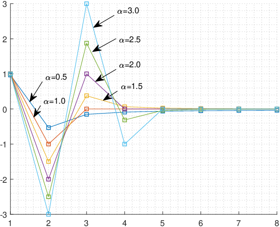
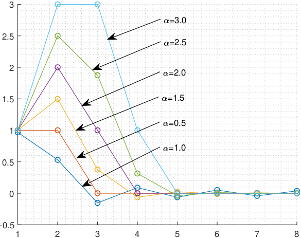
III-A Designing Filters
When takes an positive integer , if , the nonzero entries of and naturally have a distribution center, around at the th entry. In this case, what we need to do is to move the distribution center to the central position of and , around at th entry. If , according to (15) and (16), binomial expansion can not be fully placed in -dimension space, and superposition happens. In this case, usually there is no modulus distribution center in and . Of course, this phenomenon will happen when takes usual complex numbers. In all, the entries in and need to be rearranged in most cases.
In terms of the rule that entries closer to the filtering reference point should make more contributions to filtered consequence, the following steps are proposed for designing -dimensional hypercube filters and .
- step 1:
In -dimensional space, let be the filtering reference point;
- step 2:
- step 3:
According to the entry moduli, place the entries of and into the hypercube data block of and , the entries with larger moduli ought to be placed closer to the center of the block, .
Through step 1-3, and can be used for filtering. For a data sequence , whether its entries are real or complex numbers, usually the filtered consequence can reveal more details. The real/imaginary/angle/modulus information of the consequence has potential usefulness. Compared with and restricting to fractions [17], the imaginary and angle information is newly generated due to the nonzero imaginary part of . In practice, we can fuse all the information in terms of goals.
III-B Experimental Tests and Discussions
To show the performance of and , a large number of experimental tests have been done on all kinds of data.
III-B1 Filtering the synthetic data
In order to demonstrate the capability of to check changes with different frequencies, as well as the smooth capability of , we construct a synthetic data sequence as follows
which has three frequencies, and the components with higher frequency number have less amplitudes. We let and without any special aim, only for showing the relations between the primary data sequence and the components of the filtered result, and , as shown in Figure 2.


In Figure 2, comparing sub-figure (a) to (b) tells that, the imaginary part of , , looks quite similar to the result of the filter, LoG. Of course, the results other than the imaginary part, shown in sub-figure (b) and (c), are information not provided by LoG. The congruent relationships between and seem complex: 1) gets to the extremes about at the inflection points of , and 2) the phase angle of has big gap values at the inflection points where varies from concave to convex. Hence, integrating sub-figure (b) and (c) can tells more details of than the result due to LoG filter, which is only a fraction of . Comparing sub-figure (d) with (a), we can see and seem alike to the result due to the filter, Gaussian. In all, and uncover more secrets covered by than traditional filters designed in real domain, such as LoG and Gaussian filters.
III-B2 Filtering the benchmark visible-light image


Intensity images are 2-Dimensional signals, so without any lost of generalization, we use and to filter the image ‘Lena’11 1 https://www.ece.rice.edu/ wakin/images/, denoted as , which is very popular in image processing filed, somewhere of which has high frequency while someplace has low frequency.
First, we use a LoG filter with standard deviation and size to filter , the result is shown in Sub-figure (b) of Figure 3. The Filtered results of and are shown in Figure 4 and 5. Comparing Sub-figure (b) of Figure 3 with Figure 4, we can see that: 1) and and sub-figure (b) of Figure 3 are very like with each other, and the complementary image of (sub-figure (d) in Figure 4) shows the sketch of Lena; 2) , as shown in sub-figure (c) in Figure 4, has so many noises, and this result seems to demonstrate that is very sensitive to the changes in , even in the relative smooth areas there are so many noise points, and this phenomenon is consistent with that, phase correlation is very sensitive to noises. Comparing sub-figure (a), (b) and (c) with each other we can see they are different, and a bit complementary with each other. Comparing Figure 5 with Sub-figure (a) of Figure 3, we can see seems to enhance the area where relative larger changes happen; seems very like to , and too are and actually.


III-B3 Filtering TRUS (TRansrectal UltraSound) images


TRUS image is the main means for prostate cancer diagnosis and treatment,but this is always hampered by heavy speckles, as shown in subfigure (a) of Figure 6. How to find the diseased region and segment the prostate is rather challenging. Because there is no effective way to automatically complete the task, and it is still mainly performed by manual work up to now[19]. Due to heavy speckle noise, usually gradient operations do not be valid in disclosing the prostate boundary or in finding the diseased positions, though they behave admissibly for visible-light images. Using smooth filters to depress the speckles possibly benefit the analysis of the images, however from sub-figure (b) of Figure 6 as well as sub-figure (a), (b) and (d) of Figure 7, we can see the smoothed results still have heavy speckles, and do not highlight any image features which make the diseased area and boundary prominent. So, Gaussian smoothing, , as well as seem useless to identify the region of interest for TRUS images.


However, , shown in sub-figure (c) of Figure 7, seems very beneficial for indicating the diseased or boundary region. From sub-figure (c) of Figure 7, we can see that within the skeptical diseased regions there are so many extreme points of phase angles. Actually, in the region the prostate boundary is not clear, and it is in high probability that in the region tumour exists. Though , cannot indicate this even a little, but obviously show this. It seems very amazing, using this may provide significant improvement in handling TRUS images. A large number of tests was additionally done, and the found phenomenon seems robust, for example, the result shown in Figure 8, where sub-figure (b) also indicates the skeptical region. In all, complex-order filters seem very potential in handling images with heavy speckles.


III-B4 Discussions
In all above tests, takes , and the results, especially the ones on TRUS images, behave great potentially and promisingly. Of course, how to evaluate is vital for a real application. This problem is important, but up to now, there is no way to determine the appropriate calculus order for a real problem. So this problem is not discussed here. When takes complex number, and usually are complex numbers. Compared with the real , which makes and to be real numbers according to Theorem 1, complex makes and be complex numbers, and the real and imaginary parts, phase angle and modulus can be used to study . In some scenarios, phase angle behave amazingly compared with real and imaginary parts, as shown in sub-figure (b) of Figure 8 and sub-figure (c) of Figure 5. We can think, appropriately fusing real and imaginary parts may produce more meaningful apparatuses in practice.
IV Conclusions
In this paper, the filters with complex derivative or integral order are proposed. By multi-section trick, the complex-order filter has been proved to be the superposition of segments, gotten by partitioning the expansion sequence of the complex-order binomial. Compared with real number order filters, the complex order ones can uncover more information hidden in data sequence. A large number of tests have shown that the filters behave potentially and promisingly in disclosing features of data. Especially for the challenging problem of transrectal ultrasound images, the complex-order filters can indicate the diseased regions, and this cannot be done usually for real-order filters. In all, it is very hopeful that the complex-order filters will significantly benefit image processing and the associated fields
Acknowledgment
This work is supported by NSFC under grants 61860206007 and U19A2071.
References
- [1] Y.-F. Pu, P. Siarry, A. Chatterjee, Z.-N. Wang, Z. Yi, Y.-G. Liu, J.-L. Zhou, and Y. Wang, “A fractional-order variational framework for retinex: Fractional-order partial differential equation-based formulation for multi-scale nonlocal contrast enhancement with texture preserving,” IEEE Transactions on Image Processing, vol. 27, pp. 1214–1229, July 2018.
- [2] T. Levi-Civita, “The absolute differental at calculus (calculus of tensors),” Nature, vol. 120, pp. 542–543, Oct. 1927.
- [3] A. Fauth and C. A. Tudor, “Multifractal random walks with fractional brownian motion via malliavin calculus,” IEEE Transactions on Information Theory, vol. 60, no. 3, pp. 1963–1975, 2014.
- [4] H. Akçay, “Synthesis of complete orthonormal fractional basis functions with prescribed poles,” IEEE Transactions on Signal Processing, vol. 56, pp. 4716–4728, Oct. 2008.
- [5] Q. Zhou, J. Gao, Z. Wang, and K. Li, “Adaptive variable time fractional anisotropic diffusion filtering for seismic data noise attenuation,” IEEE Transactions on Geoscience and Remote Sensing, vol. 54, pp. 1905–1917, Apr. 2016.
- [6] M. Unser and N. Chenouard, “A unifying parametric framework for 2d steerable wavelet transforms,” SIAM J. IMAGING SCIENCES, vol. 6, no. 1, pp. 102–135, 2013.
- [7] J. L. Lovoie, T. J. Osler, and R. Tremblay, “Fractional derivatives and special functions,” SIAM Review, vol. 18, no. 2, pp. 240–268, 1976.
- [8] L. M. B. C. CAMPOS, “A review of definitions of fractional derivatives and other operators,” Journal of Computational Physics, vol. 388, pp. 195–208, July 2019.
- [9] X. Wei, D.-Y. Liu, , and D. Boutat, “Nonasymptotic pseudo-state estimation for a class of fractional order linear systems,” IEEE Transactions on Automatic Control, vol. 62, pp. 1150–1164, Mar. 2017.
- [10] A. I. Zayed, “A class of fractional integral transforms: A generalization of the fractional fourier transform,” IEEE Transactions on Signal Processing, vol. 50, pp. 619–627, Mar. 2002.
- [11] G. Jumarie, “An approach to differential geometry of fractional order via modified riemann¨cliouville derivative,” Acta Mathematica Sinica, English Series, vol. 28, p. 1741¨C1768, Sep. 2012.
- [12] D. Brockmann, L. Hufnagel, and T. Geisel, “The scaling laws of human travel,” Nature, vol. 439, pp. 462–465, Jan. 2006.
- [13] M. Breakspear, “Dynamic models of large-scale brain activity,” Nature Neuroscience, vol. 20, pp. 340¨C–352, Feb. 2017.
- [14] T. M. Atanacković, S. Konjik, S. Pilipović, and D. Zorica, “Complex order fractional derivatives in viscoelasticity,” Mechanics of Time-Dependent Materials, vol. 20, pp. 175–195, Jun 2016.
- [15] R. Andriambololona, “Real and complex order integrals and derivatives operators over the set of causal functions,” https://arxiv.org/abs/1302.4711.
- [16] L. M. B. C. CAMPOS, “On a concept of derivative of complex order with applications to special functions,” IMA Journal of Applied Mathematics, vol. 33, no. 2, pp. 109–133, 1984.
- [17] S. Das, ed., Functional Fractional Calculus. Berlin Heidelberg: Springer-Verlag, 2011.
- [18] K. R. Stromberg, Introduction to classical real analysis. Wadsworth International Group, 1981.
- [19] P. Wu, Y. Liu, Y. Li, and B. Liu, “Robust prostate segmentation using intrinsic properties of trus images,” IEEE Transactions on Medical Imaging, vol. 34, pp. 1321–1335, June 2015.