Kink-antikink collision in a Lorentz-violating modelJournal: Journal of LaTeX Templates
Abstract
In this work, kink-antikink collision in a two-dimensional Lorentz-violating model is considered. It is shown that the Lorentz-violating term in the proposed model does not affect the structure of the linear perturbation spectrum of the standard model, and thus there exists only one vibrational mode. The Lorentz-violating term impacts, however, the frequency and spatial wave function of the vibrational mode. As a consequence, the well-known results on kink-antikink collision will also change. Collisions of kink-antikink pairs with different values of initial velocities and Lorentz-violating parameters are simulated using the Fourier spectral method. Our results indicate that models with larger Lorentz-violating parameters would have smaller critical velocities and smaller widths of bounce windows. Interesting fractal structures existing in the curves of maximal energy densities of the scalar field are also found.
Keywords:
Kink collision, Lorentz-violating models , spectral methods1 Introduction
The domain wall is a simple type of topological soliton that exists in many nonlinear scalar field models. It plays an important role in many branches of physics. For instance, the duality between the sine-Gordon model and massive Thirring model provides the simplest example of bosonization in condensed-matter physics [1]. Cosmic domain walls can exist if the Universe was proceeded by some first-order phase transitions [2, 3]. It is even proposed that all of us might live on a four-dimensional domain wall embedded in a five-dimensional space-time [4, 5, 6, 7, 8, 9]; also see [10, 11] for reviews. A domain wall in dimensions is also called a kink.
The collision between non-integrable kinks is an important topic in the study of kinks. For the simplest kink-antikink collision, it is convenient to take the velocities of the kink and antikink as and , respectively. Such collisions are referred to as velocity-symmetric collisions or symmetric collisions in this paper. All the kink-antikink collisions mentioned below are of this type, only the velocity of the kink will be specified.
In integrable models, e.g., the sine-Gordon model, a kink and an antikink simply pass through each other after the collision, while in non-integrable models, however, the outcome of a kink-antikink collision sensitively depends on the initial velocity of the kink . Taking the model as an example, if is larger than the critical velocity , one observes inelastic scatterings with the emission of scalar radiation [12]. If , one usually observes a spatially localized oscillating structure called a bion or oscillon, which is a bound state of the kink and antikink [13]. However, if lies in some narrow intervals below , one would observe the interesting -bounce phenomenon; that is, after colliding times, kinks escape rather than trapping into a bion [14, 15]. These magical intervals are called -bounce windows (BWs), and have been found in many non-integrable models [16, 17]. More interestingly, all the -bounce windows form a fractal structure, which means that one may find some -bounce windows by zooming into the boundaries of an -bounce window [18].
According to the widely accepted Campbell-Schonfeld-Wingate (CSW) mechanism [15], the bounce-window phenomenon is caused by a resonant energy exchange between the vibrational mode and zero mode around a kink (antikink). However, some recent works reveal that the CSW mechanism is insufficient to describe bounce phenomena found in some non-integrable models in which the kink either has no vibrational mode at all [19], or only has quasinormal modes [20]. Therefore, by exploring kink-antikink collisions in various kinds of models one may find new phenomena with new physics.
Beyond the model, there are many works discussing kink-antikink collisions in models with both polynomial potentials [21, 22, 23, 24, 25, 26, 27, 28, 29, 30, 31, 32, 33] and triangular potentials [34, 35, 36, 37, 38], with noncanonical dynamics [39, 40], and with multiple scalar components [41, 42, 43, 44, 45]. In addition, multi-kink collisions have also been extensively studied recently [46, 47, 48, 49]. All these works assume Lorentz invariance of their models.
However, as pointed out in Ref. [50], every current candidate for a superunified theory11 1 A “superunified theory” is one which includes all known physical phenomena, and is valid up to Planck’s energy. contains some potentials for Lorentz violation, and the same is true for more restricted theories that attempt to treat quantum gravity alone. Theories with the potential for Lorentz violation, including superstring/M/brane theories, canonical and loop quantum gravity, non-commutative spacetime geometry, non-trivial space-time topology, and so on; see [51, 52, 53, 54, 55, 56] for part of the original works, and [57, 58, 59, 60, 61, 62] for recent reviews. Thus, it is interesting to search for kink solutions in Lorentz-violating scalar field theories, and study how Lorentz violation impacts the properties of the kinks and their collision.
Analytical static and traveling kink solutions have been found in some Lorentz-violating scalar field models with single or multi-field components [63, 64, 65, 66], and these solutions have been applied in many related issues, e.g., entropic information [67], the Kondo effect [68], and trapping fermions [69].
In this paper, kink-antikink interaction is considered by using the traveling kink solution reported in Ref. [63]. In the next section, the single-field Lorentz-violating model as well as the corresponding kink solution is reviewed. After an analysis of the linear stability, a numerical simulation of the kink-antikink collision is conducted.
2 Model and solution
The -dimensional Lorentz-violating scalar field model of [63] takes the following Lagrangian density:
| (1) |
with and The equation of motion reads
| (2) |
with . The violation of Lorentz symmetry is described by the parameter , which is assumed to be non-negative, , in this paper22 2 The model with can be obtained by applying the time-reversal transformation. Although the theory is not time symmetric and the behaviors are different from the case with , the same results are obtained when the space is reversed at the same time, because PT is conserved..
Obviously, the Lorentz-violating term does not alter the form of a static solution. Therefore, it is trivial to find a static kink solution. For example, a standard static kink solution
| (3) |
is obtained by taking the potential as
| (4) |
The real challenge is to find a traveling kink solution. The breaking of Lorentz invariance makes it difficult, in general, to find a boost transformation that helps derive traveling solutions from static ones. Fortunately, as mentioned in Ref. [63], the present model is invariant under a deformed boost transformation , where the deformed Lorentz factor is given by in the natural units33 3 The model is also translation invariant, so it possesses a deformed Poincaré symmetry.. Therefore, the traveling kink and antikink solutions take the following forms:
| (5) | |||||
| (6) |
where and are the initial position and velocity of the kink/antikink, respectively. A positive (negative) means a kink/antikink moving to the right (left). With the definition of , the allowed range of initial velocity varies with the value of the parameter :
| (7) |
which is shown in Fig. 1.

The energy density for a traveling solution is [63]
| (8) |
Obviously, in the Lorentz-violating model, the width and energy density of a moving kink depend on both the magnitude and direction of its velocity because of breaking of time symmetry. To see this phenomenon clearly, consider the linear superposition of a pair of a moving kink and antikink:
| (9) |
In Fig. 2, the configuration of and its energy density at time is plotted for . The asymmetry between the right-moving kink and left-moving antikink appears as increases. An antikink moving to the left has smaller width and larger energy density than those of a kink moving to the right with the same speed for . It is the opposite for .

3 Linear stability and vibrational mode
Before the discussion of kink-antikink collision, it is important to study the linear perturbation of the static kink solution. First, a good kink solution should be stable against the linear perturbation. In addition, according to the CSW mechanism, the existence of vibrational modes in a linear spectrum is closely connected with the bounce-window phenomenon.
To derive the equation of motion for a small perturbation vibrating around the static kink background , the action is expanded up to the second order of :
| (10) |
where with
| (11) |
After taking the variation of with respect to , the linear perturbation equation is obtained:
| (12) |
The following mode expansion is then introduced:
| (13) |
and substituted into Eq. (12) to obtain a Schrödinger-type equation for :
| (14) |
where . It is known from Eq. (2) that a static solution satisfies , which means , and Eq. (14) can be rewritten as
| (15) |
where (with ) is the Hamiltonian operator. It can be further factorized as [70, 71]
| (16) |
According to supersymmetric quantum mechanics, the eigenvalues of a system with a factorizable Hamiltonian are always non-negative, i.e., , which also means . Therefore, the static kink solution is stable against linear perturbation.
As can be seen from Eq. (14), the Lorentz-violating term does not affect the structure of the linear spectrum of the standard model. Thus, for the Lorentz-violating model considered here, there are two bound states: the translational mode (zero mode) and vibrational mode, and the corresponding eigenvalues and wave functions are [3]
| (17) | |||
| (18) |
However, one should note that the complete spatial wave function for the th mode is , which varies with , except for the zero mode; and . Therefore, the Lorentz-violating term does affect the shape of the vibrational mode, as shown in Fig. 3.
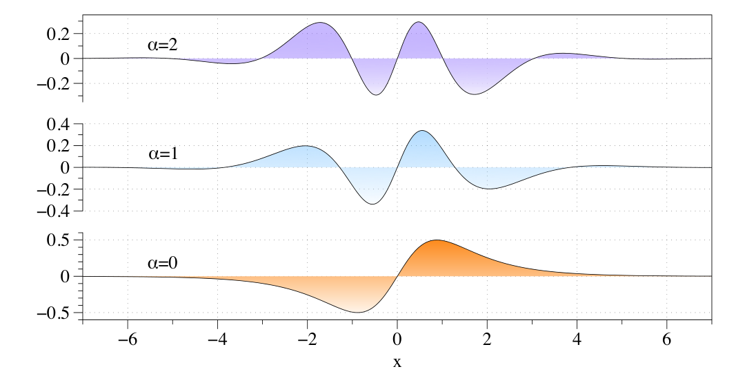
Since the vibrational mode is closely related to the bounce-window phenomenon, it is expected that the results of kink-antikink collision will also change with . This issue is discussed next.
4 Simulation and results
Unlike many integrable models, e.g., the sine-Gorden model, where analytical solutions for multiple kinks can be derived by using methods like Bäcklund transformation, it is extremely difficult to find multi-kink solutions in a non-integrable model. Therefore, to study the collision of a kink-antikink pair in the model proposed herein, one must resort to numerical simulation.
First, the initial condition of the system is taken as
| (19) |
where defined in Eq. (9) is a superposition of a kink initially at with velocity and an antikink initially at with velocity .
The dynamical equation (2) is solved by using the Fourier spectral method described in Refs. [72, 73, 40]. A reasonable numerical solution should satisfy the energy-conservation law, and this fact is used here to test the viability of the proposed numerical solution.
The total energy of the Lorentz-violating field is given by
| (20) |
For a well-separated kink-antikink pair, the total energy predicted by theory is
| (21) |
where is the energy of a soliton moving with speed , and is the total energy of the static soliton .
The conservation of the total energy is checked by evaluating the relative energy error:
| (22) |
Here, is the numerical result of the total energy, which is obtained by inserting the numerical solution of into Eq. (20). In this work, our simulations are implemented with a spatial grid step . The time step is automatically determined by the ode45 solver in MatLab (MathWorks, USA). The precision of the calculation can be controled by tuning or/and the tolerance options of the ode45 function, i.e., AbsTol and RelTol (see Ref. [40] for details). In our simulation, the tolerance options have been set to ensure that our numerical solutions of satisfy .
4.1 Impacts on fractal structure
To get a global idea of the influence of the Lorentz-violating term, first consider how the fractal structure would change under different values of . In Fig. 4, the fractal structures (up to three-bounce windows) are plotted for , and 1. The two-bounce windows (2BWs), three-bounce windows (3BWs), and the inelastic scattering zones are highlighted in green, pink, and gray, respectively. The un-highlighted zones correspond to higher-order bounce windows as well as bions. The critical velocity (the left-hand boundary of the gray zone) decreases from , to , and eventually to . As increases, all the 2BWs (the green zones) move to the left, and their widths decrease as well.
As an explicit example, the evolution of field configuration and the corresponding energy density for are plotted in Fig. 5. With this initial velocity, one would observe bion, two-bounce, and inelastic scattering by taking , and 1, respectively. From the bottom panels of Fig. 5, it can also be seen that the radiation emitted after collisions is asymmetric with respect to the origin.


The critical velocity for is plotted in Fig. 6, which shows that is a monotonically decreasing function of , and it is always below the maximum velocity allowed for a velocity-symmetric collision. Figure 7 shows how the widths of the first two 2BWs vary with respect to . It also decreases monotonically as becomes larger.
4.2 Information from maxima of energy densities
Given a value of , the fractal structure clearly shows how the collision results vary with the initial velocity . One may ask the reverse question; that is, given a value of , can one tell which interval of parameter corresponds to a two-bounce, three-bounce, or inelastic collision? In Ref. [49], the authors found that the maxima of various kinds of energy densities can provide important information on the collision phenomena. To see this, the energy density defined in Eq. (8) is first divided as follows:
| (23) |
where , , and are the kinetic energy density, elastic strain energy, and on-site potential energy, respectively (also see [74, 47]).
By simulating velocity-symmetric kink-antikink collisions with and , curves of the maxima of the aforementioned four types of energy densities are obtained: , and (see Fig. 8). These curves are qualitatively similar; that is, they show a fractal structure, i.e., in some intervals they behave in an orderly manner, but in several others they seem to be chaotic. The ordered intervals correspond to -bounce windows. The first three 2BWs, which correspond to , , and , are highlighted in green, and the first three 3BWs around the first 2BW, which correspond to , , and , in pink. In Fig. 9, the curves for the two- and three-bounce solutions are plotted, which correspond to some representative values of that lie in the highlighted bounce windows.
5 Summary
In this work, kink-antikink collisions of a Lorentz-violating model have been studied. After a short summary of the model and the kink solution of Ref. [63], the linear perturbation spectrum of the static kink solution was analyzed. It was found that the Lorentz-violating term of the proposed model does not change the spectrum structure of the standard model, so the static kink solution is linearly stable and there exists only one vibrational mode apart from a zero mode. However the Lorentz-violating term does impact the wave function and frequency of the vibrational mode. As a consequence, the kink-antikink collision phenomena of the present model will deviate from those of the standard model.
The deviation was studied numerically via two different approaches. In the first approach, fixing the values of the Lorentz-violating parameter to be , the collision with the initial velocity ranging from 0.12 to 0.27 was scanned. By comparing the fractal structures of each value of (Fig. 4), it was found that models with larger Lorentz-violating parameters have smaller critical velocities and narrower widths of 2BWs. The values of critical velocity and widths of 2BWs were also calculated for arbitrary values of (see Figs. 6 and 7).
In the second approach, setting the initial velocity as , the maximal energy densities corresponding to were scanned. An interesting fractal structure was observed for the first time (see Fig. 8). In the curves of maximal energy densities, the intervals corresponding to bions are more chaotic than those of the two bounces, three bounces, and inelastic scatterings. This indicates that the plot of maximal energy densities might be very useful in analyzing the results of kink collisions.
Phenomenological applications of the present work are worth consideration, but go beyond the scope of the present work.
Acknowledgements
Yuan Zhong thanks Zhi Xiao for discussions on Lorentz violation. This work was supported by the National Natural Science Foundation of China (Grant Nos. 11847211, 11605127 and 11875151), Fundamental Research Funds for the Central Universities (Grant No. xzy012019052), and China Postdoctoral Science Foundation (Grant No. 2016M592770). It was also supported in part by JSPS KAKENHI Grant Nos. JP17H06359 and JP19K03857, and by Waseda University Grant for Special Research Projects (Project Nos. 2019C-254 and 2020C-270).
Bibliography
References
- [1] S. Coleman, Aspects of symmetry: selected Erice Lectures of Sidney Coleman, Cambridge University Press, 1985.
- [2] A. Vilenkin, E. P. S. Shellard, Cosmic Strings and Other Topological Defects, Cambridge University Press, 2000.
- [3] T. Vachaspati, Kinks And Domain Walls, Cambridge University Press, 2006.
- [4] V. A. Rubakov, M. E. Shaposhnikov, Do we live inside a domain wall?, Phys. Lett. B 125 (1983) 136–138.
- [5] K. Akama, An Early Proposal of ’Brane World’, Lect.Notes Phys. 176 (1982) 267–271. arXiv:hep-th/0001113.
- [6] N. Arkani-Hamed, S. Dimopoulos, G. Dvali, The Hierarchy problem and new dimensions at a millimeter, Phys. Lett. B 429 (1998) 263–272. arXiv:hep-ph/9803315, doi:10.1016/S0370-2693(98)00466-3.
- [7] L. Randall, R. Sundrum, An alternative to compactification, Phys. Rev. Lett. 83 (1999) 4690–4693. arXiv:hep-th/9906064, doi:10.1103/PhysRevLett.83.4690.
- [8] L. Randall, R. Sundrum, A large mass hierarchy from a small extra dimension, Phys. Rev. Lett. 83 (1999) 3370–3373. arXiv:hep-ph/9905221, doi:10.1103/PhysRevLett.83.3370.
- [9] T. Shiromizu, K.-i. Maeda, M. Sasaki, The Einstein equation on the 3-brane world, Phys. Rev. D62 (2000) 024012. arXiv:gr-qc/9910076, doi:10.1103/PhysRevD.62.024012.
- [10] V. Dzhunushaliev, V. Folomeev, M. Minamitsuji, Thick brane solutions, Rept. Prog. Phys. 73 (2010) 066901. arXiv:0904.1775, doi:10.1088/0034-4885/73/6/066901.
- [11]
Y.-X. Liu,
Introduction
to Extra Dimensions and Thick Braneworlds (2018).
arXiv:1707.08541,
doi:10.1142/9789813237278_0008.
URL http://inspirehep.net/record/1611676/files/arXiv:1707.08541.pdf - [12] T. Sugiyama, Kink-antikink collisions in the two-dimensional model, Prog. Theor. Phys. 61 (1979) 1550–1563. doi:10.1143/PTP.61.1550.
- [13] A. E. Kudryavtsev, Solitonlike solutions for a higgs scalar field, JETP Lett. 22 (1975) 82.
- [14] M. Moshir, Soliton - Anti-soliton Scattering and Capture in Theory, Nucl. Phys. B 185 (1981) 318–332. doi:10.1016/0550-3213(81)90320-5.
- [15] D. K. Campbell, J. F. Schonfeld, C. A. Wingate, Resonance structure in kink-antikink interactions in theory, Physica D: Nonlinear Phenomena 9 (1983) 1. doi:10.1016/0167-2789(83)90289-0.
- [16] M. Peyrard, D. K. Campbell, Kink antikink interactions in a modified sine-gordon model, Physica D 9 (1983) 33–51.
- [17] D. K. Campbell, M. Peyrard, P. Sodano, Kink-antikink interactions in the double sine-Gordon equation, Physica D Nonlinear Phenomena 19 (1986) 165–205. doi:10.1016/0167-2789(86)90019-9.
- [18] P. Anninos, S. Oliveira, R. A. Matzner, Fractal structure in the scalar theory, Phys. Rev. D 44 (1991) 1147–1160. doi:10.1103/PhysRevD.44.1147.
- [19] P. Dorey, K. Mersh, T. Romanczukiewicz, Y. Shnir, Kink-antikink collisions in the model, Phys. Rev. Lett. 107 (2011) 091602. arXiv:1101.5951, doi:10.1103/PhysRevLett.107.091602.
- [20] P. Dorey, T. Romašœczukiewicz, Resonant kink-antikink scattering through quasinormal modes, Phys. Lett. B 779 (2018) 117–123. arXiv:1712.10235, doi:10.1016/j.physletb.2018.02.003.
- [21] V. A. Gani, A. E. Kudryavtsev, M. A. Lizunova, Kink interactions in the (1+1)-dimensional model, Phys. Rev. D 89 (2014) 125009. arXiv:1402.5903, doi:10.1103/PhysRevD.89.125009.
- [22] V. A. Gani, V. Lensky, M. A. Lizunova, Kink excitation spectra in the (1+1)-dimensional model, J. High Energy Phys. 08 (2015) 147. arXiv:1506.02313, doi:10.1007/JHEP08(2015)147.
- [23] E. Belendryasova, V. A. Gani, Scattering of the kinks with power-law asymptotics, Commun. Nonlinear Sci. Numer. Simulat. 67 (2019) 414. arXiv:1708.00403, doi:10.1016/j.cnsns.2018.07.030.
- [24] I. C. Christov, R. J. Decker, A. Demirkaya, V. A. Gani, P. G. Kevrekidis, A. Khare, A. Saxena, Kink-kink and kink-antikink interactions with long-range tails, Phys. Rev. Lett. 122 (17) (2019) 171601. arXiv:1811.07872, doi:10.1103/PhysRevLett.122.171601.
- [25] I. C. Christov, R. J. Decker, A. Demirkaya, V. A. Gani, P. G. Kevrekidis, R. V. Radomskiy, Long-range interactions of kinks, Phys. Rev. D 99 (1) (2019) 016010. arXiv:1810.03590, doi:10.1103/PhysRevD.99.016010.
- [26] A. R. Gomes, F. C. Simas, K. Z. Nobrega, P. P. Avelino, False vacuum decay in kink scattering, J. High Energy Phys. 10 (2018) 192. arXiv:1805.00991, doi:10.1007/JHEP10(2018)192.
- [27] T. S. Mendonca, H. P. de Oliveira, The collision of two-kinks defects, J. High Energy Phys. 09 (2015) 120. arXiv:1502.03870, doi:10.1007/J.HighEnergyPhys.09(2015)120.
- [28] T. S. Mendonca, H. P. de Oliveira, A note about a new class of two-kinks, J. High Energy Phys. 06 (2015) 133. arXiv:1504.07315, doi:10.1007/J.HighEnergyPhys.06(2015)133.
- [29] T. S. Mendonca, H. P. De Oliveira, The collision of two-kinks revisited: the creation of kinks and lump-like defects as metastable states, Braz. J. Phys. 49 (6) (2019) 914–922. arXiv:1808.04210, doi:10.1007/s13538-019-00703-3.
- [30] C. Adam, K. Oles, T. Romanczukiewicz, A. Wereszczynski, Kink-antikink scattering in the model without static intersoliton forces (2019). arXiv:1909.06901.
- [31] C. Adam, K. Oles, T. Romanczukiewicz, A. Wereszczynski, Spectral Walls in Soliton Collisions, Phys. Rev. Lett. 122 (24) (2019) 241601. arXiv:1903.12100, doi:10.1103/PhysRevLett.122.241601.
- [32] C. Adam, K. Oles, T. Romanczukiewicz, A. Wereszczynski, Thick spectral walls in solitonic collisions (12 2019). arXiv:1912.09371.
- [33] I. C. Christov, R. J. Decker, A. Demirkaya, V. A. Gani, P. Kevrekidis, A. Saxena, Kink-Antikink Collisions and Multi-Bounce Resonance Windows in Higher-Order Field TheoriesarXiv:2005.00154.
- [34] V. A. Gani, A. E. Kudryavtsev, Kink-antikink interactions in the double sine-Gordon equation and the problem of resonance frequencies, Phys. Rev. E 60 (1999) 3305–3309. arXiv:cond-mat/9809015, doi:10.1103/PhysRevE.60.3305.
- [35] V. A. Gani, A. M. Marjaneh, A. Askari, E. Belendryasova, D. Saadatmand, Scattering of the double sine-Gordon kinks, Eur. Phys. J. C 78 (4) (2018) 345. arXiv:1711.01918, doi:10.1140/epjc/s10052-018-5813-1.
- [36] D. Bazeia, E. Belendryasova, V. A. Gani, Scattering of kinks of the sinh-deformed model, Eur. Phys. J. C 78 (4) (2018) 340. arXiv:1710.04993, doi:10.1140/epjc/s10052-018-5815-z.
- [37] D. Bazeia, A. R. Gomes, K. Z. Nobrega, F. C. Simas, Kink scattering in hyperbolic models, Int. J. Mod. Phys. A 34 (2019) 1950200. arXiv:1902.04041, doi:10.1142/S0217751X19502002.
- [38] D. Bazeia, A. R. Gomes, K. Z. Nobrega, F. C. Simas, Kink scattering in a hybrid model, Phys. Lett. B 793 (2019) 26–32. arXiv:1805.07017, doi:10.1016/j.physletb.2019.04.013.
- [39] A. R. Gomes, R. Menezes, K. Z. Nobrega, F. C. Simas, Kink-antikink collisions for twin models, Phys. Rev. D 90 (6) (2014) 065022. arXiv:1312.7519, doi:10.1103/PhysRevD.90.065022.
- [40] Y. Zhong, X.-L. Du, Z.-C. Jiang, Y.-X. Liu, Y.-Q. Wang, Collision of two kinks with inner structure, J. High Energy Phys. 02 (2020) 153. arXiv:1906.02920.
- [41] A. Alonso-Izquierdo, Reflection, transmutation, annihilation and resonance in two-component kink collisions, Phys. Rev. D 97 (4) (2018) 045016. arXiv:1711.10034, doi:10.1103/PhysRevD.97.045016.
- [42] A. Alonso-Izquierdo, Kink dynamics in a system of two coupled scalar fields in two spacešCtime dimensions, Physica D 365 (2018) 12–26. arXiv:1711.08784, doi:10.1016/j.physd.2017.10.006.
- [43] A. Alonso-Izquierdo, A. J. Balseyro Sebastian, M. A. Gonzalez Leon, Domain walls in a non-linear -sigma model with homogeneous quartic polynomial potential, J. High Energy Phys. 11 (2018) 023. arXiv:1806.11458, doi:10.1007/JHEP11(2018)023.
- [44] A. Alonso-Izquierdo, Asymmetric kink scattering in a two-component scalar field theory model, Commun. Nonlinear Sci. Numer. Simul. 75 (2019) 200–219. arXiv:1901.03089, doi:10.1016/j.cnsns.2019.04.001.
- [45] A. Alonso-Izquierdo, Kink dynamics in the MSTB model, Phys. Scripta 94 (8) (2019) 085302. arXiv:1804.05605, doi:10.1088/1402-4896/ab1184.
- [46] A. M. Marjaneh, V. A. Gani, D. Saadatmand, S. V. Dmitriev, K. Javidan, Multi-kink collisions in the model, J. High Energy Phys. 07 (2017) 028. arXiv:1704.08353, doi:10.1007/JHEP07(2017)028.
- [47] A. M. Marjaneh, D. Saadatmand, K. Zhou, S. V. Dmitriev, M. E. Zomorrodian, High energy density in the collision of kinks in the model, Commun. Nonlinear Sci. Numer. Simul. 49 (2017) 30. arXiv:1605.09767, doi:10.1016/j.cnsns.2017.01.022.
- [48] A. M. Marjaneh, A. Askari, D. Saadatmand, S. V. Dmitriev, Extreme values of elastic strain and energy in sine-Gordon multi-kink collisions, Eur. Phys. J. B 91 (1) (2018) 22. arXiv:1710.10159, doi:10.1140/epjb/e2017-80406-y.
- [49] V. A. Gani, A. M. Marjaneh, D. Saadatmand, Multi-kink scattering in the double sine-Gordon model, Eur. Phys. J. C 79 (7) (2019) 620. arXiv:1901.07966, doi:10.1140/epjc/s10052-019-7125-5.
- [50] R. E. Allen, S. Yokoo, Searching for Lorentz Violation, Nuclear Physics B Proceedings Supplements 134 (2004) 139–146. arXiv:hep-th/0402154, doi:10.1016/j.nuclphysbps.2004.08.023.
- [51] S. M. Carroll, G. B. Field, R. Jackiw, Limits on a Lorentz- and parity-violating modification of electrodynamics, Phys. Rev. D 41 (4) (1990) 1231–1240. doi:10.1103/PhysRevD.41.1231.
- [52] S. M. Carroll, J. A. Harvey, V. A. Kostelecký, C. D. Lane, T. Okamoto, Noncommutative Field Theory and Lorentz Violation, Phys. Rev. Lett. 87 (14) (2001) 141601. arXiv:hep-th/0105082, doi:10.1103/PhysRevLett.87.141601.
- [53] V. A. Kostelecký, R. Lehnert, Stability, causality, and Lorentz and CPT violation, Phys. Rev. D 63 (6) (2001) 065008. arXiv:hep-th/0012060, doi:10.1103/PhysRevD.63.065008.
- [54] M. S. Berger, V. A. Kostelecký, Supersymmetry and Lorentz violation, Phys. Rev. D 65 (9) (2002) 091701. arXiv:hep-th/0112243, doi:10.1103/PhysRevD.65.091701.
- [55] V. A. Kostelecký, M. Mewes, Signals for Lorentz violation in electrodynamics, Phys. Rev. D 66 (5) (2002) 056005. arXiv:hep-ph/0205211, doi:10.1103/PhysRevD.66.056005.
- [56] Z. Xiao, B.-Q. Ma, Constraints on Lorentz invariance violation from gamma-ray burst GRB090510, Phys. Rev. D 80 (2009) 116005. arXiv:0909.4927, doi:10.1103/PhysRevD.80.116005.
- [57] D. Mattingly, Modern tests of Lorentz invariance, Living Rev. Rel. 8 (2005) 5. arXiv:gr-qc/0502097, doi:10.12942/lrr-2005-5.
- [58] Z. Xiao, B.-Q. Ma, Lorentz violation dispersion relation and its application, Int. J. Mod. Phys. A 24 (2009) 1359–1381. arXiv:0805.2012, doi:10.1142/S0217751X09042955.
- [59] W. Bietenholz, Cosmic Rays and the Search for a Lorentz Invariance Violation, Phys. Rept. 505 (2011) 145–185. arXiv:0806.3713, doi:10.1016/j.physrep.2011.04.002.
- [60] S. Liberati, Tests of Lorentz invariance: a 2013 update, Class. Quant. Grav. 30 (2013) 133001. arXiv:1304.5795, doi:10.1088/0264-9381/30/13/133001.
- [61] V. Kostelecky, N. Russell, Data Tables for Lorentz and CPT Violation, Rev. Mod. Phys. 83 (2011) 11–31. arXiv:0801.0287, doi:10.1103/RevModPhys.83.11.
- [62] M. D. C. Torri, Neutrino Oscillations and Lorentz Invariance Violation, Universe 6 (3) (2020) 37. doi:10.3390/universe6030037.
- [63] D. Bazeia, R. Menezes, Defect structures in Lorentz and CPT violating scenarios, Phys. Rev. D 73 (2006) 065015. arXiv:hep-th/0506262, doi:10.1103/PhysRevD.73.065015.
- [64] D. Bazeia, M. M. Ferreira, A. R. Gomes, R. Menezes, Lorentz-violating effects on topological defects generated by two real scalar fields, Physica D 239 (2010) 942–947. arXiv:1001.5286, doi:10.1016/j.physd.2010.01.015.
- [65] A. d. Souza Dutra, R. A. C. Correa, Traveling solitons in Lorentz and CPT breaking systems, Phys. Rev. D 83 (2011) 105007. arXiv:1012.0268, doi:10.1103/PhysRevD.83.105007.
- [66] E. Passos, C. A. G. Almeida, F. A. Brito, R. Menezes, J. C. Mota-Silva, J. R. L. Santos, Soliton solutions in two-dimensional Lorentz-violating higher derivative scalar theory, Annals Phys. 396 (2018) 351–370. arXiv:1610.04216, doi:10.1016/j.aop.2018.07.025.
- [67] R. A. C. Correa, R. a. da Rocha, A. de Souza Dutra, Entropic information for travelling solitons in Lorentz and CPT breaking systems, Annals Phys. 359 (2015) 198–212. arXiv:1501.02000, doi:10.1016/j.aop.2015.04.027.
- [68] D. Bazeia, F. A. Brito, J. C. Mota-Silva, Kondo effect from a Lorentz-violating domain wall description of superconductivity, Phys. Lett. B 762 (2016) 327–333. arXiv:1606.07051, doi:10.1016/j.physletb.2016.09.043.
- [69] R. A. C. Correa, W. de Paula, A. de Souza Dutra, T. Frederico, Lorentz Violation and Topologically Trapped Fermions in 2+1 Dimensions, Annalen Phys. 530 (5) (2018) 1700405. arXiv:1703.10591, doi:10.1002/andp.201700405.
- [70] Y. Zhong, R.-Z. Guo, C.-E. Fu, Y.-X. Liu, Kinks in higher derivative scalar field theory, Phys. Lett. B 782 (2018) 346. arXiv:1804.02611, doi:10.1016/j.physletb.2018.05.048.
- [71] Y. Zhong, Y.-X. Liu, -field kinks: stability, exact solutions and new features, J. High Energy Phys. 1410 (2014) 41. arXiv:1408.4511, doi:10.1007/J.HighEnergyPhys.10(2014)041.
- [72] L. N. Trefethen, Spectral Methods in Matlab, Society for Industrial and Applied Mathematics, Philadelphia, PA, 2000.
- [73] Y.-Q. Wang, Y.-X. Liu, R.-G. Cai, S. Takeuchi, H.-Q. Zhang, Holographic SIS Josephson Junction, J. High Energy Phys. 09 (2012) 058. arXiv:1205.4406, doi:10.1007/JHEP09(2012)058.
- [74] D. Saadatmand, S. V. Dmitriev, P. G. Kevrekidis, High energy density in multisoliton collisions, Phys. Rev. D 92 (5) (2015) 056005. arXiv:1506.01389, doi:10.1103/PhysRevD.92.056005.
- [75]
A. Askari, D. Saadatmand, S. V. Dmitriev, K. Javidan,
High
energy density spots and production of kinkšcantikink pairs in particle
collisions, Wave Motion 78 (2018) 54 – 59.
doi:https://doi.org/10.1016/j.wavemoti.2018.01.003.
URL http://www.sciencedirect.com/science/article/pii/S0165212518300118