Interplay between superconductivity and non-Fermi liquid at a quantum-critical point in a metal.
I: The model and its phase diagram at . The case .
Abstract
Near a quantum-critical point in a metal a strong fermion-fermion interaction, mediated by a soft boson, acts in two different directions: it destroys fermionic coherence and it gives rise to an attraction in one or more pairing channels. The two tendencies compete with each other. We analyze a class of quantum-critical models, in which momentum integration and the selection of a particular pairing symmetry can be done explicitly, and the competition between non-Fermi liquid and pairing can be analyzed within an effective model with dynamical electron-electron interaction (the -model). In this paper, the first in the series, we consider the case and . We argue that tendency to pairing is stronger, and the ground state is a superconductor. We argue, however, that a superconducting state is highly non-trivial as there exists a discrete set of topologically distinct solutions for the pairing gap (). All solutions have the same spatial pairing symmetry, but differ in the time domain: changes sign times as a function of Matsubara frequency . The solution is sign-preserving and tends to a finite value at , like in BCS theory. The solution corresponds to an infinitesimally small , which oscillates down to the lowest frequencies as , where and is of order of fermion-boson coupling. As a proof, we obtain the exact solution of the linearized gap equation at on the entire frequency axis for all , and an approximate solution of the non-linear gap equation. We argue that the presence of an infinite set of solutions opens up a new channel of gap fluctuations. We extend the analysis to the case where the pairing component of the interaction has additional factor and show that there exists a critical , above which superconductivity disappears, and the ground state becomes a non-Fermi liquid. We show that all solutions develop simultaneously once gets smaller than .
I Introduction.
The interplay between superconductivity and pairing near a quantum-critical point (QCP) in a metal is a fascinating subject, which attracted substantial attention in the correlated electron community after the discovery of superconductivity (SC) in the cuprates, heavy-fermion and organic materials, and, more recently, Fe-pnictides and Fe-chalcogenides. (see, e.g., Refs. Monthoux et al. 2007; Scalapino 2012; Norman 2014; Maiti and Chubukov 2014; Keimer et al. 2015; Shibauchi et al. 2014; Fernandes and Chubukov 2016; Fradkin et al. 2010; Yang et al. 2006; Fratino et al. 2016; Sachdev 2018; Coleman 2015). Itinerant QC models, analyzed analytically in recent years include, e.g., models of fermions in spatial dimensions (Refs. Mross et al. 2010; Metlitski et al. 2015; Mahajan et al. 2013; *raghu2; *raghu3; *raghu4; *raghu5; Wang et al. 2018; Wang et al. 2017a; Fitzpatrick et al. 2015b), two-dimensional (2D) models near a spin-density-wave (SDW) and charge-density-wave (CDW) instabilities (Refs. Millis 1992; Altshuler et al. 1995a; Sachdev et al. 1995; Abanov et al. 2001a; Abanov et al. 2003; *acs2; *finger_2001; *acn; Sachdev et al. 2009; *Subir2; *Sachdev2019; Vojta and Sachdev 1999; Wang and Chubukov 2013a; Efetov et al. 2013; *efetov2; *efetov3; Tsvelik 2017; Metlitski and Sachdev 2010a; Dalidovich and Lee 2013; *sslee_2018; Bauer and Sachdev 2015; Castellani et al. 1995; *ital2; *ital3; Wang and Chubukov 2013a; *wang23; *wang_22; Khodas et al. 2010; *tsvelik; *tsvelik_1; *tsvelik_2; *tsvelik_3; Metzner et al. 2003; *DellAnna2006; Vilardi et al. 2018; *metzner_1; *metzner_2; Sordi et al. 2012; Chubukov and Wölfle 2014), density-wave instability (Refs.Altshuler et al. 1995b; *2kf2; *2kf3), pair-density-wave instability Kim et al. 2008; Lawler and Fradkin 2007; *Fradkin2009; *Fradkin2014, instabilities towards a Pomeranchuk order instabilityBonesteel et al. 1996; *Oganesyan2001; *q=01; *q=02; Metzner et al. 2003; *DellAnna2006; Rech et al. 2006; Lee 2009; Metlitski and Sachdev 2010b; Lederer et al. 2015; Maslov and Chubukov 2012; *maslov2; *maslov3; *maslov4; You et al. 2016; Wang et al. 2001; *triplet2; *triplet3; Lederer et al. 2017; Klein et al. 2019; *avi_2 and towards circulating currents Bok et al. 2016, 2D fermions at a half-filled Landau level Lee 1989; *Monien1993; *Nayak1994; *Altshuler1994; *Kim_1994, generic QC models with different critical exponents Raghu et al. 2015; Moon and Chubukov 2010; Khveshchenko and Shively 2006; She and Zaanen 2009; *She2010; Wang et al. 2016; Lee et al. 2018; Wu et al. 2019a; Wu et al. 2019b; *Abanov_19; Yuzbashyan et al. a, Sachdev-Ye-Kitaev (SYK) and SYK-Yukawa models Patel and Sachdev 2019; Esterlis and Schmalian 2019; Wang 2020; Hauck et al. 2019; Chowdhury and Berg 2020, strong coupling limit of electron-phonon superconductivity, Combescot 1995; Bergmann and Rainer 1973; *Bergmann2; *ad; Marsiglio et al. 1988; *Marsiglio_91; Karakozov et al. 1991; Chubukov et al. 2020a, and even color superconductivity of quarks, mediated by gluon exchangeSon 1999; *son2. These problems have also been studied using various numerical techniques Yang et al. 2011; Gerlach et al. 2017; *berg_2; *berg_3; *berg_4; Haule and Kotliar 2007; *kotliar2; Sordi et al. 2012; Georges et al. 2013; *georges2.
From theory perspective, the key interest in the pairing near a QCP is due to the fact that an effective dynamic electron-electron interaction, , mediated by a critical collective boson, which condenses at a QCP, provides strong attraction in one or more pairing channels and, at the same time, gives rise to non-Fermi liquid (NFL) behavior in the normal state. The two tendencies compete with each other: fermionic incoherence, associated with NFL behavior, destroys Cooper logarithm and reduces the tendency to pairing, while the opening of a SC gap eliminates the scattering at low energies and reduces the tendency to NFL. To find the winner (SC or NFL), one needs to analyze the set of integral equations for the fermionic self-energy, , and the gap function, , for fermions with momentum/frequency and .
We consider the subset of models in which collective bosons are slow modes compared to dressed fermions, for one reason or the other. In this situation, which bears parallels with Eliashberg theory for electron-phonon interaction Eliashberg 1960, the self-energy and the pairing vertex can be approximated by their values at the Fermi surface (FS) and computed within one-loop approximation. The self-energy on the FS, is invariant under rotations from the point group of the underlying lattice. The rotational symmetry of the gap function and the relation between the phases of on different FS’s in multi-band systems are model specific. Near a ferromagnetic QCP, the pairing interaction mediated by a soft boson is attractive in the p-wave channel. Near an antiferromagnetic QCP, the strongest attraction is in wave channel for the case of a single FS and fermionic density near half-filling. For a nearly compensated metal with hole and electron pockets, as in Fe-based superconductors, the two attractive channels near an antiferromagnetic QCP are and wave. Near a nematic QCP, the pairing interaction, mediated by soft nematic fluctuations, is attractive in all channels: wave, wave, wave, etc. In each particular case, one has to project the pairing interaction into the proper irreducible channel, find the strongest one, and solve for the pairing vertex within a given pairing symmetry. In principle, even after projection, one has to solve an infinite set of coupled equations in momentum space as in a lattice system each irreducible representation contains an infinite set of eigenfunctions. However, near a QCP the pairing is often confined to a narrow range on the FS around special ”hot spots”. In this situation, the momentum integration near the FS can be carried out exactly, and the set of coupled equations for the self-energy and the gap function reduce to two one-dimensional (1D) equations for and , each with frequency-dependent effective ’local” interaction (Ref. Abanov et al. 2001a. The same holds for the cases of s-wave pairing by a soft optical phonon, when momentum-dependencies of and are not crucial and can be neglected, of non-s-wave pairing, when one eigenfunction gives the dominant contribution to the gap (e.g., for wave pairing in the cuprates), and for the case when the fermionic density of states is peaked at particular due to, e.g. van-Hove singularities ( see e.g., Maiti and Chubukov 2014 and references therein).
Away from a QCP, the effective tends to a finite value at . In this situation, the fermionic self-energy has a FL form at the smallest frequencies, the equation for is similar to that in a conventional Eliashberg theory for phonon-mediated superconductivity, and the only qualitative distinction for electronically-mediated pairing is that by itself changes below due to feedback from fermionic pairing on collective modes.
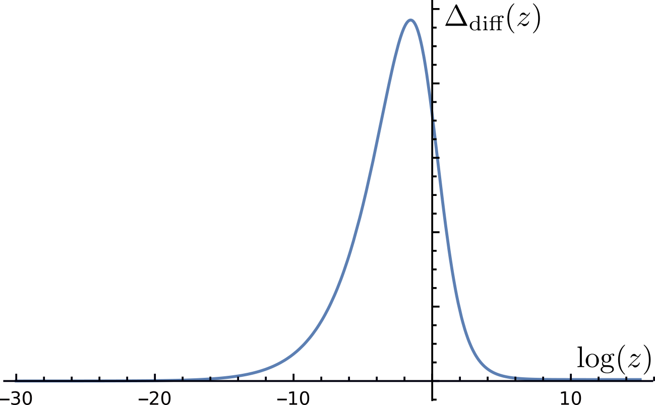
At a QCP, the situation becomes qualitatively different because the effective interaction , mediated by a critical massless boson, becomes a singular function of frequency: on Matsubara axis (Fig. 1). The exponent depends on the model, ranging from small in models in to in 2D models at SDW, CDW, and nematic QCP and in Yukawa-SYK model Chubukov et al. 2020b; Maiti and Chubukov 2014; Chubukov et al. 2020a; Esterlis and Schmalian 2019; Wang 2020. The case corresponds to fermions, interacting with a critical Einstein phonon. The set of models with has been nicknamed the -model, and we will use this notation. We present an (incomplete) set of models in Tables 1- 3.


In this and subsequent papers, we present comprehensive analysis of the competition between NFL and SC within the model. We define the dimensionless as , where is the effective fermion-boson coupling. This is the only parameter in the model with the dimension of energy, and we will see that it determines both the magnitude of the gap function and the upper limit of NFL behavior in the normal state, i.e., the scale below which . We show that the competition between NFL and SC holds for all values of , but the physics and the computational analysis are different for the models with , , , , and , which we consider separately. We show that for all , a NFL self-energy in the normal state does not prevent the formation of bound pairs of fermions at a non-zero onset temperature . However, we argue that is generally higher than the actual superconducting , and at bound pairs remain incoherent. In this range various observables, e.g., the spectral function and the density of states, display pseudogap behavior. This holds for all , but the width of the pseudogap phase increases with . We relate the pseudogap behavior to strong gap fluctuations, but argue that these fluctuations can be viewed as long-wavelength phase fluctuations only in some range . At smaller , pseudogap behavior is predominantly due to the existence of low-energy ’longitudinal” gap fluctuations, which change the functional form of and cause phase slips. We argue that longitudinal gap fluctuations develop a zero mode at in which case SC order gets destroyed already at . Specifically, the presence of a zero mode implies that there exists an infinite number of solutions for , all with the same condensation energy. In this situation, the ground state is a mixture of different , each with its own phase. We will argue that gradually vanishes at and remains zero at larger , while and stay finite. We show the phase diagram in Fig. 2. Our results present the scenario for the pseudogap, which holds even if for a given solution for SC stiffness is larger than , i.e., conventional phase fluctuations are weak. This scenario is complementary to the one in which the smallness of the superfluid stiffness is caused by the closeness to a Mott transition (see, e.g., Ref. Simard et al. 2019 and references therein).
I.1 A brief summary of the results of this work
In this paper, the first in the series, we analyze the -model at at . For definiteness we focus on spin-singlet pairing. The analysis of spin-triplet pairing is more involved because of different spin factors in the self-energy and the pairing vertex Wang et al. 2001; Roussev and Millis 2001; Chubukov et al. 2003 In this paper we discuss even frequency pairing. The analysis of odd-frequency pairing Linder and Balatsky 2019 is more involved and requires a separate consideration.
Our key goal is to understand the interplay between the competing tendencies toward pairing and toward NFL behavior. The first comes from the interaction in the particle-particle channel, the second from the interaction in the particle-hole channel. In the original -model, both interactions are given by the same . In order to separate the two tendencies we extend the model and introduce the knob to vary the relative strength of the interaction in the two channels. Specifically, we multiply the pairing interaction by and treat as a parameter. For () the tendency towards pairing decreases (increases) compared to the one towards NFL ground state. The extension to integer can be formally justified by extending the model from to an global symmetry Raghu et al. 2015. In our analysis, we use the extension to arbitrary just as a computational trick to better understand what happens in the physical case of .

The phase diagram of the -model for has been studied before Raghu et al. 2015; Wang et al. 2016. It was argued that for any there exists a critical , separating a SC ground state at and a normal, NFL ground state at (see Fig. 3). The physical case falls into the SC region. A similar result has been recently found in the study of the pairing in the SYK-type model Hauck et al. 2019.
The conventional wisdom holds that for , is infinitesimally small for , and has a finite value for , i.e., that the linearized gap equation has the solution at , and the non-linear gap equation has the solution for . We argue that in our case the conventional wisdom fails. Namely, we prove that the linearized equation has a solution not only for , but also for all , including the physical case of . We obtain the exact solution of the linearized gap equation, , for all and all . This oscillates at small as , where and are particular functions of (for a given ), e.g., for . At large , decreases as (see Fig. 11).
At small , when is a smooth function of frequency, the integral equation for can be approximated by second-order differential equation, whose solution, , also exists for all and can be expressed analytically as a combination of two complex-conjugated hypergeometric functions. This also oscillates at small and decays as at large frequencies (see Fig. 9). We show that coincides with the exact to leading order in .
We then analyze the non-linear gap equation. We argue that it has an infinite, discrete set of solutions, specified by integer , which ranges between and . All solutions have the same spatial gap symmetry (i.e., -wave, wave, etc). A solution changes sign times as a function of frequency. Each tends to a finite value at , but the magnitude of progressively decreases with increasing . At , is the solution of the linearized gap equation, which has an infinite number of sign changes due to oscillations running down to the smallest . The solution yields sign-preserving .
The existence of an infinite set of , each representing a local minimum of the Luttinger-Ward (LW) functional, opens up a new channel of longitudinal gap fluctuations, which cause phase slips. As long as the set is discrete, there is a single global minimum of the LW functional. In our case, it corresponds to . Then, at the system should display a SC order. Still, the existence of the infinite set of is a non-trivial aspect of the pairing at a QCP. In the next paper, we analyze the -model for at a finite and show explicitly that for any there exists a discrete, infinite set of onset temperatures for the pairing, , and the corresponding eigenfunctions change sign times as a function of Matsubara frequency. We argue that at , each approaches the solution of the non-linear integral gap equation at . We show that away from a QCP, only solutions with remain, where decreases with the deviation from a QCP.
We note in passing that a discrete set of solutions for the gap function at , with different momentum dependencies along the FS, has been detected in the analysis of near a nematic QCP, Refs. Yang and Sondhi 2000; Klein et al. 2019 There, however, the physics is different, and the number of solutions is finite at a QCP. This is similar to our case away from a critical point.

I.2 Relevance of the exact solution of the linearized gap equation
The existence of an infinite set of solutions of the non-linear gap equation is a direct consequence of a highly unusual result that at a QCP the linearized gap equation has a solution not only at , but also for any (see Fig. 4). This does not away from a QCP, where the linearized gap equation as a solution only at . The proof of the existence of the solution for infinitesimally small for all , including the original , is, therefore, the central element of our analysis.

The linearized gap equation can be analyzed at frequencies much smaller and much larger than . In these two limits one can truncate the gap equation by keeping only leading terms either in or in . The truncated equation can be solved and yields at large and at small , where the phase factor is a free parameter. The generic task is then to verify whether by fixing one can find , which smoothly interpolates between small and large (see Fig. 5). The verification would be straightforward if there was a finite frequency range where both forms were valid and could be made equal by fixing . In our case, however, the low-frequency and the high-frequency regimes do not overlap, so the only option is to solve the full equation. We present the exact solution and show that at small and large frequencies it reduces to known forms. The analytic expression for is rather complex, but one can straightforwardly plot for any input parameters (see Fig. 11).
At small , where the interaction is a slowly varying function of frequency, the actual, integral gap equation can be approximated by a differential equation. The latter can be solved analytically, and the solution, , is a hypergeometric function of . Using the properties of a hypergeometric function at small and large values of the argument one can explicitly verify that does interpolate between the known forms at small and large if one properly chooses the value of the phase .
We show that and coincide at small and use the analytic form of to analyze the structure of the gap function at different . We demonstrate by the direct comparison that at larger , and differ qualitatively. We argue that the series for the exact contain non-local terms, not present for . These non-local terms are negligible at small , but must be kept for , particularly near , which separates oscillating behavior at smaller and decay at larger .
I.3 Structure of the paper
The paper is organized as follows. In Sec. II we briefly review the -model and extend it to . We present the set of coupled Eliashberg equations for the pairing vertex and the fermionic self-energy and combine them into the equations for the gap function and the inverse quasiparticle residue .
In Secs. III and IV we study the linearized gap equation with infinitesimally small . In Sec. III we analyze the truncated gap equation at small and large and obtain the solutions, valid in the corresponding limits. Here we identify and show that the solution at small frequencies changes qualitatively between and . In Sec. IV we consider the limit of small and approximate the actual integral gap equation by second-order differential equation. We solve the differential equation for all and explicitly show how one can match low-frequency and high-frequency forms by fixing a single phase factor. We show that this only holds for , while for the potential solution does not satisfy the condition of normalizability. In Sec. V we obtain the exact solution of the full linearized gap equation. We show that it exists for all . The solution, , oscillates at small frequencies and decays as at large . In Sec. V.1 we analyze the structure of and compare it with . We show that the two coincide at the smallest , but differ at . We argue that the difference is due to the fact that contain non-local terms, not present in . In Sec. VI we consider the non-linear gap equation. We first analyze the non-linear differential equation and argue that it has an infinite, discrete set of solutions for any . The index specifies the number of times changes sign as a function of frequency. The solution with is sign-preserving. The solution coincides with the solution of the linearized differential equation. We conjecture that the actual, non-linear integral gap equation also possesses an infinite, discrete set of topologically distinct solutions . Sec. VII presents the summary of our results.
I.4 Brief outline of subsequent papers
In the next paper in the series (Paper II, Ref. Wu et al. 2020) we consider the linearized gap equation for the same range at a finite and show that there exists an infinite discrete set of critical temperatures for the pairing instability, all within the same pairing symmetry. The corresponding eigenfunction changes sign times as a function of discrete Matsubara frequency . We argue that at these finite solutions become , which we find here in the analysis.
For , the sign-preserving solution has the largest condensation energy and the largest . Still, the presence of an infinite set of at is not only highly unusual, but creates a new channel of ”longitudinal” gap fluctuations. In subsequent papers we will focus on the physical case and extend the analysis at to . We will show that the set becomes more dense with increasing and eventually becomes continuous at . For this special , all solutions of the non-linear gap equation with finite have equal condensation energy, and long-range superconducting order at gets destroyed upon averaging over these solutions, each with its own phase. We will corroborate this by the analysis of the gap equation for the same at finite and obtain the phase diagram, shown in Fig. 2. Later, we will show Yuzbashyan et al. b that the system behavior is rather special for larger , particularly for .
II -model.
We consider itinerant fermions at the onset of a long-range order in either spin or charge channel. At the critical point, the propagator of a soft boson becomes massless and mediates singular interaction between fermions. We follow earlier works Abanov et al. 2001a; Abanov et al. 2003; Moon and Chubukov 2010; Metlitski and Sachdev 2010b; Mross et al. 2010; Monthoux et al. 2007; Efetov et al. 2013; Metlitski et al. 2015; Raghu et al. 2015; Haslinger and Chubukov 2003; Wang et al. 2016; Lee et al. 2018 and assume that this interaction is attractive in at least one pairing channel and that a pairing boson can be treated as slow mode compared to a fermion, i.e., at a given momentum , typical fermionic frequency is much larger than typical bosonic frequency. This is the case for a conventional phonon-mediated superconductivity, where for a typical fermionic frequency is of order , while typical bosonic frequency is of order Debye frequency . The ratio is the small parameter for Eliashberg theory of phonon-mediated superconductivity. This theory allows one to obtain a set of coupled integral equations for frequency dependent fermionic self-energy and the pairing vertex. By analogy, the theory of electronic superconductivity, mediated by soft collective bosonic excitations in spin or charge channel, is also often called Eliashberg theory. We will use this convention.
Within the Eliashberg approximation, one can explicitly integrate over the momentum component perpendicular to the Fermi surface (for a given pairing symmetry) and reduce the pairing problem to a set of coupled integral equations for frequency dependent self-energy and the pairing vertex with effective frequency-dependent dimensionless interaction . This interaction gives rise to NFL form of the self-energy in the normal state and, simultaneously, gives rise to the pairing.
At , the coupled Eliashberg equations for the pairing vertex and the fermionic self-energy are, in Matsubara formalism,
| (1) |
where . In these equations, both and are real functions. Observe that we define with the overall plus sign and without the overall factor of . 11 1 In obtaining the Eliashberg equations we assumed that states away from the Fermi surface are irrelevant for the pairing and NFL behavior, and extended the integration over momenta to infinite limits. In this situation, fermionic self-energy is real. If the momentum integration over holds in finite and non-symmetric limits, has both real and imaginary components. The same holds in SYK-type models at a non-zero chemical potential (see Ref. Gu_2020 and references therein). In the normal state (),
| (2) |
where . At small , .
The superconducting gap function is defined as a real function
| (3) |
The equation for is readily obtained from (II):
| (4) |
This equation contains a single function , but for the cost that appears also in the r.h.s., which makes Eq. (4) less convenient for the analysis than Eqs. (II).
Eqs. (II)-(4) describe color superconductivity Son 1999; *son2 and pairing in 3D (, ), spin- and charge-mediated pairing in dimensions Mross et al. 2010; Metlitski et al. 2015; Raghu et al. 2015 and superconductivity in graphene Khveshchenko 2009 (), a 2D pairing Altshuler et al. 1995b with interaction peaked at (), pairing at a 2D nematic/Ising-ferromagnetic QCP Bonesteel et al. 1996; Lederer et al. 2015; Wang et al. 2001; *triplet2; *triplet3 (), pairing at a 2D SDW QCP Millis 1992; Abanov et al. 2001a; Abanov et al. 2003; Wang and Chubukov 2013a and an incommensurate CDW QCP Castellani et al. 1995; *ital2; *ital3; Chowdhury and Sachdev 2014b; *wang_22; *wang23 (), dispersionless fermions randomly interacting with an Einstein phonon Esterlis and Schmalian 2019; Wang 2020; Hauck et al. 2019 and a spin-liquid model for the cuprates Tsvelik 2017 () a 2D pairing mediated by an undamped propagating boson (), pairing in several Fe-based superconductors Haule and Kotliar 2007 () and even the strong coupling limit of phonon-mediated superconductivity for either dispersion-full Combescot 1995; Bergmann and Rainer 1973; *Bergmann2; *ad; Marsiglio et al. 1988; *Marsiglio_91; Karakozov et al. 1991 or dispersion-less Esterlis and Schmalian 2019; Wang 2020 fermions (). The pairing models with parameter-dependent have been analyzed as well (Refs. Sachdev et al. 2009; Moon and Chubukov 2010). The case describes a BCS superconductor. We list some of the model in Tables 1 - 3.
A justification of Eliashberg theory for electronically mediated superconductivity (e.g., the reasoning to neglect vertex corrections) is case specific. For Ising-nematic fluctuations (the case ), vertex corrections are small in , which is a small parameter of the theory Metzner et al. 2003; *DellAnna2006; Maslov and Chubukov 2010; Klein et al. 2020; *avi_last_1. In other cases, e,g., in SYK models, a small parameter for Eliashberg approximation is , where is the number of of fermionic flavors Patel and Sachdev 2019; Esterlis and Schmalian 2019; Wang 2020; Hauck et al. 2019; Chowdhury and Berg 2020. For several 2D models, the corrections to Eliashberg approximation for the self-energy in the normal state are logarithmically singular and in the absence of the pairing would change the system behavior at the smallest frequencies Abanov et al. 2003; Metlitski and Sachdev 2010a; Dalidovich and Lee 2013; *sslee_2018. One-loop logarithmic corrections just change but keep the model intact (Ref. Abanov et al. 2003), but higher-order corrections go beyond the model (Refs. Metlitski and Sachdev 2010a; Dalidovich and Lee 2013; *sslee_2018). Here, we assume that the onset temperature for the pairing, , is larger, at least numerically, than the scale at which corrections to Eliashberg approximation become relevant, and stick with the Eliashberg theory. Recent Quantum Monte Carlo (QMC) calculations for superconductivity, mediated by antiferromagnetic spin fluctuations Wang et al. 2017b and Ising-nematic fluctuations Klein et al. 2020, have found the onset of superconductivity at a temperature, almost identical to the one in the model with and , respectively, without vertex corrections. Normal state QMC calculations for the models with antiferromagnetic and Ising-nematic fluctuations also found Klein et al. 2020; *avi_last_1 very good agreement with the behavior of the models with and . A good agreement has been also found between QMC calculations of superconducting for electron-phonon interaction and the -model with (Ref. Chubukov et al. 2020a), for couplings smaller than the Fermi energy.
|
|
|
| |||||
|---|---|---|---|---|---|---|---|---|
|
|
|
| |||||
|
|
|
| |||||
|
|
|
| |||||
|
|
|
|
|
|
|
| ||||||
|
|
|
| ||||||
|
|
|
| ||||||
|
|
|
| ||||||
|
|
|
|
|
|
| |||||
|---|---|---|---|---|---|---|---|---|
|
|
|
| |||||
|
|
|
|
In this paper, we consider the set of -models with . The analysis for requires separate consideration because of divergencies in the r.h.s. of both equations in (II) (but not in (4)) and will be presented in subsequent papers.
Notice that for any the pairing interaction decays at large frequencies as . A simple experimentation shows that the integrals in (II) and (4) are then convergent in the ultraviolet. The only exceptions are the BCS case , when is just a constant, and the case , i.e., (color superconductivity/pairing in 3D, Refs. Son 1999; *son2; Metlitski et al. 2015). For these two cases one needs to set the upper cutoff of frequency integration at some to cut ultra-violet divergence. We discuss the limit in Appendix A.
The full set of Eliashberg equations for electron-mediated pairing contains also the equation describing the feedback from the pairing on the bosonic propagator. This feedback is small by in the case of electron-phonon interaction, but is generally not small when the pairing is mediated by a collective mode because the dispersion of a collective mode may change qualitatively below . The most known example of this kind is the transformation of Landau overdamped spin collective mode in the normal state to a propagating mode (often called a resonance mode) below the onset of wave pairing mediated by antiferromagnetic spin fluctuations (see, e.g., Refs.Millis and Monien 1996; Eschrig 2006; Abanov et al. 2002; Abanov and Chubukov 2000). To avoid additional complications, we do not include this feedback explicitly into our consideration. In general, the feedback from the pairing makes bosons less incoherent and can be modeled by assuming that moves towards a larger value as decreases ( e.g., from to for the case of antiferromagnetic fluctuations and from to for the case of Ising-nematic fluctuations).
The coupled equations for and , Eq. (II), describe the interplay between the two competing tendencies – one towards superconductivity, specified by , and the other towards incoherent non-Fermi liquid behavior, specified by . The competition between the two tendencies is encoded in the fact that appears in the denominator of the equation for and appears in the denominator of the equation for . In more physical terms a self-energy is an obstacle to Cooper pairing, while if is non-zero, it reduces the strength of the self-energy and moves the system back into a FL regime.
In Eq. (II) the couplings in the particle-particle and particle-hole channels have the same magnitude . To study the interplay, it is convenient to have a parameter, which would increase either the tendency towards NFL or towards pairing. With this in mind, we multiply the coupling in the particle-particle channel by a factor , i.e., set it to be instead of , and keep the coupling in the particle-hole channel intact. For , the tendency towards pairing is enhanced, for the tendency towards NFL effectively gets larger. We will treat as a free parameter, but use the extension as just a way to see the relevant physics more clearly, as our ultimate goal is to understand system behavior in the physical case of . We note in passing that the extension to integer can be formalized by extending the original model to matrix model Raghu et al. 2015.
The modified equations for and are
| (5) | |||
| (6) |
and the equation for becomes
| (7) |
Below we will occasionally refer to the equation for as the gap equation, notwithstanding that the gap equation is given by Eqs. (7). Indeed, once we know and , we also know .
We will be searching for normalized solutions for and . Physically, the normalizability of a solution follows from the requirement that the Free energy of a superconductor should be free from divergencies. The Free energy of a superconductor, , can be obtained by either applying Hubbard-Stratonovich formalism Yuzbashyan et al. a or by using a generic Luttinger-Ward-Eliashberg expression Luttinger and Ward 1960; Eliashberg 1960, and explicitly integrating over momentum, approximating the density of states by its value at the Fermi level Haslinger and Chubukov 2003; Wu et al. 2019b. The result is
| (8) |
The gap equation (7) is obtained from the condition .
The condensation energy is the difference between , with satisfying the Eliashberg equation (7), and (the free energy for ). Using Eq. (8) and the gap equation (7) we obtain Wada 1964; Bardeen and Stephen 1964; Yuzbashyan et al. a
| (9) |
where . Both terms in the r.h.s. of (9) are negative, hence, the condensation energy is negative for any solution of the gap equation . Note that the factor is not present in (9).
To understand whether or not the ground state at is a NFL state or a superconducting state, we first consider infinitesimally small . The corresponding equation is obtained by neglecting in the denominator of Eq. (5) and using (2) for :
| (10) |
This is an equation for an eigenfunction of a linear operator, in which plays a role of the eigenvalue. Observe that the fermion-boson coupling appears only in the last term in the denominator, via . Without this term, the r.h.s. of (10) is marginal by power counting (the total exponent in the denominator is ). Then, once we rescale frequency to , the equation for becomes fully universal:
| (11) |
The same is true for the linearized equation for :
| (12) |
Using and introducing again , we re-express (12) as
| (13) |
For infinitesimal and , , or, equivalently, .
A conventional wisdom, borrowed from BCS theory, would imply that Eqs. (11) and (13) must have solutions at a single critical , separating NFL and superconducting states, assuming that such critical exists. By the same logic, the full non-linear gap equation has no solution at , while at , the solution (or ) has a finite magnitude, which increases with .
We show below that the situation in the -model is different. Specifically, we show that critical exists, but the linearized gap equation has a solution not only at , but for all . Furthermore, turns out to be a multi-critical point of the -model (for ), below which there exists an infinite number of solutions of the full non-linear gap equation, . The magnitude of the th solution initially increases as , where the factor depends on the number of the solution.
In the next four sections we discuss the linearized gap equation, Eqs. (11) and (13). We return to the non-linear gap equation in Sec. VI.
To verify that a potential solution of the linearized gap equation is normalizable, we will need to analyze the Free energy (8) order . Expanding in (8) we obtain
| (14) | |||||
The linearized gap equation (13) is obtained by varying this over . A solution is normalizable if the variation is finite, i.e., if
| (15) |
is non-divergent. In terms of , the same integral is
| (16) |
III The limits of small and large .
We begin with the analysis of the truncated gap equation at small and large frequencies. The analysis can be done most straightforwardly for Eq. (11) for the pairing vertex. At large , we can pull out the external from the integral in the r.h.s. of (10) and obtain
| (17) |
Substituting into the r.h.s of (17) we find that the integral converges at . This shows that pulling out from the integral is justified when . The outcome is that at large frequencies
| (18) |
In this limit, , hence, we also have
| (19) |
In the opposite limit of small we assume and then verify that one can truncate (11) by replacing in the r.h.s. by the upper cutoff at . The precise value of the cutoff frequency will play no role, and we set the cutoff at . The equation for the pairing vertex then becomes
| (20) |
Below we analyze this equation for different .
III.1 Large .
We first consider the limit of large . The effective coupling constant in (20) scales as , hence, the solution with a non-zero emerges only if the smallness of the coupling is compensated by a large value of the frequency integral in the r.h.s. of (20). This is what happens in a BCS superconductor (the case ). There, the pairing kernel scales as , is independent of the running fermionic frequency, and the integral is logarithmically singular. The logarithm compensates for the smallness of the coupling , and superconductivity emerges already for arbitrary weak attraction. A way to see this is to compute the pairing vertex in the presence of an infinitesimally small initial . At this has to be done at a non-zero total incoming bosonic frequency to avoid divergencies. The result for a BCS superconductor is well known: to logarithmic accuracy
| (21) |
The ratio (the pairing susceptibility) diverges at and becomes negative at smaller , indicating that the normal state is unstable towards pairing. (In a more accurate description, the pole in moves from the lower to the upper half-plane of complex frequency Abrikosov et al. 1965).
For a non-zero , the pairing kernel is the function of both internal and external
| (22) |
If we set the external to zero, we find that is marginal, like in BCS theory. Then, if we add and compute perturbatively, the series will be logarithmical, like in the BCS case. In distinction to BCS, however, each logarithmical integral runs between the upper cutoff at and the lower cutoff at . Because the lower cutoff is finite at a finite , we can safely set . Summing up logarithmical series we then obtain
| (23) |
We see that the pairing susceptibility remains finite and positive for all finite , even when . Re-doing calculations at a finite we find the same result as in (23), but with replaced by max. The implication is that at a finite , summing up logarithms does not give rise to the divergence of the pairing susceptibility, i.e., within a logarithmic approximation, the system at remains in the normal state.
The difference between logarithmic approximation at and at a finite can be also understood by expressing the flow of under external in terms of RG-type differential equation. In BCS theory one can re-sum logarithmical ladder series by selecting a cross-section in the middle with the smallest running frequency and integrate over frequencies larger than in the cross-sections on both sides of the selected one. One such integration gives , another gives the pairing susceptibility . Combining and differentiating over , we obtain the RG equation , with the boundary condition . The solution of this equation is Eq. (21). For a non-zero , the logarithmical integral in a given cross-section is cut not by an external bosonic , but by the external fermionic frequency in the neighboring cross-section. A simple experimentation shows that in this case the corresponding RG equation is , where now . The solution of this equation is Eq. (23).
We now go beyond perturbation theory and analyze Eq. (20) without the term. Our first observation is that , which we found by summing up logarithms, does satisfy Eq. (20) at . Indeed, substituting this form into (20) we find that it is satisfied, because to leading order in ,
| (24) |
We next observe that there is another possibility to compensate for the smallness of the coupling constant in (20), by choosing , such that the integral over in the r.h.s. of (20) almost diverges at small . Indeed, substituting this form into (20) we find that the equation is satisfied because to leading order in ,
| (25) |
Note that the factor now comes from small . This implies that this solution could not be obtained within a conventional logarithmic approximation, or, equivalently, from the RG equation, as the latter assumes that the logarithms, which sum up into the anomalous power-law form, come from internal frequencies, which are much larger than the external one.
The solution of (20) at large is then the combination of the two power-law forms
| (26) |
The overall factor doesn’t matter because is defined up to a constant factor, but the ratio is a free parameter at this moment.
We now argue that while both terms in (26) satisfy (20), only one component represents the normalized solution and should be kept. Indeed, substituting into (16) and using the fact find that for large , , we find that the integral in (16) is finite for the first term in (26) but diverges for the second one. We then have to drop this term and keep only the term in (26).
The full gap equation (11) has the solution if at small and at large can be smoothly connected (see Fig. 5). We show below that these two limiting forms cannot be connected, i.e., the linearized equation for the pairing vertex doesn’t have a solution.


III.2 Arbitrary .
The analysis of the truncated equation for the pairing vertex can be straightforwardly extended to arbitrary . Like before, we use the fact that the kernel in (20) is marginal and search for power-law solution of (20) in the form , where needs to be obtained self-consistently (we pulled out in the exponent for future convenience). Substituting into (20) and evaluating the integral we find that is the solution of
| (27) |
where
| (28) |
The integral in the r.h.s. of (20) is evaluated using the identities
| (29) |
We plot in Fig. 6a. At small ,
| (30) |
We see that is an even function of , i.e., if is a solution, then is also a solution. This implies that
| (31) |
where
| (32) |
At large , and (31) coincides with (26). As increases, gets smaller. As long as it remains positive, the second term in the r.h.s. of (31) has to be dropped as it does not satisfy the normalization condition (the integral in (16) diverges for ). Then at small ,
| (33) |
This is very similar to the case of large .

We next observe that for any , there exists a critical , for which . It is given by
| (34) |
We plot vs in Fig. 7
We see that for all . At small , we have from (30), . At , .
Right at , the two terms in (31) become equal, i.e., one solution of (20) is . On a more careful look, we find that is also the solution. Indeed, substituting this form into (20) and using and , we find that this equation is satisfied, i.e.,
| (35) |
The full solution of (20) at is then
| (36) |
or, equivalently,
| (37) |
This contains two free parameters: and . The overall factor is irrelevant for the solution of the linearized equation, but is a free parameter, which we can vary in a hope that at a particular value of , and interpolate smoothly between small and large limits. This gives an indication that may be the onset for superconductivity.
We now move to . There is no solution of (27) for real , consistent with the conventional wisdom that the linearized gap equation has no solution inside the superconducting phase. However, it turns out that the solution of (20) still exists, but for imaginary , i.e., with complex exponents . Indeed, for a generic ,
| (38) | |||||
is real, even, and monotonically decreases with increasing from its maximum value to , i.e., Eq. (27) has a solution for at some non-zero . We plot in Fig. 6b. At small ,
| (39) |
and
| (40) |
up to corrections of order . Solutions with complex exponents have been recently found in several other physics problems Liu et al. 2011; Cortez et al. 2011; Kim et al. 2019. For superconductivity, the solution with complex exponents has been found in Ref. Abanov et al. 2001a for the model with .
At slightly below , for all . For , for small , for , and for . For , but , the behavior at is very similar, but for , diverges as .
Combining the contributions with and , we obtain
| (41) |
where is a free parameter. We see that oscillates on a logarithmical scale down to the lowest frequencies. Such an oscillating solution could not be obtained perturbatively, starting from , because within perturbation theory remains of the same sign as .
We also see that has the form of a wave function of a free fermion if we associate with the coordinate. In terms of , the integral in (16) is expressed as , and is nothing but the norm of the eigenfunction of continuum spectrum. The norm can be made finite by adding infinitesimal to the integral, after which it converges. The addition of also makes the integral in (16) convergent for at , however for , the integral in (16) still diverges for one term in (31). We discuss the normalizability for and in more detail in Appendix C.
The gap function behaves as
| (42) |
We see that the solution of the truncated equation for the pairing vertex at small again has two free parameters. In Eq. (42) these are the overall factor and the phase . The overall factor is irrelevant, but the phase is a free parameter, which we can vary to verify whether at some particular , interpolates between (42) and (19).
We emphasize that a free parameter for at small (or, equivalently, for ) exists both at and . By conventional wisdom, one would expect that the linearized gap equation has the solution only for one value of , which in our case is expectedly (see Fig. 4). However, the presence of a free parameter for all hints that our case may go against the conventional wisdom.
Matching the limiting forms of an integral equation is a non-trivial procedure as in general one should find a finite frequency range where the two forms coincide. This cannot be implemented in our case because the regions, where the integral equation can be truncated, do not overlap. Because of this, we will be searching for the solution of (11) without specifically looking at the limits of small and large .
IV The case : The linearized gap equation as the differential equation.
We first consider the limit , when the pairing interaction is a shallow function of frequency, and reduce the linearized integral gap equation to the differential equation, for which we obtain the exact analytical solution, , which for convenience of notations we present below as a function of , defined in (32). We show that a generic normalized solution exists for . At small , coincides with the solution of the truncated gap equation. It oscillates as a function of . For arbitrary , tends to a constant at large , instead of decaying as . However, for a certain value of the constant term cancels out, and the gap function has the correct asymptotic behavior at high frequencies. In other words, by fixing the phase in the oscillations of at small one recovers the correct form of sign-preserving at large frequencies.
To obtain the differential equation, we return to the linearized equation for the pairing vertex , Eq. (11), and use the fact that for small , the integral in the r.h.s. of (10) comes from internal , which are either substantially larger or substantially smaller than external . We then split the integral over into two parts: in one we approximate by , in the other by . The equation for then simplifies to
| (43) |
Differentiating this equation twice over and replacing by , we obtain second order differential gap equation
| (44) |
where and we used the fact that for small , . This has to be real and satisfy the boundary conditions at small and large . At large we have from (19),
| (45) |
At small we have from (33), (37) and (42)
| (46) |
We recall that , which satisfies the boundary condition (46), is normalizable in the sense that the corresponding condensation energy is finite.
A similar differential gap equation has been obtained in Ref. Wang et al. 2017a for and . These authors, however, set by hand a UW cutoff at some . In our case, the differential equation (44) is valid for all and the solution must recover behavior at high frequencies, see (45).
Before we proceed with the analysis of Eqs. (44), (45), and (46), a remark is in order. The integral equation (43) is “non-local” in the sense that the integrals in the r.h.s. are determined by all , not only . The differential equation (44), on the other hand, is local – both r.h.s. and l.h.s of (44) contain with the same . However, the boundary conditions (45) and (46) imply that once we fix the asymptotic form of at , we also determine the constant in the asymptotic form at . Let us take large enough such that the asymptotic form of holds. From Eq. (44) we obtain for such , . One can verify that the main contribution to this integral comes from , i.e., the prefactor in for is determined by the form of for much smaller , roughly by , for which is close to its form at small . In this sense the non-locality of the initial integral equation (44) reflects itself in the boundary conditions (45), (46) for the local differential gap equation. We also emphasize that (44) is a second order differential equation, hence, is fully determined by the two boundary conditions (45) and (46)
We now analyze Eqs. (44), (45), (46) separately for , , and . We will show that the solution exists for all .
IV.1
We use Eq. (40) and re-express as . Eq. (44) then becomes
| (47) |
At (i.e., at ) Eq. (44) simplifies to
| (48) |
The solution of this equation is the combination of two power-law functions . Combining the two, we obtain the expected result
| (49) |
At , we have
| (50) |
The solution of (50) is
| (51) |
where and are Bessel and Neumann functions. At small value of the argument (or large ) and . Substituting into (51) we find that to satisfy the boundary condition (45) we must set . Then
| (52) |
A similar result has been obtained in Ref. Wang et al. 2017a.

At arbitrary , the solution of (47) is expressed via hypergeometric function
| (53) |
At small , , and is the same as in (49). At , we use large asymptotic of the hypergeometric function
| (54) |
and obtain that for arbitrary , tends to a constant, which is inconsistent with the boundary condition (45) (see Fig. 8 left panel). However, for a particular , where
| (55) |
the constant term in vanishes (along with correction), and does scale as at large , consistent with (45) (see Fig. 8 right panel).


At small , the solution of (55) is . At , , and at large , . Once is fixed, one can also express the prefactor in (51) in terms of in (49), e.g., for .
Analyzing Eq. (53) further, we note that both the location and the width of the crossover between small and large behavior of depend on (Fig. 9). For , is small. In this situation oscillates as a function of up to , then monotonically increases up to , passes through a maximum, and decays as at larger frequencies (Fig. 9a). For such that , logarithmic oscillations extend to , and at larger , (Fig. 9b). For , is large because . In this situation, logarithmic oscillations of , persist up to , and at larger there is a range , where again oscillates as . These oscillations persist up to , i.e., up to . At larger , (Fig.9c). Oscillations at small are best seen if we use the logarithmical variable
| (56) |
while oscillations at are best seen if we plot as a function of . We present both plots in Fig. 9(d).
The existence of a large intermediate range for can be inferred already from Eq. (51). Indeed, in this range the argument of the Bessel function is large, , and displays an oscillating behavior with the period set by rather than by .
The scale also shows up in the expansion of in both and . Expanding in , we find
| (57) |
The expansion in yields
| (58) |
where and
| (59) |
We see that oscillations extend to . At , the form of is determined by by comparison with (51). We have in this range . Then becomes of order one at , where the argument of also becomes of order one. This sets as the scale where Eqs. (58) and (57) match.
The scale (or, equivalently, , ) is also the scale at which the boundary condition at becomes relevant and the phase gets locked at . To see this, we substituted back into the r.h.s. of (43) and evaluated the integrals. We found that at and at are reproduced for any , and the corresponding integrals are confined to internal in (43) (for the integrals are expressed via Fresnel C-function, which have to be expanded to appropriate order). However, for , Eq. (43) is reproduced only if we set .
IV.2
We now analyze the form of at , where, we expect, the normalized solution for first to appear. This analysis requires the same extra care as we exercised in Sec. III.2, when we analyzed the truncated gap equation. Namely, we need to take the limit rather than just set . To take the limit properly, we re-express Eq. (53) as
| (60) |
where
| (61) |
and and are two independent free parameters. Expanding to linear order in , we obtain
| (62) |
where the derivative is with respect to . As long as is non-zero, and are two independent parameters. The functions and are expressed in terms of Meijer G-function and tend to finite values at large , with subleading term of order . Then at large . A constant vanishes once we choose . For this particular , from (60) satisfies the boundary condition at . This implies that the solution does indeed exist at . At small , , , hence, , consistent with (46). Computing the subleading terms and using , we obtain at ,
| (63) |
In Fig. 10 we show over the whole range of . We see that does not oscillate. It monotonically increases with at small , passes through a maximum at , and then decreases as . We will study the consequences of this behavior in Sec. VI, where we analyze the non-linear gap equation. A similar behavior has been obtained in Ref. Wang et al. 2017a. These authors, however, put a hard UV cutoff at the maximum (at in our case), and only analyzed the range .
IV.3
IV.4 Larger
At larger , the approximations used to reduce the integral equation for the pairing vertex to Eq. (43) are not justified. If we formally extend (43) to , we still obtain Eq. (44), but with instead of the actual given by (34). At small , , but for larger , they differ. The difference becomes crucial for , where tends to zero, while the actual approaches . This can be partly corrected by (i) expressing the differential equation in terms of , as in (47), and using the correct expression for in terms of and , and (ii) modifying the derivation of the differential equation by adding the contribution from internal , as we show in Appendix (B). With this additional contribution, the differential equation for remains the same as Eq. (47), but is rescaled to , where . For small , , but for and , . In this limit vanishes, but remains finite.
Still, the assumption that the approximation of the actual integral gap equation by the differential one can be rigorously justified only for small , when the pairing interaction is a weak function of frequency. At larger one must analyze the actual, integral gap equation. This is what we will do next.
V The exact solution of the linearized gap equation
In this section we prove that for any in the interval , the linearized gap equation has the solution for any . We obtain the exact analytical solution that satisfies Eq. (11) and the normalization condition, Eq. (15). The analysis is somewhat involved, so we discuss the details in Appendix C and here list the computational steps and present the final result.
We start by re-writing Eq. (11) as eigen-value/eigen-function equation of a linear integral operator
| (67) |
We then introduce a set of functions
| (68) |
which obey the orthogonality condition:
| (69) |
and define the function as
| (70) |


Multiplying both sides of Eq. (67) by and integrating over , we obtain the equation for :
| (71) |
where is defined in (38). The normalizability condition for for given and is expressed in terms of as the non-divergence of the integral
| (72) |
We solve Eq. (71) subject to (72) in Appendix C and use (70) and (69) to extract and . We find that there is no normalizable solution for , but for , the normalizable solution does exist. The solution is expressed as
| (73) |
Here is the same as before (the solution of ), and the function is given by
| (74) |
The gap function likely cannot be represented by a simple analytical formula, but can be straightforwardly computed numerically. We plot for different and in Fig. 11. To show both the oscillations at small and the power-law behavior at larger , we use the logarithmical variable , defined in (56).

V.1 The exact vs
In Fig. 12 we compare the exact for and various with the solution of the differential equation (both are expressed in terms of ). We see that the two essentially coincide for small and remain close to each other for , but the discrepancy increases with increasing . To understand where the discrepancy comes from, we expanded the exact in powers of at small and in powers of at large and compared with the expansion of . We present the details of the calculations in Appendix D and here list the results. The expansion of in holds in
| (75) |
The expansion of in holds in
| (76) |
The real in (75) satisfy . There are no solutions for , but there are solutions for larger , see Fig. 13. A given is in the interval . The crossover between the two regimes is at . This is the scale at which oscillating behavior of crosses over to behavior.
The expansion of yields
| (77) |
for the expansion in , and
| (78) |
for the expansion in .
We see that the expansion of is a regular expansion in powers of either or . The coefficients and can be easily obtained by expanding the hypergeometric function either in or in , see Eqs. (58) and (59).
The expansion of is more complex and contains two types of terms: the series and series. The series in (75) are local terms in the sense that in the direct perturbative expansion of the gap equation (7) they come from in the integral in (7). The series describe non-local corrections, for which the integral over is determined by . Examining perturbation series, we find that the coefficients can be obtained analytically and are given by
| (79) |
where
| (80) |
The series do not converge absolutely because at large , , but each term in the series can be easily calculated. At small and , when , the series in (75) reproduce, order by order, the expansion of , Eqs. (58) and (59). The same holds for the expansion in – the series in (76) reproduce the expansion in (57). The terms are small for by a combination of two factors: (i) the prefactors are relatively small, e.g., , and (ii) , hence, the non-local terms contain additional small factors in the expansion in and and in the expansion in . As the consequence, for small , and coincide, up to small corrections, as Fig. 12(a) demonstrates.
At larger , the non-local terms become relevant, particularly near , where crosses over to behavior. Numbers-wise, still agrees reasonably well with , as Fig. 12 shows, but qualitatively, the exact is different from .
VI Non-linear gap equation
We now analyze the full non-linear gap equation, Eq. (7). We argue that it has an infinite, discrete set of solutions, which can be specified by topological index , and the limit corresponds to the solution of the linearized gap equation.
VI.1 Qualitative reasoning
We begin with qualitative reasoning. We assume that for any finite , the gap function tends to a finite value at , while at , is small and has the same dependence on as . We further assume that is the only relevant scale for , i.e., saturates at . This reasoning has two implications. First, . Second, must satisfy the modified linearized gap equation, in which the lower limit of integration over positive and negative is set at a frequency of order . Because is the solution for , the modified linearized gap equation has a solution if
| (81) |
These two conditions determine and . Below we use the variable instead of and define . In these variables, .
For , behaves at as , where is small and . Evaluating the integral in (81) and re-expressing the result in terms of , we obtain
| (82) |
This equation has a discrete set of solutions for : , where , i.e,
| (83) |
All , including , are exponentially small at small . The gap functions are also exponentially small:
| (84) |
One can easily verify that changes sign times between and .
The result at also follows from a generic reasoning that should have an extremum at to match with a constant for smaller . We note, however, that the presence of an extremum in by itself does not guarantee that the solution of the non-linear gap equation exists. Indeed, for has a maximum at , but there is no solution with a finite for this .
When (e.g., for and ), we can still apply the same reasoning for large enough , when is exponentially small in . However, for , , and we should use appropriate expression for in Eq. (81). Replacing by as the two are very close, and using the asymptotic form of for : , we obtain the condition on in the form
| (85) |
This equation has a discrete set of solutions , where where is a decreasing function of . The corresponding . For small , , hence, (Refs. Metlitski et al. 2015; Wang et al. 2016; Wu et al. 2019a; Yuzbashyan et al. a). This analysis holds up to , for which For larger , are given by Eq. (83). Still, changes sign times between and .
Note that at small , rapidly evolves from when to when . In Ref. Wu et al. 2019a we solved the non-linear gap equation at small and for sign-preserving . We obtained , consistent with our estimate. The number comes from the fact that at small , the more explicit form of (85) is (Refs. Metlitski et al. 2015; Wang et al. 2016; Wu et al. 2019a; Yuzbashyan et al. a).
VI.2 Non-linear differential equation
We now corroborate qualitative reasoning by more direct analysis in which we derive and solve the non-linear differential gap equation. To derive this equation, we again depart from the original integral equations for the pairing vertex and the self-energy, Eqs. (5) and (6), or, equivalently, from the non-linear gap equation (7) and approximate the integral over in the l.h.s. of (5) by the integrals over and , each time neglecting either or in the pairing interaction. However, for a finite we have to take into account the fact that the self-energy has a more complex form in the presence of . In particular, one can easily verify that if tends to a finite value at , as we assume to be the case, acquires a Fermi liquid form at the smallest . The non-Fermi liquid is recovered at frequencies for which . These two limiting forms of the self-energy can be combined into the interpolation formula
| (86) |
If we include this self-energy and then follow the same derivation for the linearized differential gap equation, we would obtain
| (87) |
where and . There is a second complication, however. One can verify that a at non-zero , the r.h.s of the actual, non-linear integral gap equation (7) (with the self-energy contribution kept in the l.h.s) has a regular expansion in powers of . Indeed, a direct expansion in yields
| (88) |
where and are given by convergent integrals:
| (89) |
The combination of Eqs. (86) and (88) then implies that at small , is a regular function of frequency , as is expected in a Fermi liquid regime. Equivalently, . This regular expansion of is not reproduced by Eq. (87). The reason can be easily understood by analyzing how the term appears in the r.h.s. of (88): to get it one has to keep both and in the interaction, i.e., go beyond the approximation used to derive (87). A simple experimentation shows that to reproduce regular behavior of the gap function at small frequencies, one has to multiply the r.h.s. of (87) by the factor . This factor reduces to when is small, but gives additional when is large. With this extra factor, the non-linear differential gap equation takes the form
| (90) |
One can verify that at small , the solution of this equation, if it exists, has an asymptotic form , consistent with asymptotic form of the solution of the actual integral equation.
The boundary conditions for (90) are a finite and at . The last condition is the same as for the linearized gap equation. According to our qualitative reasoning, this equation should have an infinite, discrete set of solutions .

We solve Eq. (90) numerically. We set to some value, which we vary. For a generic , evolves with towards some constant at . We verify whether for some particular , a constant vanishes and decays as . We show the result in Fig. (14) for and (, ). We plot the ratio of vs . We see that for a generic , remains finite, but there is a discrete set of , for which vanishes. With our numerical accuracy we can clearly identify three such . In three inserts in Fig. (14) we show for these three . We see that the gap function changes sign times as a function of (), precisely as we anticipated.
In the top right insert in Fig. (14) we plot vs for and . We clearly see that has exponential dependence on . We fitted the results to Eq. (83). The best fit yields . This is quite consistent with the actual value (we note that Eq. (83) is by itself only valid for ).
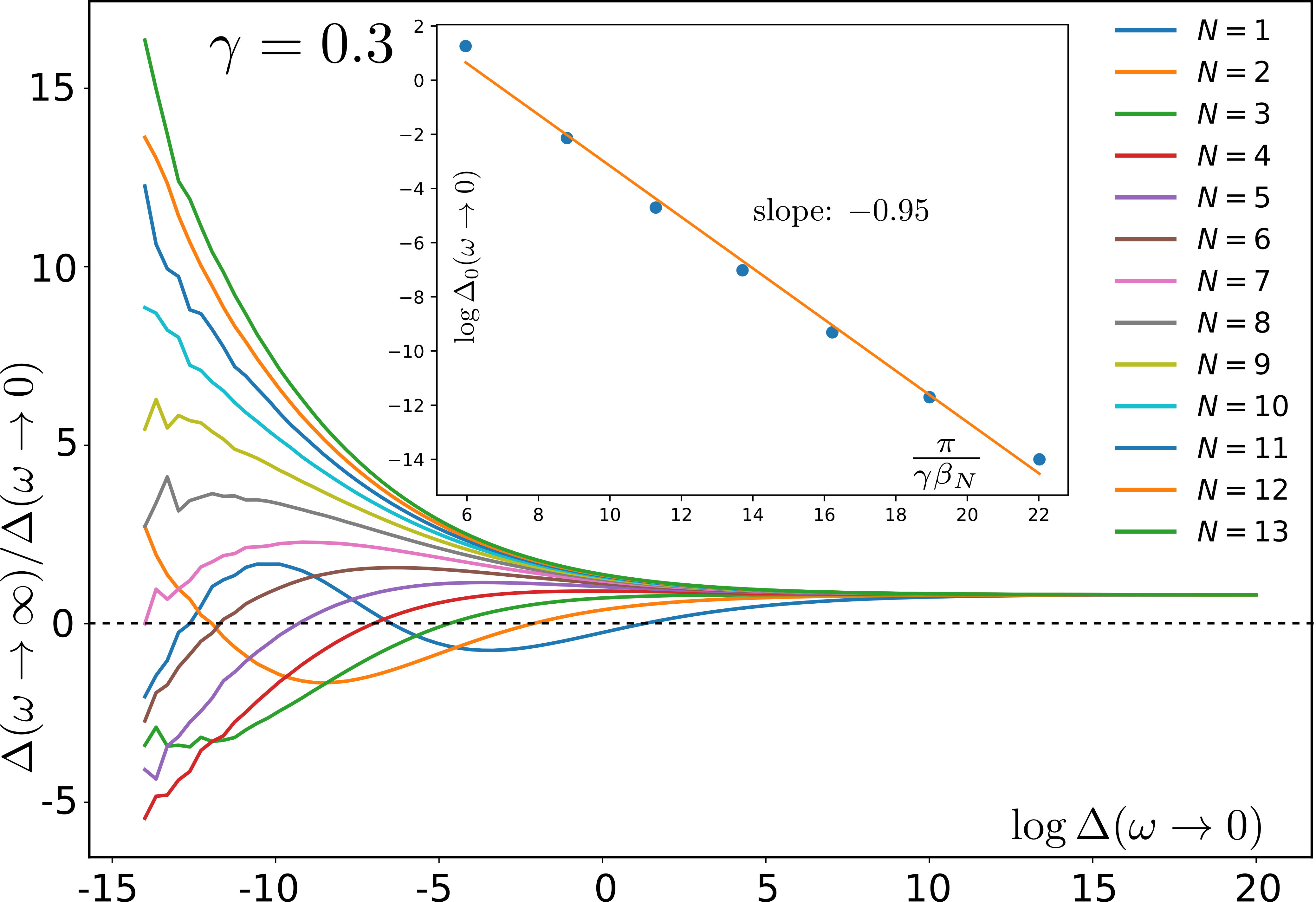

In the left panel of Fig. (15) we collect the results for and different between and , the inset shows a comparison of and , where . We see that the agreement is quite good: the theoretical slope is (see Eq. (84)) and the fitting of numerical data yields the slope .
Finally, in the right panel of Fig. (15) we plot vs for , where is already very small. We see that the gap function flattens at , which is much smaller than the scale at which has a broad maximum. This is again consistent with our qualitative reasoning.
In the subsequent publication (Paper II, Ref.Wu et al. 2020) we collaborate the analysis with the analysis of the linearized gap equation at a finite . We show that for , there exists a discrete set of onset pairing temperatures , and the eigenfunction changes sign times as a function of Matsubara frequency. We argue that these grow in magnitude below , but preserve the number of sign changes, and at coincide with , which we found here.
We note in passing that has a maximum at . The reason for the maximum is that at , a non-zero emerges only at , and , including , scale with . Meanwhile, the onset temperature for the pairing into the state, , is of order . The gap structure reflects this discrepancy: at the lowest frequencies scales with , but the gap at scales with . This gives rise to a maximum at .
VII Conclusions
In this paper we analyzed the competition between two opposing trends in the behavior of interacting fermions near a quantum critical point in a metal: non-Fermi-liquid physics and pairing. Both trends are captured within the model of fermions interacting by exchanging soft bosonic fluctuations of an order parameter, which condenses at the critical point. The non-Fermi liquid behavior is the result of strong, non-analytic self-energy due to boson-mediated scattering near the Fermi surface, the pairing is due to strong attraction in at least one pairing channel, provided by the same soft boson exchange. We considered a class of quantum-critical models with an effective dynamical electron-electron interaction (the -model). In this paper, the first in the series, we considered the case and restricted the analysis to . The limit corresponds to BCS theory without the upper cutoff, but for all finite the interaction drops off at large and the pairing problem is ultra-violet convergent. To parametrically separate the tendencies towards non-Fermi liquid and pairing, we extended the model and introduced the parameter as additional overall factor in the pairing interaction only. At large , the tendency towards non-Fermi liquid normal state at is stronger by , at small the tendency towards pairing is stronger by .
Our analysis brings two conclusions. First, we found that there indeed exists a critical , separating non-Fermi liquid normal state at larger and superconducting state at smaller . The critical for all , such that the original model is superconducting at . Second, we found that the system behavior for is rather unconventional in the sense that there exists an infinite set of solutions of the non-linear gap equation, , , all within the same pairing symmetry. The solutions are topologically distinct: changes sign times as a function of Matsubara frequency . All emerge at , and for their magnitudes scale as , where . The end point of the set, , is the solution of the linearized gap equation at . We obtained the exact analytical solution of the linearized gap equation at and also a highly accurate simple approximate solution for all . In the subsequent paper we analyze the linearized gap equation at a finite and show that there is an infinite set of the onset temperatures for the pairing, , and the corresponding eigenfunctions change sign times as functions of . We argue that these topologically distinct gap functions grow in magnitude below the corresponding , but largely preserve the functional forms and at become that we found in this work.
The sign-preserving solution with has the largest condensation energy and is the global minimum of the condensation energy . All other solutions are local minima. Still, the presence of the infinite set of , including the solution of the linear gap equation for all is a highly non-trivial feature of the pairing at a QCP. In subsequent publications we extend the analysis to and argue that the local minima become more closely spaced with increasing form a continuous set for . We argue that in this case all solutions have equal condensation energy, and superconducting order gets destroyed already at . As the consequence, the true superconducting terminates at , while the onset temperature for the pairing remains finite (see Fig. 2). The two temperatures then must be different for all , including , which we considered here. In between and the system displays pseudogap behavior. We emphasize again that the root to this highly unusual behavior is the existence of the solution of the linearized gap equation for all , rather than only at .
Acknowledgements.
We thank I. Aleiner, B. Altshuler, E. Berg, D. Chowdhury, L. Classen, K. Efetov, R. Fernandes, A. Finkelstein, E. Fradkin, A. Georges, S. Hartnol, S. Karchu, S. Kivelson, I. Klebanov, A. Klein, R. Laughlin, S-S. Lee, G. Lonzarich, D. Maslov, F. Marsiglio, M. Metlitski, W. Metzner, A. Millis, D. Mozyrsky, C. Pepan, V. Pokrovsky, N. Prokofiev, S. Raghu, S. Sachdev, T. Senthil, D. Scalapino, Y. Schattner, J. Schmalian, D. Son, G. Tarnopolsky, A-M Tremblay, A. Tsvelik, G. Torroba, E. Yuzbashyan, J. Zaanen, and particularly R. Combescot, Y. Wang and Y. Wu for useful discussions. The work by AVC was supported by the NSF DMR-1834856.Appendix A The case of small and a finite frequency cutoff
The limit of the model attracted a lot of attention from various sub-communities in physicsRaghu et al. 2015; Wu et al. 2019a; Wang et al. 2017a; Wang et al. 2018; Fitzpatrick et al. 2015b; Metlitski et al. 2015; Mross et al. 2010; Son 1999; *son2 and has been analyzed in both Eliashberg-type and renormalization group approaches. This limit requires extra care because strictly at , the interaction becomes frequency independent, and the pairing problem becomes equivalent to BCS, but without the upper cutoff for the interaction. Meanwhile for any non-zero , the gap equation converges at . More explicit calculation yields (Refs. Metlitski et al. 2015; Wang et al. 2016; Wu et al. 2019a; Yuzbashyan et al. a). This remains finite at any non-zero , but grows with decreasing faster than the exponent.
In this Appendix we consider how the gap equation gets modified if we introduce the upper cutoff for at , i.e., modify to
| (91) |
for , and for . We consider for which . In this case we can expand to first order in and express it for as . The normal state self-energy is . Substituting these and into the equation for the pairing vertex, we obtain
| (92) |
Introducting logarithmic variables , and restricting with the contributions from and , as we did in the derivation of (43), we reduce (92) to
| (93) |
Differentiating twice over and introducing , we obtain
| (94) |
The boundary conditions are ( must vanish at ) and , i.e., . The last condition is set to avoid the divergence in (92) at vanishing . The solution of (94) is
| (95) |
This satisfies the boundary condition provided , i.e., . To satisfy the other boundary condition we choose .
We plot in Fig.16 for and . We see that is an oscillating function of for and an oscillating function of for . For we have, restoring the units of frequency,
| (96) |

The largest frequency for oscillations is . This scale determines the magnitude of the gap . For , . The ratio plays the role of a dimensionless coupling , and can be cast into . This agrees with Refs. Son 1999; *son2; Metlitski et al. 2015. Comparing obtained with and without the cutoff at we see that the analysis of the model without the upper cutoff is valid as long as . At smaller , . We emphasize that even in this case there are an infinite number of solutions
| (97) |
This is valid up to . For larger , relevant in (94) become larger than one, and the formula for changes.
At small and , the ratio is small at , both when is finite and when it is set to infinity. In the first case, the ratio is of order , in the second it is of order . This implies that for the computations , the self-energy can be safely neglected. Once self-energy is neglected, one can easily obtain the differential gap equation for the full in (91), without expanding it to first order in . This allows us to study the crossover between the behavior at finite and infinite .
Introducing, as before, and anticipating that relevant , we find that the equation for for and given by (91), is the same as when , i.e.,
| (98) |
However, now has to satisfy the boundary condition , where . The proper solution of (98) is
| (99) |
In the limit , we use
| (100) |
and obtain
| (101) |
In original variables, and , this reduces, to the leading order in , to
| (102) |
This coincides with (96), up to subleading terms.
In the opposite limit, , we use , , where . Keeping only , we obtain from (99) that the dependence on disappears, and
| (103) |
This coincides with Eq. (52).
The same result can be obtained from the RG equations Metlitski et al. 2015; Wang et al. 2017a. One has to write a set of two RG equations for the two-fermion pairing vertex and the effective 4-fermion pairing interaction . Both depend on the logarithmic scale . To leading order in , the equations for the running and are
| (104) |
The initial condition is
| (105) |
The solution of (104) is and
| (106) |
For (i.e., for small and finite ), relevant values of the arguments of Bessel and Neumann functions are large, and using (100) we find that cancels out, and
| (107) |
The 4-fermion vertex formally diverges at the set of . Using , valid when is finite and , and associating the corresponding with , we reproduce (97).
In the opposite limit, , valid when is kept finite and is set to be sufficiently large, we again use that at small , . Keeping only in (106), we obtain
| (108) |
The 4-fermion vertex now diverges at the set of zeros of , where
| (109) |
where, as before, (we used that for small , . We see that now cancels out, and the condition gives the same set of as for the case when is infinite.
Appendix B Differential gap equation for arbitrary .
The derivation of the differential gap equation, Eq. (43), from the original integral equation is only justified for small . In this appendix we modify the derivation and show that for the modified gap function shows qualitatively the same behavior as the exact even for .
Specifically, we add to the r.h.s of (43) the additional contribution from , where the interaction is strongly peaked at . There is some uncertainty with this contribution as we have to specify the range of integration around . We choose this range to be and keep as a parameter. We assume that for small , , but for , . Adding this contribution to the r.h.s. of Eq. (43) we find that it becomes
| (110) |
where . Introducing instead of , rescaling to and differentiating twice over we obtain differential gap equation in the same form as in (47)
| (111) |
once we identify
| (112) |
Hence, the solution is given by Eq. (53) with instead of .
Eq. (112) determines . At small , , hence, is small and . However, for larger , , and the rescaling is essential. Fig. 12 shows that it brings closer to the exact .
We note in this regard that for and , , and the r.h.s. of (112) becomes of order one if we choose . This is consistent with the fact that tends to a finite value at . Also, the rescaling factor , hence, for , becomes of order . As the consequence, the modified evolves at a non-singular . This is consistent with the behavior of at and (see Fig. 12(e)).
Appendix C The exact solution of the linearized gap equation – the computational details.
In this appendix we present the full details of the computations, leading to the formula for the exact solution of the equation (11). The presentation is self-contained in the sense that it does not use specific notations, introduced in the main text.
C.1 Reformulation of Eq. (11).
We write Eq. (11) as
| (113) |
and use the latter instead of to emphasize that this is a continuous variable.22 2 The method, presented in this appendix, will also work for a generalized version of Eq. (113) with instead of .
We introduce a set of functions
| (114) |
where changes from to and is a convergence factor. It is clear that
We now denote
| (115) |
multiply (113) by , and integrate it over . We obtain
where
| (116) |
From the definition (115) (we also use the fact that is taken to be an even function of frequency) we find
We then have
We now compute the integral
where . At the integral perfectly converges with or without the convergence factor. At we do need the convergence factor, and we assume that is a small positive number. Evaluating the integral we then obtain
| (117) |
and
We now substitute , and use instead of . Then,
| (118) |
Introducing the new function via
| (119) |
we obtain from (118) the equation for in the form
| (120) |
C.2 The functional .
For an infinitesimally small , the free energy difference between the states with and is given by
| (121) |
where we defined to shorten the notations. Taking the first variation of this functional we obtain equation (113) This functional defines our space of functions, namely we must only consider the functions for which is finite.
C.3 Normalizability condition.
C.4 Solution of Eq. (120)
We now show that the normalizable solution of Eq. (120) exists for all . We obtain and use them to obtain the pairing vertex and the gap function . For this purpose we need to first find symmetry properties of in (120).
C.4.1 vs .
The equation (113) is real. So, (i) if an eigenfunction is complex, its complex conjugated must also be an eigenfunction with the same eigenvalue. The eigen value then is double degenerate; (ii) If an eigenvalue is non-degenerate, then the eigenfunction must be real (more precisely, it may have a trivial independent phase.) If the eigenfunction of Eq. (113) is real, then, according to Eqs. (114) and (115), we have
As the function is real and symmetric under the change we have
| (125) |
C.4.2 Periodicity.
C.4.3 Analytical properties.
Let us consider Eq. (120) for arbitrary complex , keeping to be real. This way we define the analytical function . The integral perfectly converges as long as for integer . So the function can only have singularities on the lines . It cannot have poles on these lines, as in this case the integral in the r.h.s. of Eq. (120) would not converge.
Let us return to Eq. (120) and use it to define an analytic function :
(we assume ). The function is related to as
| (127) |
Using the fact that both and are analytic in narrow strip below the real axis, we can express as
| (128) |
This formula must be understood in the sense that to compute , for real , we must first take the limit and then , in which case in the r.h.s. of (128) is below the integration path. The function obviously satisfies the periodicity condition, Eq. (126). It is also clear from (128) that has branch cuts along the lines .
Let us now compute , for real and positive . By Sokhotski-Plemelj theorem: . Hence
which means that
| (129) |
This equation is a particular case of the Riemann-Hilbert problem.
Here, one has to distinguish between the following two cases
- •
(i)] – in this case the expression does not change sign, and
- •
(ii)] – in this case the expression changes sign twice at , where
| (130) |
We consider the two cases separately.
Case (i). : In this case we take the logarithms of the both sides of the equation (129), we then get
So the analytic function has branch cuts along the lines with the jumps given by above formula. According to Sokhotski-Plemelj theorem we have
where the analytic function has no branch cuts or singularities, so it must be a polynomial. In order to find this polynomial, we notice, that the first term in the right hand side does not change if we shift , while must acquire a factor of and must acquire extra . There are only two polynomials that have this property, they are are , so there are two solutions:
| (131) |
Correspondingly, there are two solutions for
| (132) |
where is now real.
Notice, that we have two solutions. One can check, that they are indeed complex conjugated.
As the consequence,
The last integral diverges. The divergence implies that the solutions with are not normalizable and are not the part of the spectrum.
Case (ii). . In this case there are two points (130) where the r.h.s of (129) changes sign. To avoid ambiguity of , we first rewrite (129) as
where is the step function ( and ) Now we take the log of both sides
The is zero for and either or for . Let us introduce two yet unknown functions and , which have values , depending on , and rewrite the equation above as
The Sokhotski-Plemelj theorem now gives
This can be re-expressed as
According to (126), the difference should be equal to independent on . For from (C.4.3) we have
In order for this expression to be independent of , the functions and must be independent of and must be equal to , where is an arbitrary complex constant. We then denote , , where , . The signs of and can be chosen independently. After this, we obtain
| (133) |
Now, we can find the function
| (134) |
(we redefined the constant )
Now, we need to check if the solution (134) is normalizable. For this, we need to verify whether the integral in (124) converges at large . This requires us to compute the real part of the exponent in (134) for . We do this on term by term basis
Combining, we find that the real part of the exponent in (134) is
We see that if we chose , and the minus sign for the term , we get
This guarantees the convergence of the integral in (124).
With this choice of the constants, the function becomes
| (135) |
where, we remind, is defined in (130).
Notice the following: (i) The normalizability of is due to the asymptotic. This absolute value comes from the contribution from the branch cut of the log. This holds only for ; (ii) There exists only one normalizable solution. This means that this must satisfy the condition (125). One can check explicitly that it is indeed so.
C.5 Pairing vertex
We now use from Eq. (135) to compute the function . We recall that is expressed via as
| (136) |
We show that this expression is equivalent to
| (137) |
where
| (138) |
To prove this, we employ the following trick: use
and write
or
Comparing this expression with Eq. (113), we recover (137). Notice, that this proof does not use an explicit form of the function . It does, however, explicitly uses that fact that is the solution of (67).33 3 There is another way to prove (138) which does not use the fact that is a solution of (67), instead it uses the analytical properties of the function .
The gap function is expressed as
| (139) |
C.6 Summary: The steps to obtain the pairing vertex and the gap function for .
The strategy is the following:
- 1.
Evaluate the integral
(140) Notice, that it is real and antisymmetric.
- 2.
Construct the function
(141) - 3.
Compute
(142) - 4.
The exact solutions of the linearized equations for the pairing vertex and the gap function are
(143)
Appendix D Asymptotic expansion at small and large frequencies
To understand the structure of it is instructive to expand it at small and large . One can do this in two ways: expand in the formulas for the exact solution, or perturbatively expand the gap equation (10) order by order in or .
For shortness, we present here the details of the direct perturbative expansion. The point of departure for the expansion in is the solution of (10) without the last term : Re, where
| (144) |
and, we remind, and is the solution of , where is given by (38).
Let us expand the r.h.s. of (10) in and express as Re. The equation for is
| (145) |
There are two types of terms in the r.h.s of (145). The first term is local in the sense that the integral over is ultra-violet and infra-red convergent and is determined by comparable to . Evaluating this term, we obtain
| (146) |
where
| (147) |
and the integration variable .
D.1 Local corrections.
Let us momentarily keep only the local term in the r.h.s. of (145). We label the corresponding portion of as . The functional form of is determined by (146): . Substituting into (145), we find the relation between and :
| (148) |
This analysis can be straightforwardly extended to higher orders in the expansion in . At each other we extract infra-red convergent contribution in the source term by subtracting from a proper number of terms ( , , etc) to make the remaining integral over ultra-violet convergent, and solve for induced by such source terms. The result is
| (149) |
where, we remind, , and
| (150) |
where
| (151) |
Note than are complex numbers. Combining and , we obtain the total local contribution to the pairing vertex Re as
| (152) |
Expressing (152) as the equation for the local contribution to the gap function , we obtain the first term in (75).
At small and , . Evaluating in two orders in , we find a simple expression
| (153) |
Substituting this into (150) and then into (149), using the relation between and , and exponentiating the series to order , we obtain, up to corrections of order ,
| (154) |
where . Eq. (154) and the expansion of coincide with those for , Eqs. (58) and (59). This explicitly confirms that for , .
D.2 Non-local corrections.
We now look at the other terms, which we had to add and subtract at each order to make local contributions ultra-violet convergent. At the leading order in the expansion the additional term in the r.h.s. of Eq. (145) is
| (155) |
This integral is ultra-violet divergent, but the divergence is fictitious because the actual must drop as at large . Accordingly, we cut ultra-violet divergencies at some , which, we argue below, is roughly where changes sign. The separation into local and non-local terms obviously holds only for . The non-local term (155) induces another set of corrections to the bare Re. We label the corresponding non-local part of the full as . By construction, is real. Substituting (155) into (145), adding the complex conjugated term, and adding and subtracting to/from , we obtain the equation for in the form
| (156) |
where
| (157) |
We first notice that Eq. (156) without the term does have the solution , where is the solution of in the interval . For within this range, the integral in the l.h.s. of (156) does not diverge in the infra-red and ultra-violet limits. To satisfy (156) one needs to satisfy also the condition . Substituting our trial solution for and Re into (157), we find that the condition is satisfied for some particular ratio .
This analysis can be extended to higher orders in the perturbation theory. The non-local terms in the r.h.s. of the equation for the pairing vertex appear in the form , where all contain as the overall factor. To cancel all these non-local terms, we choose in the form
| (158) |
where . The terms with are solutions of the same equation (157), but with the proper number of terms subtracted from and added to the term in the r.h.s, to make the integral over in the l.h.s. ultra-violet convergent. We see from Fig. 13 that there is one in each interval that satisfies (157). Substituting this form into the equation for the pairing vertex and collecting non-local terms, we find a set of coupled algebraic equations for with playing the role of source terms. The precise forms of these equations cannot be obtained within perturbative expansion in , and we just have to assume that the solution exists. Reexpressing (158) as the equation for instead of , we reproduce series in (75).
Combining (152) and (158) we see that the r.h.s. of Eq. (75) is the sum of local and non-local contributions
| (159) |
At the largest one can expand in and use as the zero-order solution. The expansion is straightforward and yields Eq. (76).
References
- Monthoux et al. (2007) P. Monthoux, D. Pines, and G. G. Lonzarich, Nature 450, 1177 (2007).
- Scalapino (2012) D. J. Scalapino, Rev. Mod. Phys. 84, 1383 (2012).
- Norman (2014) M. R. Norman, “Novel superfluids,” (Oxford University Press, 2014) Chap. Unconventional superconductivity.
- Maiti and Chubukov (2014) S. Maiti and A. V. Chubukov, “Novel superfluids,” (Oxford University Press, 2014) Chap. Superconductivity from repulsive interaction.
- Keimer et al. (2015) B. Keimer, S. A. Kivelson, M. R. Norman, S. Uchida, and J. Zaanen, Nature 518, 179 (2015).
- Shibauchi et al. (2014) T. Shibauchi, A. Carrington, and Y. Matsuda, Annual Review of Condensed Matter Physics 5, 113 (2014).
- Fernandes and Chubukov (2016) R. M. Fernandes and A. V. Chubukov, Reports on Progress in Physics 80, 014503 (2016).
- Fradkin et al. (2010) E. Fradkin, S. A. Kivelson, M. J. Lawler, J. P. Eisenstein, and A. P. Mackenzie, Annual Review of Condensed Matter Physics 1, 153 (2010).
- Yang et al. (2006) K.-Y. Yang, T. M. Rice, and F.-C. Zhang, Phys. Rev. B 73, 174501 (2006).
- Fratino et al. (2016) L. Fratino, P. Sémon, G. Sordi, and A.-M. S. Tremblay, Scientific Reports 6, 22715 (2016).
- Sachdev (2018) S. Sachdev, Reports on Progress in Physics 82, 014001 (2018).
- Coleman (2015) P. Coleman, Introduction to Many-Body Physics (Cambridge University Press, 2015).
- Mross et al. (2010) D. F. Mross, J. McGreevy, H. Liu, and T. Senthil, Phys. Rev. B 82, 045121 (2010).
- Metlitski et al. (2015) M. A. Metlitski, D. F. Mross, S. Sachdev, and T. Senthil, Phys. Rev. B 91, 115111 (2015).
- Mahajan et al. (2013) R. Mahajan, D. M. Ramirez, S. Kachru, and S. Raghu, Phys. Rev. B 88, 115116 (2013).
- Fitzpatrick et al. (2013) A. L. Fitzpatrick, S. Kachru, J. Kaplan, and S. Raghu, Phys. Rev. B 88, 125116 (2013).
- Fitzpatrick et al. (2014) A. L. Fitzpatrick, S. Kachru, J. Kaplan, and S. Raghu, Phys. Rev. B 89, 165114 (2014).
- Torroba and Wang (2014) G. Torroba and H. Wang, Phys. Rev. B 90, 165144 (2014).
- Fitzpatrick et al. (2015a) A. L. Fitzpatrick, G. Torroba, and H. Wang, Phys. Rev. B 91, 195135 (2015a), and references therein.
- Wang et al. (2018) H. Wang, Y. Wang, and G. Torroba, Phys. Rev. B 97, 054502 (2018).
- Wang et al. (2017a) H. Wang, S. Raghu, and G. Torroba, Phys. Rev. B 95, 165137 (2017a).
- Fitzpatrick et al. (2015b) A. L. Fitzpatrick, S. Kachru, J. Kaplan, S. Raghu, G. Torroba, and H. Wang, Phys. Rev. B 92, 045118 (2015b).
- Millis (1992) A. J. Millis, Phys. Rev. B 45, 13047 (1992).
- Altshuler et al. (1995a) B. L. Altshuler, L. B. Ioffe, A. I. Larkin, and A. J. Millis, Phys. Rev. B 52, 4607 (1995a).
- Sachdev et al. (1995) S. Sachdev, A. V. Chubukov, and A. Sokol, Phys. Rev. B 51, 14874 (1995).
- Abanov et al. (2001a) A. Abanov, A. V. Chubukov, and A. M. Finkel’stein, EPL (Europhysics Letters) 54, 488 (2001a).
- Abanov et al. (2003) A. Abanov, A. V. Chubukov, and J. Schmalian, Advances in Physics 52, 119 (2003).
- Abanov and Chubukov (1999) A. Abanov and A. V. Chubukov, Phys. Rev. Lett. 83, 1652 (1999).
- Abanov et al. (2001b) A. Abanov, A. V. Chubukov, and J. Schmalian, Journal of Electron spectroscopy and related phenomena 117, 129 (2001b).
- Abanov et al. (2008) A. Abanov, A. V. Chubukov, and M. R. Norman, Phys. Rev. B 78, 220507 (2008).
- Sachdev et al. (2009) S. Sachdev, M. A. Metlitski, Y. Qi, and C. Xu, Phys. Rev. B 80, 155129 (2009).
- Moon and Sachdev (2009) E. G. Moon and S. Sachdev, Phys. Rev. B 80, 035117 (2009).
- Sachdev et al. (2019) S. Sachdev, H. D. Scammell, M. S. Scheurer, and G. Tarnopolsky, Phys. Rev. B 99, 054516 (2019).
- Vojta and Sachdev (1999) M. Vojta and S. Sachdev, Phys. Rev. Lett. 83, 3916 (1999).
- Wang and Chubukov (2013a) Y. Wang and A. V. Chubukov, Phys. Rev. Lett. 110, 127001 (2013a).
- Efetov et al. (2013) K. B. Efetov, H. Meier, and C. Pepin, Nature Physics 9, 442 (2013).
- Meier et al. (2014) H. Meier, C. Pépin, M. Einenkel, and K. B. Efetov, Phys. Rev. B 89, 195115 (2014).
- Efetov (2015) K. B. Efetov, Phys. Rev. B 91, 045110 (2015).
- Tsvelik (2017) A. M. Tsvelik, Phys. Rev. B 95, 201112 (2017).
- Metlitski and Sachdev (2010a) M. A. Metlitski and S. Sachdev, Phys. Rev. B 82, 075128 (2010a).
- Dalidovich and Lee (2013) D. Dalidovich and S.-S. Lee, Phys. Rev. B 88, 245106 (2013).
- Lee (2018) S.-S. Lee, Annual Review of Condensed Matter Physics 9, 227 (2018).
- Bauer and Sachdev (2015) J. Bauer and S. Sachdev, Phys. Rev. B 92, 085134 (2015).
- Castellani et al. (1995) C. Castellani, C. Di Castro, and M. Grilli, Phys. Rev. Lett. 75, 4650 (1995).
- Perali et al. (1996) A. Perali, C. Castellani, C. Di Castro, and M. Grilli, Phys. Rev. B 54, 16216 (1996).
- Andergassen et al. (2001) S. Andergassen, S. Caprara, C. Di Castro, and M. Grilli, Phys. Rev. Lett. 87, 056401 (2001).
- Wang and Chubukov (2015) Y. Wang and A. V. Chubukov, Phys. Rev. B 92, 125108 (2015).
- Chowdhury and Sachdev (2014a) D. Chowdhury and S. Sachdev, Phys. Rev. B 90, 245136 (2014a).
- Khodas et al. (2010) M. Khodas, H. B. Yang, J. Rameau, P. D. Johnson, A. M. Tsvelik, and T. M. Rice, ArXiv:1007.4837 (2010).
- Konik et al. (2010) R. M. Konik, T. M. Rice, and A. M. Tsvelik, Phys. Rev. B 82, 054501 (2010).
- Khodas and Tsvelik (2010) M. Khodas and A. M. Tsvelik, Phys. Rev. B 81, 094514 (2010).
- Chubukov and Tsvelik (2007) A. V. Chubukov and A. M. Tsvelik, Phys. Rev. B 76, 100509 (2007).
- Metzner et al. (2003) W. Metzner, D. Rohe, and S. Andergassen, Phys. Rev. Lett. 91, 066402 (2003).
- Dell’Anna and Metzner (2006) L. Dell’Anna and W. Metzner, Phys. Rev. B 73, 045127 (2006).
- Vilardi et al. (2018) D. Vilardi, C. Taranto, and W. Metzner, arXiv:1810.02290 and references therein (2018).
- Holder and Metzner (2015) T. Holder and W. Metzner, Phys. Rev. B 92, 245128 (2015).
- Yamase et al. (2016) H. Yamase, A. Eberlein, and W. Metzner, Phys. Rev. Lett. 116, 096402 (2016).
- Sordi et al. (2012) G. Sordi, P. Simon, K. Haule, and A.-M. S. Tremblay, Phys. Rev. Lett. 108, 216401 (2012).
- Chubukov and Wölfle (2014) A. V. Chubukov and P. Wölfle, Phys. Rev. B 89, 045108 (2014).
- Altshuler et al. (1995b) B. L. Altshuler, L. B. Ioffe, and A. J. Millis, Phys. Rev. B 52, 5563 (1995b).
- Bergeron et al. (2012) D. Bergeron, D. Chowdhury, M. Punk, S. Sachdev, and A.-M. S. Tremblay, Phys. Rev. B 86, 155123 (2012).
- Wang and Chubukov (2013b) Y. Wang and A. Chubukov, Phys. Rev. B 88, 024516 (2013b).
- Kim et al. (2008) E.-A. Kim, M. J. Lawler, P. Oreto, S. Sachdev, E. Fradkin, and S. A. Kivelson, Phys. Rev. B 77, 184514 (2008).
- Lawler and Fradkin (2007) M. J. Lawler and E. Fradkin, Phys. Rev. B 75, 033304 (2007).
- Berg et al. (2009) E. Berg, E. Fradkin, and S. A. Kivelson, Phys. Rev. B 79, 064515 (2009).
- Soto-Garrido and Fradkin (2014) R. Soto-Garrido and E. Fradkin, Phys. Rev. B 89, 165126 (2014).
- Bonesteel et al. (1996) N. E. Bonesteel, I. A. McDonald, and C. Nayak, Phys. Rev. Lett. 77, 3009 (1996).
- Oganesyan et al. (2001) V. Oganesyan, S. A. Kivelson, and E. Fradkin, Phys. Rev. B 64, 195109 (2001).
- Sur and Lee (2015) S. Sur and S.-S. Lee, Phys. Rev. B 91, 125136 (2015).
- Punk (2015) M. Punk, Phys. Rev. B 91, 115131 (2015), and references therein.
- Rech et al. (2006) J. Rech, C. Pépin, and A. V. Chubukov, Phys. Rev. B 74, 195126 (2006).
- Lee (2009) S.-S. Lee, Phys. Rev. B 80, 165102 (2009).
- Metlitski and Sachdev (2010b) M. A. Metlitski and S. Sachdev, Phys. Rev. B 82, 075127 (2010b).
- Lederer et al. (2015) S. Lederer, Y. Schattner, E. Berg, and S. A. Kivelson, Phys. Rev. Lett. 114, 097001 (2015).
- Maslov and Chubukov (2012) D. L. Maslov and A. V. Chubukov, Phys. Rev. B 86, 155137 (2012).
- Chubukov and Maslov (2012) A. V. Chubukov and D. L. Maslov, Phys. Rev. B 86, 155136 (2012).
- Maslov and Chubukov (2010) D. L. Maslov and A. V. Chubukov, Phys. Rev. B 81, 045110 (2010).
- Maslov and Chubukov (2009) D. L. Maslov and A. V. Chubukov, Phys. Rev. B 79, 075112 (2009).
- You et al. (2016) Y. You, G. Y. Cho, and E. Fradkin, Phys. Rev. B 93, 205401 (2016).
- Wang et al. (2001) Z. Wang, W. Mao, and K. Bedell, Phys. Rev. Lett. 87, 257001 (2001).
- Roussev and Millis (2001) R. Roussev and A. J. Millis, Phys. Rev. B 63, 140504 (2001).
- Chubukov et al. (2003) A. V. Chubukov, A. M. Finkel’stein, R. Haslinger, and D. K. Morr, Phys. Rev. Lett. 90, 077002 (2003).
- Lederer et al. (2017) S. Lederer, Y. Schattner, E. Berg, and S. A. Kivelson, Proceedings of the National Academy of Sciences 114, 4905 (2017).
- Klein et al. (2019) A. Klein, Y.-M. Wu, and A. V. Chubukov, npj Quantum Materials 4, 55 (2019).
- Klein and Chubukov (2018) A. Klein and A. Chubukov, Phys. Rev. B 98, 220501 (2018).
- Bok et al. (2016) J. M. Bok, J. J. Bae, H.-Y. Choi, C. M. Varma, W. Zhang, J. He, Y. Zhang, L. Yu, and X. J. Zhou, Science Advances 2 (2016), 10.1126/sciadv.1501329.
- Lee (1989) P. A. Lee, Phys. Rev. Lett. 63, 680 (1989).
- Blok and Monien (1993) B. Blok and H. Monien, Phys. Rev. B 47, 3454 (1993).
- Nayak and Wilczek (1994) C. Nayak and F. Wilczek, Nuclear Physics B 417, 359 (1994).
- Altshuler et al. (1994) B. L. Altshuler, L. B. Ioffe, and A. J. Millis, Phys. Rev. B 50, 14048 (1994).
- Kim et al. (1994) Y. B. Kim, A. Furusaki, X.-G. Wen, and P. A. Lee, Phys. Rev. B 50, 17917 (1994).
- Raghu et al. (2015) S. Raghu, G. Torroba, and H. Wang, Phys. Rev. B 92, 205104 (2015).
- Moon and Chubukov (2010) E.-G. Moon and A. Chubukov, Journal of Low Temperature Physics 161, 263 (2010).
- Khveshchenko and Shively (2006) D. V. Khveshchenko and W. F. Shively, Phys. Rev. B 73, 115104 (2006).
- She and Zaanen (2009) J.-H. She and J. Zaanen, Phys. Rev. B 80, 184518 (2009).
- She et al. (2010) J.-H. She, J. Zaanen, A. R. Bishop, and A. V. Balatsky, Phys. Rev. B 82, 165128 (2010).
- Wang et al. (2016) Y. Wang, A. Abanov, B. L. Altshuler, E. A. Yuzbashyan, and A. V. Chubukov, Phys. Rev. Lett. 117, 157001 (2016).
- Lee et al. (2018) T.-H. Lee, A. Chubukov, H. Miao, and G. Kotliar, Phys. Rev. Lett. 121, 187003 (2018).
- Wu et al. (2019a) Y.-M. Wu, A. Abanov, and A. V. Chubukov, Phys. Rev. B 99, 014502 (2019a).
- Wu et al. (2019b) Y.-M. Wu, A. Abanov, Y. Wang, and A. V. Chubukov, Phys. Rev. B 99, 144512 (2019b).
- Abanov et al. (2019) A. Abanov, Y.-M. Wu, Y. Wang, and A. V. Chubukov, Phys. Rev. B 99, 180506 (2019).
- Yuzbashyan et al. (a) E. A. Yuzbashyan, A. V. Chubukov, A. Abanov, and B. L. Altshuler, “Non BCS pairing near a quantum phase transition – effective mapping to a spin chain,” (a), in preparation.
- Patel and Sachdev (2019) A. A. Patel and S. Sachdev, Phys. Rev. Lett. 123, 066601 (2019).
- Esterlis and Schmalian (2019) I. Esterlis and J. Schmalian, Physical Review B 100 (2019), 10.1103/physrevb.100.115132.
- Wang (2020) Y. Wang, Phys. Rev. Lett. 124, 017002 (2020).
- Hauck et al. (2019) D. Hauck, M. J. Klug, I. Esterlis, and J. Schmalian, arXiv 1911.04328 (2019).
- Chowdhury and Berg (2020) D. Chowdhury and E. Berg, Phys. Rev. Research 2, 013301 (2020).
- Combescot (1995) R. Combescot, Phys. Rev. B 51, 11625 (1995).
- Bergmann and Rainer (1973) G. Bergmann and D. Rainer, Z. Physik 263, 59 (1973).
- Allen and Rainer (1991) P. B. Allen and D. Rainer, Nature 349, 396 EP (1991).
- Allen and Dynes (1975) P. B. Allen and R. C. Dynes, Phys. Rev. B 12, 905 (1975).
- Marsiglio et al. (1988) F. Marsiglio, M. Schossmann, and J. P. Carbotte, Phys. Rev. B 37, 4965 (1988).
- Marsiglio and Carbotte (1991) F. Marsiglio and J. P. Carbotte, Phys. Rev. B 43, 5355 (1991), for more recent results see F. Marsiglio and J.P. Carbotte, “Electron-Phonon Superconductivity”, in “The Physics of Conventional and Unconventional Superconductors”, Bennemann and Ketterson eds., Springer-Verlag, (2006) and references therein.
- Karakozov et al. (1991) A. Karakozov, E. Maksimov, and A. Mikhailovsky, Solid State Communications 79, 329 (1991).
- Chubukov et al. (2020a) A. V. Chubukov, A. Abanov, I. Esterlis, and S. A. Kivelson, Annals of Physics 417, 168190 (2020a), eliashberg theory at 60: Strong-coupling superconductivity and beyond.
- Son (1999) D. T. Son, Phys. Rev. D 59, 094019 (1999).
- Chubukov and Schmalian (2005) A. V. Chubukov and J. Schmalian, Phys. Rev. B 72, 174520 (2005).
- Yang et al. (2011) S.-X. Yang, H. Fotso, S.-Q. Su, D. Galanakis, E. Khatami, J.-H. She, J. Moreno, J. Zaanen, and M. Jarrell, Phys. Rev. Lett. 106, 047004 (2011).
- Gerlach et al. (2017) M. H. Gerlach, Y. Schattner, E. Berg, and S. Trebst, Phys. Rev. B 95, 035124 (2017).
- Schattner et al. (2016) Y. Schattner, S. Lederer, S. A. Kivelson, and E. Berg, Phys. Rev. X 6, 031028 (2016).
- Wang et al. (2017b) X. Wang, Y. Schattner, E. Berg, and R. M. Fernandes, Phys. Rev. B 95, 174520 (2017b).
- Berg et al. (2019) E. Berg, S. Lederer, Y. Schattner, and S. Trebst, Annual Review of Condensed Matter Physics 10, 63 (2019).
- Haule and Kotliar (2007) K. Haule and G. Kotliar, Phys. Rev. B 76, 104509 (2007).
- Xu et al. (2017) W. Xu, G. Kotliar, and A. M. Tsvelik, Phys. Rev. B 95, 121113 (2017).
- Georges et al. (2013) A. Georges, L. d. Medici, and J. Mravlje, Annu. Rev. Condens. Matter Phys. 4, 137 (2013).
- Wu et al. (2017) W. Wu, M. Ferrero, A. Georges, and E. Kozik, Phys. Rev. B 96, 041105 (2017).
- Eliashberg (1960) G. M. Eliashberg, JETP 11, 696 (1960), [ZhETF, 38, 966, (1960)].
- Chubukov et al. (2020b) A. V. Chubukov, A. Abanov, Y. Wang, and Y.-M. Wu, Annals of Physics 417, 168142 (2020b), eliashberg theory at 60: Strong-coupling superconductivity and beyond.
- Yuzbashyan et al. (b) E. A. Yuzbashyan, A. V. Chubukov, A. Abanov, and B. L. Altshuler, “Non BCS pairing near a quantum phase transition – the case of large ,” (b), in preparation.
- Simard et al. (2019) O. Simard, C.-D. Hébert, A. Foley, D. Sénéchal, and A.-M. S. Tremblay, Phys. Rev. B 100, 094506 (2019).
- Linder and Balatsky (2019) J. Linder and A. V. Balatsky, Rev. Mod. Phys. 91, 045005 (2019).
- Yang and Sondhi (2000) K. Yang and S. L. Sondhi, Phys. Rev. B 62, 11778 (2000).
- Wu et al. (2020) Y.-M. Wu, A. Abanov, Y. Wang, and A. V. Chubukov, Phys. Rev. B (2020), in review.
- Haslinger and Chubukov (2003) R. Haslinger and A. V. Chubukov, Phys. Rev. B 68, 214508 (2003).
- (135) In obtaining the Eliashberg equations we assumed that states away from the Fermi surface are irrelevant for the pairing and NFL behavior, and extended the integration over momenta to infinite limits. In this situation, fermionic self-energy is real. If the momentum integration over holds in finite and non-symmetric limits, has both real and imaginary components. The same holds in SYK-type models at a non-zero chemical potential (see Ref. Gu_2020 and references therein).
- Khveshchenko (2009) D. V. Khveshchenko, Journal of Physics: Condensed Matter 21, 075303 (2009).
- Chowdhury and Sachdev (2014b) D. Chowdhury and S. Sachdev, Phys. Rev. B 90, 134516 (2014b).
- Klein et al. (2020) A. Klein, Y. Schattner, E. Berg, and A. V. Chubukov, arXiv:2003.09431 (2020).
- Xu et al. (2020) X. Y. Xu, A. Klein, K. Sun, A. V. Chubukov, and Z. Y. Meng, arXiv:2003.11573 (2020).
- Millis and Monien (1996) A. J. Millis and H. Monien, Phys. Rev. B 54, 16172 (1996).
- Eschrig (2006) M. Eschrig, Advances in Physics 55, 47 (2006), https://doi.org/10.1080/00018730600645636 .
- Abanov et al. (2002) A. Abanov, A. V. Chubukov, M. Eschrig, M. R. Norman, and J. Schmalian, Physical Review Letters 89, 177002 (2002).
- Abanov and Chubukov (2000) A. Abanov and A. Chubukov, Physica B 280, 189 (2000).
- Luttinger and Ward (1960) J. M. Luttinger and J. C. Ward, Phys. Rev. 118, 1417 (1960).
- Wada (1964) Y. Wada, Phys. Rev. 135, A1481 (1964).
- Bardeen and Stephen (1964) J. Bardeen and M. Stephen, Phys. Rev. 136, A1485 (1964).
- Abrikosov et al. (1965) A. A. Abrikosov, L. P. Gorkov, and I. E. Dzyaloshinski, Methods of Quantum Feld Theory in Statistical Physics (Pergamon Oxford, 1965).
- Liu et al. (2011) H. Liu, J. McGreevy, and D. Vegh, Phys. Rev. D 83, 065029 (2011).
- Cortez et al. (2011) J. Cortez, G. A. Mena Marugán, J. Olmedo, and J. M. Velhinho, Phys. Rev. D 83, 025002 (2011).
- Kim et al. (2019) J. Kim, I. R. Klebanov, G. Tarnopolsky, and W. Zhao, Phys. Rev. X 9, 021043 (2019).
- (151) The method, presented in this appendix, will also work for a generalized version of Eq. (113) with instead of .
- (152) There is another way to prove (138) which does not use the fact that is a solution of (67), instead it uses the analytical properties of the function .