Dissociation of heavy quarkonia in a weak magnetic field
Mujeeb Hasan†11 1 mhasan@ph.iitr.ac.in and Binoy Krishna Patra† 22 2 binoy@ph.iitr.ac.in
† Department of Physics, Indian Institute of Technology Roorkee, Roorkee 247 667, India
PACS: 12.39.-x,11.10.St,12.38.Mh,12.39.Pn
12.75.N, 12.38.G
Keywords: Thermal QCD; Weak magnetic field;
Resummed propagator; Dielectric permittivity; Heavy quark potential;
Abstract
We examined the effects of the weak magnetic field on the properties of heavy quarkonia immersed in a thermal medium of quarks and gluons and studied how the magnetic field affects the quasi-free dissociation of quarkonia in the aforementioned medium. For that purpose, we have revisited the general structure of gluon self-energy tensor in the presence of a weak magnetic field in thermal medium and obtained the relevant structure functions using the imaginary-time formalism. The structure functions give rise to the real and imaginary parts of the resummed gluon propagator, which further give the real and imaginary parts of the dielectric permittivity. The real and imaginary parts of the dielectric permittivity will be used to evaluate the real and imaginary parts of the complex heavy quark potential. We have observed that the real-part of the potential is found to be more screened, whereas the magnitude of the imaginary-part of the potential gets increased on increasing the value of both temperature and magnetic field. In addition to this, we have observed that the real-part gets slightly more screened while the imaginary part gets increased in the presence of a weak magnetic field as compared to their counterparts in the absence of a magnetic field (pure thermal). The increase in the screening of the real-part of the potential leads to the decrease of binding energies of and , whereas the increase in the magnitude of the imaginary part leads to the increase of thermal width with the temperature and magnetic field both. Also the binding energy and thermal width in the presence of weak magnetic field become smaller and larger, respectively, as compared to that in the pure thermal case. With the observations of binding energy and thermal width in hands, we have finally obtained the dissociation temperatures for and , which become slightly lower in the presence of weak magnetic field. For example, with the and are dissociated at and , respectively, whereas with they dissociated at slightly lower value and , respectively. This observation leads to the slightly early dissociation of quarkonia because of the presence of a weak magnetic field.
1 Introduction
Lattice QCD predicted that at sufficiently high temperatures and/or densities the quarks and gluons confined inside hadrons get deconfined into a medium of quarks and gluons coined as quark-gluon Plasma. In the last few decades a large number of experiment has been involved in identifying this new state of matter in ultrarelativistic heavy-ion collisions (URHICs) at RHIC and LHC. However, for the noncentral events in URHICs, a strong magnetic field is generated at the very early stages of the collisions due to very high relative velocities of the spectator quarks with respect to the fireball. Depending on the centralities of the collisions, the strength of the magnetic fields may vary from ( Gauss) at RHIC to 10 at LHC [1, 2]. Motivated by this, in the recent past many theoretical works have started emerging to explore the effects of this strong magnetic field on the various QCD phenomena [3, 4, 5, 6]. Earlier the nascent strong magnetic field was thought to decay very fast with time, resulting the magnetic field of weaker strength. However, it was later found that the realistic estimates of electrical conductivity of the medium may elongate the life-time of the magnetic field [7, 8, 9]. It thus becomes imperative to investigate the effects of both strong and weak magnetic field on the signature of the novel matter produced in URHICs.
The heavy quarkonia is one of the probe to study the properties of nuclear matter under extreme condition of temperature and magnetic field, because the heavy quark pairs are formed in URHICs on a very short time-scale (where is the mass of the charm or bottom quark), which is similar to the time-scale at which the magnetic field is generated. Therefore the study of the effects of magnetic field on the properties of heavy quarkonia is worth of investigation. We have recently studied the properties of quarkonia in strong magnetic field. However, as we know the quarkonia, the physical resonances of states, are formed in the plasma frame at a time, (=), which is order of depending on the resonances and their momenta. By the time elapsed, the magnetic field may become weak, so in our present study, we aim to understand theoretically the properties of heavy quarkonia and their dissociation in the presence of weak magnetic field (, , where () is the absolute electric charge (mass) of the -th quark flavour). As we know that, in order to study the dissociation of quarkonia the perturbative computation of heavy quarkonium potential is needed.
Our understanding of heavy quarkonium has taken a major step forward in computing effective field theories (EFT) from the underlying theory - QCD, such as non-relativistic QCD (NRQCD)[10] and potential NRQCD [11], which are synthesized successively by separating the intrinsic scales of heavy quark bound states (e.g. mass, velocity, binding energy) as well as the thermal medium-related scales (e.g. , , ) in the weak-coupling system, in overall comparison with . However, in the relativistic collisions that are created at URHICs, the separation of scales in an EFT is not always apparent, meaning it is often difficult to construct a potential model. An alternative approach is a first-principle lattice QCD simulation in which one studies spectral functions derived from Euclidean meson correlation [12]. The construction of spectral functions, however, is problematic because the temporal range at large temperatures decreases. For this reason studies of quarkonia using finite temperature potential models are useful as a complement to lattice studies. The perturbative computations of the potential at high temperatures show that the potential of is complex [13], where the real part is screened due to the existence of deconfined color charges [14] and the imaginary part [15] assigns the thermal width to the resonance. Therefore the physics of quarkonium dissociation in a medium has been refined in the last two decades, where the resonances were initially thought to be dissociated when the screening is strong enough, i.e. the real-part of the potential is too weak to keep the pair together. Nowadays, the dissociation is thought to be primarily because of the widening of the resonance width arising either from the inelastic parton scattering mechanism mediated by the spacelike gluons, known as Landau damping [13] or from the gluo-dissociation process during which color singlet state undergoes into a color octet state by a hard thermal gluon [16]. The latter processes take precedence when the medium temperature is lower than the binding energy of the particular resonance. This dissociates the quarkonium even at lower temperatures where the probability of color screening is negligible. Recently one of us estimated the imaginary-part of the potential perturbatively, where the inclusion of a confining string term makes the (magnitude) imaginary component smaller [17, 18], compared to the medium modification of the perturbative term alone [19]. Gauge-gravity duality also indicates that in strong coupling limit the potential also develops an imaginary component beyond a critical separation of pair [20, 21]. Moreover lattice studies have also shown that the potential may have a sizable imaginary part [22]. There are, however, other processes which may cause the depopulation of the resonance states either through the transition from ground state to the excited states during the non adiabatic evolution of quarkonia [23] or through the swelling or shrinking of states due to the Brownian motion of states in the parton plasma [24]. Very recently the change in the properties of heavy quarkonia immersed in a weakly-coupled thermal QCD medium has been described by HTL permittivity [25]. They used the generalized Gauss law in conjunction to linear response theory to obtain the real and imaginary parts of the heavy quark potential, where a logarithmic divergence in imaginary part is found due to string contribution at large . They have circumvented by regularizing weak infrared diverging () term in the resummed gluon propagator by choosing the regulation scale in terms of Debye mass. There is another recent work [26], where a nonperturbative term induced by the dimension two gluon condensate besides the usual HTL resummed contribution is included in the resummed gluon propagator to obtain the string contribution in the potential, in addition to the Karsch Mehr Satz (KMS) potential [27].
The abovementioned studies are attributed for a thermal medium in the absence of a magnetic field. However, as mentioned earlier that a magnetic field is also generated in the heavy ion collisions, thus the influence of a homogeneous and constant external magnetic field on the heavy meson spectroscopy has been investigated quantum mechanically subjected to a three-dimensional harmonic potential and Cornell potential plus spin-spin interaction term [28, 29]. Further, the effect of a constant uniform magnetic field on the static quarkonium potential at zero and finite temperature [30] and on the screening masses [31] have been investigated. The momentum diffusion coefficients of heavy quarks in a strong magnetic field along the directions parallel and perpendicular to the magnetic field at the leading order in QCD coupling constant has been studied [32]. Recently we have explored the effects of strong magnetic field on the properties of the heavy-quarkonium in finite temperature by computing the real part of the potential [33] in the framework of perturbative thermal QCD and studied the dissociation of heavy quarkonia due to the color screening. Successively, we made an attempt to study the dissociation of heavy quarkonia due to Landau damping in presence of strong magnetic field by calculating the real and imaginary parts of the heavy quark potential in presence of strong magnetic field [34]. The complex heavy quark potential in presence of strong magnetic field has also been obtained in [35]. Very recently we have also investigated the strong magnetic field-induced anisotropic interaction in heavy quark bound states [36]. The effects of strong magnetic field on the wakes in the induced charge density and in the potential due to the passage of highly energetic partons through a thermal QCD medium has also been investigated [37]. Recently, the dispersion spectra of a gluon in hot QCD medium in presence of strong as well as weak magnetic field limit is studied [38]. The effect of the strong magnetic field on the collisional energy loss of heavy quark moving in a magnetized thermal partonic medium has been studied [39]. Also the anisotropic momentum diffusion and the drag coefficients of heavy quarks have been computed in a strongly magnetized quark-gluon plasma beyond the static limit within the framework of Langevindynamics [40].
In the present study, we aim to obtain the complex heavy quark anti-quark potential in an environment of temperature and weak magnetic field. For that purpose, we first start with the evaluation of gluon self energy in the similar environment using the imaginary-time formalism. As the quark-loop is only affected with the magnetic field thus, the quark-loop in the said environment is now dictated by both the scales namely the magnetic field as well as the temperature, whereas for the gluon-loop, the temperature is the only available scale in the medium as the gluon-loop is not affected with the magnetic field. Furthermore, we have revisited the general structure of gluon self energy tensor in presence of weak magnetic field in thermal medium and obtained the relevant structure functions. Hence the real and imaginary parts of the resummed gluon propagator have been obtained, which give the real and imaginary parts of the dielectric permittivity. The real and imaginary parts of the dielectric permittivity will inturn give the real and imaginary parts of the complex heavy quark potential. The real part of the potential is used in the Schrödinger equation to obtain the binding energy of heavy quarkonia whereas the imaginary part is used to calculate the thermal width. Finally, we have obtained the dissociation temperatures of heavy quarkonia and studied how the dissociation temperatures get affected in presence of magnetic field.
Thus, our work proceeds as follows. In section 2, we will calculate the gluon self energy in a weak magnetic field wherein, we will discuss the general structure of gluon self energy and resummed gluon propagator at finite temperature in presence of weak magnetic field and will calculate the relevant form factors in subsection 2.1 and subsection 2.2, respectively. Thus, the real and imaginary parts of the resummed gluon propagator will give the real and imaginary parts of the dielectric permittivity in subsection 3.1, which gives the real and imaginary parts of complex heavy quark potential in subsection 3.2. We will use the real and imaginary parts of the potential to obtain the binding energy and thermal width in subsection 4.1 and 4.2, respectively, which will then give the dissociation temperatures of heavy quarkonia in subsection 4.3. Finally, we will conclude our findings in section 5.
2 Gluon self energy in a weak magnetic field
In this section we will evaluate the gluon self energy in a weak magnetic field. As we know that for the evaluation of gluon self energy, we need to evaluate both the quark loop and gluon loop contributions in presence of weak magnetic field. Because of weak magnetic field, only the quark loop will get affected whereas the gluon loop remain as such. Now, we will first start with the quark-loop contribution to gluon self energy
| (1) | |||||
where and . The is the quark propagator in a weak magnetic field which can be written upto order of as [41]
| (2) |
where and are the mass and charge of the flavor quark. According to the following choice of metric tensors,
the four-momentum suitable in a magnetic field directed along the axis, , is given by
| (3) | |||||
| (4) | |||||
| (5) | |||||
| (6) |
The above Eq.(2) can be recast in the following form
| (7) |
where is the contribution of the order , is the contribution of the order and is the contribution of the order . Using Eq.(7), the Eq.(1) can be written as
| (8) |
After simplifying, the above gluon self energy given by Eq.(8) can be expressed as follows
| (9) |
where
| (10) | |||||
| (11) | |||||
| (12) |
The term is of the order , where and both are of the order . The term which is of the order vanishes. Substituting the values of , and in Eq.(10), Eq.(11) and Eq.(12) by comparing Eq.(2) with Eq.(7), we get
| (13) | |||||
| (14) | |||||
| (15) | |||||
where
| (16) |
Here the strong coupling runs with the magnetic field and temperature both, which is recently obtained in [42]
| (17) |
with
| (18) |
where is set at , and .
Before evaluating further, we will first discuss the structure of gluon self energy in thermal medium in presence of weak magnetic field in the next subsection.
2.1 Structure of gluon self energy and resummed gluon propagator for thermal medium in the presence of weak magnetic field
In this subsection, we will briefly discuss the general structure of gluon self energy tensor and resummed gluon propagator for thermal medium in the presence of weak magnetic field. The general structure of gluon self energy in a thermal medium defined by the heat bath in local rest frame, and in the presence of magnetic field directed along the -direction, is recently obtained as follows [38]
| (19) |
where
| (20) | |||||
| (21) | |||||
| (22) | |||||
| (23) |
the four vectors and used in the construction of above tensors are defined as follows
| (24) | |||||
| (25) |
where and . Using the properties of projection tensors, the form factors appear in (19) can be obtained as
| (26) | |||||
| (27) | |||||
| (28) | |||||
| (29) |
Now we can obtained the resummed gluon propagator in thermal medium in presence of weak magnetic field. The general form of the resummed gluon propagator in Landau gauge can be written as [38]
| (30) |
The point to be noted here is that, we required only the “00”-component of resummed gluon propagator for deriving the heavy quark potential. Hence the “00”-component of the propagator can be obtained as
| (31) |
where . Now we will obtained the form factors appear in the above propagator (31). We will first start with the form factor , which can be obtained using Eq.(29) with Eq.(9) as
| (32) |
where is of the order of and is of the order of . An important point to be noted here is that the zero magnetic field contribution of form factor vanishes, that is , whereas gives the contribution of order . However the contribution of form factor in the denominator of the propagator (31) appear as , which becomes of the order of . Since in the current theoretical calculation we are considering contribution upto , so we can neglect the contribution appear from the form factor . Thus, the “00”-component of resummed gluon propagator upto can be written as
| (33) |
so we end up with only one form factor , which we will evaluate in the next subsection.
2.2 Real and imaginary parts of the form factor
In this subsection, we will calculate the real and imaginary parts of the form factor . Using Eq.(26), the form factor can be evaluated as follows
| (34) | |||||
where we have used transversality condition , to arrive at Eq. (34). Thus using Eq.(9), the form factor b can be written upto as
| (35) |
where the form factors and are defined as follows
| (36) | |||||
| (37) |
Form factor (order of ):
Here we will solve the form factor . Using
Eq.(36), the form factor can be
written as
| (38) | |||||
Now we will solve the form factor using the imaginary-time formalism, the detailed calculation for which has been shown in appendix A. Thus, the real and imaginary parts of the form factor in the static limit are given as follows
| (39) | |||||
| (40) |
Now we will evaluate the gluonic contribution. The temporal component of gluon self energy due to the gluon-loop contribution can be calculated as [43, 44],
| (41) |
which gives the real and imaginary parts of form factor due to the gluonic contribution in the static limit
| (42) | |||||
| (43) |
Now we add the quark and gluon-loop contributions together to obtain the real and imaginary parts of form factor in the static limit as follows
| (44) | |||||
| (45) |
Thus we can see that the form factor is independent of the magnetic field as it is and depends only on the temperature of the medium. This form factor coincides with the HTL form factor in absence of the magnetic field [43, 44].
Form factor (order of ):
Here we will discuss the form factor , which is of the
order of . Using Eq.(37), the
form factor is given by
| (46) | |||||
We have calculated the real and imaginary parts of the form factor in the appendix B, which gives the real and imaginary parts of the form factor in the static limit as follows
| (47) |
| (48) | |||||
where and are the modified Bessel functions of second kind.
After obtaining the real and imaginary parts of the form factor and , we can write the real and imaginary parts of form factor using Eq.(35) as follows
| (49) | |||||
| (50) | |||||
where Eq.(49) is the real-part of the form factor in the static limit which gives the Debye screening mass in the presence of weak magnetic field as follows
| (51) |
Thus, it is observed that Debye screening mass of the thermal medium in the presence of weak magnetic field is affected by both the temperature and magnetic field. Now in order to see how the Debye mass is changed in the presence of weak magnetic field we have mentioned the leading order result of Debye mass for thermal medium in absence of magnetic (termed as “Pure Thermal”) [45].
| (52) |
In the left panel of Fig.1, we have quantitatively studied the variation of Debye mass with varying strength of weak magnetic field for a fixed value of temperature. We have observed that the debye mass is found to increase with the varying strength of magnetic field. On the other hand, in the right panel of Fig.1, we have studied the variation with the temperature for a fixed value of magnetic field and observed that the Debye mass is also found to increase with increasing temperature, but the increase of Debye mass with temperature is fast as compared to the slow increase with magnetic field. In addition to this, we have also made a comparison of Debye mass in presence of magnetic field with the one in absence of magnetic field and observed that the Debye mass in presence of weak magnetic field is found to be slightly higher as compared to the one in pure thermal case.
 |
 |
3 Medium modified heavy quark potential
In this section we will discuss the medium modification to the potential between a heavy quark and its anti-quark in the presence of weak magnetic field at finite temperature. Since the mass of the heavy quark () is very large, so the requirements - and are satisfied for the description of the interactions between a pair of heavy quark and anti-quark at finite temperature in a weak magnetic field in terms of quantum mechanical potential, that leads to the validity of taking the static heavy quark potential. Thus we can obtain the medium-modification to the vacuum potential in the presence of magnetic field by correcting both its short and long-distance part with a dielectric function as
| (53) |
where the -independent term has subtracted to renormalize the heavy quark free energy, which is the perturbative free energy of quarkonium at infinite separation. The Fourier transform, of the perturbative part of the Cornell potential () is given by
| (54) |
and the dielectric permittivity, , embodies the effects of confined medium in the presence of magnetic field is to be calculated next. The important point to be noted here is that we have taken the Fourier transform of the perturbative part of the vacuum potential only, the reason for this is that we can not use the same screening scale for both Coulomb and string terms because of the non-perturbative nature of the string term. To include the non-perturbative part of the potential, we will use the method of dimension two gluon condensate.
3.1 The complex permittivity for a hot QCD medium in a weak magnetic field
The complex dielectric permittivity, is defined by the static limit of “00”-component of resummed gluon propagator from the linear response theory
| (55) |
Now we will evaluate the “00”-component of resummed gluon propagator. The real-part of the resummed gluon propagator in the static limit can be evaluated by using Eq.(33) and Eq.(49)
| (56) |
The imaginary part of resummed gluon propagator can be written in terms of the real and imaginary parts of the form factor by using the following formula [46]
| (57) |
which can be recast into the following form
| (58) |
in the static limit the above equation reduces to the simplified form
| (59) |
where we have substituted . Using Eq.(50) and the above Eq.(59), the imaginary part of “00”-component of resummed gluon propagator can be written as follows
| (60) |
where we have defined the quantity as follows
| (61) | |||||
Now we will obtain the real and imaginary parts of dielectric permittivity, before evaluating them we will discuss the procedure to handle the nonperturbative part of the heavy quark potential. The handling of the nonperturbative part of the potential is recently been discussed in [26]. The procedure is to include a nonperturbative term in the real and imaginary parts of the “00”-component of resummed gluon propagator along with the usual Hard Thermal Loop (HTL) propagator which we have obtained earlier. The real and imaginary parts of the nonperturbative (NP) term by using the dimension two gluon condensate are given as follows
| (62) | |||
| (63) |
where is a dimensional constant, which can be related to the string tension through the relation . Thus, the real and imaginary parts of the “00”-component of the resummed gluon propagator that consists of both the HTL and the NP contributions can be written as follows
| (64) | |||||
| (65) |
Now substituting Eq.(64) and Eq.(65) in Eq.(55) gives the real and imaginary parts of the dielectric permittivity, respectively
| (66) | |||||
| (67) |
We are now going to derive the real and imaginary parts of the complex potential from the real and imaginary parts of dielectric permittivities, respectively in the next subsection. The important point to be noted here is that the non perturbative terms in the real and imaginary parts of the dielectric permittivity will lead to the string contribution in the real and imaginary parts of the potential.
3.2 Real and Imaginary parts of the potential
Here we will calculate the real and imaginary parts of the heavy quark potential in presence of weak magnetic field. The real-part of the dielectric permittivity in Eq.(66) is substituted into the definition of potential in Eq.(53) to obtain the real-part of potential in the presence of weak magnetic field (with )
| (68) |
where the temperature and magnetic field dependence in the potential enters through the Debye mass. While plotting the real-part of the potential we have excluded the non-local terms which are however, required to reduce the potential in the medium to the vacuum potential in limit. In Fig.2, we have plotted the real-part of the potential as a function of interquark distance (). In the left panel of Fig.2, we have plotted the real-part of the potential for different strengths of weak magnetic field like and for a fixed value of temperature . We observed that on increasing the value of magnetic field the real-part become more screened. Whereas in the right panel of Fig.2, the real-part is plotted for different strengths of temperature like and and found to be more screened on increasing the value of temperature. Thus, the real-part of the potential is found to be more screened on increasing the value of both temperature and magnetic field. This observation of the real-part of the potential can be understood in terms of the observation of the Debye mass which is found to be increased both with temperature and magnetic field as shown earlier in Fig.1.
 |
 |

We have made a comparison in Fig.3 to see how the magnetic field will affect the real-part of the potential, for that we have plotted the real-part of the potential in presence of magnetic field with the one for pure thermal case. As we have seen in the right panel of Fig.1 that the Debye mass in presence of magnetic field is slightly higher as compared to the Debye mass in pure thermal medium, that leads to the slightly more screening of the real-part of the potential in presence of weak magnetic field as compared to the same in the pure thermal case.
We will now evaluate the imaginary-part of the potential in presence of weak magnetic field. The imaginary-part of the potential is obtained by substituting the imaginary part of dielectric permittivity from Eq.(67) into the definition of the potential Eq.(53)
| (69) | |||||
| (70) |
where the function and are given in [26]
| (71) | |||||
| (72) |
and in the small limit , the above functions become
| (73) | |||||
| (74) |
It is worth mentioning that we considered the imaginary part of the potential within the small distance limit (), so that it can be viewed as a perturbation. This could be relevant for the bound states of very heavy quarks, where Bohr radii, (=) of quarkonia are smaller than the Debye length, . As we know that the former () is related to the scales of nonrelativistic heavy quark bound states in vacuum () and the scales associated to the thermal medium. In fact, the above condition () is translated to the hierarchy for the validity of potential approach ().
Similar to the real-part of the potential we have plotted the imaginary-part of the potential as a function of interquark distance () in Fig.4. We have calculated the imaginary-part of the potential for different strengths of weak magnetic field like and in the left panel of Fig.4. We found that on increasing the value of magnetic field the magnitude of imaginary-part gets increased. On the other hand, in the right panel of Fig.4, the imaginary-part is calculated for different strengths of temperature like and , here also the imaginary-part is found to increase with the temperature. Hence the magnitude of the imaginary-part of the potential gets increased with the value of temperature and magnetic field both. This observation also attributed to the fact that the Debye mass is found to be increased with temperature and magnetic field both.
 |
 |
Here also we have calculated the imaginary-part of the potential in presence of magnetic field with the one for pure thermal case in Fig.5, where we observed that the imaginary-part of the potential in presence of magnetic field is increased slightly as compared to the one in pure thermal case.

4 Properties of quarkonia
In this section we first explore the effects of weak magnetic field on the properties of heavy quarkonia. The obtained real and imaginary parts of the heavy quark potential will be used to evaluate the binding energy and thermal width of the heavy quarkonia, respectively.
4.1 Binding energy
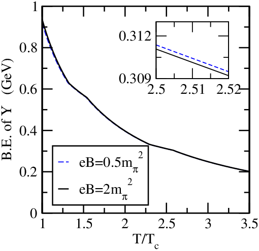
In this subsection, we have obtained the binding energy of and . In order to calculate the binding energy, the real part of the potential Eq.(68) is put into the radial part of the Schrödinger equation, which is then solved numerically to obtain the energy eigenvalues that inturns give the binding energies of quarkonia. To see how the presence of weak magnetic field affects the binding of quarkonia, we have plotted the binding energies of as a function of for different strengths of magnetic field in the left panel of Fig.6. We observed that the binding energy is found to decrease with the temperature and magnetic field both, we can attribute this finding in terms of the increasing of screening with the temperature and magnetic field that we have observed in the real-part of the potential. The point to be noted here is that the difference between the values of binding energies plotted for the magnetic field and is pronounced at higher temperature, this is in accordance with the validity of our work in the weak field limit .
 |
 |
 |
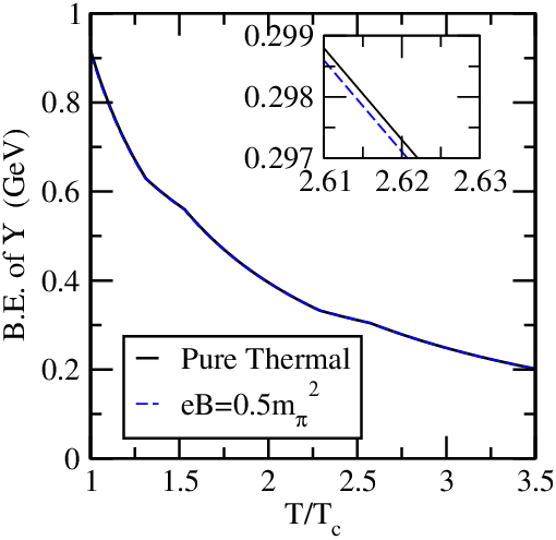 |
In the right panel of Fig.6, we have also compared the binding energy of in presence of weak magnetic field with the pure thermal case. We found that the binding energy in presence of magnetic field is smaller as compared to the one in pure thermal case, this is because the real-part of the potential in presence of magnetic becomes more screened as compared to pure thermal case. The similar observation has also been observed for , except that the value of binding energy for is higher as compared to the value for . The variation of binding energy for is studied in the left and right panel of Fig.7.
4.2 Thermal width
We will now use the imaginary part of the potential obtained in presence of weak magnetic field to estimate the broadening of the resonance states in a thermal medium. So using the first-order time-independent perturbation theory, the width () has been evaluated by folding with (),
| (75) |
the wave function is taken to be the Coloumbic wave function for the ground state
| (76) |
where is the Bohr radius of the heavy quarkonium system. Here we have used the imaginary-part of the potential as a perturbation to obtain the thermal width, and for that purpose we have obtained the imaginary-part of the potential in the small distance limit.
 |
 |
 |
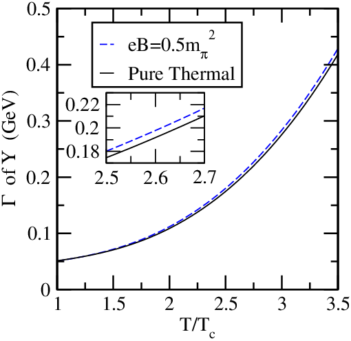 |
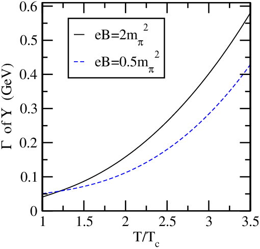
We have obtained the thermal width numerically and observed that it depend on the temperature as well as the weak magnetic field. To explore the effects of the weak magnetic field on the thermal width of heavy quarkonia, we have plotted the thermal width of and as a function of for different strengths of magnetic field in Fig.8 and Fig.9, respectively. We observed that the thermal widths for and get increased both with the temperature and magnetic field as depicted in the left panels of Fig.8 and Fig.9. We can understood this finding in terms of the increase of the imaginary-part of the potential, the magnitude of which gets enhanced both with temperature and magnetic field. We also made a comparison of thermal width in presence of weak magnetic field with its counter part in absence of magnetic field in the right panels of Fig.8 and Fig.9, where we found that the decay widths for and get increased in the presence of magnetic field as compared to the pure thermal case.
4.3 Dissociation of quarkonia
In the previous subsections, we have obtained the binding energies and thermal widths of heavy quarkonia, and . Now we will study the quasi-free dissociation of heavy quarkonia in a thermal QCD medium and see how the dissociation temperatures of quarkonia are affected in the presence of weak magnetic field. For that purpose we use the criterion on the width of the resonance (): [47] (where is the binding energy of the heavy quarkonia) to estimate the dissociation temperature for and .
| Dissociation Temperatures in | ||
|---|---|---|
| State | ||
| Pure Thermal () | 1.80 | 3.50 |
| 1.74 | 3.43 | |
We have obtained the dissociation temperatures of and in the absence and presence of weak magnetic field in Table.1, and observed that the dissociation temperatures become slightly lower in the presence of weak magnetic field. For example, with the and are dissociated at and , respectively whereas with the and are dissociated at and . This observation leads to the slightly early dissociation of heavy quarkonia in the presence of the weak magnetic field.
5 Conclusions
In the present theoretical study, we have explored the effects of weak magnetic field on the dissociation of quarkonia in a thermal QCD by calculating the complex heavy quark potential perturbatively in the aforesaid medium. For that purpose, we first evaluate the gluon self-energy in a similar environment using the imaginary-time formalism. Furthermore, we have revisited the general structure of gluon self-energy tensor in the presence of weak magnetic field in thermal medium and obtained the relevant structure functions, that in turn give rise to the real and imaginary parts of the resummed gluon propagator, which give the real and imaginary parts of the dielectric permittivity. To include the medium modification to the non-perturbative part of the vacuum heavy quark potential, we have included a non-perturbative term in the resummed gluon propagator induced by the dimension two gluon condensate besides the usual hard thermal loop resummed contribution. Thus, the real and imaginary parts of the dielectric permittivity will be used to evaluate the real and imaginary parts of the complex heavy quark potential. We have studied the effects of weak magnetic field on the real and imaginary parts of the potential. We have found that the real-part of the potential is found to be more screened on increasing the value of temperature and magnetic field both. In addition to this, we have observed that the real-part gets slightly more screened in the presence of weak magnetic field as compared to its counter part in the absence of magnetic field. On the other hand, the magnitude of the imaginary-part of the potential gets increased with the value of both temperature and magnetic field, and its magnitude also gets increased in the presence of weak magnetic field as compared to pure thermal case. The real part of the potential is used in the Schrödinger equation to obtain the binding energy of heavy quarkonia, whereas the imaginary part is used to calculate the thermal width. We observed that the binding energies of and are found to decrease with the temperature and magnetic field both, we can attribute this findings in terms of the increasing of screening of the real-part of the potential. We also observed that the binding energy of and in the presence of magnetic field are smaller as compared to the one in the pure thermal case. The increase in the magnitude of the imaginary-part of the potential will leads to the increase of decay width with temperature and magnetic field both. The thermal width for and get increased in presence of magnetic field as compared to pure thermal case. With the observations of binding energy and decay width in hands, we have finally studied the dissociation of quarkonia in the presence of weak magnetic field. The dissociation temperatures for and become slightly lower in the the presence of weak magnetic field. For example, with the and are dissociated at and , respectively whereas with the and are dissociated at and . This observation leads to the slightly early dissociation of quarkonia because of the presence of a weak magnetic field.
Acknowledgements
One of the author BKP is thankful to the CSIR (Grant No.03 (1407)/17/EMR-II), Government of India for the financial assistance. In the following appendices we have shown the explicit calculations of form factors and .
Appendix A Calculation of the form factor
In this appendix, we will use the imaginary-time formalism to calculate the form factor , which is given by
| (77) | |||||
where we have neglected in numerator in the Hard Thermal Loop (HTL) approximation and , the and are given as
| (78) | |||||
| (79) |
Now we substitute , , and , and then perform the frequency sum, which gives as
| (80) | |||||
where the first term is the non-leading term in , thus retaining only the leading term in , the becomes
| (81) |
now taking , which becomes
| (82) | |||||
Substituting and in Eq.(77), the form factor becomes
| (83) |
where we have again resubstituted . Now we will evaluate the real and imaginary parts of the form factor .
The real-part of in the static limit is given by
| (84) | |||||
On the other hand, for the evaluation of the imaginary part of we will us the following identity
| (85) |
along with the following expression
| (86) |
Thus using the above identities Eq.(85) and Eq.(86), the imaginary-part of becomes
| (87) | |||||
which in the static limit takes the simplified form
| (88) |
Appendix B Calculation of the form factor
Similar to the form factor , here we will solve the form factor , which is given by
| (89) | |||||
where we have used the spherical polar coordinate system for . In order to solve the form factor , we will use the method as shown in [38] , which gives
| (90) | |||||
and now we will perform the following frequency sum
| (91) | |||||
Thus, after simplification the form factor becomes
| (92) | |||||
Thus, the real part of in the static limit is obtained as [38]
| (93) |
Now we will evaluate the imaginary part of form factor , for that we write as
| (94) |
where we have defined the following functions:
| (95) | |||||
| (96) | |||||
| (97) | |||||
| (98) |
Now we will evaluate the imaginary parts of all the above four terms one by one using the identities Eq.(85) and Eq.(86), first we start with
where , now the Eq.() in the static limit becomes
where and are the modified Bessel functions of second kind. Now we take
where and the Eq.(), takes the following form in the static limit
Similarly the imaginary part of and
where , and the Eq.() vanishes in the static limit
| (104) |
where , the Eq.() also vanishes in the static limit
| (106) |
Finally, we substitute Eq.(), Eq.(), Eq.(104) and Eq.(106) in Eq.(94), to evaluate the imaginary part of , which in the static limit can be written as
| (107) | |||||
References
- [1] V. Skokov, A. Illarionov, V. Toneev, Int. J. Mod. Phys. A 24, 5925 (2009).
- [2] V. Voronyuk, V. D. Toneev, W. Cassing, E. L. Bratkovskaya, V. P. Konchakovski, S .A. Voloshin, Phys. Rev. C 83, 054911 (2011).
- [3] Kenji Fukushima, Dmitri E. Kharzeev and Harmen J. Warringa, Phys. Rev. D 78, 074033 (2008).
- [4] V. Braguta, M. N. Chernodub, V. A. Goy, K. Landsteiner, A. V. Molochkov and M. I. Polikarpov, Phys. Rev. D 89, 074510 (2014).
- [5] Dmitri E. Kharzeev and Dam T. Son, Phys. Rev. Lett. 106, 062301 (2011).
- [6] V. P. Gusynin, V. A. Miransky and I. A. Shovkovy, Phys. Rev. Lett. 73, 3499 (1994).
- [7] K. Tuchin, Adv. High Energy Phys. 2013, 490495 (2013),
- [8] L. McLerran, V. Skokov, Nucl. Phys. A 929, 184 (2014).
- [9] S. Rath and B. K. Patra, Phys. Rev. D 100, 016009 (2019).
- [10] G.T. Bodwin, E. Braaten, G.P. Lepage, Phys. Rev. D 51, 1125 (1995).
- [11] N. Brambilla, A. Pineda, J. Soto, and A. Vairo, Nucl. Phys. B 566, 275 (2000).
- [12] W. M. Alberico, A. Beraudo, A. De Pace and A. Molinari, Phys. Rev. D 77, 017502 (2008).
- [13] M. Laine, O. Philipsen, and M. Tassler, P. Romatschke, J. High Energy Phys. 03, 054 (2007).
- [14] T. Matsui, H. Satz, Phys. Lett. B 178, 416 (1986).
- [15] A. Beraudo, J. P. Blaizot, C. Ratti, Nucl. Phys. A 806, 312 (2008).
- [16] N. Brambilla, M. A. Escobedo, J. Ghiglieri, A. Vairo, JHEP 1305, 130 (2013).
- [17] L. Thakur, U. Kakade, B. K. Patra, Phys. Rev. D 89, 094020 (2014).
- [18] L. Thakur, N. Haque, U. Kakade, B. K. Patra, Phys. Rev. D 88, 054022 (2013).
- [19] A. Dumitru, Y. Guo, M. Strickland, Phys. Rev. D 79, 114003 (2009).
- [20] B. K. Patra, H. Khanchandani, L. Thakur, Phys Rev D 92, 085034 (2015).
- [21] B. K. Patra, H. Khanchandani, Phys. Rev. D 91, 066008 (2015).
- [22] A. Rothkopf, T. Hatsuda, S. Sasaki, Phys. Rev. Lett. 108, 162001 (2012).
- [23] P. Bagchi, A. M. Srivastava, Mod. Phys. Lett. A 30, 1550162 (2015).
- [24] B. K. Patra, V.J. Menon, Nucl. Phys. A 708, 353 (2002).
- [25] D. Lafferty and A. Rothkopf, arxiv:1906.00035[hep-ph].
- [26] Y. Guo, L. Dong, J. Pan, and M. R. Moldes, Phys. Rev. D 100, 036011 (2019).
- [27] F. Karsch, M. T. Mehr, and H. Satz, Z. Phys. C 37, 617 (1988).
- [28] J. Alford and M. Strickland, Phys. Rev. D 88, 105017 (2013).
- [29] C. Bonati, M. D’Elia, and A. Rucci, Phys. Rev. D 92, 054014 (2015).
- [30] C. Bonati, M. D’Elia, M. Mariti, M. Mesiti, F. Negro, A. Rucci, and F. Sanfilippo, Phys. Rev. D 94, 094007 (2016).
- [31] C. Bonati, M. D’Elia, M. Mariti, M. Mesiti, F. Negro, A. Rucci, and F. Sanfilippo, Phys. Rev. D 95, 074515 (2017).
- [32] K. Fukushima, K. Hattori, H. U. Yee, and Y. Yin, Phys. Rev. D 93, 074028 (2016).
- [33] M. Hasan, B. Chatterjee, B. K. Patra, Eur. Phys. J. C 77, 767 (2017).
- [34] M. Hasan, B. K. Patra, B. Chatterjee, P. Bagchi, Nucl. Phys. A 995, 121688 (2020).
- [35] B. Singh, L. Thakur, H. Mishra, Phys. Rev. D 97, 096011 (2018).
- [36] S. A. Khan, B. K. Patra and M. Hasan, arXiv:2004.08868[hep-ph].
- [37] M. Hasan, B. K. Patra, arXiv:1901.03497[hep-ph].
- [38] B. Karmakar, A. Bandyopadhyay, N. Haque and M. G. Mustafa, Eur. Phys. J. C. 79, 658, (2019).
- [39] B. Singh, S. Mazumder and H. Mishra, arXiv:2002.04922 [hep-ph].
- [40] B. Singh, M. Kurian, S. Mazumder, H. Mishra, V. Chandra and S. K. Das, arXiv:2004.11092[hep-ph].
- [41] A. Ayala, C. A. Dominguez, S. Hernandez-Ortiz, L. A. Hernandez, M. Loewe, D. Manreza Paret and R. Zamora, arXiv:1805.07344v2[hep-ph].
- [42] A. Ayala, C. A. Dominguez, S. Hernandez-Ortiz, L. A.Hernandez, M. Loewe, D. Manreza Paret, and R. Zamora, Phys. Rev. D 98, 031501 (2018).
- [43] H. A. Weldon, Phys. Rev. D 26, 1394 (1982).
- [44] R. D. Pisarski, Phys. Rev. Lett. 63, 1129 (1989).
- [45] E. Shuryak, Zh. Eksp. Teor. Fiz. 74, 408 (1978).
- [46] H. A. Weldon, Phys. Rev. D 42, 2384 (1990).
- [47] A. Mocsy and P. Petreczky, Phys. Rev. Lett. 99, 211602 (2007).