A Sparse Learning Approach to the Detection of Multiple Noise-Like Jammers
Abstract
In this paper, we address the problem of detecting multiple Noise-Like Jammers (NLJs) through a radar system equipped with an array of sensors. To this end, we develop an elegant and systematic framework wherein two architectures are devised to jointly detect an unknown number of NLJs and to estimate their respective angles of arrival. The followed approach relies on the likelihood ratio test in conjunction with a cyclic estimation procedure which incorporates at the design stage a sparsity promoting prior. As a matter of fact, the problem at hand owns an inherent sparse nature which is suitably exploited. This methodological choice is dictated by the fact that, from a mathematical point of view, classical maximum likelihood approach leads to intractable optimization problems (at least to the best of authors’ knowledge) and, hence, a suboptimum approach represents a viable means to solve them. Performance analysis is conducted on simulated data and shows the effectiveness of the proposed architectures in drawing a reliable picture of the electromagnetic threats illuminating the radar system.
Index Terms:
Electronic Counter-Countermeasure, Jamming Detection, Model Order Selection, Noise-Like Jammer, Radar, Signal Classification, Sparse Reconstruction.I Introduction
In the last decades, the radar art has made great strides due to the advances in technology. In fact, the last-generation processing boards are capable of performing huge amounts of computations in a very short time leading to flexible fully-digital architectures. In addition, this abundance of computation power has allowed for the development of radar systems endowed with more and more sophisticated processing schemes. A tangible example is represented by search radars which are primarily concerned with the detection of targets buried in thermal noise, clutter, and, possibly, intentional interference, also known as Electronic Countermeasure (ECM) [1, 2, 3, 4]. In this context, the open literature is continuously enriched with novel contributions that lead to enhanced performances at the price of an increased computational load [5, 6, 7, 8, 9, 10, 11, 12, 13, 14, 15, 16, 17, 18, 19]. Another example related to the potentialities provided by fully-digital architectures is connected with Adaptive Digital BeamForming (ADBF) techniques [4, 2], since they can suitably combine digital samples at the output of each channel according to the specific requirement. Remarkably, by means of ADBF techniques, the transmit/receive antenna beam patterns can be suitably shaped preventing the system engineer from the duplication of hardware resources. For instance, ADBF can be used to build up the auxiliary beam used by the SideLobe Blanker (SLB) [2, 20, 21, 22, 23] exploiting the entire array without the need of additional antennas. The SLB is an Electronic Counter-CounterMeasure (ECCM) against pulsed intentional interferences (or coherent jammers) entering the antenna sidelobes, which, in turn, are ECMs. Note that ECCM techniques can be categorized as antenna-related, transmitter-related, receiver-related, and signal-processing-related depending on the main radar subsystem where they take place [24].
Besides coherent jammers, any radar might also be a victim of noise-like interfering signals, also referred to as Noise-Like Jammers (NLJs), by an adversary force. This electronic attack is aimed at preventing detection or denying accurate measurement of target information (Doppler and/or Range) [4] by generating nondeceptive interference which blends into the thermal noise of the radar receiver. As a consequence, the radar sensitivity is degraded due to the increase of the constant false alarm rate threshold which adapts to the higher level of noise [2, 4]. In addition, this increase makes more difficult to know that jamming is taking place [3, 24]. Under the NLJ attack, the SLB becomes ineffective since it would inhibit the detection of true targets for most of the time. In these situations, the Sidelobe Canceler (SLC) represents a viable ECCM [2, 25, 26]. As a matter of fact, it exploits an additional auxiliary11 1 Note that a system with sidelobe canceling capabilities is equipped with both the main antenna array devoted to target detection and an auxiliary array used to cancel the NLJs. array of antennas (with suitable gains) to adaptively estimate the NLJ Angle of Arrival (AoA) and places nulls in the sidelobes of the main receiver beam along the estimated AoA. In a fully-digital architecture, the task of the SLC can be accomplished by applying ADBF techniques without the use of additional hardware (signal-processing-related ECCM).
However, the application of ADBF techniques might increase the computational burden of the signal processing unit since they require the computation and the inversion of a sample covariance matrix in addition to possible AoA estimation. These operations consume hardware resources which are shared among the different radar functions and, due to the restrictive requirements on radar reaction time, they cannot occur at every dwell regardless whether or not NLJs are illuminating the radar. Thus, it would be highly desirable a preliminary stage capable of detecting NLJs and, possibly, estimating the relevant NLJ parameters. Once the presence of NLJs is declared, the estimated parameters are used by ADBF techniques to contrast the interfering actions. Following this reasoning, in [27], the authors develop a decision scheme which decides for the presence of one NLJ by comparing the spectral properties of reference cells, not affected by jammer returns, with those of Cells Under Test (CUT); no additional information about the NLJ is provided. The case of multiple NLJs is addressed in [28], where the original binary hypothesis test is transformed into a multiple-hypothesis problem and the Model Order Selection (MOS) rules [29, 30, 31, 32, 33, 34] are exploited to conceive two-stage detection architectures, where the first stage provides an estimate of the active NLJs number under the constraint of an upper bound to it, while the second stage is devoted to the detection of the estimated number of NLJs allowing for the control of the false jammer detection probability. However, these two-stage architectures are not capable of providing any information about either the AoA or the received power of the detected NLJs.
With the above remarks in mind, in this paper, we address the same detection problem as in [28] by developing an elegant and systematic framework for the joint detection of multiple NLJs and the estimation of the respective relevant parameters, which include the AoAs and the number of threats22 2 Recall that in [28] the focus is limited to the interference subspace detection [35] without providing any side information.. To this end, we assume that a set of data free of clutter components and affected by thermal noise and possible NLJ components [2, 36, 37] is available at the receiver. As a matter of fact, it can be collected by noticing that the clutter contribution is, in general, range-dependent and tied up to the transmitted waveform. Therefore, it is possible to acquire data free of clutter components and affected by the thermal noise and possible jamming signals only. For instance, for a system employing pulse-to-pulse frequency agility which transmits one pulse, clutter-free data can be collected before transmitting the pulse waveform by listening to the environment (see Figure 1). Another example of practical interest concerns radar systems transmitting coherent pulse trains with a sufficiently high pulse repetition interval. In this case, data collected before transmitting the next pulse and at high ranges (or after the instrumental range), result free of clutter contribution (see Figure 2). Now, under these assumptions, the newly proposed framework exploits a sparse representation of the problem at hand and resorts to suitable cyclic optimization procedures [38] to devise two architectures where the AoA and power estimation is concurrent with the detection without any subsequent estimation stage or constraint on the number of NLJs. Following the lead of [39], we assume that NLJ parameters are random and obey a prior that promotes sparsity. However, the latter is conceived for the specific case at hand giving rise to a new optimization problem and, hence, new analytical derivations. Remarkably, the considered sparsity-based estimation allows for an increase of the angular resolution (at least for high NLJ powers as shown in Section IV). Finally, the obtained estimates are plugged into a Likelihood Ratio Test (LRT) aimed at detecting the presence of NLJs. The above aspects represent the main technical contribution of this work and, at least to the best of authors’ knowledge, appear for the first time in this paper.
It is also important to underline that these methodology choices lead to suboptimum solutions which are dictated by the fact that the plain Maximum Likelihood Approach (MLA) exhibits a difficult mathematical tractability.


Performance analysis, conducted on simulated data, points out the effectiveness of the newly proposed decision schemes from the point of view of both detection and estimation capabilities also in comparison with their natural competitors.
The remainder of the paper is organized as follows. Section II is devoted to problem formulation and definition of quantities used in the next derivations, while the design of the detection architectures and the estimation procedures are described in Section III. Section IV shows the effectiveness of the proposed strategies through numerical examples on simulated data. Finally, Section V contains concluding remarks and charts a course for future works; some mathematical derivations and proofs are confined to the appendices.
I-A Notation
In the sequel, vectors and matrices are denoted by boldface lower-case and upper-case letters, respectively. The th entry of a vector is represented by whereas symbols , , , and denote the determinant, trace, transpose, and conjugate transpose, respectively. Symbol denotes the Euclidean norm of a vector. As to numerical sets, is the set of natural numbers, is the set of real numbers, is the Euclidean space of -dimensional real matrices (or vectors if ), is the set of -dimensional real matrices (or vectors if ) whose entries are greater than or equal to zero, is the set of complex numbers, and is the Euclidean space of -dimensional complex matrices (or vectors if ). The modulus of a real number is denoted by . and stand for the identity matrix and the null vector or matrix of proper size. Symbol means that the left-hand side is proportional to the right-hand side. Given a vector , indicates the diagonal matrix whose th diagonal element is the th entry of . The acronym pdf stands for probability density function and the conditional pdf of a random variable given another random variable is denoted by . Finally, we write if is a complex circular -dimensional normal vector with mean and positive definite covariance matrix .
II Problem Formulation and Preliminary Definitions
Consider a radar system equipped with spatial channels which is listening to the environment. The incoming signal is firstly conditioned by means of a baseband down-conversion, then, it is pre-processed and properly sampled. The samples are, then, organized to form -dimensional vectors denoted by , , with being the total number of listening data and the number of NLJs. The detection problem at hand can be formulated as
| (1) |
where and
| (2) |
In the last equations, and33 3 As explained in Appendix A, the lower bound on the thermal noise power is required to ensure a good behavior for the prior associated to that will be introduced in the next section. From a practical point of view, this lower bound can be handled by exploiting a suitable numerical representation used by the signal processing unit. are the powers of thermal noise and the th jammer, respectively, is the AoA of the th jammer measured with respect to the array broadside, and is the array steering vector pointed along whose expression is with the array interelement spacing and the carrier wavelength. Moreover, under each hypothesis, s are statistically independent.
In order to bring to light the sparse nature of the problem, let us sample the angular sector under surveillance to form a discrete and finite set of angles denoted by with and . In addition, we assume that , . Thus, if we define a vector such that
| (3) |
it follows that is sparse (since ) and the ICM under can be recast as
| (4) |
where is the dictionary and . In Figure 3, we show a pictorial representation of the hidden sparse nature of (2). Thus, the formal structure of the detection problem at hand can be expressed in terms of the sparse vector as follows
| (5) |
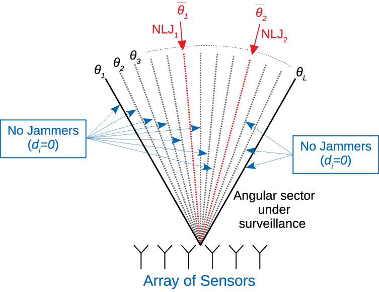
Finally, we conclude this section by providing the expression of the pdf of under , , which will be used in the next developments, namely
| (6) |
III Architecture Designs
As stated in Section I, the MLA for this problem leads to intractable mathematics and, hence, we resort to a suboptimum iterative approach. With this remark in mind, in this section, we derive two decision schemes for problem (5) which differ in the adaptivity with respect to the thermal noise power. Specifically, the former estimates assuming that is known and, then, replaces it with an estimate which is assumed available at the receiver (a point better explained in the next subsection). The latter jointly estimates and by means of a cyclic optimization procedure. In both cases, the structure of the decision statistic is given by the likelihood ratio and the decision rule is given by the LRT, whose expression is
| (7) |
where is threshold44 4 Hereafter, we denote by any modification of the detection threshold. to be set in order to guarantee the required Probability of False Jammer Detection ().
III-A Adaptive detector for unknown
Let us assume that is known and, following the lead of [39], that the entries of are jointly distributed according to a sparsity promoting (possibly improper) prior given by55 5 There does not exist a specific criterion to select the prior for the considered framework. Nevertheless, the choice of this prior raises from an analysis of the achievable performance.
| (8) |
with a (possible) positive constant of proportionality, where is a parameter allowing for sparsity control. In Appendix A, we investigate the behavior of with respect to and . Thus, the logarithm of the joint pdf of and under can be written as
| (9) |
where and proportionality constant of the prior of has been neglected. Now, we proceed by setting to zero the first derivative of with respect to [35], namely , , which leads to the following equations
| (10) |
Observe that when or , then and, hence, the following matrix
| (11) |
is positive definite. Equations (10) can be written in matrix form as
| (12) |
with and is used to guarantee the constraint that the entries of are nonnegative. Now, given a preassigned value for , let us assume that an initial estimate of , denoted by , is available, then, it is possible to apply a cyclic optimization [39, 38] whose th step is given by
| (13) |
It is important to highlight that the described procedure leads to a nondecreasing sequence of values for the cost function , . As a matter of fact, first note that is continuous and
| (14) |
The above conditions imply that is upper bounded over . Moreover, exploiting Lemma 1 and Theorem 2 of [39] it is not difficult to show that
| (15) |
It still remains to estimate . To this end, let us sample to come up with a finite set of admissible values for denoted by . Now, given and the maximum number of jammers , let us denote the number of peaks by (), in as follows
- 1.
sort the entries of from the largest to the smallest and form vector ;
- 2.
select returning the lowest value of
(16) with66 6 Note that (16) is reminiscent of the Minimum Description Length criterion applied in [34]. and being computed as described in Appendix B (and summarized in Algorithm 1), where an alternating optimization procedure is applied by setting to zero the entries of whose indices are different from those of computed with respect to the element indices of .
As a result, we obtain the set and the estimate of is obtained as
| (17) |
Finally, several stopping criteria can be thought to interrupt the cycles. For instance, they can rely on a maximum number of iterations or on the relative variations with respect to the values returned at the previous iteration. The entire procedure is outlined in Algorithm 2.
Gathering the above estimates, the adaptive LRT can be written as
| (18) |
where and is an estimate of the thermal noise power available at the receiver. For instance, the value of such estimate can be an entry of a Lookup Table accounting for different system operating conditions or alternatively, it can be periodically computed according to the plan of the system scheduler by disabling the antenna front-end. Architecture (18) will be referred to in the following as Sparse Cyclic LRT (SC-LRT). In the next subsection, we conceive an adaptive procedure which exploits data under test to jointly estimate and at the price of an additional computational burden. As a matter of fact, such new procedure comprises two steps which are iterated until a stopping criterion is satisfied. Specifically, the first step is described in the present subsection, whereas the second step will be devised in what follows. Thus, the additional computational load is due to both the second step and the required iterations.
III-B Adaptive detector for unknown and
In this case, both and must be estimated from data. While the Maximum Likelihood Estimate (MLE) of under can be obtained in closed-form, the estimation of the unknown parameters under is more problematic and requires elaborate approaches. To this end, let us note that the estimation procedure for described in the previous subsection, which assumes that is known, can be viewed as a step of a cyclic procedure that, when is unknown, repeats the following operations
- 1.
assume that is known and estimate ;
- 2.
assume that is known and estimate .
Moreover, the estimates obtained at the previous iteration replace the quantities assumed known at the current iteration and so on. Since the first step of this procedure is described in Subsection III-A, we complete here the procedure by describing the missing part, namely the estimation of .
Thus, let us start assuming that is in force and that an estimate of at the th iteration, say, is available. Then, compute the MLE of for , which is tantamount to solving
| (19) |
where is the log-likelihood function for . Now, note that the is a continuous function such that
| (20) |
As a consequence, the maximum of occurs at either or the local stationary points. In this case, it can be found by setting to zero the first derivative of with respect to , namely
| (21) |
where is a diagonal matrix whose nonzero entries are the eigenvalues of denoted by with , whereas with a unitary matrix whose columns are the eigenvectors of corresponding to , . Now, by Abel-Ruffini Theorem [40], when , equation (21) does not admit solutions in algebraic form. For this reason, we solve it resorting to numerical routines and choose the positive solution, say, greater than or equal to and that returns the highest value of . If such solution does not exist, we set . Once is available, we exploit the cyclic optimization of Subsection III-A to compute where is replaced by . The entire procedure, summarized in Algorithm 3, can terminate after a fixed number of iterations or when a convergence criterion is satisfied as, for instance,
| (22) |
with a suitable small positive number.
On the other hand, under , it is not difficult to show that the MLE of is given by
| (23) |
and replacing the above estimates in the LRT, we come up with
| (24) |
where and are the final estimates provided by Algorithm 3. In what follows, we refer to the above decision scheme as Sparse Doubly Cyclic LRT (SDC-LRT).
Before concluding this section and presenting the numerical examples, we highlight that the estimate of , say, can be used to infer the number of NLJs and their AOAs. However, may contain false objects (ghosts) induced by the energy spillover. In order to mitigate the number of ghosts, we apply an additional thresholding of the entries of and we resort to the same fusion strategy proposed in [41], where the grid used to sample the angular sector under surveillance is partitioned into subsets associated to a specific AOA and the entries of falling in a subset are merged together. The interested reader is referred to [41] for further details. Finally, it is clear that other fusion strategies are possible leading to better estimation and/or classification performance especially in the case where the actual AOAs of the NLJs are in between the points of the sampling grid. For instance, an interpolation of consecutive nonzero entries of can be performed, whereupon the resulting peaks can be selected. Another approach would consist in increasing the angular resolution of the grid in the sectors that contain consecutive nonzero entries of . As a result, the actual AOAs of the NLJs are very close to the oversampled grid points. The design of different fusion strategies is out of the scope of the present paper and represents the current research line.
IV Illustrative Examples and Discussion
In this section, we present some numerical examples aimed at showing the detection and estimation capabilities of the SDC-LRT and the SC-LRT for known77 7 Comparing SC-LRT for known with the SDC-LRT allows us to quantify the loss due to the estimation of . . For comparison purpose, we also assess the performance of the LRT where the unknown parameters are estimated by means of the SParse Iterative Covariance-based Estimation (SPICE) algorithm whose theoretical formulation is laid down in [42] and that is well-suited to the covariance matrix model at hand given by (4). This competitor will be denoted by the acronym SPICE-LRT. Two operating scenarios are considered, which differ in the number of NLJs. Specifically, the former contains NLJs, whereas the latter is characterized by the presence of NLJs. In both scenarios, NLJs share the same (nominal) power and are located within an angular sector under surveillance ranging from to and uniformly sampled at degree, degrees, or degrees. The nominal AOA of the NLJs, measured with respect to the array normal, are assumed to lie on the sampling grid (“on-grid” case) and are given by
- •
and for a spatial sampling rate of degree, degree, and degree in the scenario which assumes NLJs;
- •
, , and for a spatial sampling rate of degree, degree, and degree in the other scenario which assumes NLJs.
Besides, we also consider the “off-grid” situation where the actual AOAs of the NLJs are in between the grid samples (a point better explained below). Finally, we show that at high NLJ power, the proposed algorithms provide high-quality estimates of the NLJ parameters.
The Jammer-to-Noise Ratio (JNR) is defined as with . The analysis relies on the following figures of merit:
- •
the Probability of Jammer Detection () for a given ;
- •
the Root Mean Square (RMS) value for the number of missed NLJs, the number of ghost NLJs and the Hausdorff metric [43] between88 8 Note that such figures of merit make sense when the performance are evaluated on-grid assumption. Conversely, in the case of off-grid angular positions, another figure of merit must be considered. and . The latter belongs to the family of the multi-object distances which are able to capture the error between two sets of vectors and is defined as with and are the sets of the coordinates of the nonzero entries of and , respectively (these figures of merit are computed exploiting the fusion strategy of [41] with a subset cardinality equal to );
- •
the classification histograms (computed exploiting the fusion strategy of [41] with a subset cardinality equal to ) namely the percentages of declaring that , , NLJs are present when the actual number of NLJs is either or ;
- •
the RMS values for the angular error between the actual AOA and the estimated direction closest to the former (off-grid case only).
Due to the lack of closed-form expressions for the above metrics, we resort to standard Monte Carlo counting techniques. Specifically, the detection thresholds are computed over independent trials with , whereas the classification percentages and the RMS values are estimated exploiting independent trials. In the case of off-grid NLJ angular positions, at each Monte Carlo trial, the AOAs are generated as independent random variables uniformly distributed in or degrees, or , where is the grid sampling interval. It is worth noticing that this off-grid analysis is aimed at illustrating the behavior of the newly proposed method in three different situations, namely an unfavorable case where the grid is sampled at degree (and, hence, the variation range of the actual direction for each jammer comprises three grid points), a favorable case where the grid is sampled at degrees (i.e., the actual direction of each jammer is very close to a nominal grid point), and an intermediate situation with a sampling interval of degrees. From an operating point of view, it would be possible to bring back to one of the above cases by oversampling the angular sectors identified by a preliminary application of the estimation procedure over a rough search grid. Moreover, as already stated, we perform an additional thresholding of the entries of . To this end, the threshold is set to ensure a probability of declaring the presence of spurious NLJs equal to . Finally, all the numerical examples assume and , whereas the estimation procedures terminate when the convergence criterion in (22) is satisfied with .
IV-A First Operating Scenario: NLJs
Let us start the analysis by focusing on the scenario that contains NLJs. In Figure 4, we plot the of the decision schemes devised in Subsections III-A and III-B along with that of the SPICE-LRT assuming that the AOAs of the NLJs belong to the sampling grid. Inspection of the figure highlights that the performance improves as the sampling interval grows. This behavior can be motivated by noticing that a wider sampling interval would decrease the coherence of the dictionary leading, as a consequence, to an improvement of the estimation quality of [44]. Moreover, the proposed detectors exhibit a gain of about dB at with respect to the SPICE-LRT. It is also worth observing that the for SC-LRT and SDC-LRT achieves values greater than for JNR values greater than about dB.
In Figure 5, the RMS values for the Hausdorff distance between the true and estimated , the number of missed jammers, and the number of ghosts against the JNR are plotted for the same parameter values as in Figure 4. Both the SPICE and the proposed procedure (Algorithm 3) exhibit excellent performance rates which improve as the JNR increases. However, to be more precise, the proposed procedure performs slightly better than SPICE for the considered figures of merit and the parameter setting. As a matter of fact, for high JNR values the Hausdorff distance provided by SPICE is biased whereas that related to the proposed procedure is strictly decreasing as the JNR increases. The differences observed in the last two subfigures are less evident except for the RMS number of ghosts when the grid is sampled at degree. In order to provide a complete picture of the performance for the on-grid case comprising NLJs, Figure 6 shows the classification histograms assuming dB (recall that NLJs transmit very high power) and the nominal AOA for the NLJs. More precisely, such histograms count the number of times that the estimation procedures state that NLJs are present (recall that the ground-truth is NLJs). It turns out that the proposed procedure can guarantee a percentage of correct estimation for the number of NLJs greater than % for all the considered sampling intervals, whereas SPICE exhibits percentage higher than % when the grid sampling rate is or degrees. For the case of a grid sampled at degree, the percentage of correct estimation for SPICE decreases to about % yielding a nonnegligible overestimation attitude.
The next illustrative example assumes that the NLJs have not yet transmitted their maximum power level when the radar is forming the set of data under test. Specifically, for each nominal JNR value, we generate with a JNR given by the nominal value minus dB, then the remaining s, , are built up increasing the initial JNR by dB until the nominal value is achieved. Figure 7, where the is shown as a function of the JNR for this scenario, confirms the ranking observed in Figure 4 with a slight performance degradation, which is, nevertheless, expected since the actual amount of collected energy is less than the nominal value. As for the other figures of merit, results not reported here for brevity are aligned with what observed in Figures 5 and 6.
Now, we focus on the case where the actual angular positions of the three NLJs are in between the grid points. In this case, besides the detection performance, we consider the classification histograms and RMS value of the angular difference between the actual position of the NLJs and estimated direction which is closest to the former. Note that the other figures of merit do not make sense in this case. The detection performance is shown in Figure 8 where an overall loss of at most dB at and for the curves related to the sampling intervals of and degrees can be measured with respect to Figure 4. On the other hand, the curves representative of the grid sampled at degree remain unaltered. The figure also confirms that the SC-LRT and SDC-LRT are superior to the SPICE-LRT with a gain of about dB and, in addition, that a wider sampling interval leads to slightly better performance. The classification histograms under the off-grid assumption are shown in Figure 9, where, as expected, a sampling interval of degrees enhances the estimation quality for the number of NLJs since it decreases the energy spillover of the NLJs between consecutive grid points. In this case, the proposed procedure is slightly superior to the SPICE algorithm. For a sampling interval of and degrees, both algorithms provide a percentage of correct classification less than % with the SPICE algorithm being more inclined to overestimate the number of NLJs than the proposed procedure. For instance, note that for a sampling interval of degree, the sum of the occurrences for the SPICE is less than , because the latter in some Monte Carlo trials returns a number of NLJs greater than . In the Figure 10, we plot the RMS angular distance between the actual AOA and the estimated AOA closest to the former versus the JNR. The figure points out that the considered procedures share the same performance and, more precisely, for JNR values greater than dB the RMS error is less than degrees. Importantly, a grid sampled at degrees allows for RMS values less than degree for JNR dB. Finally, in Figures 11-12, we compute the detection curves and the classification histograms by assuming that the actual NLJ angular positions are uniformly distributed in a window centered on the nominal AoA and of size exactly equal to the sampling interval. The behavior observed in these last figures is aligned with that described before confirming the superiority of the proposed method over SPICE.
The last illustrative example (Figure 13) of this subsection shows that the estimation quality is high in the case of large NLJ power values. To this end, we show the returned estimates for two outcomes of two Monte Carlo trials. Specifically, in Subplot (a), we plot the interference power estimates as a function of the angles belonging to the search grid sampled at degree for three jammers at , , and with JNR= dB; Subplot (b) shares the same parameter setting as Subplot (a) but for the NLJ AoAs, which are , , and . Inspection of Subplot (a) highlights the enhanced resolution provided by the sparse approach along with a significant attenuation of “sidelobe” effects, whereas in Subplot (b), the spillover of the NLJ power between adjacent grid points can be observed motivating the need of suitable fusion strategies.


IV-B Second Operating Scenario: NLJs
In this last subsection, we repeat previous analysis assuming that NLJs are present. This analysis is aimed at investigating the effect of an increase of the NLJ number on the performance.
The detection performance is shown in Figure 14, that clearly confirms the hierarchy observed in Figure 4 with the SC-LRT and SDC-LRT achieving better results than the SPICE-LRT. Moreover, the presence of an additional NLJ increases the overall JNR and, hence, the detection performance. Figures 15-16 are related to the classification/estimation performance for the on-grid case and share the same parameters as Figures 5-6 except for . From the comparisons with respect to the first operating scenario, it stems that the estimation performance is preserved when the number of NLJs changes from to . In the last two figures, we plot the classification histograms as well as the RMS values of the error between the actual AOA and the estimated AOA closest to the former. The histograms, reported in Figure 17, show that the SPICE is again more inclined than the proposed procedure to overestimate the number of NLJs especially for a sampling interval of degree (note that also in this case the sum of the occurrences returned by SPICE is less than , since it may estimate a number of jammers greater than ). Finally, the comments related to Figure 10 also hold for Figure 18.


V Conclusions
In this paper, we have proposed signal-processing-based radar solutions for the adaptive detection of multiple NLJs. Specifically, such decision schemes are capable to estimate the number of NLJs illuminating the radar system and to return their respective AoAs. As a result, the system can draw a picture of the electromagnetic threats which are active in the radar operating scenario. From the design point of view, since the plain MLA leads to intractable optimization problems from a mathematical point of view (at least to the best of authors’ knowledge), we resorted to a suboptimum approach by developing a systematic framework which relies on cyclic optimizations and accounts for a sparsity promoting prior at the design stage due to the inherent sparse nature of the problem. In this context, two adaptive architectures have been devised and assessed using simulated data. Specifically, the analysis has highlighted that such architectures can provide reliable detection and estimation performance outperforming their competitor at least for the considered parameter setting. Future research tracks might include the design of enhanced fusion strategies aimed at handling the artifacts and improving the grid resolution or the extension of the above framework to the case of multiple coherent targets. The former issue is part of the current research line. Finally, another research line is related to the application of this approach to the new 5G context where phased arrays are exploited [45].
Acknowledgements
This work has been partially supported by NSF under grants No. 1708509 and No. 61971412, as well as by the EU research project LOCUS No. 871249.
Appendix A Properties of the sparsity-promoting prior
In this appendix, we describe the properties of defined by (8) in order to show that, through , it is possible to tune its behavior in terms of sparsity promotion. For simplicity, in what follows we neglect the normalization constant. It is also important to remark that is a suitable modification of the prior introduced in [39] for the specific problem at hand (see also the footnote in Section 2).
Let us start by noticing that, given , is continuous and
| (25) | ||||
| (26) |
where the last equality can be proved by defining , where is the th vector of the standard basis of , and rewriting the numerator of (8) (neglecting, for simplicity, its power) as follows
| (27) | ||||
| (28) |
where the third equality comes from the application of the Woodbury identity [46] and the last inequality is due to the fact that is positive semidefinite. Iterating the above line of reasoning to and so on by considering , , and , yields the following inequality
| (29) |
which allows to apply the Squeeze Theorem [47] and (26) follows. The above proof also shows that
| (30) |
As for the monotonicity of with respect to the generic , observe that
| (31) |
and let us study the sign of the first derivative of , whose expression is
| (32) |
with . Since the denominator of the above equation is always positive, we focus on the numerator, which can be recast as
| (33) |
Now, when , it turns out that and hence is strictly decreasing. This behavior is also observed when and . In the case where , there exists a local stationary point in the interval (0, 1). However, the lower bound on guarantees that and that the prior is more oriented to sparsity avoiding the local stationary point between and .
Finally, we consider the limit case , which implies that
| (34) |
where we have used the following well-known result . It is straightforward to show that . On the other hand, the limit for large can be computed exploiting (27), which leads to the following inequality
| (35) |
Using the above equation in conjunction with the Squeeze Theorem, we come up with . As the last remark, it is not difficult to show that
| (36) |
and, hence, that is strictly decreasing with respect to the generic .
Appendix B Cyclic optimization to compute
Let us consider a preassigned value of and denote by the vector of integers representing the indices of the elements of with respect to (recall that the former is an ordered copy of the latter). Now, we form a vector such that
| (37) |
namely, the entries of , that do not correspond to the selected peaks, are set to zero. Assume that an estimate at the th iteration of the procedure in question is available, then, starting from the logarithm of the pdf of under (namely, the logarithm of (6) under ), , we can define the following function to be optimized
| (38) |
where with and . Note that is positive definite and can be decomposed as . Thus, applying the Woodbury identity [48] and the equality
| (39) |
where and , equation (38) becomes
| (38) | ||||
| (40) |
Setting to zero the first derivative of with respect to leads to the following equation
| (41) | ||||
| (42) | ||||
| (43) | ||||
| (44) |
Thus, initializing the procedure with obtained using and , we can estimate through the following update rule
| (45) |
Before concluding this appendix an important remark on the convergence of the procedure is in order. Specifically, observe that is continuous, increasing when , decreasing when , and
| (46) |
It follows that there exists a unique global maximum of with respect to and the iterative procedure gives rise to the following increasing sequence
| (47) |
where
| (48) |
In order to prove (47), let us note that, by construction, the following inequalities hold
| (49) |
Now, observe that since the function
| (50) |
is continuous and such that
| (51) |
namely is upper bounded, sequence (47) does not diverge. The cyclic optimization, sketched in Algorithm 1, terminates according to a suitable stopping condition based upon the maximum number of iterations or the estimate variations with respect to the values at the previous iteration.
References
- [1] M. A. Richards, J. A. Scheer, and W. A. Holm, Principles of Modern Radar: Basic Principles. Raleigh, NC: Scitech Publishing, 2010.
- [2] A. Farina, Antenna-Based Signal Processing Techniques for Radar Systems. Boston, MA: Artech House, 1992.
- [3] D. Adamy, EW101: A First Course in Electronic Warfare. Norwood, MA: Artech House, 2001.
- [4] W. L. Melvin and J. A. Scheer, Principles of Modern Radar: Advanced Techniques, S. Publishing, Ed., Edison, NJ, 2013.
- [5] E. J. Kelly, “An adaptive detection algorithm,” IEEE Transactions on Aerospace and Electronic Systems, no. 2, pp. 115–127, 1986.
- [6] F. C. Robey, D. R. Fuhrmann, E. J. Kelly, and R. Nitzberg, “A CFAR adaptive matched filter detector,” IEEE Transactions on Aerospace and Electronic Systems, vol. 28, no. 1, pp. 208–216, 1992.
- [7] F. Gini and A. Farina, “Vector Subspace Detection in Compound-Gaussian Clutter Part I: Survey and New Results,” IEEE Transactions on Aerospace and Electronic Systems, vol. 38, no. 4, pp. 1295–1311, 2002.
- [8] D. Orlando and G. Ricci, “A Rao Test With Enhanced Selectivity Properties in Homogeneous Scenarios,” IEEE Transactions on Signal Processing, vol. 58, no. 10, pp. 5385–5390, 2010.
- [9] W. Liu, W. Xie, and Y. Wang, “Rao and Wald Tests for Distributed Targets Detection With Unknown Signal Steering,” IEEE Signal Processing Letters, vol. 20, no. 11, pp. 1086–1089, 2013.
- [10] Y. I. Abramovich and B. A. Johnson, “GLRT-based detection-estimation for undersampled training conditions,” IEEE Transactions on Signal Processing, vol. 56, no. 8, pp. 3600–3612, 2008.
- [11] F. Bandiera, D. Orlando, and G. Ricci, Advanced Radar Detection Schemes Under Mismatched Signal Models. San Rafael, US: Synthesis Lectures on Signal Processing No. 8, Morgan & Claypool Publishers, 2009.
- [12] J. Liu, H. Li, and B. Himed, “Persymmetric adaptive target detection with distributed MIMO radar,” IEEE Transactions on Aerospace and Electronic Systems, vol. 51, no. 1, pp. 372–382, 2015.
- [13] J. Liu, G. Cui, H. Li, and B. Himed, “On the performance of a persymmetric adaptive matched filter,” IEEE Transactions on Aerospace and Electronic Systems, vol. 51, no. 4, pp. 2605–2614, 2015.
- [14] J. Liu, S. Sun, and W. Liu, “One-step persymmetric GLRT for subspace signals,” IEEE Transaction on Signal Processing, vol. 14, no. 67, pp. 3639–3648, July 15 2019.
- [15] C. Hao, S. Gazor, G. Foglia, B. Liu, and C. Hou, “Persymmetric adaptive detection and range estimation of a small target,” IEEE Transactions on Aerospace and Electronic Systems, vol. 51, no. 4, pp. 2590–2604, 2015.
- [16] A. De Maio and D. Orlando, “An Invariant Approach to Adaptive Radar Detection Under Covariance Persymmetry,” IEEE Transactions on Signal Processing, vol. 63, no. 5, pp. 1297–1309, 2015.
- [17] A. De Maio, D. Orlando, C. Hao, and G. Foglia, “Adaptive Detection of Point-like Targets in Spectrally Symmetric Interference,” IEEE Transactions on Signal Processing, vol. 64, no. 12, pp. 3207–3220, 2016.
- [18] G. Foglia, C. Hao, A. Farina, G. Giunta, D. Orlando, and C. Hou, “Adaptive Detection of Point-Like Targets in Partially Homogeneous Clutter With Symmetric Spectrum,” IEEE Transactions on Aerospace and Electronic Systems, vol. 53, no. 4, pp. 2110–2119, 2017.
- [19] C. Hao, D. Orlando, G. Foglia, and G. Giunta, “Knowledge-Based Adaptive Detection: Joint Exploitation of Clutter and System Symmetry Properties,” IEEE Signal Processing Letters, vol. 23, no. 10, pp. 1489–1493, October 2016.
- [20] A. Farina and F. Gini, “Calculation of Blanking Probability for the Sidelobe Blanking for Two Interference Statistical Models,” IEEE Signal Processing Letters, vol. 5, no. 4, pp. 98–100, April 1998.
- [21] A. De Maio, A. Farina, and F. Gini, “Performance Analysis of the Sidelobe Blanking System for Two Fluctuating Jammer Models,” IEEE Transactions on Aerospace and Electronic Systems, vol. 41, no. 3, pp. 1082–1091, July 2005.
- [22] G. Cui, A. De Maio, A. Aubry, A. Farina, and L. Kong, “Advanced SLB Architectures with Invariant Receivers,” IEEE Transactions on Aerospace and Electronic Systems, vol. 49, no. 2, pp. 798–818, April 2013.
- [23] G. Cui, A. De Maio, M. Piezzo, and A. Farina, “Sidelobe Blanking with Generalized Swerling-Chi Fluctuation Models,” IEEE Transactions on Aerospace and Electronic Systems, vol. 49, no. 2, pp. 982–1005, April 2013.
- [24] A. Farina, “Eccm techniques,” in Radar Handbook, M. I. Skolnik, Ed. McGraw-Hill, 2008, ch. 24.
- [25] ——, “Single Sidelobe Canceller: Theory and Evaluation,” IEEE Transactions on Aerospace and Electronic Systems, vol. 13, no. 6, pp. 690–699, November 1977.
- [26] E. J. Hendon and I. S. Reed, “A new CFAR sidelobe canceler algorithm for radar,” IEEE Transactions on Aerospace and Electronic Systems, vol. 26, no. 5, pp. 792–803, September 1990.
- [27] D. Orlando, “A Novel Noise Jamming Detection Algorithm for Radar Applications,” IEEE Signal Processing Letters, vol. 24, no. 2, pp. 206–210, Feb 2017.
- [28] V. Carotenuto, C. Hao, D. Orlando, A. De Maio, and S. Iommelli, “Detection of Multiple Noise-like Jammers for Radar Applications,” in 2018 5th IEEE International Workshop on Metrology for AeroSpace (MetroAeroSpace), June 2018, pp. 328–333.
- [29] P. Stoica and P. Babu, “On the Exponentially Embedded Family (EEF) Rule for Model Order Selection,” IEEE Signal Processing Letters, vol. 19, no. 9, pp. 551–554, September 2012.
- [30] P. Stoica and Y. Selen, “Model-order selection: A review of information criterion rules,” IEEE Signal Processing Magazine, vol. 21, no. 4, pp. 36–47, 2004.
- [31] S. M. Kay, A. H. Nuttall, and P. M. Baggenstoss, “Multidimensional probability density function approximations for detection, classification, and model order selection,” IEEE Transactions on Signal Processing, vol. 49, no. 10, pp. 2240–2252, October 2001.
- [32] S. Kay, “Conditional model order estimation,” IEEE Transactions on Signal Processing, vol. 49, no. 9, pp. 1910–1917, September 2001.
- [33] S. M. Kay, “The Multifamily Likelihood Ratio Test for Multiple Signal Model Detection,” IEEE Signal Processing Letters, vol. 12, no. 5, pp. 369–371, 2005.
- [34] M. Wax and T. Kailath, “Detection of signals by information theoretic criteria,” IEEE Transactions on Acoustics, Speech, and Signal Processing, vol. 33, no. 2, pp. 387–392, 1985.
- [35] H. L. Van Trees, Optimum Array Processing (Detection, Estimation, and Modulation Theory, Part IV). John Wiley & Sons, 2002.
- [36] J. Ward, “Space-time adaptive processing for airborne radar,” MIT Lincoln Laboratory, Tech. Rep., 1994.
- [37] V. Carotenuto, A. De Maio, D. Orlando, and L. Pallotta, “Adaptive Radar Detection Using Two Sets of Training Data,” IEEE Transactions on Signal Processing, 2017, in early access.
- [38] P. Stoica and Y. Selen, “Cyclic minimizers, majorization techniques, and the expectation-maximization algorithm: a refresher,” IEEE Signal Processing Magazine, vol. 21, no. 1, pp. 112–114, 2004.
- [39] X. Tan, W. Roberts, J. Li, and P. Stoica, “Sparse Learning via Iterative Minimization With Application to MIMO Radar Imaging,” IEEE Transactions on Signal Processing, vol. 59, no. 3, pp. 1088–1101, March 2011.
- [40] P. Pesic, Abel’s Proof: An Essay on the Sources and Meaning of Mathematical Unsolvability, ser. The MIT Press. MIT Press, 2004.
- [41] L. Yan, P. Addabbo, C. Hao, D. Orlando, and A. Farina, “New ECCM Techniques Against Noise-like and/or Coherent Interferers,” IEEE Transactions on Aerospace and Electronic Systems, 2019.
- [42] P. Stoica, P. Babu, and J. Li, “SPICE: A Sparse Covariance-Based Estimation Method for Array Processing,” IEEE Transactions on Signal Processing, vol. 59, no. 2, pp. 629–638, Feb 2011.
- [43] D. Schuhmacher, B. Vo, and B. Vo, “A Consistent Metric for Performance Evaluation of Multi-Object Filters,” IEEE Transactions on Signal Processing, vol. 56, no. 8, pp. 3447–3457, 2008.
- [44] E. J. Candes and M. B. Wakin, “An introduction to compressive sampling,” IEEE Signal Processing Magazine, vol. 25, no. 2, pp. 21–30, March 2008.
- [45] “3GPP TR 33.809 V0.8.0,” 3rd Generation Partnership Project, Tech. Rep., November 2019. [Online]. Available: https://portal.3gpp.org/desktopmodules/Specifications/SpecificationDetails.aspx?specificationId=3539
- [46] R. A. Horn and C. R. Johnson, Matrix Analysis, C. U. Press, Ed., 1985.
- [47] H. Sohrab, Basic Real Analysis. Springer New York, 2014.
- [48] G. Golub and C. Van Loan, Matrix Computations, ser. Johns Hopkins Studies in the Mathematical Sciences. Johns Hopkins University Press, 1996.
![[Uncaptioned image]](2004.12677v1/yan.png) |
Linjie Yan Linjie Yanreceived the B.E. degree in communication engineering from Shandong University of Science and Technology, Shandong, China, in 2016. She is currently working toward the Ph.D. degree in signal and information processing at the Institute of Acoustics,Chinese Academy of Sciences, Beijing, China. |
![[Uncaptioned image]](2004.12677v1/addabbo.png) |
Pia Addabbo Pia Addabbo received the B.Sc. and M.Sc. degrees in telecommunication engineering, and the Ph.D. degree in information engineering from the Universit degli Studi del Sannio, Benevento, Italy, in 2005, 2008, and 2012, respectively.,She is a Researcher at the “Giustino Fortunato” University, Benevento, Italy. Her research interests include statistical signal processing applied to radar target recognition, global navigation satellite system reflectometry, and hyperspectral unmixing.,Dr. Addabbo is a member of IEEE from 2009 and coauthor of scientific publications in international journals and conferences. |
![[Uncaptioned image]](2004.12677v1/zhang.png) |
Yuxuan Zhang Yuxuan Zhang received the B.E. degree in electronic and information engineering from Harbin Engineering University, Heilongjiang, China, in 2018. He is now studying for the master degree in signal and information processing in Institute of Acoustics, Chinese Academy of Sciences, Beijing, China. |
![[Uncaptioned image]](2004.12677v1/hao.png) |
Hao Chengpeng Chengpeng Hao(M’08–SM’15) received the B.S. and M.S. degrees in electronic engineering from Beijing Broadcasting Institute, Beijing, China, in 1998 and 2001 respectively,and the Ph.D. degree in signal and information processing from the Institute of Acoustics,Chinese Academy of Sciences, Beijing, China, in 2004.He is currently a Professor with the State Key Laboratory of Information Technology for Autonomous Underwater Vehicles, Chinese Academy of Sciences. He has held a visiting position with the Electrical and Computer Engineering Department, Queens University, Kingston, ON, Canada from July 2013 to July 2014. He authored or coauthored more than 100 journal and conference papers. His research interests are in the fields of statistical signal processing with more emphasis on adaptive sonar and radar signal processing. Dr. Hao is currently serving as an Associate Editor for several international journals,including the IEEE ACCESS,the Signal, Image and Video Processing (Springer), and the Open Electrical and Electronic Engineering Journal. He once served as a Guest Editor for the EURASIP Journal on Advances in Signal Processing for the special issue entitled Advanced Techniques for Radar Signal Processing. |
![[Uncaptioned image]](2004.12677v1/liu.png) |
Jun Liu Jun Liu(S’11-M’13-SM’16) received the B.S.degree in mathematics from the Wuhan University of Technology, Wuhan, China, in 2006, the M.S. degreein mathematics from Chinese Academy of Sciences,Beijing, China, in 2009, and the Ph.D. degree in electrical engineering from Xidian University, Xi’an,China, in 2012. From July 2012 to December 2012, he was a Postdoctoral Research Associate with the Department of Electrical and Computer Engineering, Duke University, Durham, NC, USA. From January 2013 to September 2014, he was a Postdoctoral Research Associate with the Department of Electrical and Computer Engineering, Stevens Institute of Technology,Hoboken, NJ, USA. From October 2014 to March 2018, he was with Xidian University, Xi’an, China. He is currently an Associate Professor with the Department of Electronic Engineering and Information Science, University of Science and Technology of China, Hefei, China. His research interests include statistical signal processing, optimization algorithms, and machine learning. He is currently an Associate Editor for the IEEE SIGNAL PROCESSING LETTERS. |
![[Uncaptioned image]](2004.12677v1/Li.png) |
Jian Li Jian Li(S’87-M’91-SM’97-F’05) received the M.Sc. and Ph.D. degrees in electrical engineering from The Ohio State University, Columbus, OH,USA, in 1987 and 1991, respectively. She is currently a Professor with the Department of Electrical and Computer Engineering, University of Florida, Gainesville, FL, USA. Her current research interests include spectral estimation,statistical and array signal processing, and their applications to radar, sonar,and biomedical engineering. She has authored Robust Adaptive Beamforming (2005, Wiley), Spectral Analysis: The Missing Data Case (2005, Morgan & Claypool), MIMO Radar Signal Processing(2009, Wiley), and Waveform Design for Active Sensing Systems-A Computational Approach(2011, Cambridge University Press).Dr. Li is a Fellow of IET. She is also a Fellow of the European Academy of Sciences (Brussels). She was the recipient of the 1994 National Science Foundation Young Investigator Award and the 1996 Office of Naval Research Young Investigator Award. She was an Executive Committee Members of the 2002 and 2016 International Conferences on Acoustics, Speech, and Signal Processing, in Orlando, FL, USA May 2002, and in Shanghai, China, March 2016, respectively. She was an Associate Editor for the IEEE TRANSACTIONS ON SIGNAL PROCESSING from 1999 to 2005, an Associate Editor for the IEEE SIGNAL PROCESSING MAGAZINE from 2003 to 2005, and a member of the Editorial Board of Signal Processing, a publication of the European Association for Signal Processing (EURASIP), from 2005 to 2007. She was a member of the Editorial Board of the IEEE SIGNAL PROCESSING MAGAZINE from 2010 to2012. She is currently a member of the Sensor Array and Multichannel TechnicalCommittee of the IEEE Signal Processing Society. She is a co-author of the paper that has received the M. Barry Carlton Award for the best paper published in the IEEE TRANSACTIONS ON AEROSPACE AND ELECTRONIC SYSTEMS in 2005. She is also a co-author of a paper published in the IEEE TRANSACTIONS ON SIGNAL PROCESSING that has received the Best Paper Award in 2013 from the IEEE Signal Processing Society. |
![[Uncaptioned image]](2004.12677v1/Orlando.png) |
Danilo Orlando Danilo Orlando (SM’ 13) was born in Gagliano del Capo, Italy, on August 9, 1978. He received the Dr. Eng. Degree (with honors) in computer engineering and the Ph.D. degree (with maximum score) in information engineering, both from the University of Salento (formerly University of Lecce), Italy, in 2004 and 2008, respectively. From July 2007 to July 2010, he has worked with the University of Cassino (Italy), engaged in a research project on algorithms for track-before-detect of multiple targets in uncertain scenarios. From September to November 2009, he has been visiting scientist at the NATO Undersea Research Centre (NURC), La Spezia (Italy). From September 2011 to April 2015, he has worked at Elettronica SpA engaged as system analyst in the field of Electronic Warfare. In May 2015, he joined Università degli Studi “Niccolò Cusano”, where he is currently associate professor. His main research interests are in the field of statistical signal processing and image processing with more emphasis on adaptive detection and tracking of multiple targets in multisensor scenarios. He has held visiting positions at the department of Avionics and Systems of ENSICA (now Institut Supérieur de l’Aéronautique et de l’Espace, ISAE), Toulouse (France) in 2007 and at Chinese Academy of Science, Beijing (China) in 2017-2019. He is Senior Member of IEEE; he has served IEEE Transactions on Signal Processing as Senior Area Editor and currently is Associate Editor for IEEE Open Journal on Signal Processing, EURASIP Journal on Advances in Signal Processing, and MDPI Remote Sensing. He is also author or co-author of about 110 scientific publications in international journals, conferences, and books. |
Captions of the Figures
- 1.
Figure 1:Acquisition procedure of clutter free data for spatial processing.
- 2.
Figure 2: Acquisition procedure of clutter free data for temporal processing.
- 3.
Figure 3: A pictorial representation of the hidden sparse nature of model (2) assuming .
- 4.
Figure 4: versus JNR for the SC-LRT, the SDC-LRT, and the SPICE-LRT assuming and the nominal AOAs for the NLJs.
- 5.
Figure 5: RMS value for the Hausdorff distance, number of missed jammers, and number of ghosts versus JNR assuming and the nominal AOAs for the NLJs.
- 6.
Figure 6: Classification histograms for the number of times that the procedures return jammer,, jammers assuming dB, , and the nominal AOAs for the NLJs.
- 7.
Figure 7: versus JNR for the SC-LRT, the SDC-LRT, and the SPICE-LRT assuming , the nominal AOAs for the NLJs, and a JNR variation of dB during data acquisition.
- 8.
Figure 8: versus JNR for the SC-LRT, the SDC-LRT, and the SPICE-LRT assuming and the AOAs of the NLJs in between the sampling grid points.
- 9.
Figure 9: Classification histograms for the number of times that the procedures return jammer,, jammers assuming dB, , and the AOAs of the NLJs in between the sampling grid points.
- 10.
Figure 10: RMS error between the actual AOA of the NLJs and the estimated direction closest to the former versus the JNR assuming and the AOAs of the NLJs in between the sampling grid points.
- 11.
Figure 11: versus JNR for the SC-LRT, the SDC-LRT, and the SPICE-LRT assuming and the AOAs of the NLJs uniformly generated in a window of size the sampling interval.
- 12.
Figure 12: Classification histograms for the number of times that the procedures return jammer,, jammers assuming dB, , and the AOAs of the NLJs uniformly generated in a window of size the sampling interval.
- 13.
Figure 13: Estimated power (single snapshot) versus search grid angles for three jammers sharing JNR dB located at: , , and subplot (a); , , and subplot (b).
- 14.
Figure 14: versus JNR for the SC-LRT, the SDC-LRT, and the SPICE-LRT assuming .
- 15.
Figure 15: RMS value for the Hausdorff distance, number of missed jammers, and number of ghosts versus JNR assuming and the nominal AOAs for the NLJs.
- 16.
Figure 16: Classification histograms for the number of times that the procedures return jammer,, jammers assuming dB, , and the nominal AOAs for the NLJs.
- 17.
Figure 17: Classification histograms for the number of times that the procedures return jammer,, jammers assuming dB, , and the AOAs of the NLJs in between the sampling grid points.
- 18.
Figure 18: RMS error between the actual AOA of the NLJs and the estimated direction closest to the former versus the JNR assuming and the AOAs of the NLJs in between the sampling grid points.