Supplementary Material:
When CNNs Meet Random RNNs: Towards Multi-Level Analysis for RGB-D Object and Scene Recognition

Following common practices for preprocessing, we resize RGB images to 256x256 dimensions according to bilinear transformation and apply center cropping to get 224x224 dimensional images. Then, we apply commonly used z-score standardization on the input data by using mean and standard-deviation of the ImageNet (3).

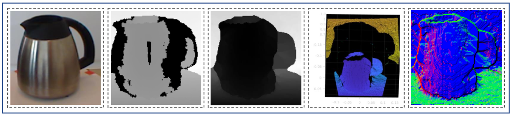
For depth domain, we first need appropriate RGB-like representation of depth data to leverage the power of pretrained CNN models over the large-scale RGB dataset of the ImageNet. To do so, there are several ways to represent depth data as RGB-like images such as HHA method of 7 (i.e. using horizontal and vertical observation values and angle of the normal to common surface), ColorJet work by 4 (i.e. mapping depth values to different RGB color values), or commonly used surface normal based colorization as in (1; 2). In this work, we prefer to use the colorization technique based on surface normals, as it confirms its effectiveness in our previous work (2). However, unlike surface normal estimation from depth maps without camera parameters in (2), we improve this in a more accurate way by estimating surface normals on 3D point clouds that have been computed using depth maps and camera intrinsic parameters. To address the issue of missing depth values, we first apply a fast vectorized depth interpolation by applying a median filter through a $5\times 5$ neighborhood to reconstruct missing values in noisy depth inputs. Then, 3D point cloud estimation by using camera intrinsic constants and surface normal calculation on point clouds are followed, respectively. After this, the common approach is scaling surface normals to map values to the $0-255$ range to fit RGB image processing. However, since such an approach of mapping from floating point to integer values leads to a loss of information, we use these normal vectors as is without performing further quantization or scaling. Furthermore, unlike in RGB input processing, we apply resizing operation on these RGB-like depth data using the nearest neighborhood based interpolation rather than bilinear interpolation. Because the latter may lead to more distortion in geometric structure of a scene. Moreover, nearest neighbor interpolation is more suitable to the characteristics of depth data by providing a better separability between foreground and background in a scene. When applying z-score standardization to depth domain, we use the standard-deviation of the ImageNet as in RGB domain. However, we use zero-mean instead of the ImageNet mean as normal vectors are in the range of $[-1,1]$ without the need for zero-mean shifting.

In this work, we employ several available pretrained models of PyTorch including AlexNet (10), VGGNet (14) (specifically VGGNet-16 model with batch normalization), ResNet (8) (specifically ResNet-50 and ResNet-101 models), and DenseNet (9). We extract features from seven different levels of CNN models. The models investigated in this study with the feature extraction levels are shown in Fig. 2. Each level of the CNN models shows name of the level, operations performed in the level with the number of them if exist (for ResNet (8) and DenseNet (9) models), and dimensions of the activation output.

We evaluate different baseline CNN models within our framework in terms of computational time and memory requirements. We evaluate the proposed framework in two parts: (i) Feature extraction containing CNN-RNN stages and (ii) Classification where a model based on the extracted features is learnt to distinguish the different classes. The batch size is set to 64 for all the models. Table 1 reports computational times and memory workspaces for the whole data processing ($41,877$ images) on Washington RGB-D dataset. The results here are the average results of two splits on RGB images. There is additional cost for depth data processing as it is required to colorize them. The results on this table cover the overall processing and classification of all $7$ level features. Moreover, it should be noted that classification time covers both training and testing processes, in which training takes the main computational burden. Therefore, the main cost in terms of processing time comes from training SVM models that works on CPU for $7$ times. The process for only a single optimum level would reduce the computational time to a ratio of seven approximately. Hence, using a single optimum level or fusion of selected levels can be efficient enough in terms of time and memory requirements while presenting sufficient representations.

An RNN in this study is of one-level structure with a single parent computation, which is obviously computationally fast comparing to the multi-level structural RNNs. Furthermore, in this way, it provides an ease of use with no need of further processing for fixing the required input forms. However, in order to testify the performance of single-level RNNs over multiple-level RNNs, we analyze the comparative accuracy performances of 1-level RNNs together with 3-levels RNNs (see Fig. 2 in main paper). To this end, we conduct experiments on two CNN activation levels with highest semantic information (L6 and L7) of the baseline model of AlexNet. The average results of two splits for both of RGB and depth data are shown in Fig. 3. The results show that RNN with 1-level performs better than RNN with 3-levels on RGB data, while 3-levels of RNN is better than 1-level of RNN on depth data. The better performance of RNN with 3-levels on depth data might be due to the use of a pretrained CNN model based on the RGB data of ImageNet. Hence, further processing might provide more representative information for depth data in that way. Therefore, this difference might be diminished or turn in favor of 1-level RNNs in the use of finetuned CNNs for depth modality as well. Overall, considering both RGB and depth data together, RNNs with 1-level are better in terms of accuracy performance as well.

We have shown that a fixed pretrained CNN model together with random RNN already achieves impressive results on a single level. Likewise, when such pretrained models are finetuned on depth data, the results are boosted greatly. The best single levels for RGB and depth data, respectively, are L4 and L5 for AlexNet; L5 and L6 for ResNet-101; and L6 and L7 for DenseNet-121. Next, to further improve accuracy performances, we investigate empirical accuracy analysis of multi-level fusions using fixed pretrained CNN models on RGB data and finetuned CNN models on depth data. In this work, in addition to the feature concatenation as in our previous work (2), we also apply average voting based on SVM confidence scores on the best performing levels. Table 2 reports the average accuracy on the all 10 train/test splits of Washington RGB-D dataset for AlexNet, DenseNet-121, and ResNet-101. The table shows the top four level results (best levels) for each modality and their fusion combinations. The best four levels (LB1, LB2, LB3, LB4) of AlexNet are (L4, L5, L6, L3) on RGB data and (L5, L6, L7, L4) on depth data, respectively; of ResNet-101 are (L5, L6, L4, L7) on RGB data and (L6, L7, L5, L4) on depth data, respectively; and for DenseNet-121 these levels are (L6, L5, L7, L4) on RGB and (L7, L6, L5, L4) on depth data, respectively. As can be seen from the table, a single level has already produced very good results. Since both model structures and data modality characteristics are different, the best results for each column generally vary depending on the data type and the used model. Nevertheless, in general, average voting on SVM confidence scores gives better results comparing to feature concatenation. We can also see that fusion of more levels does not necessarily increase the accuracy success. In general, the optimum results are achieved with SVM average voting of the best three levels for ResNet-101 and DenseNet-121 models.

In our previous work (2), we analyze the comparison of CNN-only features with the CNN-RNN incorporation-based features on best performing middle layers and show the advantages of using CNN-RNN. On the other hand, as we stated in the main paper, features obtained from semantically rich information-based final layers is often utilized in many approaches (13; 11; 6; 12; 5). Therefore, here we also extract features from the final semantic layer, level 7, and classify them with a linear SVM and report the results in Table 3. We use the finetuned models of AlexNet, DenseNet-121, and ResNet-101 models. RGB-D results are computed using the average RGB and depth SVM confidence scores. The results confirm that the backbone models produce impressive performance by finetuning the CNN models properly (see finetuning parameter setups in the main paper for more details). In addition, we can see that in case of CNN features powered by the incorporation of RNNs with the stronger representations (see object recognition performance in the main paper), the results are better compared to the CNN-only semantic features. Moreover, there is no any extra training cost, since RNNs in our model do not require training.

References

- Depth kernel descriptors for object recognition. In 2011 IEEE/RSJ International Conference on Intelligent Robots and Systems, pp. 821–826. Cited by: §1.
- Exploiting multi-layer features using a cnn-rnn approach for rgb-d object recognition. In The European Conference on Computer Vision (ECCV) Workshops, Cited by: §1, §5, §6.
- Imagenet: a large-scale hierarchical image database. In Computer Vision and Pattern Recognition, 2009. CVPR 2009. IEEE Conference on, pp. 248–255. Cited by: §1.
- Multimodal deep learning for robust rgb-d object recognition. In Intelligent Robots and Systems (IROS), 2015 IEEE/RSJ International Conference on, pp. 681–687. Cited by: §1.
- Learning hierarchical features for scene labeling. IEEE transactions on pattern analysis and machine intelligence 35 (8), pp. 1915–1929. Cited by: §6.
- Rich feature hierarchies for accurate object detection and semantic segmentation. In Proceedings of the IEEE conference on computer vision and pattern recognition, pp. 580–587. Cited by: §6.
- Learning rich features from rgb-d images for object detection and segmentation. In European Conference on Computer Vision, pp. 345–360. Cited by: §1.
- Deep residual learning for image recognition. In The IEEE Conference on Computer Vision and Pattern Recognition (CVPR), Cited by: Fig. 2, §2.
- Densely connected convolutional networks. In Proceedings of the IEEE Conference on Computer Vision and Pattern Recognition (CVPR), Cited by: Fig. 2, §2.
- Imagenet classification with deep convolutional neural networks. In Advances in neural information processing systems, pp. 1097–1105. Cited by: §2.
- RGB-d object recognition and pose estimation based on pre-trained convolutional neural network features. In Robotics and Automation (ICRA), 2015 IEEE International Conference on, pp. 1329–1335. Cited by: §6.
- Overfeat: integrated recognition, localization and detection using convolutional networks. In International Conference on Learning Representations (ICLR), Cited by: §6.
- CNN features off-the-shelf: an astounding baseline for recognition. In Proceedings of the IEEE conference on computer vision and pattern recognition workshops, pp. 806–813. Cited by: §6.
- Very deep convolutional networks for large-scale image recognition. In International Conference on Learning Representations (ICLR), Cited by: §2.