Climate Adaptation: Reliably Predicting from Imbalanced Satellite Data
Abstract
The utility of aerial imagery (Satellite, Drones) has become an invaluable information source for cross-disciplinary applications, especially for crisis management. Most of the mapping and tracking efforts are manual which is resource-intensive and often lead to delivery delays. Deep Learning methods have boosted the capacity of relief efforts via recognition, detection, and are now being used for non-trivial applications. However the data commonly available is highly imbalanced (similar to other real-life applications) which severely hampers the neural network’s capabilities, this reduces robustness and trust. We give an overview on different kinds of techniques being used for handling such extreme settings and present solutions aimed at maximizing performance on minority classes using a diverse set of methods (ranging from architectural tuning to augmentation) which as a combination generalizes for all minority classes. We hope to amplify cross-disciplinary efforts by enhancing model reliability.
1 Introduction
The last decade has witnessed tremendous growth both in computational power and scientific methods for pattern recognition and data science. Machine Learning is a tool driving many technologies across diverse sectors. However the fuel that drives this growth is data, and as is with every fuel it’s not directly usable. A critical problem is class imbalance, both in supervised and unsupervised form of learning algorithms. A dataset can be treated as imbalanced if there is a noticeable mismatch between the target variable and other values. For example, medical-diagnostics data is conventionally biased towards the negative class (healthy samples are more numerous than the infected ones). Other examples include fraud detection, natural language processing, visual recognition, astronomy, etc. Experimentally, high instability in performance has been observed in vanilla models when tested on imbalanced datasets Buda2018ASS.
Commonly, deep-net models are built to maximize predictive accuracy (ex. classification) but this metric is uneventful for the cases with limited labels, extreme classification etc. Lipton19. This happens because the trained classifier focuses only on the most-numerous class (since it has a higher proportion) while remaining below-par on minority classes. This may prove catastrophic in critical use cases like medical diagnostics and self-driving cars where the rare instances are of utmost importance.
Our use case consists of satellite imagery of African region which is labelled to help automate the process of predicting drought, cattle sustenance etc. via estimating the quality of forage droughtdataWandB. Usually, non-profit organizations cannot employ a dedicated team of ML engineers/researchers or clusters of GPUs Ferreira2019AnAN, models that can perform robustly and reliably at low requirements can be pragmatically utilized by domain-experts and local administration Pradhan2019SmarterPF for easy deployment.
Presently, researchers tend to tackle the imbalance issues (either at input or intermediate pipeline) in its narrow context with domain-specific solutions. We present drawn-out insights on several techniques to mitigate data-imbalance problems. The contributions of this paper are:
- •
We use a deep generative model for synthetic data augmentation of multi-spectral images. To the best of our knowledge, this specific area is still unexplored.
We also show that certain spectral bands are better for particular tasks (here, vegetation area analysis). - •
We show that a combination of Cyclic Learning Rate (CLR) CyclicalLR + Stochastic Weight Averaging (SWA) Izmailov2018AveragingWL is suitable for extreme imbalance scenarios.
- •
We further cement the compatibility of LDAM: Label-distribution aware loss-function LDAM, which works better than crude re-sampling and can be further improved by using class-balanced loss Cui2019ClassBalancedLB.
The rest of this paper is as follows: Section 2 introduces the dataset. Section 3 provides details on our modifications to the base neural-net model. It also includes subsections on Loss Function (3.1) which gives an overview of sampling functions, Cyclic Learning Rate (3.2) which is a popular training routine, and Stochastic Weight Averaging (3.3) as a powerful regularizer for handling data-imbalance issues. Section 4 provides details on multi-spectral imagery from the lens of machine learning. Section 5 presents our experiments with synthetic data augmentation followed by our overall results. Finally we conclude the paper in Section 7 with a short discussion on performance metrics.
We use intra-class variance (ICV), Balanced accuracy Brodersen2010TheBA and Recall as performance metrics (definitions in Sec. 1.1).
We present all our observations in two graph plots -
Figure 2 (ValAcc vs ICV) and Figure 3 (BalAcc vs ICV).
Our codebase- https://github.com/JARVVVIS/drought.
1.1 Performance Metrics
As we see in Lipton19; Sokolova2009ASA; RoccaTDS; BoyleTDS, accuracy is not the best metric to evaluate imbalanced datasets, as it can be very misleading. Metrics that provide better insights Sajjadi2018 include:
- •
Recall: Recall portrays the fraction of true positives could be detected correctly, It is defined as , Thus a low recall signifies a high number of false negatives which is undesirable in a real-world setting.
- •
Balanced Accuracy (BalAcc): The arithmetic mean of the TPR (True Positive Rate) and TNR (True Negative Rate). Thus if the model is exploiting the class-imbalance problem itself to increase the vanilla accuracy, the balanced accuracy will drop significantly and reflect the poor performance.
- •
Intra-Class Variance (ICV) :
(where denotes the validation accuracy and denotes the accuracy of the class for a given experiment). The aim is expose the models which have high category-variance (per-class accuracies) owing to overfitting on the frequent class (in comparison to robust models i.e. low variance). Em2017IncorporatingIV highlights importance of ICV for visual recognition tasks.
Table 8presents a comparative list of our final results as per the aforementioned benchmarks.
2 Data-set
The expert-labelled, multi-spectral satellite (LANDSAT) data droughtdataWandB was released as a bid to enhance drought detection pipelines. It essentially consists of 100,000 images split into 86,317 training and 10,778 validation images, having a spatial resolution of 65x65 pixels over 10 spectrum bands. Each image is labeled by a human expert as- ’the number of cows the geographical location at the center of the image can support’, serving as a measure of forage quality of the location and further as an indicator of whether the location is arid (drought-hit).
The dataset is highly imbalanced (roughly 60% of the data gathered is of class 0, classes 1 and 2 have 15% each, and the remaining 10% is class 3). The model can erroneously achieve 60% accuracy just by predicting 0 every time. However, such high mis-classification is very problematic since these algorithms will be deployed in high-stake real-world settings. We would like to make dense predictions no matter the location of the pixel, since there is high amount of sparsity in the labels. Hence, we need to train a model that is satisfactorily robust to out-of-distribution (o.o.d) samples and generalizes well on all the inherent classes i.e. independent-&-identically-distributed (i.i.d) samples. We focus on striking a pragmatic balance.
3 Network Architectures
Ever since winning the 2015 ILSVRC imagenet challenge ResNet resnet has inspired a family of deep convolutional neural networks. The skip connections in ResNet allow one to build deep networks (up to 1000 layers) while still keeping them optimizable, He et. al resnet demonstrated that even for fixed baseline architecture increase in depth almost always leads to increased accuracy.
While Scaling in depth resnet is the go-to method to boost a network’s accuracy, other less popular scaling methods include scaling by width Zagoruyko2016WideRN and resolution GPipe. Tan et. al Tan2019EfficientNetRM in their work showed that while scaling (in width, depth, resolution) improves model accuracy, the accuracy saturates after a certain level. They argued that different scaling dimensions (height, width, resolution) are not independent and the key to successfully scale deep networks is in balancing scaling in different dimensions rather than scaling in one direction only. To harmonize the scaling in all dimensions they proposed a compound scaling method which utilized (compound scaling coefficient) to uniformly scales the network’s depth, width and resolution. Depth : d = , Width : w = , Resolution : r = s.t.
However, scaling doesn’t change the core layer operations making it imperative to have a solid baseline network for achieving desired outcomes, Tan et al. Tan2019EfficientNetRM leveraged Neural Architecture Search NASZoph2016NeuralAS to propose a new baseline ”Efficient-Net” by optimizing for both accuracy and FLOPS.
Model Training Details Validation Acc Recall 0 1 2 3 ResNet-50 Learning Rate : 1e-3 Loss : Cross-Entropy 0.7465 0.9102 0.4198 0.5511 0.5682 Efficient-Net B4 Learning Rate : 1e-3 Loss : Cross-Entropy 0.7630 0.9199 0.4114 0.5739 0.6469
In Table 1 we give a baseline for ResNet-50 and Efficient-Net B4. We also apply standard data augmentation e.g. Random Horizontal-Flips, Random Vertical-Flips and Random Rotation after normalizing the data.
3.1 Loss Function and Sampling
Model Training Details Validation Acc Recall 0 1 2 3 ResNet-50 Learning Rate : 1e-3 Sampler : Loss : Cross-Entropy 0.7184 0.8154 0.5818 0.5014 0.6880 ResNet-50 Learning Rate : CLR Sampler : Loss : LDAM+DRW 0.7022 0.7792 0.5719 0.5780 0.6334 - Efficient-Net B4 Learning Rate : 1e-3 Loss : Cross-Entropy 0.7630 0.9199 0.4114 0.5739 0.6469 Efficient-Net B4 Learning Rate : CLR Sampler : Loss : LDAM+DRW 0.7196 0.7867 0.5900 0.5648 0.7699
Deep learning networks for all their might still fare very poorly on highly imbalanced datasets. Re-sampling and Re-weighting are the most common techniques used to cope with class imbalance problem.
- 1.
Re-sampling :
- (a)
Oversampling relay2016; Zhong2016; Buda2018ASS; Byrd2019WhatIT : Augmenting the dataset with multiple copies of minority class samples, however since we inherently have low information about the minority class oversampling more often than not leads to overfitting on minority class Cui2019ClassBalancedLB.
- (b)
Undersampling He2009LearningFI; Japkowicz2002TheCI; Buda2018ASS: Undersampling is achieved by rejecting samples from the more-frequent classes. Since we are loosing out on purpose in order to equalize the class-count, undersampling technique aren’t possible in case of high class imbalance Cui2019ClassBalancedLB.
- (a)
- 2.
Re-weighting Huang2016LearningDR; Huang2019DeepIL: Different set of weights (,where = total samples of class) are assigned to different classes. However re-weighting techniques cause instability in network’s optimization under extreme class imbalance Cui2019ClassBalancedLB; relay2016; Byrd2019WhatIT.
Both re-sampling and re-weighting conclusively aim to augment the training distribution to become much more identical to the test distribution. However, due to the aforementioned flaws performance of minority class is generally increased on the cost of the network’s ability to learn the majority class well.
Cao et al. LDAM designed a label-distribution aware loss function (LDAM) that regularizes the minority class much more strongly than the majority class, motivating the network to improve generalization on the minority class without suppressing the network’s ability to learn the majority class. Strong regularisation here can be understood in terms of enforcing bigger margins for the minority class as compared to the majority class. Moreover this approach is orthogonal to re-weighting and re-sampling, ensuring flexibility depending on level of imbalance in one’s dataset.
In the same work, Cao et al. LDAM proposed a “deferred re-balancing training” procedure which divides the training procedure into two stages. The first stage uses Empirical Risk Minimization with LDAM loss, learning a good initial representation. The second stage employs re-weighted LDAM loss with a smaller learning rate. The main rationale behind this is to bypass the problems caused by re-weighting in the optimization process of a Neural Network by first learning a good initial representation and then optimizing on that. We also employ a re-sampling scheme () orthogonal to the LDAM+DRW routine. Table 2 presents our results with LDAM.
In the next subsection on CLR, we briefly discuss the advantages of Cyclic Learning Rate and later establish it’s compatibility and usefulness for imbalance scenarios.
3.2 Cyclical Learning Rates (CLR)
| Training Details | Values |
| Upper Bound | 1e-3 |
| Lower Bound | 1e-5 |
| Stepsize | 2 |
| Functional Form | Triangular |
Learning rate is responsible for scaling the gradients at each weight update and is one of the most important hyper-parameters to tune while training a deep neural network as too small a learning rate will encourage very small steps and hence the network might not converge at all, whereas too high a learning rate will propel divergent behavior. The optimal learning rate depends on the network’s loss surface and usually is not feasible to calculate.
The cyclical learning rate CyclicalLR oscillates between a range of values, going against the conventional wisdom of exponentially/step-wise decreasing the learning rate as training progresses. The advantages of doing this are -
- 1.
Stuck on a sharp minimum Li2018VisualizingTL - Networks with flatter minima tend to be more robust than the ones with sharp minima, as flatter minima ensure that we are in optimal minima region in the test loss surface as well and hence generalize better, periodically increasing the value of learning rate will help to get out of the sharp minima more quickly.
- 2.
Stuck on saddle points Jin2017HowTE; CyclicalLR - When training a Deep network it is very likely that the loss surface topology contains a lot of saddle points. Thus having per periodic boost of high learning rate is very useful as it helps in traversing the saddle points more quickly (since the gradient value is already very low here).
Experimental values are given in Table 3.
In combination with CLR, we use Stochastic Weight Averaging (SWA) which is a very promising regularization technique. We outline it’s benefits for our problem and the setup details in the following subsection.
3.3 Stochastic Weight Averaging (SWA)
Model Training Details Validation Accuracy Recall 0 1 2 3 Efficient-Net B4 Learning Rate : 1e-3 Loss : Cross-Entropy 0.7630 0.9199 0.4114 0.5739 0.6469 Efficient-Net B4 Stochastic Weight Averaging : No Learning Rate : CLR Sampler : Loss : LDAM+DRW 0.7196 0.7867 0.5900 0.5648 0.7699 Efficient-Net B4 Stochastic Weight Averaging : Yes Learning Rate : CLR Sampler : Loss : LDAM+DRW 0.7292 0.8098 0.6017 0.5409 0.7436
Another go-to methodology machine learning practitioners generally adopt while training models is ensemble learning. Ensemble learning improves predictions by combining [for example voting, averaging etc] results of various models. However when training Deep Neural Networks it is not possible to train multiple models on the dataset due to time and compute constraints.
Garipov et al. Garipov2018LossSM in their work on Fast Geometric Ensembles showed that using cyclical learning rates with stochastic gradient descent traversed on the periphery of the optimal weights but never quite reached it’s center, They selected the network with weights on the periphery to form the ensemble. This helped in training the ensemble in the time required to train one network.
Stochastic Weight Averaging Izmailov2018AveragingWL uses the same setup i.e. high frequency cyclical/constant learning rate with SGD to traverse around the optimal weight set, and then does averaging in the weight domain only at different snapshots of training. This allows weights to reach the much desired optimal set. The advantages of this are following:
- 1.
Faster inference time compared to Garipov et al. Garipov2018LossSM, as we only have one model as the end result, compared to waiting for k results from k models.
- 2.
Given that the underlying data distribution is the same, it is fair to assume that the test and train datasets will have similar loss surfaces. Thus it makes much more sense to aim for a more flatter minima while training than a sharp one [even if it leads to higher training error], as it will ensure that we are in an optimal minima region in the test loss surface as well, leading to a more robust network.
We find that using SWA in combination with Adam optimizer and the CLR setup we were able to significantly improve the low/mid class accuracy and subsequently train a more robust network Table 4.
In the next section we present our brief insights connecting remote sensing knowledge with research in machine learning. The bands are a key component and must be studied in more detail for better cross-linking when being used with neural networks.
4 Training On Subset of Bands
Model Training Details Validation Accuracy Recall 0 1 2 3 Efficient-Net B4 Bands: All Stochastic Weight Averaging : Yes Learning Rate : CLR Sampler : Loss : LDAM+DRW 0.7292 0.8098 0.6017 0.5409 0.7436 Efficient-Net B4 Bands: 4,3,2 Stochastic Weight Averaging : Yes Learning Rate : CLR Sampler : Loss : LDAM+DRW 0.7047 0.7996 0.5356 0.5475 0.6428 Efficient-Net B4 Bands: 5,4,3 Stochastic Weight Averaging : Yes Learning Rate : CLR Sampler : Loss : LDAM+DRW 0.7022 0.7792 0.5719 0.5780 0.6334 Efficient-Net B4 Bands: 6,5,2 Stochastic Weight Averaging : Yes Learning Rate : CLR Sampler : Loss : LDAM+DRW 0.7441 0.8156 0.5941 0.6138 0.7584
Multi-spectral Images (MSI) are described by 3 to 10 narrow spectral bands. This high spectral information is very beneficial as by combining different spectral bands we can infer different information, leading up to terabytes of data produced per day.
Since adjacent bands in MSI are highly correlated, there is a lot of redundancy in our data. This contrary to conventional wisdom, leads to degradation of accuracy on increasing the number of bands in MS images BS, also using too many spectral bands incur high computational cost as well as more inference time.
Thus it makes sense to use only those spectral bands which motivate the network to learn better feature representations for separating specific classes. The selected band performance is often conditional on many aspects of the classification pipeline such as the nature of the adopted classifier and its parameter configurations HBS.
A major hurdle was deciding the importance of each spectral band, since there is not a lot of literature specific to neural networks. We experimented with three different band combinations based on their characteristics. Focareta2015
- 1.
4-3-2: Natural Color This band combination results in the image appearing as perceived by the human eye.
- 2.
5-4-3: Near Infrared Composite This combination contains near-infrared(5), red(4), green(3) bands, This combination is particularly useful while analyzing vegetation, crops and wetlands as it is able to capture the near-infrared light reflected by chlorophyll.
- 3.
6-5-2: Agriculture It is a combination of SWIR-1 (6), near-infrared (5) and blue (2). The short-wave and near infrared allows this combination to be used for crop monitoring.
As observed in Table 5, the combination 6-5-2 seems to work the best for the given dataset.
We believe the original dataset is small but inherently complex due to overlap of several spectral bands and thus data augmentation is very beneficial. The next section expands on the data generation component of our project.
5 Generating Synthetic Images
Model Training Details Validation Accuracy Recall 0 1 2 3 Efficient-Net B4 Learning Rate : 1e-3 Loss : Cross-Entropy Dataset : Original 0.76 0.9199 0.4114 0.5739 0.6469 Efficient-Net B4 Stochastic Weight Averaging : No Learning Rate : 1e-3 Sampler : Loss : Cross-Entropy Dataset : GAN-Augmented 0.67 0.6815 0.6619 0.6258 0.7521 Efficient-Net B4 Bands: 6,5,2 Stochastic Weight Averaging : Yes Learning Rate : CLR Sampler : Loss : LDAM+DRW Dataset : Original 0.74 0.8156 0.5941 0.6138 0.7584 Efficient-Net B4 Stochastic Weight Averaging : Yes Learning Rate : CLR Sampler : Loss : LDAM+DRW Dataset : GAN-Augmented 0.70 0.7459 0.5842 0.5540 0.7436
| Training Details | Values |
| Resolution | 64x64 |
| Epochs | 45 |
| Learning Rate | 2e-4 |
| 0.5 | |
| 0.999 |
The introduction of Generative Adversarial Networks (GANs) Goodfellow2014GenerativeAN sprung up many exciting research directions, the field has grown steadily with numerous applications in image super-resolution, in-painting, image-to-image translation, image enhancement (For example, earth observation/remote sensing Liu2018PSGANag; Tsagkatakis2019SurveyOD).
Standard data augmentation has been used as a go-to technique for enhancing generalizability. Generative adversarial networks offer a novel method for data augmentation Sandfort2019DataAU, but have still not been adopted by either the earth observation or remote sensing community. We use DC-GAN Radford2015UnsupervisedRL, which employs deep convolutional neural networks for both the Generator (G) and Discriminator (D), to generate synthetic images for the low represented classes as a form of data-augmentation to equalize the number of samples of each class. We only operate on a subset of bands (6-5-2), since it is easier to critic the visual perceptibly of images this way than all the bands combined.
The main motivation behind equalizing the number of classes was to make the network learn improved discriminatory features and hence becomes more robust.
We monitored the visual perceptibly of generated images over the training period (60 epochs) and found that the network converges at about 45 epochs, see Figure 4. The final dataset (GAN-Augmented) consisted of 120,000 images with 30,000 images from each class. The architectures used for D and G are kept same as described in Radford2015UnsupervisedRL. Training details are shown in Table 7 and Loss plots are in Figure 1.
Table 6demonstrates the results we obtained from the network (in combination with various training methodologies) on the GAN-Augmented dataset, a significant increase in the per-class accuracies of rare-classes was observed.


6 Results
Model Training Details Validation Acc Balanced Validation Acc Intra-Class Variance ResNet-50 Learning Rate : 1e-3 Loss : Cross-Entropy 0.7465 0.6123 0.4510 ResNet-50 Learning Rate : 1e-3 Sampler : Loss : Cross-Entropy 0.7184 0.6467 0.2757 ResNet-50 Learning Rate : CLR Sampler : Loss : LDAM+DRW 0.7022 0.2076 0.6406 Efficient-Net B4 Learning Rate : 1e-3 Loss : Cross-Entropy 0.7630 0.6380 0.4443 Efficient-Net B4 Learning Rate : CLR Sampler : Loss : LDAM+DRW 0.7196 0.6779 0.2185 Efficient-Net B4 Stochastic Weight Averaging : Yes Learning Rate : CLR Sampler : Loss : LDAM+DRW 0.7292 0.6740 0.2417 Efficient-Net B4 Bands: 6,5,2 Stochastic Weight Averaging : Yes Learning Rate : CLR Sampler : Loss : LDAM+DRW 0.7441 0.6955 0.2115 Efficient-Net B4 Stochastic Weight Averaging : No Learning Rate : 1e-3 Sampler : Loss : Cross-Entropy Dataset : GAN-Augmented 0.67 0.6803 0.0942 Efficient-Net B4 Stochastic Weight Averaging : Yes Learning Rate : CLR Sampler : Loss : LDAM+DRW Dataset : GAN-Augmented 0.70 0.6569 0.1967
We evaluate various techniques in a combination setting to facilitate training of robust Deep Neural Networks. We provide baseline metrics for both architectures (ResNet-50 and Efficient-Net B4) in Table 1, and observe that the baselines fall prey to overfitting owing to high class imbalance. Table 2 advocates LDAM loss as a label-dependent regularizer which leads to a reduction in Intra class variance (ICV) and improvements in balanced-accuracy, see Figure 3. We observe that performance of SWA+LDAM+CLR (all bands, Table 8 - 6) performs compared to SWA+LDAM+CLR6,5,2 (Table 8 - 7).
Lastly we present the results of baseline as well as SWA+LDAM+CLR6,5,2 on GAN-Augmented dataset. There is a substantial decrease in ICV while maintaining decent balanced-accuracy in the baseline experiment, indicating that the network was able to learn better discriminative features for all rare-classes. The SWA+LDAM+CLR6,5,2 though under-performing on aspect of per-class accuracy leads to considerable decrease in ICV, see Figure 3.
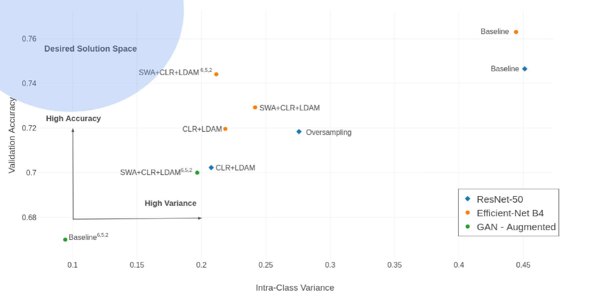
The solutions at the top-left section (more accurate, less variant respectively) of the graph are most desirable (i.e. robust).
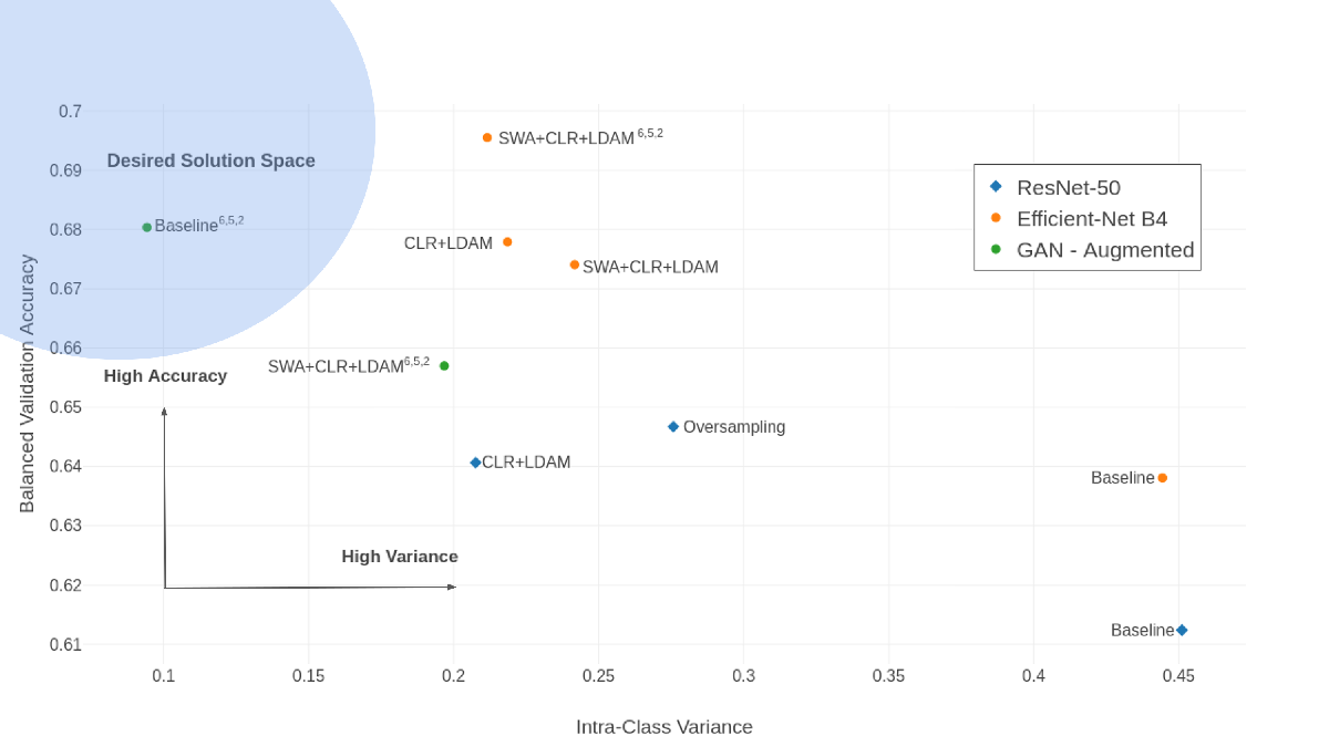
We observe various models which were performing very well as per the vanilla validation-accuracy plummet when plotted w.r.t. balanced validation accuracy thus exposing the deep-rooted focus on the frequent class and futility of ValAcc.
6.1 Limitations
- •
In Figure 3 (BalAcc vs ICV) we observe one outlier result: SWA+CLR+LDAM 6,5,2 -GAN Augmented, as per our trend this should have been the best result (instead it is the Baseline - GAN Augmented). This exception may be attributed to incomplete insights on the GAN data interaction with our network modifications.
- •
Problems with generating data for all spectral bands. There is a lack of empirical data to ascertain quality of output data in such scenario. Liu2018PSGANag, Tsagkatakis2019SurveyOD, Kerdegari2019SemisupervisedGF. We expect improvements with higher-diversity images Ghosh2018MultiagentDG.
- •
We did not explore alternative generative models ex. Kernel-based GANs Mehrjou2019KernelGuidedTO, Variational Autoencoders family (VQ-VAEs Oord2017NeuralDR-VQVAE; Razavi2019VQVAE2, hybrid VAE-GAN Larsen2015VAEGAN).
- •
No class-activation mapping for model explanation or other interpretability mechanism Zhou2016LearningDF; Selvaraju2016GradCAMVE; Hooker2019ABF.
- •
We did not incorporate adversarial training/defense.


7 Conclusion
There is a lot of focus on handling or curbing the adverse effects of imbalanced data. Mitigating class imbalance is an important research area, as it will allow trust-worthy solutions in the form of deep neural networks in many eclectic fields. As per trend, deep learning networks are tuned to maximize the total accuracy over the entire dataset, thus focusing on the majority-class samples. As a result, the models under-perform on minority class(es) samples leading to bad intra-class generalization and low robustness.
We provide a comparative overview of diverse yet latest methodologies for operating on skewed datasets that is suffering from class-imbalance problems. This diverse set of techniques ranges from discussions on state-of-the-art convolutional neural network architectures, label-dependent loss functions, learning-rate routines, generating Deep Neural Network ensembles and finally generating data samples using DC-GAN.
We conclusively aspire to serve as a toolkit for practitioners and researchers suffering from skewed data problems in their respective fields as we present the work to other domain-experts, especially those dealing with multiple minority classes. Since our ensemble methodology doesn’t overfit on the rare classes but tries to generalize on the non-major classes thus achieving a trade-off on overall accuracy but high robustness.
Acknowledgements
We would like to thank Meenakshi Sarkar and Shivam Saboo for insightful discussions, also the anonymous reviewers for their valuable feedback on the draft. Authors would like to give a shout-out to Weights & Biases and to the ICLR’20 CCAI Workshop’s Mentorship Program.
PP extends special thanks to Debasish Ghose (IISc-B) and Krikamol Muandet (MPI-IS) for supporting this work.
References
- (1) Tara Boyle. Dealing with imbalanced data, 2019. towardsdatascience.com.
- (2) Kay Henning Brodersen, Cheng Soon Ong, Klaas Enno Stephan, and Joachim M. Buhmann. The balanced accuracy and its posterior distribution. 20th International Conference on Pattern Recognition (ICPR), pages 3121–3124, 2010.
- (3) Mateusz Buda, Atsuto Maki, and Maciej A. Mazurowski. A systematic study of the class imbalance problem in convolutional neural networks. Neural networks, 106:249–259, 2018.
- (4) Jonathon Byrd and Zachary Chase Lipton. What is the effect of importance weighting in deep learning? In International Conference on Machine Learning (ICML), 2019.
- (5) Kaidi Cao, Colin Wei, Adrien Gaidon, Nikos Aréchiga, and Tengyu Ma. Learning imbalanced datasets with label-distribution-aware margin loss. In Advances in Neural Information Processing Systems (NeurIPS), 2019.
- (6) Yin Cui, Menglin Jia, Tsung-Yi Lin, Yang Song, and Serge J. Belongie. Class-balanced loss based on effective number of samples. In IEEE/CVF Conference on Computer Vision and Pattern Recognition (CVPR), pages 9260–9269, 2019.
- (7) Yan Em, Feng Gao, Yihang Lou, Shiqi Wang, Tiejun Huang, and Ling yu Duan. Incorporating intra-class variance to fine-grained visual recognition. IEEE International Conference on Multimedia and Expo (ICME), pages 1452–1457, 2017.
- (8) João Ferreira, Gustavo Rau de Almeida Callou, Albert Josua, Dietmar Tutsch, and Paulo Maciel. An artificial neural network approach to forecast the environmental impact of data centers. Information, 10:113, 2019.
- (9) Mariano Focareta, Salvo Marcuccio, Silvia Liberata Ullo, and C. Votto. Combination of landsat 8 and sentinel 1 data for the characterization of a site of interest. a case study: the royal palace of caserta. In Proceedings of the 1st International Conference on Metrology for Archaeology, 2015.
- (10) Timur Garipov, Pavel Izmailov, Dmitrii Podoprikhin, Dmitry P. Vetrov, and Andrew Gordon Wilson. Loss surfaces, mode connectivity, and fast ensembling of dnns. In Advances in Neural Information Processing Systems (NeurIPS), 2018.
- (11) Arnab Ghosh, Viveka Kulharia, Vinay P. Namboodiri, Philip H. S. Torr, and Puneet Kumar Dokania. Multi-agent diverse generative adversarial networks. 2018 IEEE/CVF Conference on Computer Vision and Pattern Recognition (CVPR), pages 8513–8521, 2018.
- (12) Ian J. Goodfellow, Jean Pouget-Abadie, Mehdi Mirza, Bing Xu, David Warde-Farley, Sherjil Ozair, Aaron C. Courville, and Yoshua Bengio. Generative adversarial nets. In Advances in Neural Information Processing Systems (NIPS), 2014.
- (13) P. Groves and P. Bajcsy. Methodology for hyperspectral band and classification model selection. In IEEE Workshop on Advances in Techniques for Analysis of Remotely Sensed Data, 2003, pages 120–128, 2003.
- (14) Haibo He and Edwardo A. Garcia. Learning from imbalanced data. IEEE Transactions on Knowledge and Data Engineering, 21:1263–1284, 2009.
- (15) Kaiming He, Xiangyu Zhang, Shaoqing Ren, and Jian Sun. Deep residual learning for image recognition. In Proc.. of IEEE Conference on Computer Vision and Pattern Recognition (CVPR), pages 770–778, Las Vegas, USA, June 2016.
- (16) Andrew Hobbs and Stacey Svetlichnaya. Satellite-based prediction of forage conditions for livestock in northern kenya, 2020. ICLR 2020 Workshop on Computer Vision for Agriculture (CV4A).
- (17) Sara Hooker, Dumitru Erhan, Pieter-Jan Kindermans, and Been Kim. A benchmark for interpretability methods in deep neural networks. In Advances in Neural Information Processing Systems (NeurIPS), 2019.
- (18) Chen Huang, Yining Li, Chen Change Loy, and Xiaoou Tang. Learning deep representation for imbalanced classification. IEEE Conference on Computer Vision and Pattern Recognition (CVPR), pages 5375–5384, 2016.
- (19) Chen Huang, Yining Li, Chen Change Loy, and Xiaoou Tang. Deep imbalanced learning for face recognition and attribute prediction. IEEE Transactions on Pattern Analysis and Machine Intelligence (TPAMI), 2019.
- (20) Yanping Huang, Yonglong Cheng, Dehao Chen, HyoukJoong Lee, Jiquan Ngiam, Quoc V. Le, and Zhifeng Chen. Gpipe: Efficient training of giant neural networks using pipeline parallelism. In Advances in Neural Information Processing Systems (NeurIPS), 2019.
- (21) Pavel Izmailov, Dmitrii Podoprikhin, Timur Garipov, Dmitry P. Vetrov, and Andrew Gordon Wilson. Averaging weights leads to wider optima and better generalization. In Conference on Uncertainty in Artificial Intelligence (UAI), 2018.
- (22) Nathalie Japkowicz and Shaju Stephen. The class imbalance problem: A systematic study. Intelligent data analysis, 6:429–449, 2002.
- (23) Chi Jin, Rong Ge, Praneeth Netrapalli, Sham M. Kakade, and Michael I. Jordan. How to escape saddle points efficiently. In International Conference on Machine Learning (ICML), 2017.
- (24) Hamideh Kerdegari, Manzoor Razaak, Vasileios Argyriou, and Paolo Remagnino. Semi-supervised gan for classification of multispectral imagery acquired by uavs. ArXiv, abs/1905.10920, 2019.
- (25) Anders Boesen Lindbo Larsen, Søren Kaae Sønderby, Hugo Larochelle, and Ole Winther. Autoencoding beyond pixels using a learned similarity metric. In International Conference on Machine Learning (ICML), 2015.
- (26) Hao Li, Zheng Xu, Gavin Taylor, and Tom Goldstein. Visualizing the loss landscape of neural nets. In Advances in Neural Information Processing Systems (NeurIPS), 2018.
- (27) Zachary C. Lipton and Jacob Steinhardt. Troubling trends in machine learning scholarship. Queue, 17(1):80:45–80:77, Feb. 2019.
- (28) Xiangyu Liu, Yunhong Wang, and Qingjie Liu. Psgan: A generative adversarial network for remote sensing image pan-sharpening. 2018 25th IEEE International Conference on Image Processing (ICIP), pages 873–877, 2018.
- (29) Arash Mehrjou, Wittawat Jitkrittum, Krikamol Muandet, and Bernhard Scholkopf. Kernel-guided training of implicit generative models with stability guarantees. ArXiv, abs/1910.14428, 2019.
- (30) Prabhu Pradhan, Meenakshi Sarkar, and Debasish Ghose. Smarter prototyping for neural learning. In Neural Information Processing Systems (NeurIPS) Workshop. OpenReview, 2019. ML-Retrospectives.
- (31) Alec Radford, Luke Metz, and Soumith Chintala. Unsupervised representation learning with deep convolutional generative adversarial networks. In International Conference on Learning Representations, (ICLR), 2016.
- (32) Ali Razavi, Aaron van den Oord, and Oriol Vinyals. Generating diverse high-fidelity images with vq-vae-2. In Advances in Neural Information Processing Systems (NeurIPS), 2019.
- (33) Baptiste Rocca and Joseph Rocca. Handling imbalanced datasets in machine learning, 2019. towardsdatascience.com.
- (34) Olga Russakovsky, Jia Deng, Hao Su, Jonathan Krause, Sanjeev Satheesh, Sean Ma, Zhiheng Huang, Andrej Karpathy, Aditya Khosla, Michael Bernstein, Alexander C. Berg, and Li Fei-Fei. ImageNet Large Scale Visual Recognition Challenge. International Journal of Computer Vision (IJCV), 115(3):211–252, 2015.
- (35) Mehdi S. M. Sajjadi, Olivier Bachem, Mario Lučić, Olivier Bousquet, and Sylvain Gelly. Assessing generative models via precision and recall. In Advances in Neural Information Processing Systems (NeurIPS), 2018.
- (36) Veit Sandfort, Ke Yan, Perry J. Pickhardt, and Ronald M. Summers. Data augmentation using generative adversarial networks (cyclegan) to improve generalizability in ct segmentation tasks. In Scientific Reports, 2019.
- (37) Ramprasaath R. Selvaraju, Michael Cogswell, Abhishek Das, Ramakrishna Vedantam, Devi Parikh, and Dhruv Batra. Grad-cam: Visual explanations from deep networks via gradient-based localization. 2017 IEEE International Conference on Computer Vision (ICCV), pages 618–626, 2016.
- (38) Li Shen, Zhouchen Lin, and Qingming Huang. Relay backpropagation for effective learning of deep convolutional neural networks. In Computer Vision – ECCV 2016, volume 9911 of Lecture Notes in Computer Science, pages 467–482, Cham, 2016. Springer International Publishing.
- (39) Leslie N. Smith. Cyclical learning rates for training neural networks. 2017 IEEE Winter Conference on Applications of Computer Vision (WACV), pages 464–472, 2015.
- (40) Marina Sokolova and Guy Lapalme. A systematic analysis of performance measures for classification tasks. Information Processing and Management, 45:427–437, 2009.
- (41) W. Sun and Q. Du. Hyperspectral band selection: A review. IEEE Geoscience and Remote Sensing Magazine, 7(2):118–139, 2019.
- (42) Mingxing Tan and Quoc V. Le. Efficientnet: Rethinking model scaling for convolutional neural networks. In International Conference on Machine Learning (ICML), 2019.
- (43) Grigorios Tsagkatakis, Anastasia Aidini, Konstantina Fotiadou, Michalis Giannopoulos, Anastasia Pentari, and Panagiotis Tsakalides. Survey of deep-learning approaches for remote sensing observation enhancement. In Sensors, volume 19, page 3929, 2019.
- (44) Aäron van den Oord, Oriol Vinyals, and Koray Kavukcuoglu. Neural discrete representation learning. In Advances in Neural Information Processing Systems (NIPS), 2017.
- (45) Sergey Zagoruyko and Nikos Komodakis. Wide residual networks. In British Machine Vision Conference (BMVC), volume abs/1605.07146. BMVA Press, 2016.
- (46) Qiaoyong Zhong, Chao Li, Yingying Zhang, Haiming Sun Shicai Yang, Di Xie, and Shiliang Pu. Towards good practices for recognition & detection. In CVPR Workshops, 2016.
- (47) Bolei Zhou, Aditya Khosla, Àgata Lapedriza, Aude Oliva, and Antonio Torralba. Learning deep features for discriminative localization. In IEEE Conference on Computer Vision and Pattern Recognition (CVPR), pages 2921–2929, 2016.
- (48) Barret Zoph and Quoc V. Le. Neural architecture search with reinforcement learning. In International Conference on Learning Representations, (ICLR), volume abs/1611.01578, 2017.