Blind Data Detection in Massive MIMO via -norm Maximization over the Stiefel Manifold
Abstract
Massive MIMO has been regarded as a key enabling technique for 5G and beyond networks. Nevertheless, its performance is limited by the large overhead needed to obtain the high-dimensional channel information. To reduce the huge training overhead associated with conventional pilot-aided designs, we propose a novel blind data detection method by leveraging the channel sparsity and data concentration properties. Specifically, we propose a novel -norm-based formulation to recover the data without channel estimation. We prove that the global optimal solution to the proposed formulation can be made arbitrarily close to the transmitted data up to a phase-permutation ambiguity. We then propose an efficient parameter-free algorithm to solve the -norm problem and resolve the phase-permutation ambiguity. We also derive the convergence rate in terms of key system parameters such as the number of transmitters and receivers, the channel noise power, and the channel sparsity level. Numerical experiments will show that the proposed scheme has superior performance with low computational complexity.
Index Terms:
Massive MIMO, blind data detection, non-convex optimization, Stiefel manifold.I Introduction
Massive multiple-input multiple-output (MIMO) can significantly enhance spectral efficiency and reduce interference in cellular networks, and thus has been regarded a key enabler for 5G and beyond networks[1]. However, the benefits heavily rely on accurate channel state information (CSI), which represents a major challenge, especially for systems with higher frequencies, e.g., millimeter wave (mmWave) massive MIMO systems [2]. It is largely due to the faster temporal variations and the large dimension of the channel matrix. A common approach is to send sufficient pilot symbols for reliable channel estimation, which then enables coherent data detection. However, with the limited coherence time and large dimension of the channel matrix, the pilot overhead will easily occupy too much radio resource. In addition, due to the limited number of orthogonal pilot sequences in multi-cell systems, pilot contamination will further jeopardize the performance of coherent massive MIMO systems [3]. To overcome this difficulty, blind data detection methods have been proposed to recover the data from the received signal without training pilots [4, 5, 6]. However, due to the degradation of the detection accuracy, traditional blind scheme can achieve a degrees of freedom (DoF) of for a massive MIMO system with transmit antennas and receive antennas in a rich scattering environment where is the coherence time [4], which is the same as that achieved by a coherent massive MIMO system taking account of the pilot overhead [7].
There have been some attempts to exploit the channel sparsity to reduce the pilot overhead. Many experimental studies have indicated the sparsity of massive MIMO channels in the angular domain due to the limited number of scatterers[8, 9]. By exploiting the sparsity of such channels, compressed-sensing-based channel estimation can reduce the pilot training[10], hence achieving a DoF of , where depends on the channel sparsity level [11]. However, the pilots for sparse channel estimation still lead to a DoF loss of the order of .
Recently, it has been shown that, with blind scheme, exploiting the sparsity structure of massive MIMO channels can further improve the performance [11, 12, 13, 14]. Particularly, Zhang et. al [11] showed that under some regularity conditions, blind detection can achieve a DoF arbitrarily close to for sparse massive MIMO channels. Approximate message passing (AMP)-based algorithms were proposed in [11] and [12] for blind data detection by exploiting the sparsity of the channel, which showed a superior performance. However, AMP-based approaches generally rely on certain assumptions on the probability density functions (PDF) of the channel and data, which is unrealistic in practical systems. Moreover, AMP-based approaches require an iterative message passing algorithm that leads to significant complexity due to the slow convergence rate for the large problem size in massive MIMO systems. In [13], a subspace-based method, which decomposes the covariance of the received signal into the subspace of the channel and refines the decomposition by exploiting the channel sparsity, was proposed in blind detection for massive MIMO. However, a long sample sequence of the received signal is required to estimate the covariance, which is applicable only with a very long channel coherence time and very low mobility. In addition, all of the aforementioned works fall short on the theoretical aspect, namely, they fail to provide a theoretical analysis for the achievable performance.
In this paper, we propose a novel formulation for blind data detection for sparse massive MIMO channels, supported by an efficient algorithm which does not require the knowledge of the PDF of the data and the channel. In addition, the proposed scheme does not contain tuning parameters, and can be implemented efficiently with a fast convergence rate. The theoretical justification of the formulation and the convergence rate of the algorithm are also developed. The main contributions are summarized as follows:
- •
Data Concentration Property:11 1 In this paper, the term concentration represents the concentration of measure phenomenon. This phenomenon can be informally expressed as “A random variable that depends in a Lipschitz way on many independent variables is essentially constant”[15]. In this paper, we exploit the statistical information of the data transmitted in general communication systems for a novel formulation of the blind detection problem. Specifically, we show that under mild conditions, there is a data concentration phenomenon, which enables a simple blind sparse recovery formulation of a massive MIMO system over the Stiefel manifold.
- •
Blind Detection via -norm Maximization: It was shown in [11] that the channel sparsity leads to a fundamental performance gain for the degrees of freedom of massive MIMO systems. Hence our proposed formulation leverages the sparsity structure of massive MIMO channels. Traditionally, -norm is the most widely used formulation to induce sparsity [16]. However, the non-smooth nature of the -norm results in low-convergence speed and high complexity [17]. In this paper, inspired by the smoothness and the fact that a high-order norm promotes sparsity [18, 19, 20, 21], we consider -norm maximization over the Stiefel manifold for blind data recovery of massive MIMO systems with sparse channels. Furthermore, we show that the global maximizer of the formulation is arbitrarily close to the true data up to a phase and permutation ambiguity for a sufficiently large number of antennas.
- •
Efficient Algorithm and Convergence Rate Analysis: By taking advantage of the smooth property of the -norm and the geometric structure of the Stiefel manifold, a parameter-free algorithm with low complexity is proposed for blind data recovery for massive MIMO systems. We show that under mild conditions, the proposed algorithm converges to the stationary point of the -norm maximization problem. We further show the convergence rate in terms of the key system parameters.
The rest of the paper is organized as follows. In Section II, we present the system model, the sparse MIMO channel and elaborate the data concentration property. In Section III, we present the -norm-based manifold optimization problem as a new formulation for blind data detection problem. We further discuss the structural properties of the optimal solution to the new formulation in the noiseless and noisy cases. A fast and parameter-free algorithms is proposed and the corresponding convergence analysis are given in Section IV. Numerical simulation results are provided in Section V. Finally, Section VI summarizes the work.
Notations: and denote the inverse and conjugate transpose of matrix , respectively. represents the null space of . is used to take an element-wise abstract value. represents a diagonal matrix constructed by using as the diagonal elements. The -th row vector and -th column vector in are and , respectively. represents the element in the -th row and -th column of . denotes the Hadamard product. denotes the ceiling operator. is the general inner product of and . Finally, , and are respectively, the Frobenius norm, spectral norm and induced norm of matrix .
II System Model
In this section, we introduce the system model of the considered massive MIMO system, followed by the sparse channel model and the data concentration property.
II-A System Model
Consider a single-cell mmWave massive MIMO communication system, as illustrated in Fig. 1. There are single-antenna users transmitting to a base station (BS) that is equipped with receive antennas with . Denote as the symbols transmitted by user within one frame. The aggregate transmit symbols of the users are denoted by . For simplicity, we consider a block flat fading channel, but the framework can be easily extended to OFDM systems. The received signal at the BS is given by
| (1) |
where is the transmit power of the users, is the aggregate MIMO channel matrix, is the channel matrix between the -th user and the BS, is the aggregate large-scale fading coefficients of the users to the BS, and is the aggregate additive channel noise of independent and identically distributed (i.i.d.) elements. We assume that the BS has knowledge of , which can be obtained in practice with a very low signaling overhead due to the slowly varying path gain.

II-B Sparsity of the mmWave MIMO Channel
The mmWave propagation environment is well characterized by a clustered channel model [22], which can be parameterized by paths of the -th user. The small-scale mmWave channel matrix between user and the BS during the coherence time is given by
| (2) |
where denotes the normalized path gain of the -th path for the -th user. We assume that are i.i.d. random variables following the complex Gaussian distribution , and denote the azimuth and zenith angles of arrival (AoA) of the -th path for the -th user, and represents the receive and transmit array response vectors. For simplicity, we assume that the BS is equipped with a uniform rectangular planar array (URPA) with and elements () in the horizontal and vertical direction, respectively. The array response vector is given by [23]
| (3) | ||||
where and .
The spatial aggregate channel of users can be expressed by a “virtual angular domain” representation as follows:
| (4) |
where is the steering matrix for the receive array. With an receive URPA, we have [24], where and are the unitary discrete Fourier transform (DFT) matrices. can be interpreted as the normalized channel gain between the -th user and the -th discrete receive angle [25]. From [8], the number of clusters is quite limited in the mmWave band. Furthermore, is usually quite large to mitigate the path loss effect in mmWave frequencies [26]. Hence, the number of paths is usually much smaller than the channel dimension, i.e., . Therefore, can be regarded as approximately sparse (or spiky).22 2 The reason why is not exactly sparse is the mismatch between the exact receive angle and the predefined one by , a.k.a. the energy leakage phenomenon. In this paper, we define the sparsity level as the average number of non-zero elements in the sparse channel , i.e., . Fig. 2 shows a realization of for a massive MIMO mmWave channel according to the statistical spatial channel model (SSCM) implemented in NYUSIM [8]. As illustrated, most of the entries of are quite small (with 33 3 Here we count a value that is less than 1% of as zero. due to the limited number of scatterers in mmWave channels [26]. The channel sparsity can be further promoted through a more accurate sparse basis , which can be found using the offline learning method proposed in [27].


II-C Data Concentration on the Stiefel Manifold
The aggregate data matrix transmitted by the users is assumed to be independent with zero mean and a normalized covariance . The following proposition establishes that is approaching exponentially fast44 4 One can use the simple Chebyshev’s inequality to show that , where is the variance of the square of each element of , from the standard argument of the law of large numbers [28, Section 8.2, Theorem 2.1]. However, our result is stronger as it shows that the concentration is exponentially fast with respect to under some mild conditions. with respect to .
Proposition 1.
(Exponential concentration of data)
Assume the elements of matrix
are independent, zero-mean and have bounded support given by
with . Then,
there exists a constant such that, for any ,
we have
| (5) | ||||
Proof:
See Appendix -A. ∎
Remark 2.
The conditions in Proposition 1 can be satisfied by a general constellation in the transmit data of massive MIMO systems. For example, the two types of constellations used in 5G systems, i.e., phase-shift keying (PSK) and quadrature amplitude modulation (QAM), both have zero mean and bounded support. Specifically, quadrature PSK (QPSK) symbols have after the power normalization. From Proposition 1, as long as , the probability of decays exponentially fast to , as illustrated in Fig. 3.

Based on the data concentration property in Proposition 1, we assume that lies on a Stiefel manifold as defined below.
Definition 3.
(Complex Stiefel manifold) The complex Stiefel manifold is defined as the subspace of orthonormal - frames in , namely,
| (6) |
III Problem Formulation: -norm Maximization over the Stiefel Manifold
In this section, we formulate blind data recovery for massive MIMO systems with sparse channels as an -norm maximization problem over the Stiefel manifold, and discuss the structural properties of the optimal solution.
III-A Problem Formulation
Following the discussion in Section II-B, the received signal in (1) can be transformed to
| (7) |
where . We first briefly review some conventional approaches for blind data detection in massive MIMO systems exploiting both the channel sparsity and the data concentration, i.e., .
- •
Conventional -norm-based formulation[29]
To exploit the data concentration property of , we observe that is also a sparse quantity with sparsity induced by . Hence, one may directly use the -norm to promote sparsity and formulate the blind data recovery as
(8) where the solution is an estimate of . However, Problem (8) may lead to trivial solutions when . When , will have a null space with rank . Hence is a trivial solution to Problem (8) with . When , solving Problem (8) will recover the data . However, due to the non-smooth nature of the -norm, algorithms such as subgradient descent [29] will have a high complexity. Furthermore, it was shown in [18] that the formulation in (8) is sensitive to noise because the -norm essentially encourages all small entries to be 0 [20].
- •
Complete dictionary learning approach[30]
Another approach to exploit the property and the channel sparsity is to apply the complete dictionary method [30]. Specifically, the approach recovers each column of sequentially[31, Section 3]. To recover the -th column of , we solve the following problem:
(9) where is to promote sparsity. Consider as the solution of (9), then is an estimation of , where is an orthonormal basis for . However, this method requires that the dictionary must be a square matrix (complete)[30]. In massive MIMO systems, we usually have a coherence time larger than the number of users . Hence, is usually not square. Therefore, this formulation cannot be directly adopted for the blind data recovery of massive MIMO systems.
As illustrated above, conventional approaches are either inefficient or have strict requirements on the system parameters. Thus, an alternative formulation to exploit both data concentration and channel sparsity is needed. Recently, it has been shown in the machine learning literatures [20, 18] that maximizing a high-order norm (-norm, ) leads to sparse (or spiky) solutions. An intuitive explanation is that the sparsest points on the unit -sphere, e.g., points , , and in , have the largest -norm , as shown in Fig. 4.

Inspired by this observation, we propose a smooth non-convex alternative formulation of Problem (8). The new formulation can avoid the aforementioned issues caused by the conventional -norm-based formulation. It also relaxes the requirement on the coherence time. The proposed problem is given by
| (10) |
In Problem (10), we choose the cube of the -norm to promote sparsity, with the following justifications. First, maximization of will not lead to trivial solutions caused by minimizing the -norm formulation, i.e., , for . Second, the smoothness of the object function will make it possible to design a fast-convergence algorithm. Third, is a milder sparsity promoting function since it is very flat around 0, which will not encourage all small entries to be 0 and thus is insensitive to small noise in the signal. Finally, can achieve the smallest sample complexity55 5 From a machine learning perspective, the sample complexity of a machine learning algorithm represents the number of training-samples needed to successfully learn a target function. for exact recovery compared to other choices of , [32]. In the following part, we shall provide theoretical support for formulation (10) by showing that solving it will recover the data matrix. We start with the noiseless case, and then generalize the analysis to the practical noisy case.
III-B Theoretical Analysis for Noiseless Case
Without loss of generality, we assume and for the noiseless case. We first analyze the properties of Problem (10) and show that the global optimal solution is arbitrarily close to the true data up to a phase-permutation ambiguity. Specifically, the two solutions, and , are called equivalent up to a phase permutation ambiguity if , where is a phase-permutation matrix as defined below.
Definition 4.
(Phase-permutation matrix) The dimensional phase-permutation matrix is defined as:
| (11) |
where with and , with being a standard basis vector, and being any permutations of the elements.
Note that a phase-permutation ambiguity can be resolved with very small signaling overhead in massive MIMO systems. We shall defer the discussion to Section IV-C.
The following theorem summarizes the key result, namely, that the optimal solution of Problem (10) is arbitrarily close to the true data (up to a phase-permutation ambiguity) for a sufficiently large number of antennas , thus, demonstrating the correctness of our formulation.
Theorem 5.
(Blind data detection in the noiseless case) Let with 66 6 is a product of an independent Bernoulli random variable with parameter and a circular symmetric complex normal random variable, i.e., , where , . Theorem 5 is based on the assumption that elements of are i.i.d. Bernoulli-complex Gaussian random variables. The i.i.d. assumption is only used for the convenience of analysis, and the proposed blind scheme (from problem formulation to the algorithm) does not require this condition., , and . Define as the set of optimal solutions of Problem (10) and . For any , there exists a constant , for , such that
where is a phase-permutation matrix.
Proof:
See Appendix -B. ∎
III-C Theoretical Analysis for Noisy Case
In this section, we study the robustness of the solution to Problem (10) with respect to noise. The result is summarized in the following theorem.
Theorem 6.
(Blind data detection in the noisy case) Let with , , , with , and . Define as the set of optimal solutions of Problem (10) and . For any , there exists a constant , for , such that
| (12) | ||||
where and is a phase-permutation matrix.
Proof:
See Appendix -C. ∎
Remark 7.
From Theorem 6, there is a high probability that the optimal solution to Problem (10) will be within an uncertainty ball centered at (up to a phase-permutation ambiguity) with a radius of , where is the noise variance. The radius of the uncertainty ball decreases with decreasing according to . When , the result reduces to Theorem 5 in the noiseless case.
IV A Low-complexity Parameter-free Algorithm
In this section, we propose a low-complexity parameter-free algorithm to solve Problem (10) and provide the corresponding convergence analysis. The resolution of the phase-permutation ambiguity will also be given.
IV-A Review of the Gradient Method over the Stiefel Manifold
Problem (10) is an optimization problem over the Stefiel manifold. As such, one can apply gradient search over the Stiefel manifold [33] to solve Problem (10). Specifically, the gradient iteration over the Stiefel manifold is given by
where is the iteration index and denotes the gradient of the objective function at , which is given by the orthogonal projection of the Euclidean gradient onto the tangent space at [33]. is the stepsize to move in the direction ; and is the retraction on the manifold, which maps from the tangent space onto the manifold itself. However, directly applying the gradient method to Problem (10) suffers from a high per iteration complexity due to the two maps in each iteration. Specifically, to compute one needs to projects the Euclidean gradient onto the tangent space of and maps the tangent vector onto the Stiefel manifold. Moreover, to find the optimal stepsize , a curvilinear search is required in each iteration, which is usually time-consuming.
IV-B Parameter-free Algorithm to Solve Problem (10)
To resolve the limitations of the gradient method, we propose a low-complexity and parameter-free algorithm to solve Problem (10). The algorithm is derived based on the Frank-Wolfe method [34], which considers a linear approximation of the objective function at each iteration, hence substantially simplifying the per iteration computation.
IV-B1 Derivation of the proposed parameter-free algorithm
The Frank-Wolfe method for Problem (10) iterates according to
| (13) | |||
where is the convex hull of .
| (14) | ||||
| for |
where is the Euclidean gradient at of the objective function of Problem (10). We shall elaborate on these two steps next.
- •
Step 1: Simple computation of (13) by exploiting the Stiefel manifold constraint. We first focus on the computation of (13). This step aims to find an such that the inner product achieves the maximum, which can be obtained by projecting onto the Stiefel manifold . This is similar to retraction in the gradient method, , which maps the moving direction onto the manifold. The difference is that retraction is a mapping from the tangent space of to the manifold. However, for the Stiefel manifold, polar-decomposition-based retraction, , is a projection-like retraction [35] which does not require the direction to be in the tangent space. Therefore, we can directly use polar-decomposition-based retraction to obtain
(15) That is, returns the matrix with orthonormal columns after the right polar decomposition[36] of matrix . It turns out that the right polar decomposition has many fast computation methods [37]. In this paper, we use compact singular value decomposition (SVD) to implement polar factorization. By compact SVD, we have
(16)
| (17) |
- •
Step 2: Optimal step size in (14) by exploiting the convex objective function. In general, the update Step (14) requires a time-consuming line search. By exploiting the convexity of the objective function of Problem (10) as well as the geometric structure of the Stiefel manifold, we show in Lemma 8 that the optimal step size in (14) is given by .
Lemma 8.
(Optimal step size) is a solution to .
Proof:
See Appendix -D. ∎
Now, using (15) to solve (13) and by fixing the step size as in (14), we summarize the main procedure of the proposed parameter-free algorithm to solve Problem (10) as
| (18) |
IV-B2 Convergence analysis
Define the first-order optimality metric as
| (19) |
The metric in (19) is a measure of the optimality
of due to the following lemma.
Lemma 9.
(Optimality Measure) is a stationary point of Problem (10), if and only if .
Proof:
See Appendix -E. ∎Based on this, the following theorem summarizes the convergence of the proposed algorithm to solve Problem (10).
Theorem 10.
(Convergence of the proposed algorithm) Let be the sequence generated by the proposed algorithm in (18) with a random initial point . We have
- 1.
is monotonically increasing.
- 2.
.
- 3.
.
Proof:
See Appendix -F. ∎
Remark 11.
To evaluate the impact of the key system parameters on the convergence rate of the proposed algorithm in (18), we present the following theorem.
Theorem 12.
Proof:
See Appendix -G. ∎
Remark 13.
Theorem 12 shows that the convergence rate is , with high probability. This suggests that a smaller number of receive antennas , a smaller number of users , a lower sparsity level , or a smaller noise variance will lead to a faster convergence rate. The convergence rate in (20) is also consistent with the simulation results in Fig. 6.
IV-B3 Computational complexity analysis
We analyze the computational complexity in terms of the number of the floating-point operations (FLOPs). The main operations of the proposed algorithm (18) include: matrix multiplication, element-wise absolute value of a matrix, element-wise product of two matrices, and compact SVD of a matrix. The number of FLOPs for the proposed algorithm (18) is summarized in Table I.
The complexity of the proposed method scales linearly with both and and scales quadratically with . In addition, the proposed method does not require any tuning parameter, avoiding the time-consuming parameter search. More importantly, the proposed method enjoys a fast convergence rate as shown in Section V.
IV-C Resolving Phase-permutation Ambiguity
According to Theorem 6, there is a phase-permutation ambiguity in the solutions of Problem (10). This ambiguity can be resolved with little overhead [12, 11]. Specifically, after we obtain the output of Algorithm (18), , the phase-permutation ambiguity can be resolved by the following two steps [12]:
- •
Step 1: Using one common reference symbol to eliminate the phase ambiguity. Without loss of generality, we assume that the first transmitted symbol of each user is the reference symbol, i.e., = (as illustrated in Fig. 5(a)). The result after eliminating the phase ambiguity is given by
(21) where is an estimation of , as illustrated in Fig. 5(b).
- •
Step 2: Using user ID to eliminate the permutation ambiguity. After eliminating the phase ambiguity, the permutation ambiguity can be eliminated by comparing the user ID with symbols, where is the size of the modulation alphabet ,as illustrated in Fig. 5.


Table II compares overheads for different schemes, which, together with the achievable rate comparison in Fig. 9 shows that the proposed blind detection scheme achieves a higher achievable rate by saving the pilot overhead.
| Scheme | Overhead |
|---|---|
| Pilot-based coherent detection | |
| Proposed blind data detection | 1+ |
The overall algorithm is summarized by Algorithm 1.
Input:
Output:
Initialize: random .
for do
1: .
2:.
end for
3: Use one reference symbol to eliminate the phase ambiguity by (21) and obtain .
4: Use the user ID to eliminate the permutation ambiguity and obtain .
IV-D Preconditioning for Small Frame Length
For the scenarios where is small, the data matrix may not be well concentrated on the Stiefel manifold, according to Proposition 1. However, an efficient preconditioning, as summarized below, can be adopted to address this issue:
- •
Step 1. Calculate , where .
- •
Step 2. Use as an input of Algorithm 1 and obtain .
- •
Step 3. The final detection result is , where .
In the following, we present a brief interpretation. When is large enough, with high probability we have [31, Section F]
| (22) |
where is an error matrix with small magnitude, and , is a constant. Though is not concentrated on the Stiefel manifold when is small, satisfies . Hence is on the Stiefel manifold. Therefore, using as the input of Algorithm 1, we can obtain , which is an estimate of . Then, can be considered as an estimate of . According to Eq. (7), the estimate of can be obtained by after row normalization which eliminates the influence of .
V Simulation results
In this section, we first numerically verify the convergence property of the algorithm proposed in Section IV, and then present comprehensive simulation results to show the superiority of the proposed scheme for blind data detection in massive MIMO systems.
V-A Convergence Property
The convergence property is verified with randomly generated and , such that77 7 can be generated via the QR decomposition of any random matrix. and . Without loss of generality, we fix in the following results. Fig. 6 considers the noisy case, i.e., and is the additive Gaussian channel noise with zero mean and variance , to illustrate how the key system parameters influence the convergence rate. The value of the objective function is normalized by , which is the theoretical maximum value of the objective function with a sufficiently large (further details about this value can be found in Appendix -C). The curves are plotted for individual trials with different experimental settings when . The results imply that the convergence rate is influenced by , , and the noise variance . Specifically, a smaller , a smaller , a smaller , or a smaller noise variance will accelerate the convergence rate consistent with Theorem 12.

V-B Performance Evaluation
In this section, we evaluate the proposed method, in comparison with existing ones. In the following results, the spatial channel matrix is generated according to Eq. (2) with paths and i.i.d. Gaussian with unit variance for all users. Each user has independent azimuth and elevation AoAs, and , which are assumed to be uniformly distributed in and . The antenna elements in the URPA are separated by a half-wavelength distance. The “virtual angular domain” channel is obtained according to Eq. (4). Each element of is drawn from the i.i.d. QPSK symbols and normalized by . All the results are conducted by averaging over Monte Carlo trials, unless otherwise specified.
V-B1 Performance and complexity comparison with baselines
To demonstrate the benefits of the proposed method, we introduce the following four state-of-the-art blind data detection schemes as baselines. Note that we apply the ambiguity elimination scheme described in Section IV-C to all the approaches.
- •
Baseline 1 (Blind Pro-Bi-GAMP): [11]: This is an approximate probabilistic message passing algorithm for blind data detection. In the simulation, we use EMBiGAMP_DL [40] in the GAMP Matlab package88 8 The Matlab code can be downloaded at https://sourceforge.net/projects/gampmatlab/. and add the projection operation illustrated in[11]. This baseline is introduced to show the robustness of the proposed method to different distributions of the channel and data.
- •
Baseline 2 (Blind ): For -norm-based methods, we adopt the one proposed in [29] for complete (orthogonal) dictionary learning. In the simulation, we divide the data matrix into adjacent squared matrices and implement the -norm-based method for each squared matrix. This baseline is introduced to show the effectiveness of the proposed problem formulation.
- •
Baseline 3 (Blind ): This baseline solves the -norm-based problem; i.e., in Problem (10) is changed into . A similar scheme has been used in image processing to solve an orthogonal dictionary learning problem[18] in the real-value domain. This baseline is introduced to show the importance of the choice of for the high-order-norm-based problem formulation.
- •
We use the average error vector magnitude (EVM) as the performance metric for data detection. The specific expression is given by
We also compare the proposed scheme with the following training-based sparsity-exploiting data detection scheme.
- •
Baseline 5 (Pilot-based): [42]: This baseline is a pilot-based method which leverages the sparsity of channel. In the channel estimation phase, randomly generated training symbols with length are sent to the BS. The sparse channel is then estimated by solving the popular regularized least-squares problem: , where is the received signal in the training period. After is estimated, the transmitted data is detected via zero-forcing (ZF). The problem is solved by the alternating direction method of multipliers (ADMM) algorithm [43] with .
To facilitate a comprehensive comparison, we introduce the following achievable rate metrics
for the blind and training-based schemes, respectively. For the blind schemes, the overhead is caused by the common reference symbol to eliminate the phase ambiguity, and the loss is caused by the permutation ambiguity. We compare the performance of the proposed method with the aforementioned baselines in terms of the EVM, computation time and achievable rate with , , where ,, and is generated as the white Gaussian noise with variance .
Fig. 7 shows the performance comparison under different SNR, with , and . We see that the proposed scheme99 9 The rounding technique in [44] is adopted for the -based method. exhibits the best performance among the blind schemes. The proposed scheme outperforms Baselines 1 and 2 because that it is more robust to noise and the power leakage phenomena. Specifically, the sparsity penalty is a milder sparsity penalty which is very flat around 0 and insensitive to noise in the signal, while the strict sparsity penalties used in Baselines 1 and 2 essentially encourage all small entries to be 0 [20]. Baseline 3 shows inferior performance since it requires a higher sample complexity than the proposed -norm-based formulation [32]. Although Baseline 4 shows a competitive performance to the proposed one, the complexity comparison given in Table III indicates its inefficiency compared to the proposed method. Moreover, the proposed blind scheme is more robust than the pilot-based approach (Baseline 5) with six pilot symbols in the low SNR region. It is also comparable with the pilot-based approach in the high SNR region, while avoiding transmitting pilots for channel estimation.
Fig. 8 shows the performance comparison under small , with , SNRdB and . We see that the proposed scheme with preconditioning exhibits the best performance in terms of the EVM among all the blind schemes, while achieving a similar performance as the pilot-aided method, Baseline 5, and avoiding the pilot overhead for channel estimation.


The complexity comparison in Table III is for , with other settings the same as those in Fig. 7. and represent the number of inner iterations and outer iterations, respectively. The results indicate that the proposed method achieves the second lowest complexity considering the per-iteration complexity and the number of iterations. Nevertheless, compared with the one with the lowest complexity, i.e., the -based approach, the proposed method achieves much better performance as shown in Fig. 7. Hence the proposed scheme is a promising solution to achieve the best performance and complexity trade off.
| Method | Number of FLOPs | I | J |
|---|---|---|---|
| Blind Pro-Bi-GAMP | [45] | 1500 | 21 |
| Blind | N/A | 4000 | |
| Blind | N/A | 19 | |
| Blind GD | 168 | 87 | |
| Pilot-based | [43] | N/A | 39 |
| Proposed method | N/A | 26 |
We also compare the proposed method with other baselines in terms of the achievable rate 1010 10 Preconditioning is adopted for all methods that leverage the data concentration. with , , and in Fig. 9. As we see, the proposed method outperforms the other baselines including the pilot-based method (Baseline 5) with pilot symbols, which suffers a rate loss caused by the pilot overhead and estimation errors.

V-B2 Impact of key system parameters
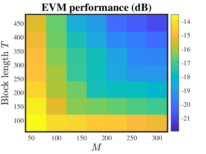
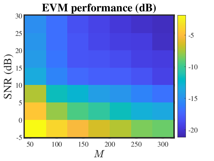
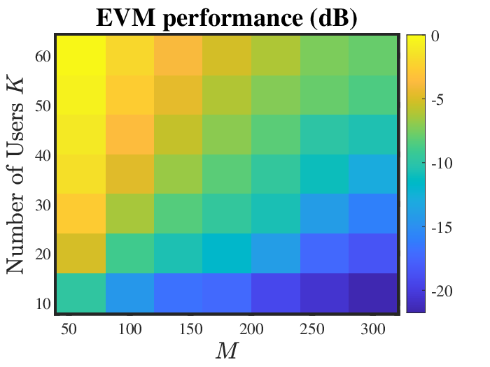
We test the impact of key system parameters on the performance of the proposed scheme with and , averaging over Monte Carlo trials. We set , , with variance and . Fig. 10(a) shows the EVM performance with dB. We see that a larger leads to a better performance since concentrates closer to the Stiefel manifold as increases, according to Proposition 1. The influence of the SNR with is given in Fig. 10(b). As it can be seen, for a fixed number of , a higher SNR leads to better performance and a large makes recovery in the low SNR region possible. These observations verify the results in Theorem 6. The influence of the number of users is given in Fig. 10(c). We see that a smaller leads to better performance which is consistent with Theorem 6.
V-B3 EVM performance with different large-scale fading
Fig.11 shows the EVM performance with and different large-scale fading among users. The large-scale fading of the -th user is generated by (dB) according to [46, Table 4], where is the 3D distance between the -th user and the BS, which is randomly drawn from , GHz, and . and is generated as the white Gaussian noise with variance , and . Though the power leakage is more severe when , the results show the robustness of the proposed scheme with large receive antenna arrays.

VI Conclusions
In this paper, we proposed to exploit the sparsity of the massive MIMO channel and the data concentration for blind data detection. An -norm maximization problem was proposed, along with theoretical justification. A parameter-free algorithm was then proposed to solve the problem with a convergence guarantee. Numerical-simulation-based results were provided to verify the correctness of the derived theorems, as well as, to demonstrate the superior performance and robustness of the proposed blind data detection method. It will be useful to develop a stochastic version for the proposed scheme to further reduce the complexity and facilitate the implementation in the large-scale OFDM mmWave systems.
-A Proof of Proposition 1
Since any bounded random variable is sub-Gaussian with , where is the sub-Gaussian norm defined as [47], and has independent, mean-zero, sub-Gaussian isotropic random columns, i.e., . Then, for any , we obtain
| (23) | ||||
where . Let , and then . Since , we have . The last inequality follows [47, Theorem 4.6.1].
-B Proof of Theorem 5
Let , and we have
| (24) | ||||
where we denote and . Using the rotation-invariant property of Guassian random variables, we have with calculated by the 3rd-order non-central moment of the Rayleigh distribution. Since , we have . The equality holds if and only if for all , which is only satisfied at [29]. Therefore, we have . Furthermore, if and , then . However, . This indicates that two different columns of cannot simultaneously equal the same standard basis vector. Hence, achieves the maximum when with .
Using the result in [32, Theorem 2.1] for the Stiefel manifold, we conclude that there exists a constant , for any , such that, whenever, .
-C Proof of Proposition 6
Let , and then we have
| (25) | ||||
where we denote and . Using the rotation invariant property of Gaussian random variables, we have with calculated by the third-order non-central moment of the Rayleigh distribution. Then, we have
| (26) | ||||
The first equality holds when and the second equality holds when .
-D Proof of Lemma 8
Define . Then, by the convexity of , we have
| (27) | ||||
where the first and second inequalities hold due to the convexity, and the last inequality holds since and , and the equality is obtained when .
-E Proof of Lemma 9
Define . Then, we have , which indicates that . That is to say, when , we have . We also have SVD, , and the stationary point of on satisfies [33]
| (28) | ||||
- •
If , we have
(29) where ;
- •
If , we have
(30)
-F Proof of Theorem 10
Define . By the convexity of , we have . By summing these inequalities for we obtain . Hence, and
-G Proof of Theorem 12
Acknowledgment
The authors would like to thank professor Yi Ma of Berkeley EECS Department for his lectures and talks at Tsinghua-Berkeley Shenzhen Institute and Yuexiang Zhai of Berkeley for stimulating discussions during preparation of this manuscript. The authors would also like to thank professor Xiaojun Yuan of UESTC to share the simulation codes and Hang Liu of CUHK for discussion on the ambiguity resolving.
References
- [1] F. Rusek, D. Persson, B. K. Lau, E. G. Larsson, T. L. Marzetta, O. Edfors, and F. Tufvesson, “Scaling up MIMO: Opportunities and challenges with very large arrays,” IEEE Signal Process. Mag., vol. 30, pp. 40–60, Jan. 2013.
- [2] X. Yu, J. Zhang, M. Haenggi, and K. B. Letaief, “Coverage analysis for millimeter wave networks: The impact of directional antenna arrays,” IEEE J. Sel. Areas Commun., vol. 35, pp. 1498–1512, July 2017.
- [3] O. Elijah, C. Y. Leow, T. A. Rahman, S. Nunoo, and S. Z. Iliya, “A comprehensive survey of pilot contamination in massive MIMO-5G system,” IEEE Commun. Surveys Tuts., vol. 18, pp. 905–923, 2nd Quart. 2016.
- [4] L. Zheng and D. N. C. Tse, “Communication on the grassmann manifold: a geometric approach to the noncoherent multiple-antenna channel,” IEEE Trans. Inf. Theory, vol. 48, pp. 359–383, Feb. 2002.
- [5] B. Muquet, M. de Courville, and P. Duhamel, “Subspace-based blind and semi-blind channel estimation for OFDM systems,” IEEE Trans. Signal Process., vol. 50, pp. 1699–1712, July 2002.
- [6] H. Q. Ngo and E. G. Larsson, “EVD-based channel estimation in multicell multiuser MIMO systems with very large antenna arrays,” in Proc. IEEE Int. Conf. Acoust. Speech and Signal Process., pp. 3249–3252, Mar. 2012.
- [7] B. Hassibi and B. M. Hochwald, “How much training is needed in multiple-antenna wireless links?,” IEEE Trans. Inf. Theory, vol. 49, no. 4, pp. 951–963, 2003.
- [8] M. K. Samimi and T. S. Rappaport, “3-D millimeter-wave statistical channel model for 5G wireless system design,” IEEE Trans. Microw. Theory Techn., vol. 64, pp. 2207–2225, July 2016.
- [9] Y. Zhou, M. Herdin, A. M. Sayeed, and E. Bonek, “Experimental study of mimo channel statistics and capacity via the virtual channel representation,” Univ. Wisconsin-Madison, Madison, WI, USA, Tech. Rep, vol. 5, pp. 10–15, 2007.
- [10] X. Rao and V. K. N. Lau, “Distributed compressive csit estimation and feedback for fdd multi-user massive MIMO systems,” IEEE Trans. Signal Process, vol. 62, no. 12, pp. 3261–3271, 2014.
- [11] J. Zhang, X. Yuan, and Y. A. Zhang, “Blind signal detection in massive MIMO: Exploiting the channel sparsity,” IEEE Trans. Commun., vol. 66, pp. 700–712, Feb. 2018.
- [12] H. Liu, X. Yuan, and Y. J. Zhang, “Super-resolution blind channel-and-signal estimation for massive MIMO with one-dimensional antenna array,” IEEE Trans. Signal Process., vol. 67, pp. 4433–4448, Sep. 2019.
- [13] A. Mezghani and A. L. Swindlehurst, “Blind estimation of sparse broadband massive MIMO channels with ideal and one-bit ADCs,” IEEE Trans. Signal Process., vol. 66, pp. 2972–2983, June 2018.
- [14] K. Ghavami and M. Naraghi-Pour, “Blind channel estimation and symbol detection for multi-cell massive MIMO systems by expectation propagation,” IEEE Trans. Wireless Commun., vol. 17, no. 2, pp. 943–954, 2018.
- [15] M. Talagrand, “A new look at independence,” Ann. Probab., vol. 24, pp. 1–34, Jan. 1996.
- [16] E. Candès and J. Romberg, “Sparsity and incoherence in compressive sampling,” Inverse Problems, vol. 23, pp. 969–985, Apr. 2007.
- [17] Q. Qu, J. Sun, and J. Wright, “Finding a sparse vector in a subspace: Linear sparsity using alternating directions,” in Proc. Adv. Neural Inf. Process. Syst., pp. 3401–3409, Dec. 2014.
- [18] Y. Zhai, Z. Yang, Z. Liao, J. Wright, and Y. Ma, “Complete dictionary learning via l4-norm maximization over the orthogonal group,” Journal of Machine Learning Research, vol. 21, no. 165, pp. 1–68, 2020.
- [19] Q. Qu, Y. Zhai, X. Li, Y. Zhang, and Z. Zhu, “Geometric analysis of nonconvex optimization landscapes for overcomplete learning,” in Proc. Int. Conf. Learn. Represent., Apr. 2020.
- [20] Y. Zhang, H. Kuo, and J. Wright, “Structured local optima in sparse blind deconvolution,” IEEE Trans. Inf. Theory, vol. 66, pp. 419–452, Jan. 2020.
- [21] Y. Li and Y. Bresler, “Global geometry of multichannel sparse blind deconvolution on the sphere,” in Proc. Adv. Neural Inf. Process. Syst., pp. 1132–1143, Dec. 2018.
- [22] O. E. Ayach, S. Rajagopal, S. Abu-Surra, Z. Pi, and R. W. Heath, “Spatially sparse precoding in millimeter wave MIMO systems,” IEEE Trans. Wireless Commun., vol. 13, pp. 1499–1513, Mar. 2014.
- [23] C. A. Balanis, Antenna Theory: Analysis and Design. USA: Wiley-Interscience, 2005.
- [24] J. Brady and A. Sayeed, “Beamspace MU-MIMO for high-density gigabit small cell access at millimeter-wave frequencies,” in Proc. IEEE Int. Workshop Signal Process. Adv. Wireless Commun., pp. 80–84, June 2014.
- [25] A. M. Sayeed, “Deconstructing multiantenna fading channels,” IEEE Trans. Signal Process., vol. 50, pp. 2563–2579, Oct. 2002.
- [26] A. L. Swindlehurst, E. Ayanoglu, P. Heydari, and F. Capolino, “Millimeter-wave massive MIMO: the next wireless revolution?,” IEEE Commun. Mag., vol. 52, pp. 56–62, Sep. 2014.
- [27] Y. Ding and B. D. Rao, “Dictionary learning-based sparse channel representation and estimation for FDD massive MIMO systems,” IEEE Trans. Wireless Commun., vol. 17, pp. 5437–5451, Aug. 2018.
- [28] S. M. Ross, A First Course in Probability. Upper Saddle River, N.J.: Prentice Hall, fifth ed., 1998.
- [29] Y. Bai, Q. Jiang, and J. Sun, “Subgradient descent learns orthogonal dictionaries,” in Proc. Int. Conf. Learn. Represent., May 2019.
- [30] J. Sun, Q. Qu, and J. Wright, “Complete dictionary recovery over the sphere I: Overview and the geometric picture,” IEEE Trans. Inf. Theory, vol. 63, pp. 853–884, Feb. 2017.
- [31] J. Sun, Q. Qu, and J. Wright, “Complete dictionary recovery over the sphere II: Recovery by riemannian trust-region method,” IEEE Trans. Inf. Theory, vol. 63, pp. 885–914, Feb. 2017.
- [32] Y. Shen, Y. Xue, J. Zhang, K. B. Letaief, and V. Lau, “Complete dictionary learning via -norm maximization,” In Proc. the 36th Conference on Uncertainty in Artificial Intelligence (UAI), PMLR volume 124., 2020.
- [33] P. A. Absil, R. Mahony, and R. Sepulchre, Optimization Algorithms on Matrix Manifolds. USA: Princeton University Press, 2007.
- [34] M. Jaggi, “Revisiting Frank-Wolfe: Projection-free sparse convex optimization,” in Proc. Int. Conf. Mach. Learn., vol. 28, pp. 427–435, PMLR, June 2013.
- [35] P.-A. Absil and J. Malick, “Projection-like retractions on matrix manifolds,” SIAM J. on Optimization, vol. 22, pp. 135–158, Jan. 2012.
- [36] J. Casey and P. M. Naghdi, “On the use of invariance requirements for intermediate configurations associated with the polar decomposition of a deformation gradient,” Quart. Applied Math., vol. 41, no. 3, pp. 339–342, 1983.
- [37] N. J. Higham and P. Papadimitriou, “A parallel algorithm for computing the polar decomposition,” Parallel Comput., vol. 20, pp. 1161–1173, Aug. 1994.
- [38] R. Hunger, Floating point operations in matrix-vector calculus. Munich University of Technology, Inst. for Circuit Theory and Signal Process., 2005.
- [39] S. Alameddin, A. Fau, D. Néron, P. Ladevèze, and U. Nackenhorst, “Toward optimality of proper generalised decomposition bases,” Mathematical and Computational Applications, vol. 24, no. 1, p. 30, 2019.
- [40] J. P. Vila and P. Schniter, “Expectation-maximization gaussian-mixture approximate message passing,” IEEE Trans. Signal Process., vol. 61, pp. 4658–4672, Oct. 2013.
- [41] X. Li, S. Chen, Z. Deng, Q. Qu, Z. Zhu, and A. M. C. So, “Nonsmooth optimization over Stiefel manifold: Riemannian subgradient methods,” arXiv preprint arXiv:1911.05047, 2019.
- [42] G. Destino, M. Juntti, and S. Nagaraj, “Leveraging sparsity into massive MIMO channel estimation with the adaptive-LASSO,” in Proc. IEEE Global Conf. Signal Inf. Process., pp. 166–170, Dec. 2015.
- [43] S. Boyd, N. Parikh, E. Chu, B. Peleato, and J. Eckstein, Distributed Optimization and Statistical Learning via the Alternating Direction Method of Multipliers. 2011.
- [44] Q. Qu, X. Li, and Z. Zhu, “A nonconvex approach for exact and efficient multichannel sparse blind deconvolution,” in Proc. Adv. Neural Inf. Process. Syst., pp. 4017–4028, Dec. 2019.
- [45] X. Kuai, X. Yuan, W. Yan, H. Liu, and Y. J. Zhang, “Double-sparsity learning based channel-and-signal estimation in massive MIMO with generalized spatial modulation,” IEEE Trans. Wireless Commun., 2020.
- [46] T. S. Rappaport, Y. Xing, G. R. MacCartney, A. F. Molisch, E. Mellios, and J. Zhang, “Overview of millimeter wave communications for fifth-generation (5G) wireless networks with a focus on propagation models,” IEEE Trans. Antennas Propag., vol. 65, pp. 6213–6230, Dec. 2017.
- [47] R. Vershynin, High-Dimensional Probability: An Introduction with Applications in Data Science. Cambridge University Press, 2018.