Convex Representation Learning for Generalized Invariance in
Semi-Inner-Product Space
Abstract
Invariance (defined in a general sense) has been one of the most effective priors for representation learning. Direct factorization of parametric models is feasible only for a small range of invariances, while regularization approaches, despite improved generality, lead to nonconvex optimization. In this work, we develop a convex representation learning algorithm for a variety of generalized invariances that can be modeled as semi-norms. Novel Euclidean embeddings are introduced for kernel representers in a semi-inner-product space, and approximation bounds are established. This allows invariant representations to be learned efficiently and effectively as confirmed in our experiments, along with accurate predictions.
1 Introduction
Effective modeling of structural priors has been the workhorse of a variety of machine learning algorithms. Such priors are available in a rich supply, including invariance (Simard et al. 1996; Ferraro and Caelli 1994), equivariance (Cohen and Welling 2016; Graham and Ravanbakhsh 2019), disentanglement (Bengio et al. 2013; Higgins et al. 2017), homophily/heterophily (Eliassi-Rad and Faloutsos 2012), fairness (Creager et al. 2019), correlations in multiple views and modalities (Wang et al. 2015; Kumar et al. 2018), etc.
In this paper we focus on “generalized invariance”, where certain relationship holds irrespective of certain changes in data. This extends traditional settings that are limited to, e.g., transformation and permutation. For instance, in multilabel classification there are semantic or logical relationships between classes which hold for any input. Common examples include mutual exclusion and implication (Mirzazadeh et al. 2015a; Deng et al. 2012). In mixup (Zhang et al. 2018), a convex interpolation of a pair of examples is postulated to yield the same interpolation of output labels.
While conventional wisdom learns models whose prediction accords with these structures, recent developments show that it can be more effective to learn structure-encoding representations. Towards this goal, the most straightforward approach is to directly parameterize the model. For example, deep sets model permutation invariance via an additive decomposition (Zaheer et al. 2017), convolutional networks use sparse connection and parameter sharing to model translational invariance, and a similar approach has been developed for equivariance (Ravanbakhsh et al. 2017). Although they simplify the model and can enforce invariance over the entire space, their applicability is very restricted, because most useful structures do not admit a readily decomposable parameterization. As a result, most invariance/equivariance models are restricted to permutations and group based diffeomorphism.
In order to achieve significantly improved generality and flexibility, the regularization approach can be leveraged, which penalizes the violation of pre-specified structures. For example, Rifai et al. 2011 penalizes the norm of the Jacobian matrix to enforce contractivity, conceivably a generalized type of invariance. Smola 2019 proposed using a max-margin loss over all transformations (Teo et al. 2007). However, for most structures, regularization leads to a nonconvex problem. Despite the recent progress in optimization for deep learning, the process still requires a lot of trial and error. Therefore a convex learning procedure will be desirable, because besides the convenience in optimization, it also offers the profound advantage of decoupling parameter optimization from problem specification: poor learning performance can only be ascribed to a poor model architecture, not to poor local minima.
Indeed convex invariant representation learning has been studied, but in limited settings. Tangent distance kernels (Haasdonk and Keysers 2002) and Haar integration kernels are engineered to be invariant to a group of transformations (Raj et al. 2017; Mroueh et al. 2015; Haasdonk and Burkhardt 2007), but it relies on sampling for tractable computation and the sample complexity is where is the dimension of the underlying space. Bhattacharyya et al. 2005 treated all perturbations within an ellipsoid neighborhood as invariances, and it led to an expensive second order cone program (SOCP). Other distributionally robust formulations also lead to SOCP/SDPs (Rahimian and Mehrotra 2019). The most related work is Ma et al. 2019, which warped a reproducing kernel Hilbert space (RKHS) by linear functionals that encode the invariances. However, in order to keep the warped space an RKHS, their applicability is restricted to quadratic losses on linear functionals.
In practice, however, there are many invariances that cannot be modeled by quadratic penalties. For example, the logical relationships between classes impose an ordering in the discriminative output (Mirzazadeh et al. 2015a), and this can hardly be captured by quadratic forms. Similarly, when a large or infinite number of invariances are available, measuring the maximum violation makes more sense than their sum, and it is indeed the principle underlying adversarial learning (Madry et al. 2018). Again this is not amenable to quadratic forms.
Our goal, therefore, is to develop a convex representation learning approach that efficiently incorporates generalized invariances as semi-norm functionals. Our first contribution is to show that compared with linear functionals, semi-norm functionals encompass a much broader range of invariance (Sections 5 and 6).
Our key tool is the semi-inner-product space (Lumer 1961, s.i.p.,), into which an RKHS can be warped by augmenting the RKHS norm with semi-norm functionals. A specific example of s.i.p. space is the reproducing kernel Banach space (Zhang et al. 2009), which has been used for regularization in, e.g., kernel SVMs, and suffers from high computational cost (Salzo et al. 2018; Der and Lee 2007; Bennett and Bredensteiner 2000; Hein et al. 2005; von Luxburg and Bousquet 2004; Zhou et al. 2002). A s.i.p. space extends RKHS by relaxing the underlying inner product into a semi-inner-product, while retaining the important construct: kernel function. To our best knowledge, s.i.p. space has yet been applied to representation learning.
Secondly, we developed efficient computation algorithms for solving the regularized risk minimization (RRM) with the new s.i.p. norm (Section 3). Although Zhang et al. 2009 established the representer theorem from a pure mathematical perspective, no practical algorithm was provided and ours is the first to fill this gap.
However, even with this progress, RRMs still do not provide invariant representations of data instances; it simply learns a discriminant function by leveraging the representer theorem (which does hold in the applications we consider). So our third contribution, as presented in Section 4, is to learn and extract representations by embedding s.i.p. kernel representers in Euclidean spaces. This is accomplished in a convex and efficient fashion, constituting a secondary advantage over RRMs which is not convex in the dual coefficients. Different from Nyström or Fourier linearization of kernels in RKHS, the kernel representers in a s.i.p. space carry interestingly different meanings and expressions in primal and dual spaces. Finally, our experiments demonstrate that the new s.i.p.-based algorithm learns more predictive representations than strong baselines.
2 Preliminaries
Suppose we have an RKHS with , inner product and kernel . Our goal is to renorm hence warp the distance metric by adding a functional that induces desired structures.
2.1 Existing works on invariance modeling by RKHS
Smola and Schölkopf 1998 and Zhang et al. 2013 proposed modeling invariances by bounded linear functionals in RKHS. Given a function , the graph Laplacian is , and obviously is bounded and linear. Transformation invariance can be characterized by , where stands for the image after applying an amount of rotation, translation, etc. It is again bounded and linear. By Riesz representation theorem, a bounded linear functional can be written as for some .
Based on this view, Ma et al. 2019 took a step towards representation learning. By adding to the RKHS norm square, the space is warped to favor that respects invariance, i.e., small magnitude of . They showed that it leads to a new RKHS with a kernel
| (1) |
where and .
Although the kernel representer of offers a new invariance aware representation, the requirement that the resulting space remains an RKHS forces the penalties in to be quadratic on , significantly limiting its applicability to a broader range of invariances such as total variation . Our goal is to relax this restriction by enabling semi-norm regularizers with new tools in functional analysis, and illustrate its applications in Sections 5 and 6.
2.2 Semi-inner-product spaces
We first specify the range of regularizer considered here.
Assumption 1.
We assume that is a semi-norm. Equivalently, is convex and for all and (absolute homogeneity). Furthermore, we assume is closed (i.e., lower semicontinuous) w.r.t. the topology in .
Since is closed convex and its domain is the entire Hilbert space , must be continuous. By exempting from being induced by an inner product, we enjoy substantially improved flexibility in modeling various regularities.
For most learning tasks addressed below, it will be convenient to directly construct from the specific regularity. However, in some context it will also be convenient to constructively explicate in terms of support functions.
Proposition 1.
satisfies Assumption 1 if, and only if, , where is bounded in the RKHS norm and is symmetric ().
The proof is in Appendix A. Using , we arrive at a new norm defined by
| (2) |
thanks to Assumption 1. It is immediately clear from Proposition 1 that , for some constant that bounds the norm of . In other words, the two norms and are equivalent, hence in particular the norm is complete. We thus arrive at a Banach space . Note that both and have the same underlying vector space —the difference is in the norm or distance metric. To proceed, we need to endow more structures on .
Definition 1 (Strict convexity).
A normed vector space is strictly convex if for all ,
| (3) |
implies for some . Equivalently, if the unit ball is strictly convex.
Using the parallelogram law it is clear that the Hilbert norm is strictly convex. Moreover, since summation preserves strict convexity, it follows that the new norm is strictly convex as well.
Definition 2 (Gâteaux differentiability).
A normed vector space is Gâteaux differentiable if for all , there exists the directional derivative
| (4) |
We remark that both strict convexity and Gâteaux differentiability are algebraic but not topological properties of the norm. In other words, two equivalent (in terms of topology) norms may not be strictly convex or Gâteaux differentiable at the same time. For instance, the -norm on is both strictly convex and Gâteaux differentiable, while the equivalent -norm is not.
Recall that is the dual space of , consisting of all continuous linear functionals on and equipped with the dual norm . The dual space of a normed (reflexive) space is Banach (reflexive).
Definition 3.
A Banach space is reflexive if the canonical map , is onto, where is the (bilinear) duality pairing between dual spaces. Here is any element in .
Note that reflexivity is a topological property. In particular, equivalent norms are all reflexive if any one of them is. As any Hilbert space is reflexive, so is the equivalent norm in (2).
Theorem 1 (Borwein and Vanderwerff 2010).
A Banach space is strictly convex (Gâteaux differentiable) if its dual space is Gâteaux differentiable (strictly convex). The converse is true too if is reflexive.
Combining Proposition 1 and Theorem 1, we see that , hence , is Gâteaux differentiable if (the closed convex hull of) the set in Proposition 1 is strictly convex.
We are now ready to define a semi-inner-product (s.i.p.) on a normed space . We call a bivariate mapping a s.i.p. if for all and ,
- •
additivity:
- •
homogeneity: ,
- •
norm-inducing: ,
- •
Cauchy-Schwarz: .
We note that an s.i.p. is additive in its second argument iff it is an inner product (by simply verifying the parellelogram law). Lumer 1961 proved that s.i.p. does exist on every normed space. Indeed, let the subdifferential be the (multi-valued) duality mapping. Then, any selection with the convention that leads to a s.i.p.:
| (5) |
Indeed, from definition, for any , , where and . A celebrated result due to Giles 1967 revealed the uniqueness of s.i.p. if the norm is Gâteaux differentiable, and later Faulkner 1977 proved that the (unique) mapping is onto iff is reflexive. Moreover, is 1-1 if is strictly convex (like in (2)), as was shown originally in Giles 1967.
Let us summarize the above results.
Definition 4.
A Banach space is called a s.i.p. space iff it is reflexive, strictly convex, and Gâteaux differentiable. Clearly, the dual of a s.i.p. space is s.i.p. too.
Theorem 2 (Riesz representation).
Let be a s.i.p. space. Then, for any continuous linear functional , there exists a unique such that
| (6) |
From now on, we identify the duality mapping with the star operator . Thus, we have a unique way to represent all continuous functionals on a s.i.p. space. Conveniently, the unique s.i.p. on the dual space follows from (5): for all ,
| (7) |
from which one easily verifies all properties of an s.i.p. Some literature writes , , , and to explicitize where the operations take place. We simplify these notations by omitting subscripts when the context is clear, but still write and .
Finally, fix and consider the evaluation (linear) functional , . When is continuous (which indeed holds for our norm (2)), Theorem 2 implies the existence of a unique such that
| (8) |
Varying we obtain a unique s.i.p. kernel such that . Thus, using s.i.p. we obtain the reproducing property:
| (9) |
Different from a reproducing kernel in RKHS, is not necessarily symmetric or positive semi-definite.
3 Regularized Risk Minimization
In this section we aim to provide a computational device for the following regularized risk minimization (RRM) problem:
| (10) |
where is the empirical risk depending on discriminant function values for training examples . Clearly, this objective is equivalent to
| (11) |
Remark 1.
Unlike the usual treatment in reproducing kernel Banach spaces (RKBS) (Zhang et al. 2009, e.g.), we only require to be reflexive, strictly convex and Gâteaux differentiable, instead of the much more demanding uniform convexity and smoothness. This more general condition not only suffices for our subsequent results but also simplifies the presentation. A similar definition like ours was termed pre-RKBS in Combettes et al. 2018.
Zhang et al. 2009 established the representer theorem for RKBS: the optimal for (11) has its dual form
| (12) |
where are real coefficients. To optimize , we need to substitute (12) into (11), which in turn requires evaluating i) , which equals ; ii) , which, can be computed through inverting the star operator as follows:
where the last equality is due to (8) and (5). The last maximization step operates in the RKHS , and thanks to the strict convexity of , it admits the unique solution
| (13) |
because , and is a s.i.p. space.
We summarize this computational inverse below:
Theorem 3.
In practice, we first compute by solving (14), and then can be evaluated at different without redoing any optimization. As a special case, setting allows us to evaluate the kernel .
Specialization to RKHS.
When , is induced by an inner product, making an RKHS. Now we can easily recover (1) by applying Theorem 3, because the optimization in (14) with is
| (16) |
and its unique solution can be easily found in closed form:
| (17) |
Plugging into , we recover (1).
Overall, the optimization of (11) may no longer be convex in , because is generally not linear in even though is (since the star operator is not linear). In practice, we can initialize by training without (i.e., setting to 0). Despite the nonconvexity, we have achieved a new solution technique for a broad class of inverse problems, where the regularizer is a semi-norm.
4 Convex Representation Learning by Euclidean Embedding
Interestingly, our framework—which so far only learns a predictive model—can be directly extended to learn structured representations in a convex fashion. In representation learning, one identifies an “object” for each example , which, in our case, can be a function in or a vector in Euclidean space. Such a representation is supposed to have incorporated the prior invariances in , and can be directly used for other (new) tasks such as supervised learning without further regularizing by . This is different from the RRM in Section 3, which, although still enjoys the representer theorem in the applications we consider, only seeks a discriminant function without providing a new representation for each example.
Our approach to convex representation learning is based on Euclidean embeddings (a.k.a. finite approximation or linearization) of the kernel representers in a s.i.p. space, which is analogous to the use of RKHS in extracting useful features. However, different from RKHS, and play different roles in a s.i.p. space, hence require different embeddings in . For any and , we will seek their Euclidean embeddings and , respectively. Note is just a notation, not to be interpreted as “the adjoint of .”
We start by identifying the properties that a reasonable Euclidean embedding should satisfy intuitively. Motivated by the bilinearity of , it is natural to require
| (18) |
where stands for Euclidean inner product. As is bilinear, and should be linear on and respectively. Also note in general.
Similar to the linearization of RKHS kernels, we can apply invertible transformations to and . For example, doubling while halving makes no difference. We will just choose one representation out of them. It is also noteworthy that in general, (Euclidean norm) approximates instead of . (18) is the only property that our Euclidean embedding needs to satisfy.
We start by embedding the unit ball . Characterizing by support functions as in Proposition 1, a natural Euclidean approximation of is
| (19) |
where is the Euclidean embedding of in the original RKHS, designed to satisfy that for all (or a subset of interest). Commonly used embeddings include Fourier (Rahimi and Recht 2008), hash (Shi et al. 2009), Nyström (Williams and Seeger 2000), etc. For example, given landmarks sampled from , the Nyström approximation for a function is
| (20) | ||||
| (21) |
Naturally, the dual norm of is
| (22) |
Clearly the unit ball of and are also symmetric, and we denote them as and , respectively.
As shown in Figure 1, we have the following commutative diagram. Let be the star operator and its inverse, and similarly for and its inverse . Then, it is natural to require
| (23) |
where can be computed for any via a Euclidean counterpart of Theorem 3:
| (24) |
The argmax is unique because is strictly convex.
At last, how can we get in the first place? We start from the simpler case where has a kernel expansion as in (12).11 1 We stress that although the kernel expansion (12) is leveraged to motivate the design of , the underpinning foundation is that the span of is dense in (Theorem 4). The representer theorem (Zhang et al. 2009, Theorem 2), which showed that the solution to (11) must be in the form of (12), is not relevant to our construction. Here, by the linearity of , it will suffice to compute . By Theorem 3,
is uniquely attained. Denoting , it follows
So by comparing with (18), it is natural to introduce
| (25) | ||||
| (26) | ||||
| (27) |
The last optimization is convex and can be solved very efficiently because, thanks to the positive homogeneity of , it is equivalent to
| (28) |
Detailed derivation and proof are relegated to Appendix C. To solve (28), LBFGS with projection to a hyperplane (which has a trivial closed-form solution) turned out to be very efficient in our experiment. Overall, the construction of and for from (12) proceeds as follows:
- 1.
Define ;
- 2.
Define for ;
- 3.
Define based on by using (23).
In the next subsection, we will show that these definitions are sound, and both and are linear. However, the procedure may still be inconvenient in computation, because needs to be first dualized to , which in turn needs to be expanded into the form of (12). Fortunately, our representation learning only needs to compute the embedding of , bypassing all these computational challenges.
4.1 Analysis of Euclidean Embeddings
The previous derivations are based on the necessary conditions for (18) to hold. We now show that and are well-defined, and are linear. To start with, denote the base Euclidean embedding on by , where . Then by assumption, is linear and .
Theorem 4.
is well defined for all , and is linear. That is,
- a)
If are two different expansions of , then .
- b)
The linear span of is dense in . So extending the above to the whole is straightforward thanks to the linearity of .
We next analyze the linearity of . To start with, we make two assumptions on the Euclidean embedding of .
Assumption 2 (surjectivity).
For all , there exists a such that .
Assumption 2 does not cost any generality, because it is satisfied whenever the coordinates of the embedding are linearly independent. Otherwise, this can still be enforced easily by projecting to an orthonormal basis of .
Assumption 3 (lossless).
for all . This is possible when, e.g., is finite dimensional.
4.2 Analysis under Inexact Euclidean Embedding
When Assumption 3 is unavailable, Theorem 4 still holds, but the linearity of has to be relaxed to an approximate sense. To analyze it, we first rigorously quantify the inexactness of the Euclidean embedding . Consider a subspace based embedding, such as Nyström approximation. Here satisfies that there exists a countable set of orthonormal bases of , such that
- 1.
for all ,
- 2.
, .
Clearly the Nyström approximation in (20) satisfies these conditions, where , and is any orthornormal basis of (assuming is no more than the dimensionality of ).
Definition 5.
is called -approximable by if
| (29) |
In other words, the component of in is at most .
Theorem 6 (The proof is in Appendix B).
Let and . Then . If , , and all elements in are -approximable by , then
| (30) | ||||
| (31) |
To summarize, the primal embedding as defined in (26) provides a new feature representation that incorporates structures in the data. Based on it, a simple linear model can be trained to achieve the desired regularities in prediction. We now demonstrate its flexibility and effectiveness on two example applications.
5 Application 1: Mixup
Mixup is a data augmentation technique (Zhang et al. 2018), where a pair of training examples and are randomly selected, and their convex interpolation is postulated to yield the same interpolation of output labels. In particular, when is the one-hot vector encoding the class that belongs to, the loss for the pair is
| (32) |
Existing literature relies on stochastic optimization, with a probability pre-specified on . This is somewhat artificial. Changing expectation to maximization appears more appealing, but no longer amenable to stochastic optimization.
To address this issue and to learn representations that incorporate mixup prior while also accommodating classification with multiclass or even structured output, we resort to a joint kernel , whose simplest form is decomposed as . Here and are separate kernels on input and output respectively. Now a function learned from the corresponding RKHS quantifies the “compatibility” between and , and the prediction can be made by . In this setting, the for mixup regularization can leverage the norm of over , effectively accounting for an infinite number of invariances.
Clearly taking expectation or maximization over all pairs of training examples still satisfies Assumption 1. In our experiment, we will use the norm, which despite not being covered by Theorem 7, is directly amenable to the embedding algorithm. More specifically, for each pair we need to embed as a matrix. This is different from the conventional setting where each example employs one feature representation shared for all classes; here the representation changes for different classes . To this end, we need to first embed each invariance by
Letting and , the Euclidean embedding can be derived by solving (28):
| (33) | ||||
| (34) |
Although the maximization over in (33) is not concave, it is 1-D and a grid style search can solve it globally with complexity. In practice, a local solver like L-BFGS almost always found its global optimum in 10 iterations.
6 Application 2: Embedding Inference for Structured Multilabel Prediction
In output space, there is often prior knowledge about pairwise or multi-way relationships between labels/classes. For example, if an image represents a cat, then it must represent an animal, but not a dog (assuming there is at most one object in an image). Such logic relationships of implication and exclusion can be highly useful priors for learning (Mirzazadeh et al. 2015a; Deng et al. 2012). One way to leverage it is to perform inference at test time so that the predicted multilabel conforms to these logic. However, this can be computation intensive at test time, and it will be ideal if the predictor has already accounted for these logic, and at test time, one just needs to make binary decisions (relevant/irrelevant) for each individual category separately. We aim to achieve this by learning a representation that embeds this structured prior.
To this end, it is natural to employ the joint kernel framework. We model the implication relationship of by enforcing , which translates to a penalty on the amount by which is above
| (35) |
To model the mutual exclusion relationship of , intuitively we can encourage that , i.e., a higher likelihood of being a cat demotes the likelihood of being a dog. It also allows both and to be irrelevant, i.e., both and are negative. This amounts to another sublinear penalty on : . To summarize, letting be the empirical distribution, we can define by
| (36) | ||||
| (37) |
It is noteworthy that although is positively homogeneous and convex (hence sublinear), it is no longer absolutely homogeneous and therefore not satisfying Assumption 1. However, the embedding algorithm is still applicable without change. It will be interesting to study the presence of kernel function in spaces “normed” by sublinear functions. We leave it for future work.
7 Experiments
Here we highlight the major results and experiment setup. Details on data preprocessing, experiment setting, optimization, and additional results are given in Appendix E.
7.1 Sanity check for s.i.p. based methods
Our first experiment tries to test the effectiveness of optimizing the regularized risk (11) with respect to the dual coefficients in (12). We compared 4 algorithms: SVM with Gaussian kernel; Warping which incorporates transformation invariance by kernel warping as described in Ma et al. 2019; Dual which trains the dual coefficients by LBFGS to minimize empirical risk as in (11); Embed which finds the Euclidean embeddings by convex optimization as in (28), followed by a linear classifier. The detailed derivation of the gradient in for Dual is relegated to Appendix D.
| SVM | Warping | Dual | Embed | |
|---|---|---|---|---|
| 4 v.s. 9 | 97.1 | 98.0 | 97.6 | 97.8 |
| 2 v.s. 3 | 98.4 | 99.1 | 98.7 | 98.9 |
Four transformation invariances were considered, including rotation, scaling, and shifts to the left and upwards. Warping summed up the square of over the four transformations, while Dual and Embed took their max as the . To ease the computation of derivative, we resorted to finite difference for all methods, with two pixels for shifting, 10 degrees for rotation, and 0.1 unit for scaling. No data augmentation was applied.
All algorithms were evaluated on two binary classification tasks: 4 v.s. 9 and 2 v.s. 3, both sampling 1000 training and 1000 test examples from the MNIST dataset.
Since the square loss on the invariances used by Warping makes good sense, the purpose of this experiment is not to show that the s.i.p. based methods are better in this setting. Instead we aim to perform a sanity check on a) good solutions can be found for the nonconvex optimization over the dual variables in Dual, b) the Euclidean embedding of s.i.p. representers performs competitively. As Table 1 shows, both checks turned out affirmative, with Dual and Embed delivering similar accuracy as Warping. In addition, Embed achieved higher accuracy than dual optimization, suggesting that the learned representations have well captured the invariances and possess better predictive power.
7.2 Mixup
We next investigated the performance of Embed on mixup.
| Dataset | |||||||
|---|---|---|---|---|---|---|---|
| MNIST | Vanilla | ||||||
| Embed | |||||||
| USPS | Vanilla | ||||||
| Embed | |||||||
| Fashion MNIST | Vanilla | ||||||
| Embed | |||||||
| Dataset | Embed | ML-SVM | HR-SVM | ||||||
|---|---|---|---|---|---|---|---|---|---|
| Enron | |||||||||
| Reuters | |||||||||
| WIPO | |||||||||
Datasets.
We experimented with three image datasets: MNIST, USPS, and Fashion MNIST, each containing 10 classes. From each dataset, we drew examples for training and examples for testing. Based on the training data, number of pairs were drawn from it.
Both Vanilla and Embed used Gaussian RKHS, along with Nyström approximation whose landmark points consisted of the entire training set. The vanilla mixup optimizes the objective (32) averaged over all sampled pairs. Following Zhang et al. 2018, The was generated from a Beta distribution, whose parameter was tuned to optimize the performance. Again, Embed was trained with a linear classifier.
Algorithms.
We first ran mixup with stochastic optimization where pairs were drawn on the fly. Then we switched to batch training of mixup (denoted as Vanilla), with the number of sampled pair increased from , , up to . It turned out when , the performance already matches the best test accuracy of the online stochastic version, which generally witnesses much more pairs. Therefore we also varied in when training Embed. each setting was evaluated 10 times with randomly sampled training and test data. The mean and standard deviation are reported in Table 3.
Results.
As Table 3 shows, Embed achieves higher accuracy than Vanilla on almost all datasets and combinations of and . The margin tends to be higher when the training set size ( and ) is smaller. Besides, Vanilla achieves the highest accuracy at .
7.3 Structured multilabel prediction
Finally, we validate the performance of Embed on structured multilabel prediction as described in Section 6, showing that it is able to capture the structured relationships between the class labels (implication and exclusion) in a hierarchical multilabel prediction task.
Datasets.
We conducted experiments on three multilabel datasets where additional information is available about the hierarchy in its class labels (link): Enron (Klimt and Yang 2004), WIPO (Rousu et al. 2006), Reuters (Lewis et al. 2004). Implication constraints were trivially derived from the hierarchy, and we took siblings (of the same parent) as exclusion constraints. For each dataset, we experimented with randomly drawn train/test examples.
Algorithms.
We compared Embed with two baseline algorithms for multilabel classification: a multilabel SVM with RBF kernel (ML-SVM), and an SVM that incorporates the hierarchical label constraints (HR-SVM) (Vateekul et al. 2012). No inference is conducted at test time, such as removing violations of implications or exclusions known a priori.
Results.
Table 3 reports the accuracy on the three train/test splits for each of the datasets. Clearly, Embed outperforms both the baselines in most of the cases.
8 Conclusions and Future Work
In this paper, we introduced a new framework of representation learning where an RKHS is turned into a semi-inner-product space via a semi-norm regularizer, broadening the applicability of kernel warping to generalized invariances, i.e., relationships that hold irrespective of certain changes in data. For example, the mixup regularizer enforces smooth variation irrespective of the interpolation parameter , and the structured multilabel regularizer enforces logic relationships between labels regardless of input features. Neither of them can be modeled convexly by conventional methods in transformation invariance, and the framework can also be directly applied to non-parametric transformations (Pal et al. 2017). An efficient Euclidean embedding algorithm was designed and its theoretical properties are analyzed. Favorable experimental results were demonstrated for the above two applications.
This new framework has considerable potential of being applied to other invariances and learning scenarios. For example, it can be directly used in maximum mean discrepancy and the Hilbert–Schmidt independence criterion, providing efficient algorithms that complement the mathematical analysis in Fukumizu et al. 2011. It can also be applied to convex deep neural networks (Ganapathiraman et al. 2018; Ganapathiraman et al. 2016), which convexify multi-layer neural networks through kernel matrices of the hidden layer outputs.
Other examples of generalized invariance include convex learning of: a) node representations in large networks that are robust to topological perturbations (Zügner et al. 2018). The exponential number of perturbation necessitates max instead of sum; b) equivariance based on the largest deviation under swapped transformations over the input domain (Ravanbakhsh et al. 2017); and c) co-embedding multiway relations that preserve co-occurrence and affinity between groups (Mirzazadeh et al. 2015b).
Acknowledgements
We thank the reviewers for their constructive comments. This work is supported by Google Cloud and NSF grant RI:1910146. YY thanks NSERC and the Canada CIFAR AI Chairs program for funding support.
References
- Bengio et al. [2013] Y. Bengio, A. Courville, and P. Vincent. Representation learning: A review and new perspectives. IEEE Transactions on Pattern Analysis and Machine Intelligence, 35(8):1798–1828, 2013.
- Bennett and Bredensteiner [2000] K. P. Bennett and E. J. Bredensteiner. Duality and geometry in SVM classifiers. In P. Langley, editor, International Conference on Machine Learning (ICML), pages 57–64, San Francisco, California, 2000. Morgan Kaufmann Publishers.
- Bhattacharyya et al. [2005] C. Bhattacharyya, K. S. Pannagadatta, and A. J. Smola. A second order cone programming formulation for classifying missing data. In Advances in Neural Information Processing Systems (NeurIPS), pages 153–160, 2005.
- Borwein and Vanderwerff [2010] J. M. Borwein and J. D. Vanderwerff. Convex Functions: Constructions, Characterizations and Counterexamples. Cambridge University Press, 2010.
- Cohen and Welling [2016] T. S. Cohen and M. Welling. Group Equivariant Convolutional Networks. In International Conference on Machine Learning (ICML), 2016.
- Combettes et al. [2018] P. L. Combettes, S. Salzo, and S. Villa. Regularized learning scheme in feature Banach spaces. Analysis and Applications, 16(1):1–54, 2018.
- Creager et al. [2019] E. Creager, D. Madras, J.-H. Jacobsen, M. Weis, K. Swersky, T. Pitassi, and R. Zemel. Flexibly fair representation learning by disentanglement. In International Conference on Machine Learning (ICML), 2019.
- Deng et al. [2012] J. Deng, N. Ding, Y. Jia, A. Frome, K. Murphy, S. Bengio, Y. Li, H. Neven, and H. Adam. Large-scale object classification using label relation graphs. In European Conference on Computer Vision (ECCV), 2012.
- Der and Lee [2007] R. Der and D. Lee. Large-margin classification in Banach spaces. In International Conference on Artificial Intelligence and Statistics (AISTATS), 2007.
- Eliassi-Rad and Faloutsos [2012] T. Eliassi-Rad and C. Faloutsos. Discovering roles and anomalies in graphs:theory and applications. Tutorial at SIAM International Conference on Data Mining (ICDM), 2012.
- Faulkner [1977] G. D. Faulkner. Representation of linear functionals in a Banach space. Rocky Mountain Journal of Mathematics, 7(4):789–792, 1977.
- Ferraro and Caelli [1994] M. Ferraro and T. M. Caelli. Lie transformation groups, integral transforms, and invariant pattern recognition. Spatial Vision, 8:33–44, 1994.
- Fukumizu et al. [2011] K. Fukumizu, G. R. Lanckriet, and B. K. Sriperumbudur. Learning in Hilbert vs. Banach spaces: A measure embedding viewpoint. In Advances in Neural Information Processing Systems (NeurIPS), 2011.
- Ganapathiraman et al. [2016] V. Ganapathiraman, X. Zhang, Y. Yu, and J. Wen. Convex two-layer modeling with latent structure. In Advances in Neural Information Processing Systems (NeurIPS), 2016.
- Ganapathiraman et al. [2018] V. Ganapathiraman, Z. Shi, X. Zhang, and Y. Yu. Inductive two-layer modeling with parametric bregman transfer. In International Conference on Machine Learning (ICML), 2018.
- Giles [1967] J. R. Giles. Classes of semi-inner-product spaces. Transactions of the American Mathematical Society, 129(3):436–446, 1967.
- Graham and Ravanbakhsh [2019] D. Graham and S. Ravanbakhsh. Equivariant entity-relationship networks. arXiv:1903.09033, 2019.
- Haasdonk and Burkhardt [2007] B. Haasdonk and H. Burkhardt. Invariant kernel functions for pattern analysis and machine learning. Machine Learning, 68(1):35–61, 2007.
- Haasdonk and Keysers [2002] B. Haasdonk and D. Keysers. Tangent distance kernels for support vector machines. In Pattern Recognition, 2002. Proceedings. 16th International Conference on, volume 2, pages 864–868. IEEE, 2002.
- Hein et al. [2005] M. Hein, O. Bousquet, and B. Schölkopf. Maximal margin classification for metric spaces. J. Comput. System Sci., 71:333–359, 2005.
- Higgins et al. [2017] I. Higgins, L. Matthey, A. Pal, C. Burgess, X. Glorot, M. Botvinick, S. Mohamed, and A. Lerchner. -vae: Learning basic visual concepts with a constrained variational framework. In International Conference on Learning Representations (ICLR), 2017.
- Hörmander [1954] L. Hörmander. Sur la fonction d’appui des ensembles convexes dans un espace loealement convexe. Arkiv För Matematik, 3(12):181–186, 1954.
- Klimt and Yang [2004] B. Klimt and Y. Yang. The enron corpus: A new dataset for email classification research. In European Conference on Machine Learning (ECML), pages 217–226. Springer, 2004.
- Kumar et al. [2018] A. Kumar, P. Sattigeri, K. Wadhawan, L. Karlinsky, R. Feris, W. T. Freeman, and G. Wornell. Co-regularized alignment for unsupervised domain adaptation. In Advances in Neural Information Processing Systems (NeurIPS), 2018.
- Lewis et al. [2004] D. D. Lewis, Y. Yang, T. G. Rose, and F. Li. Rcv1: A new benchmark collection for text categorization research. Journal of Machine Learning Research (JMLR), 5(Apr):361–397, 2004.
- [26] link. Multilabel dataset. https://sites.google.com/site/hrsvmproject/datasets-hier.
- Lumer [1961] G. Lumer. Semi-inner-product spaces. Transactions of the American Mathematical Society, 100:29–43, 1961.
- Ma et al. [2019] Y. Ma, V. Ganapathiraman, and X. Zhang. Learning invariant representations with kernel warping. In International Conference on Artificial Intelligence and Statistics (AISTATS), 2019.
- Madry et al. [2018] A. Madry, A. Makelov, L. Schmidt, D. Tsipras, and A. Vladu. Towards deep learning models resistant to adversarial attacks. In International Conference on Learning Representations (ICLR), 2018.
- Mirzazadeh et al. [2015a] F. Mirzazadeh, S. Ravanbakhsh, N. Ding, and D. Schuurmans. Embedding inference for structured multilabel prediction. In Advances in Neural Information Processing Systems (NeurIPS), 2015a.
- Mirzazadeh et al. [2015b] F. Mirzazadeh, M. White, A. György, and D. Schuurmans. Scalable metric learning for co-embedding. In European Conference on Machine Learning (ECML), 2015b.
- Mroueh et al. [2015] Y. Mroueh, S. Voinea, and T. Poggio. Learning with group invariant features: A kernel perspective. In Advances in Neural Information Processing Systems (NeurIPS), 2015.
- Pal et al. [2017] D. K. Pal, A. A. Kannan, G. Arakalgud, and M. Savvides. Max-margin invariant features from transformed unlabeled data. In Advances in Neural Information Processing Systems (NeurIPS), 2017.
- Rahimi and Recht [2008] A. Rahimi and B. Recht. Random features for large-scale kernel machines. In J. Platt, D. Koller, Y. Singer, and S. Roweis, editors, Advances in Neural Information Processing Systems (NeurIPS). MIT Press, Cambridge, MA, 2008.
- Rahimian and Mehrotra [2019] H. Rahimian and S. Mehrotra. Distributionally robust optimization: A review. arXiv:1908.05659, 2019.
- Raj et al. [2017] A. Raj, A. Kumar, Y. Mroueh, P. Thomas Fletcher, and B. Schoelkopf. Local group invariant representations via orbit embeddings. In International Conference on Artificial Intelligence and Statistics (AISTATS), 2017.
- Ravanbakhsh et al. [2017] S. Ravanbakhsh, J. Schneider, and B. Poczos. Equivariance Through Parameter-Sharing. In International Conference on Machine Learning (ICML), 2017.
- Rifai et al. [2011] S. Rifai, P. Vincent, X. Muller, X. Glorot, and Y. Bengio. Contractive auto-encoders: Explicit invariance during feature extraction. In International Conference on Machine Learning (ICML), 2011.
- Rousu et al. [2006] J. Rousu, C. Saunders, S. Szedmak, and J. Shawe-Taylor. Kernel-based learning of hierarchical multilabel classification models. Journal of Machine Learning Research (JMLR), 7(Jul):1601–1626, 2006.
- Salzo et al. [2018] S. Salzo, L. Rosasco, and J. Suykens. Solving -norm regularization with tensor kernels. In A. Storkey and F. Perez-Cruz, editors, International Conference on Artificial Intelligence and Statistics (AISTATS), volume 84, 2018.
- Shi et al. [2009] Q. Shi, J. Petterson, G. Dror, J. Langford, A. Smola, and S. Vishwanathan. Hash kernels for structured data. Journal of Machine Learning Research (JMLR), 10:2615–2637, 2009.
- Simard et al. [1996] P. Simard, Y. LeCun, J. S. Denker, and B. Victorri. Transformation invariance in pattern recognition-tangent distance and tangent propagation. In Neural Networks: Tricks of the Trade, pages 239–274, 1996.
- Smola [2019] A. Smola. Sets and symmetries. NeurIPS Workshop on Sets & Partitions, 2019.
- Smola and Schölkopf [1998] A. J. Smola and B. Schölkopf. On a kernel-based method for pattern recognition, regression, approximation and operator inversion. Algorithmica, 22:211–231, 1998.
- Teo et al. [2007] C. H. Teo, A. Globerson, S. Roweis, and A. Smola. Convex learning with invariances. In Advances in Neural Information Processing Systems (NeurIPS), 2007.
- Vateekul et al. [2012] P. Vateekul, M. Kubat, and K. Sarinnapakorn. Top-down optimized svms for hierarchical multi-label classification: A case study in gene function prediction. Intelligent Data Analysis, 2012.
- von Luxburg and Bousquet [2004] U. von Luxburg and O. Bousquet. Distance-based classification with lipschitz functions. Journal of Machine Learning Research, 5:669–695, 2004.
- Wang et al. [2015] W. Wang, R. Arora, K. Livescu, and J. Bilmes. On deep multi-view representation learning. In International Conference on Machine Learning (ICML), 2015.
- Williams and Seeger [2000] C. K. I. Williams and M. Seeger. Using the Nyström method to speed up kernel machines. In Advances in Neural Information Processing Systems (NeurIPS), 2000.
- Zaheer et al. [2017] M. Zaheer, S. Kottur, S. Ravanbakhsh, B. Poczos, R. Salakhutdinov, and A. Smola. Deep sets. In Advances in Neural Information Processing Systems (NeurIPS), 2017.
- Zhang et al. [2009] H. Zhang, Y. Xu, and J. Zhang. Reproducing kernel Banach spaces for machine learning. Journal of Machine Learning Research (JMLR), 10:2741–2775, 2009.
- Zhang et al. [2018] H. Zhang, M. Cisse, Y. N. Dauphin, and D. Lopez-Paz. mixup: Beyond empirical risk minimization. In International Conference on Learning Representations (ICLR), 2018.
- Zhang et al. [2013] X. Zhang, W. S. Lee, and Y. W. Teh. Learning with invariance via linear functionals on reproducing kernel hilbert space. In Advances in Neural Information Processing Systems (NeurIPS), 2013.
- Zhou et al. [2002] D. Zhou, B. Xiao, H. Zhou, and R. Dai. Global geometry of svm classifiers. Technical Report 30-5-02, Institute of Automation, Chinese Academy of Sciences, 2002.
- Zügner et al. [2018] D. Zügner, A. Akbarnejad, and S. Günnemann. Adversarial attacks on neural networks for graph data. In ACM SIGKDD Conference on Knowledge Discovery and Data Mining (KDD), pages 2847–2856. ACM, 2018.
Appendix
The appendix has two major parts: proof for all the theorems and more detailed experiments (Appendix E).
Appendix A Proofs
Proposition 1. satisfies Assumption 1 if, and only if, , where is bounded in the RKHS norm and is symmetric ().
Recall
Assumption 1. We assume that is a semi-norm. Equivalently, is convex and for all and (absolute homogeneity). Furthermore, we assume is closed (i.e., lower semicontinuous) w.r.t. the topology in .
Proposition 1 (in a much more general form), to our best knowledge, is due to Hörmander 1954. We give a “modern” proof below for the sake of completeness.
Proof for Proposition 1.
The “if” part: convexity and absolute homogeneity are trivial.
To show the lower semicontinuity, we just need to show the epigraph is closed. Let be a convergent sequence in the epigraph of ,
and the limit is .
Then for all and .
Tending to infinty, we get .
Take supremum over on the left-hand side,
and we obtain ,
i.e., is in the epigraph of .
The “only if” part: A sublinear function vanishing at the origin is a support function if, and only if, it is closed. Indeed, if is closed, then its conjugate function
| (38) | ||||
| (39) | ||||
| (40) |
is scaling invariant for any positive , i.e., is an indicator function. Conjugating again we have is a support function. So, is the support function of
which is obviously closed. is also symmetric, because the symmetry of implies the same for its conjugate function , hence its domain .
To see is bounded, assume to the contrary we have with and . Since is finite-valued and closed, it is continuous, see (e.g. Borwein and Vanderwerff 2010, Proposition 4.1.5). Thus, for any there exists some such that . Choose in the definition of above we have:
| (41) |
which is impossible as . ∎
Proof of Theorem 4.
a):
since ,
it holds that
| (42) |
which implies that
| (43) |
Therefore
| (44) |
Then apply the linear map on both sides, and we immediately get .
b): suppose otherwise that the completion of is not . Then by the Hahn-Banach theorem, there exists a nonzero function such that for all . By (8), this means for all . Since is a Banach space of functions on , in . Contradiction.
The linearity of follows directly from a) and b). ∎
To prove Theorem 5, we first introduce five lemmas. To start with, we set up the concept of polar operator that will be used extensively in the proof:
| (45) |
Here the optimization is convex, and the argmax is uniquely attained because is strictly convex. So is differentiable at all , and the gradient is
| (46) |
Proof.
Proof.
Proof.
“”: by Lemma 1, it is obvious that implies .
“”: we are to show that for all , there must exist a such that . If , then trivially set . In general, due to the polar operator definition (45), there must exist such that
| (61) |
We next reverse engineer a so that . By Assumption 2, there exists such that . Suppose . Then define , and we recover by
| (62) |
Apply Lemma 1 and we obtain
| (63) |
Now construct
| (64) |
We now verify that . By linearity of ,
| (65) |
So and plugging into (23),
| (66) | ||||
| (67) | ||||
| (68) |
Proof.
“”: By definition of dual norm, any must satisfy
| (70) |
Again, by the definition of dual norm, we obtain
| (71) | ||||
| (72) | ||||
| (73) | ||||
| (74) |
“”: Any with must satisfy
| (75) |
Denote which must be uniquely attained. So . Then Lemma 3 implies that there exists a such that . By duality,
| (76) |
and is the unique maximizer. Now note
| (77) |
where the last equality is derived from Lemma 1 with
| (78) |
Note from Lemma 1 that . So is a maximizer in (76), and as a result, .
If , then just construct as above for , and then multiply it by . The result will meet our need thanks to the linearity of from Theorem 4. ∎
Lemma 5.
Proof.
LHS RHS: Let be an optimal solution to the RHS. Then by Lemma 3, , and so
| RHS | (80) | |||
| (81) | ||||
| (82) | ||||
| (83) |
LHS RHS: let be an optimal solution to the LHS. Then by Lemma 3, there is such that . So
| LHS | (84) | |||
| (85) | ||||
| (86) | ||||
| (87) | ||||
| ∎ |
Proof of Theorem 5.
Let and . Then , and by (23) and Theorem 4,
| (88) | ||||
| (89) |
By the symmetry of ,
| (90) | ||||
| (91) |
Finally we show for all . Observe
| (92) | ||||
| (93) | ||||
| (94) | ||||
| (95) |
Therefore
| (96) | ||||
| (97) |
We now show , which is equivalent to
| (98) |
Indeed, this can be easily seen from
| LHS | (99) | |||
| (100) | ||||
| (101) | ||||
| (102) |
Proof of Theorem 7.
We assume that the kernel is smooth and the function
is in so that is well-defined and finite-valued.
Clearly, using the representer theorem we can rewrite
| (106) |
Thus, is the composition of the linear map and the norm . It follows from the chain rule that is convex, absolutely homogeneous, and Gâteaux differentiable (recall that the norm is Gâteaux differentiable for ). ∎
Appendix B Analysis under Inexact Euclidean Embedding
We first rigorously quantify the inexactness in the Euclidean embedding : , where . To this end, let us consider a subspace based embedding, such as Nyström approximation. Here let satisfy that there exists a countable set of orthonormal bases of , such that
- 1.
for all ,
- 2.
, .
Clearly the Nyström approximation in (20) satisfies these conditions, where , and is any orthornormal basis of (assuming is no more than the dimensionality of ).
As an immediate consequence, forms an orthonormal basis of : for all . Besides, is contractive because for all ,
| (107) | ||||
| (108) |
By Definition 5, obviously is -approximable under the Nyström approximation. If both and are -approximable, then must be -approximable.
Lemma 6.
Let be -approximable by , then for all ,
| (109) |
Proof.
Let and . Then
| (110) | ||||
| (111) | ||||
| (112) | ||||
| (113) | ||||
| ∎ |
Proof of Theorem 6.
We first prove (30). Note for any ,
| (114) | ||||
| (115) | ||||
| (116) |
The differentiability of is guaranteed by the Gâteaux differentiability. Letting , it follows that
| (117) |
So , and by the definition of
| (118) | ||||
| (119) |
Similarly,
| (120) |
By assumption is -approximable, and hence is -approximable. Similarly, is also -approximable.
Now let us consider
| (121) | ||||
| (122) |
By definition, . Also note that because for all . We will then show that
| (123) |
which allows us to derive that
| (124) | ||||
| (125) | ||||
| (126) | ||||
| (127) | ||||
| (128) |
Finally, we prove (123). Denote
| (129) |
We will prove that and . They will imply (123) because by the contractivity of , .
Step 1: . Let where and . So and . Similarly decompose as , where and . Now the optimization over becomes
| (130) | ||||
| (131) |
Let where . Then the optimal value of is . Since , the optimization over can be written as
| (132) | ||||
| (133) |
Change variable by . Then compare with the optimization of in (121), and we can see that . Overall the optimal objective value of (130) under is where is the optimal objective value of (121). So the optimal is , and hence
| (134) | ||||
| (135) |
Since is -approximable, so and
| (136) |
Step 2: . Motivated by Theorem 8, we consider two equivalent problems:
| (137) | ||||
| (138) |
Again we can decompose into and its orthogonal space . Since , the component of in must be . So
| (139) |
Similarly,
| (140) | ||||
| (141) |
We now compare the objective in the above two argmax forms. Since any is -approximable, so for any :
| (142) |
Therefore tying , the objectives in the argmax of (139) and (140) differ by at most . Therefore their optimal objective values are different by at most . Since both objectives are (locally) strongly convex in , the RKHS distance between the optimal and the optimal must be . As a result .
Finally to see , just note that by Theorem 8, and simply renormalize and to the unit sphere of , respectively. So again .
Appendix C Solving the Polar Operator
Theorem 8.
Suppose is continuous and for all and . Then is an optimal solution to
| (146) |
if, and only if, , , and is an optimal solution to
| (147) |
Proof.
We first show the ”only if” part. Since and is continuous, the optimal objective value of must be positive. Therefore . Also note the optimal for must satisfy because otherwise one can scale up to increase the objective value of . To show optimizes , suppose otherwise there exists such that
| (148) |
Then letting
| (149) |
we can verify that
| (150) | ||||
| (151) | ||||
| (152) |
So is a feasible solution for , and is strictly better than . Contradiction.
We next show the “if” part: for any , if , , and is an optimal solution to , then must optimize . Suppose otherwise there exists , such that and . Then consider . It is obviously feasible for , and
| (153) | ||||
| (154) |
This contradicts with the optimality of for . ∎
Projection to hyperplane
To solve problem (28), we use LBFGS with each step projected to the feasible domain, a hyperplane. This requires solving, for given and ,
| (155) |
Write out its Lagrangian and apply strong duality thanks to convexity:
| (156) | ||||
| (157) | ||||
| (158) |
where . The last step has optimal
| (159) |
Appendix D Gradient in Dual Coefficients
We first consider the case where is a finite set, and denote as the RKHS Nyström approximation of its -th element. When has the form of (12), we can compute by using the Euclidean counterpart of Theorem 3 as follows:
| (160) | ||||
| (161) |
where the the Nyström approximation of .
Writing out the Lagrangian with dual variables :
| (162) |
we take derivative with respect to :
| (163) |
where , , , (diagonal matrix), and is a vector of all ones. This will hold for , and :
| (164) | ||||
| (165) |
Subtract it by (163), we obtain
| (166) | ||||
| (167) |
The complementary slackness writes
| (168) |
This holds for and :
| (169) |
Subtract it by (168), we obtain
| (170) |
Putting together (166) and (170), we obtain
| (171) |
where is
| (172) |
Therefore
| (173) |
Finally we investigate the case when is not finite. In such a case, the elements in that attain for the optimal are still finite in general. For all other , the complementary slackness implies the corresponding element is 0. As a result, the corresponding diagonal entry in the bottom-right block of is nozero, while the corresponding row in the bottom-left block of is straight 0. So the corresponding entry in in (171) plays no role, and can be pruned. In other words, all such that can be treated as nonexistent.
The emprirical loss depends on , which can be computed by . Since , (173) allows us to backpropagate the gradient in into the grdient in .
Appendix E Experiments
E.1 Additional experimental results on mixup
Results.
We first present more detailed experimental results for the mixup learning. Following the algorithms described in Section 7.2, each setting was evaluated 10 times with randomly sampled training and test data. The mean and standard deviation are reported in Table 3. Since the results of Embed and Vanilla have the smallest difference under , for each dataset, we show scatter plots of test accuracy under 10 runs for this setting. In Figure 2, the -axis represents accuracy of Embed method, and the -axis represents the accuracy of Vanilla. Obviously, most points fall above the diagonal, meaning Embed method outperforms Vanilla most of the time.
Visualization.
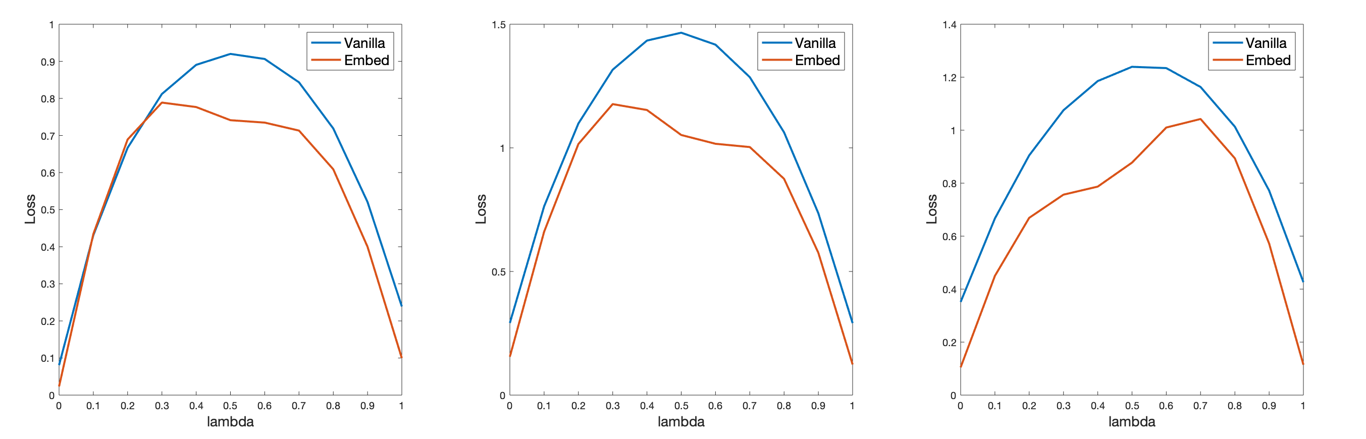
To show that Embed learned better representations in mixup, we next visualized the impact of the two different methods. Figure 3 plots how the loss value of three randomly sampled pairs of test examples changes as a function of in (32). Each subplot here corresponds to a randomly chosen pair. By increasing from 0 to 1 with a step size , we obtained different mixup representations. We then applied the trained classifiers on these representations to compute the loss value. As shown in Figure 3, Embed always has a lower loss, especially when Vanilla is at its peak loss value. Recall in (33), Embed learns representations by considering the that maximizes the change; this figure exactly verified this behavior and Embed learns better representation.
E.2 Additional experiments for structured multilabel prediction
Here, we provide more detailed results for our method applied to structured multilabel prediction, as described in Section 6.
Accuracy on multiple runs.
We repeated the experiment, detailed in Section 7.3 and tabulated in Table 3 ten times for all the three algorithms. Figures 4,5,6 show the accuracy plot of our method (Embed) compared with baselines (ML-SVM and HR-SVM) on Enron (Klimt and Yang 2004), WIPO (Rousu et al. 2006), Reuters (Lewis et al. 2004) datasets with randomly drawn train/test examples over runs.
Comparing constraint violations.
In this experiment, we demonstrate the effectiveness of the model’s ability to embed structures explicitly. Recall that for the structured multilabel prediction task, we wanted to incorporate two types of constraints (i) implication, (ii) exclusion. To test if our model (Embed) indeed learns representations that respect these constraints, we counted the number of test examples that violated the implication and exclusion constraints from the predictions. We repeated the test for ML-SVM and HR-SVM.
We observed that HR-SVM and Embed successfully modeled implications on all the datasets. This is not surprising as HR-SVM takes the class hierarchy into account. The exclusion constraint, on the other hand, is a “derived” constraint and is not directly modeled by HR-SVM. Therefore, on datasets where Embed performed significantly better than HR-SVM, we might expect fewer exclusion violations by Embed compared to HR-SVM. To verify this intuition, we considered the Enron dataset with train/test split where Embed performed better than HR-SVM. The constraint violations are shown as a line plot in Figure 7, with the constraint index on the -axis and number of examples violating the constraint on the -axis.
Recall again that predictions in Embed for multilabel prediction are made using a linear classifier. Therefore the superior performance of Embed in this case, can be attributed to accurate representations learned by the model.



![[Uncaptioned image]](2004.12209v3/images/white.png)