August 11, 2026

Quasi-Normal Modes and Stability of Einstein-Born-Infeld
Black Holes in de Sitter SpacePreprint: arXiv:2004.12185v3 [hep-th]

Chong Oh Lee Note: E-mail address: cohlee@gmail.com Affiliation: Department of Physics, Kunsan National University, Kunsan 54150, Korea Jin Young Kim Note: E-mail address: jykim@kunsan.ac.kr, Corresponding author Affiliation: Department of Physics, Kunsan National University, Kunsan 54150, Korea Mu-In Park Note: E-mail address: muinpark@gmail.com Affiliation: Center for Quantum Spacetime, Sogang University, Seoul, 121-742, Korea

Abstract

We study gravitational perturbations of electrically charged black holes in (3+1)-dimensional Einstein-Born-Infeld gravity with a positive cosmological constant. For the axial perturbations, we obtain a set of decoupled Schrödinger-type equations, whose formal expressions, in terms of metric functions, are the same as those without cosmological constant, corresponding to the Regge-Wheeler equation in the proper limit. We compute the quasi-normal modes (QNMs) of the decoupled perturbations using the Schutz-Iyer-Will’s WKB method. We discuss the stability of the charged black holes by investigating the dependence of quasi-normal frequencies on the parameters of the theory, correcting some errors in the literature. It is found that all the axial perturbations are stable for the cases where the WKB method applies. There are cases where the conventional WKB method does not apply, like the three-turning-points problem, so that a more generalized formalism is necessary for studying their QNMs and stabilities. We find that, for the degenerate horizons with the “point-like” horizons at the origin, the QNMs are quite long-lived, close to the quasi-resonance modes, in addition to the “frozen” QNMs for the Nariai-type horizons and the usual (short-lived) QNMs for the extremal black hole horizons. This is a genuine effect of the branch which does not have the general relativity limit. We also study the exact solution near the (charged) Nariai limit and find good agreements even far beyond the limit for the imaginary frequency parts.

Keywords:

Gravitational Perturbations, Quasi-Normal Modes, Stability of Black Holes, Non-Linear Theories

I Introduction

Recent detections of gravitational waves from the merger of compact astronomical objects confirmed directly the existence of black holes prl116; prl118; prl119. Gravitational waves from the mergers of various compact objects, like black holes or neutron stars, are common in our universe and expected to be observed frequently in the near future. Also the recent observation of the shadow images from a supermassive black hole, along with the observation of gravitational waves, opened a new era to test Einstein’s general relativity (GR) under extreme conditions, like black holes EHTelescope.

The non-linear generalization of Maxwell’s electromagnetism by Born and Infeld (BI) borninfeld1; borninfeld2 was originally developed to obtain a finite self-energy of a point charge by modifying Maxwell’s theory at the short distance. The BI-type action attracted renewed interests as an effective action of D-branes in string theory Leig:1989. When combined with Einstein action, the short distance behaviors of the metric and black hole solutions are different from those of Einstein-Maxwell theory. On the large scale, natural existence of electrically charged black holes is questionable because our universe seems to be charge neutral. However, on the small scale which may be described by Einstein-Born-Infeld (EBI) theory, the charged black holes may exist, as charged elementary particles do at the high energy. It may be also interesting as a preliminary to study the magnetically charged black holes, which may exist from the collapse of neutron stars with a strong magnetic field, known as magnetars magnetar.

Quasi-normal modes (QNMs) are the oscillations with complex frequencies in open systems with energy dissipations. Perturbations of a black hole are described by QNMs and the complex frequencies of QNMs carry the characteristic properties of the black hole like mass, charge, and angular momentum, independent of the initial perturbations. QNMs of black holes have attracted much interest in relation with the gravitational waves since these can be used as a key tool for the test of GR. Theoretically, this also provides a (simple) criterion of the stability, under linear perturbations, of a black hole by looking at the sign of the imaginary part of quasi-normal frequency.

In this paper, we consider electrically charged black holes in EBI gravity with a positive cosmological constant and compute QNMs of gravitational perturbations of EBI black holes. We adopt the Schutz-Iyer-Will’s WKB method Schutz:1985a; iyerwill; iyer for numerical computations of QNMs and consider the axial perturbations for simplicity. We obtain a set of decoupled Schrödinger-type equations, corresponding to Regge-Wheeler equation, whose formal expressions, in terms of metric functions, are the same as those without cosmological constant. We discuss the stability of the charged black holes by investigating the dependence of quasi-normal frequencies on the parameters of the theory, correcting some errors in the literature. It is found that all the axial perturbations are stable for the cases where the WKB method applies. There are cases where the conventional WKB method does not apply, like the three-turning-points problem, so that a more generalized formalism is necessary for studying their QNMs and stabilities. We find that, for the degenerate horizons with the “point-like” horizons at the origin, the QNMs are quite long-lived, close to the quasi-resonance modes (QRMs), in addition to the “frozen” QNMs with the vanishing frequency, ${\omega}\approx 0$ , for the Nariai-type horizons and the usual (short-lived) QNMs for the extremal black hole horizons. This is a genuine effect of the non-GR branch of $\beta Q=1/2$ , which does not have the GR limit $\beta\rightarrow\infty$ with the BI parameter $\beta$ and electric charge $Q$ . We study the exact solution near the (charged) Nariai limit and find good agreements even far beyond the limit for the imaginary frequency parts.

The organization of this paper is as follow. In Sec. 2, we review the electrically charged black hole solution in EBI gravity with a positive cosmological constant. In Sec. 3, we consider the axial perturbations from the spherically symmetric EBI black hole background and obtain a set of decoupled Regge-Wheeler equations. In Sec. 4, we use the Shutz-Iyer-Will’s third-order WKB method to compute the QNMs numerically and discuss the stabilities of the EBI black holes. In Sec. 5, we study the exact solution near the (charged) Nariai limit and compare it with the numerical results in Sec. 4. In Sec. 6, we conclude with several discussions. Throughout this paper, we use the conventional units for the speed of light $c$ , the electric and magnetic constants $\epsilon_{0},\mu_{0}$ , and the Boltzman constant $k_{B}$ , $c=4\mu_{0}=4/\epsilon_{0}=k_{B}=1$ , but keep the Newton constant $G$ and the Planck constant $\hbar$ unless stated otherwise.

II Background Solutions

In this section, we briefly review the black hole solution in EBI gravity with a positive cosmological constant ${\Lambda}$ in $(3+1)$ dimensions, from which the gravitational perturbations will be considered. The EBI action is given by

S=\int d^{4}x\sqrt{-g}\left[\frac{(R-2\Lambda)}{16\pi G}+L(F)\right],

(1)

where the BI Lagrangian density $L(F)$ is given by

L(F)=4\beta^{2}\left(1-\sqrt{1+\frac{F_{\mu\nu}F^{\mu\nu}}{2\beta^{2}}}\right).

(2)

Here, $\beta~$ is the BI’s coupling constant with dimensions $[{\rm length}]^{-2}$ borninfeld1; borninfeld2. In the weak field or equivalently strong coupling limit, $|F_{\mu\nu}F^{\mu\nu}|\ll 2\beta^{2}$ , $L(F)$ may be expanded as

\displaystyle L(F)=-{F}^{2}+\frac{2F^{4}}{\beta^{2}}+{\cal O}\left(\frac{F^{6}}{\beta^{4}}\right),

(3)

where $F^{2}\equiv F_{\mu\nu}F^{\mu\nu}$ and the usual Maxwell’s electrodynamics is recovered at the lowest order. The correction terms, when $F$ is comparable to $\beta$ , represent the effect of the non-linear BI fields at the short distance $\sim\beta^{-1}$ and the possible electromagnetic field strength is bounded by $-F^{2}\leq 2\beta^{2}$ .

Taking $16\pi G=1$ for simplicity, the equations of motion are obtained as

\nabla_{\mu}\left(\frac{F^{\mu\nu}}{\sqrt{1+\frac{F^{2}}{2\beta^{2}}}}\right)=0,

(4)

R_{\mu\nu}-\frac{1}{2}Rg_{\mu\nu}+\Lambda g_{\mu\nu}=\frac{1}{2}T_{\mu\nu},

(5)

where the energy-momentum tensor for BI fields is given by

T_{\mu\nu}=g_{\mu\nu}L(F)+\frac{4F_{\rho\mu}{F^{\rho}}_{\nu}}{\sqrt{1+\frac{F^{2}}{2\beta^{2}}}}.

(6)

Let us now consider a static and spherically symmetric solution with the metric ansatz

ds^{2}=-N^{2}(r)dt^{2}+\frac{1}{f(r)}dr^{2}+r^{2}(d\theta^{2}+\sin^{2}\theta d\phi^{2}).

(7)

For the static, electrically-charged case where the only non-vanishing component of the field strength tensor is $F_{rt}\equiv E_{r}$ , the general solutions for the metric and the BI electric field are obtained as

	$\displaystyle N^{2}(r)$	$\displaystyle=$	$\displaystyle f(r)=1-\frac{2M}{r}-\frac{\Lambda}{3}r^{2}+\frac{2}{3}\beta^{2}r^{2}\left(1-\sqrt{1+\frac{Q^{2}}{\beta^{2}r^{4}}}\right)+\frac{4}{3}\frac{Q^{2}}{r^{2}}~{{}_{2}F}_{1}\left(\frac{1}{2},\frac{1}{4};\frac{5}{4};\frac{-Q^{2}}{\beta^{2}r^{4}}\right),$		(8)
	$\displaystyle E_{r}(r)$	$\displaystyle=$	$\displaystyle\frac{Q}{\sqrt{r^{4}+\frac{Q^{2}}{\beta^{2}}}},$		(9)

in terms of the hypergeometric function Garc:1984; Li:2016. Here $Q$ is the electric charge ¹¹ 1 The charge convention differs from the usual one, like that of Rasheed in Garc:1984. One can convert to the usual convention by replacing $Q\rightarrow Q/16\pi$ . and $M$ is the ADM mass which is composed of the intrinsic mass $C$ and (finite) self energy of a point charge $M_{0}$ , defined by

	$\displaystyle M$	$\displaystyle=$	$\displaystyle C+M_{0},$		(10)
	$\displaystyle M_{0}$	$\displaystyle=$	$\displaystyle\frac{2}{3}\sqrt{\frac{\beta Q^{3}}{\pi}}\Gamma\left(\frac{1}{4}\right)\Gamma\left(\frac{5}{4}\right).$		(11)

In the large-distance limit $r\gg\sqrt{Q/\beta}$ , the solutions become

	$\displaystyle N^{2}$	$\displaystyle=$	$\displaystyle f=1-\frac{\Lambda}{3}r^{2}-\frac{2M}{r}+\frac{Q^{2}}{r^{2}}-\frac{Q^{4}}{20\beta^{2}r^{6}}+{\cal O}(r^{-10}),$		(12)
	$\displaystyle E_{r}$	$\displaystyle=$	$\displaystyle\frac{Q}{r^{2}}-\frac{\beta^{2}Q^{3}}{r^{6}}+{\cal O}(r^{-10}),$		(13)

which show the usual Reissner-Nordstrom-(Anti) de Sitter (RN-(A)dS) black hole at the leading order and the short-distance corrections at the sub-leading orders. On the other hand, in the short-distance limit $r\ll\sqrt{Q/\beta}$ , we have

	$\displaystyle N^{2}$	$\displaystyle=$	$\displaystyle f=1-2\beta Q-\frac{2C}{r}+\frac{1}{3}(2\beta^{2}-\Lambda)r^{2}-\frac{\beta^{3}}{5Q}r^{4}+{\cal O}(r^{6}),$		(14)
	$\displaystyle E_{r}$	$\displaystyle=$	$\displaystyle\frac{Q}{\|Q/\beta\|}-\frac{Q}{2\|Q/\beta\|^{3}}r^{4}+{\cal O}(r^{8}),$		(15)

which show the regularized solutions near the origin, with the milder (curvature) singularity of the metric and the finite electric field at the origin Li:2016; Kim:2016pky due to the non-linear BI fields for a finite coupling $\beta$ .

Refer to caption — Figure 1: The plots of the Hawking temperature $T_{H}$ vs. the (outer) black hole horizon radius $r_{+}$ for varying $\beta Q$ with a fixed $\Lambda>0$ . We consider $\beta Q={2/3,~1/2,~2/4.5,~1/3}$ (bottom to top curves) with $\beta=2$ , $\Lambda=0.2$ .

The solution (8) can have three horizons generally, i.e., two (inner, outer) black hole horizons, $r_{-},r_{+}$ , and one cosmological horizon $r_{++}$ . The Hawking temperature for the outer black horizon $r_{+}$ is given by

	$\displaystyle T_{H}$	$\displaystyle\equiv$	$\displaystyle\frac{\hbar}{4\pi}\left.\frac{df}{dr}\right\|_{r=r_{+}}{}$		(16)
		$\displaystyle=$	$\displaystyle\frac{\hbar}{4\pi}\left[\frac{1}{r_{+}}-{\Lambda}r_{+}+2\beta^{2}r_{+}\left(1-\sqrt{1+\frac{Q^{2}}{\beta^{2}r_{+}^{4}}}\right)\right]$		(16)

and plotted in Fig. 1. There exist two extreme limits of vanishing temperature, when the outer black hole horizon $r_{+}$ meets the inner horizon $r_{-}$ (extremal black holes) or the cosmological horizon $r_{++}$ (Nariai solution), at

\displaystyle r^{*}_{H/C}=\sqrt{\frac{{\Lambda}-2\beta^{2}\pm\sqrt{({\Lambda}-2\beta^{2})^{2}+{\Lambda}({\Lambda}-4\beta^{2})(4\beta^{2}Q^{2}-1)}}{{\Lambda}({\Lambda}-4\beta^{2})}}

(17)

for a positive cosmological constant ${\Lambda}$ ( $r^{*}_{H}<r^{*}_{C}$ ) (Figs. 1 and 2). At the extreme points, the ADM mass $M$ ,

\displaystyle M=\frac{r_{+}}{2}\left[1-\frac{\Lambda}{3}r_{+}^{2}+\frac{2}{3}\beta^{2}r_{+}^{2}\left(1-\sqrt{1+\frac{Q^{2}}{\beta^{2}r_{+}^{4}}}\right)+\frac{4}{3}\frac{Q^{2}}{r_{+}^{2}}~{{}_{2}F}_{1}\left(\frac{1}{2},\frac{1}{4};\frac{5}{4};\frac{-Q^{2}}{\beta^{2}r_{+}^{4}}\right)\right],

(18)

becomes Kim:2016pky; Kim:2018ang

\displaystyle M^{*}=\frac{r^{*}}{3}\left[1+\frac{2Q^{2}}{{r^{*}}^{2}}~{{}_{2}F}_{1}\left(\frac{1}{2},\frac{1}{4};\frac{5}{4};\frac{-Q^{2}}{\beta^{2}{r^{*}}^{4}}\right)\right].

(19)

The first law of black hole thermodynamics is found as

\displaystyle dM=T_{H}dS_{BH}+A_{0}(r_{+})dQ,

(20)

with the usual Bekenstein-Hawking formula for the black hole entropy

\displaystyle S_{BH}=\frac{\pi r_{+}^{2}}{\hbar G},

(21)

and the scalar potential Garc:1984; Cai; Li:2016

\displaystyle A_{0}(r)=\frac{Q}{r}~{{}_{2}F}_{1}\left(\frac{1}{2},\frac{1}{4};\frac{5}{4};\frac{-Q^{2}}{\beta^{2}{r}^{4}}\right).

(22)

The integrated first-law of black hole thermodynamics, called the generalized Smarr relation, is given by Cai; Li:2016; Smar:1972; Liu:2015 ²² 2 The generalized Smarr relation without the last term has been obtained for the planar black holes in Li:2016; Liu:2015. If we consider topological EBI black holes with the topological parameter $k=+1,0,-1$ for spherical, plane, and hyperbolic geometry generally, with the solid angle $\Omega_{k}$ , one finds Cai the last term as $(k/3)\sqrt{4\hbar S_{BH}/{\Omega_{k}G}}$ .

\displaystyle M=\frac{2}{3}\left(S_{BH}T_{H}+QA_{0}(r_{+})\right)+\frac{1}{3}\sqrt{\frac{\hbar S_{BH}}{\pi G}}.

(23)

Now, from the relation (17), one can classify the black holes by the values of $\beta Q$ Kim:2016pky.

(i) $\beta Q>1/2$ : In this case, there are generally three horizons (two smaller ones for black holes and the largest one for the cosmological horizon) for $M_{H}^{*}\leq M\leq M_{C}^{*}~(<M_{0})$ , depending on $M$ and ${\Lambda}$ (Fig. 3, left), where $M_{H}^{*}$ and $M_{C}^{*}$ denote the values of the extremal mass $M^{*}$ in (19) at $r_{H}^{*}$ and $r_{C}^{*}$ for the extremal black holes and the (charged) Nariai solutions, respectively, with the vanishing Hawking temperature (Fig.1). When the mass is outside this range, i.e., $M<M_{H}^{*}$ or $M>M_{C}^{*}$ , the singularity at $r=0$ becomes naked as in the RN black hole.

(ii) $\beta Q=1/2$ : In this case, only the Schwarzschild - de Sitter (Sch-dS) -like black holes with a non-degenerate black hole horizon $r_{+}$ are possible for $M_{0}<M\leq M_{C}^{*}$ (Fig. 3, center). It is peculiar that the black hole horizon $r_{+}$ shrinks to zero size, i.e., the point-like horizon, for the marginal case $M=M_{0}$ (Fig. 4). This corresponds to the extremal black hole, with the vanishing Hawking temperature (Fig.1), where the horizon degenerates at the origin. When the mass $M$ is smaller than the marginal mass $M_{0}$ or larger than $M_{C}^{*}$ , the singularity at $r=0$ becomes naked. Note that, in this case, the GR limit $\beta\rightarrow\infty$ does not exist.

(iii) $\beta Q<1/2$ : This case is similar to the case (ii), except that the marginal case $M=M_{0}$ has no (even a point) horizon so that its curvature singularity at $r=0$ is naked always (Fig. 3, right), even though the (non-degenerate) black hole horizon can arbitrarily approach close to the point-like horizon $r_{+}=0$ in the limit $M\rightarrow M_{0}$ , with the divergent Hawking temperature (Fig. 1) ³³ 3 This behavior of Hawking temperature is similar to that of Sch. black hole. But the difference is that its mass $M$ has still a non-vanishing remnant $M_{0}$ . If this tiny black hole with a unit charge $Q=\sqrt{4\pi\epsilon_{0}\alpha\hbar c}$ ( $\alpha$ is the fine-structure constant) is created at the Planck energy scale in the early universe, i.e., $M_{0}\approx\sqrt{\hbar c/G}$ , we obtain $\beta\approx(9/2)\Gamma(3/4)^{4}\pi^{-7/2}~\alpha^{-3/2}~(\epsilon_{0}\hbar c)^{-1/2}G^{-1}$ . If we consider $\alpha_{Pl}\sim 1.5$ at the early universe, contrast to $\alpha\sim 10^{-2}$ at the current epoch, we have $\beta_{Pl}\sim 0.1~(\epsilon_{0}\hbar c)^{-1/2}G^{-1}$ and $\beta_{Pl}Q\approx 9\Gamma(3/4)^{4}\pi^{-3}~\alpha_{Pl}^{-1}G^{-1}\sim 0.4~G^{-1}$ . .

III Perturbation Equations

In this section, we consider the gravitational perturbations of an electrically charged black hole in EBI gravity with a positive cosmological constant ${\Lambda}>0$ , whose solutions for the metric and fields are given by (8) and (9), respectively. We follow the procedure of Chandrasekhar Chandrasekhar for the perturbations of RN solution but in the different conventions which agree with those of Wald Wald:1984 ⁴⁴ 4 We use a metric with signature $(-+++)$ and the Wald’s conventions for the Riemann and Ricci tensors which differ from Chandrasekhar; Fernando:2004pc; Mell:1989.. We generalize the earlier computations of Fernando:2004pc to a positive cosmological constant but with some important corrections of errors. To accommodate the procedure of Chandrasekhar, it is useful to write the metric (7) as

ds^{2}=-e^{2\nu}dt^{2}+e^{2\psi}d\phi^{2}+e^{2\mu_{2}}dr^{2}+e^{2\mu_{3}}d\theta^{2}

(24)

with

e^{2\nu}\equiv N^{2}(r),~e^{2\mu_{2}}\equiv\frac{1}{f(r)},~e^{2\mu_{3}}\equiv r^{2},~e^{2\psi}\equiv r^{2}\sin^{2}\theta.

(25)

We will consider (24) as a background metric and consider the first-order metric perturbations. In our linear perturbations of the spherically symmetric system, we may restrict ourselves to axisymmetric modes of perturbations, without loss of generality Chandrasekhar, whose metric may be generally written as

ds^{2}=-e^{2\nu}dt^{2}+e^{2\psi}(d\phi-q_{0}dt-q_{2}dr-q_{3}d\theta)^{2}+e^{2\mu_{2}}dr^{2}+e^{2\mu_{3}}d\theta^{2},

(26)

where the metric functions $\nu,\psi,\mu_{2},\mu_{3},q_{0},q_{2}$ , and $q_{3}$ are functions of only $t,r$ , and $\theta$ , due to axisymmetry. There are two kinds of perturbations: The perturbations of $q_{0},q_{2}$ , and $q_{3}$ , which are called “axial” perturbations, induce a dragging effect and impart a rotation to the black hole, whereas the increments of $\delta\nu,\delta\psi,\delta\mu_{2}$ , and $\delta\mu_{3}$ , which are called “polar” perturbations, do not impart such rotation. These two perturbations are decoupled and can be treated independently Chandrasekhar. In this paper, we will focus only on the axial perturbations for simplicity.

To obtain the solutions for the perturbed metric (26), we first need to consider the perturbations of BI and Einstein equations, (4) and (5). For this purpose, we adopt the tetrad formalism as in Chandrasekhar and use the Roman indices $a,b=0,1,2,3$ for the tetrad indices and the Greek indices $\mu,\nu=t,\phi,r,\theta$ for the curved coordinate indices. The tetrad basis $e^{a}_{\mu}$ satisfies $e^{a}_{\mu}e^{b}_{\nu}\eta_{ab}=g_{\mu\nu}$ with $\eta_{ab}={\rm diag}(-1,+1,+1,+1)$ . For the metric given by (26), $e^{a}_{\mu}$ can be obtained as

$\displaystyle e^{0}_{\mu}$	$\displaystyle=$	$\displaystyle(e^{\nu},0,0,0),{}$
$\displaystyle e^{1}_{\mu}$	$\displaystyle=$	$\displaystyle(-q_{0}e^{\psi},e^{\psi},-q_{2}e^{\psi},-q_{3}e^{\psi}),{}$
$\displaystyle e^{2}_{\mu}$	$\displaystyle=$	$\displaystyle(0,0,e^{\mu_{2}},0),{}$
$\displaystyle e^{3}_{\mu}$	$\displaystyle=$	$\displaystyle(0,0,0,e^{\mu_{3}}).$	(27)

Tensors in the two bases are related by the tetrads, for example,

F_{\mu\nu}=e_{\mu}^{a}e_{\nu}^{b}F_{ab},~~R_{\mu\nu}=e_{\mu}^{a}e_{\nu}^{b}R_{ab},

(28)

for the field strength and the Ricci tensor. We will now consider equations of motion (4) and (5) in the tetrad basis.

III.1 The perturbed BI equations

BI fields satisfy the Bianchi identities,

\displaystyle\nabla_{[\mu}F_{\nu\lambda]}=0,

(29)

in addition to the field equations (4). The corresponding two sets of equations for tetrad components of BI fields can be found from the tetrads (27) and the relation (28).

First, from the Bianchi identities (29), one can find four equations as

	$\displaystyle(e^{\psi+\mu_{2}}F_{12})_{,\theta}+(e^{\psi+\mu_{3}}F_{31})_{,r}=0,$		(30)
	$\displaystyle(e^{\psi+\nu}F_{01})_{,r}+(e^{\psi+\mu_{2}}F_{12})_{,t}=0,$		(31)
	$\displaystyle(e^{\psi+\nu}F_{01})_{,\theta}+(e^{\psi+\mu_{3}}F_{13})_{,t}=0,$		(32)
	$\displaystyle(e^{\psi+\mu_{2}}F_{02})_{,\theta}-(e^{\nu+\mu_{3}}F_{03})_{,r}+(e^{\mu_{2}+\mu_{3}}F_{23})_{,t}$
	$\displaystyle=e^{\psi+\nu}F_{01}Q_{23}+e^{\psi+\mu_{2}}F_{12}Q_{03}-e^{\psi+\mu_{3}}F_{13}Q_{02},$		(33)

from the assumed axisymmetry in the tetrads and BI fields. Here, $Q_{ab}$ ’s are defined as

Q_{02}\equiv q_{0,r}-q_{2,t},~~Q_{03}\equiv q_{0,\theta}-q_{3,t},~~Q_{23}\equiv q_{2,\theta}-q_{3,r}.

(34)

Note that (30), (31), and (32) represent the absence of a $U(1)$ magnetic monopole and the Faraday’s law of induction in the curved space. However, (33), which corresponds the $\phi$ -component of the Faraday’s law, shows that there are “induced” source terms on the right hand side which correspond the magnetic currents ${\cal J}_{(m)}\sim\epsilon^{abcd}F_{ab}Q_{cd}$ , due to non-linear interactions between the electromagnetic and gravitational fields.

Second, from BI field equations (4), which may be conveniently written as

\displaystyle\nabla_{\mu}D^{\mu\nu}=0,

(35)

where

D^{\mu\nu}\equiv\frac{F^{\mu\nu}}{\sqrt{1+F^{2}/\beta^{2}}},

(36)

one can find another set of four equations as

	$\displaystyle(e^{\psi+\mu_{3}}D_{02})_{,r}+(e^{\psi+\mu_{2}}D_{03})_{,\theta}=0,$		(37)
	$\displaystyle-(e^{\psi+\nu}D_{23})_{,r}+(e^{\psi+\mu_{2}}D_{03})_{,t}=0,$		(38)
	$\displaystyle(e^{\psi+\nu}D_{23})_{,\theta}+(e^{\psi+\mu_{3}}D_{02})_{,t}=0,$		(39)
	$\displaystyle(e^{\mu_{2}+\mu_{3}}D_{01})_{,t}+(e^{\nu+\mu_{3}}D_{12})_{,r}+(e^{\nu+\mu_{2}}D_{13})_{,\theta}$
	$\displaystyle=e^{\psi+\mu_{3}}D_{02}Q_{02}+e^{\psi+\mu_{2}}D_{03}Q_{03}-e^{\psi+\nu}D_{23}Q_{23}.$		(40)

Here, (37), (38), and (39) represent the Gauss’s law and the Ampere’s law (with the Maxwell’s correction term) in the curved space. On the other hand, (40), which corresponds the $\phi$ -component of the Ampere’s law, shows the induced source terms which correspond the electric currents ${\cal J}_{(e)}\sim F_{ab}Q_{ab}$ , due to non-linear interactions between the electromagnetic and gravitational fields, similar to (33). These induced source terms in (40) and (33) represent the back-reactions from the dynamical metric $q_{0},q_{2}$ and $q_{3}$ , which are also driven by $T_{\mu\nu}$ in the Einstein equations (5).

Up to now, we have not assumed any specific solution of the background BI fields. Now, using that the only non-zero components of $F$ and $D$ in the background solution (9) are

F_{02}=-\frac{Q}{\sqrt{r^{4}+Q^{2}/\beta^{2}}},~~~D_{02}=-\frac{Q}{r^{2}},

(41)

and substituting $\psi,\nu,\mu_{2},\mu_{3}$ with $\psi+\delta\psi,\nu+\delta\nu,\mu_{2}+\delta\mu_{2},\mu_{3}+\delta\mu_{3}$ in the above equations, we find the linearized versions of perturbed BI equations as

$\displaystyle(re^{\nu}F_{01})_{,r}+re^{-\nu}F_{12,t}$	$\displaystyle=$	$\displaystyle 0,$	(42)
$\displaystyle re^{\nu}(F_{01}\sin\theta)_{,\theta}+r^{2}F_{13,t}\sin\theta$	$\displaystyle=$	$\displaystyle 0,$	(43)
$\displaystyle re^{-\nu}D_{01,t}+(re^{\nu}D_{12})_{,r}+D_{13,\theta}$	$\displaystyle=$	$\displaystyle-Q(q_{0,2}-q_{2,0})\sin\theta,$	(44)

$\displaystyle-(re^{\nu}D_{23})_{,r}+re^{-\nu}D_{03,t}$	$\displaystyle=$	$\displaystyle 0,$	(45)
$\displaystyle\delta D_{02,t}-\frac{Q}{r^{2}}(\delta\psi+\delta\mu_{3})_{,t}+\frac{e^{\nu}}{r\sin\theta}(D_{23}\sin\theta)_{,\theta}$	$\displaystyle=$	$\displaystyle 0,$	(46)
$\displaystyle\left[\delta F_{02}-\frac{Q}{\sqrt{r^{4}+Q^{2}/\beta^{2}}}(\delta\nu+\delta\mu_{2})\right]_{,\theta}+(re^{\nu}F_{30})_{,r}+re^{-\nu}F_{23,t}$	$\displaystyle=$	$\displaystyle 0.$	(47)

III.2 The perturbed Ricci tensor equations

To find the metric perturbations of the Einstein equation (5), we may conveniently write the Einstein equations (5) as ⁵⁵ 5 The energy-momentum part in the right-hand side of (48) coincides with $``T_{\mu\nu}"$ for Maxwell’s electro magnetism. But, in BI theory, it is not valid generally. This is one of the errors in Fernando:2004pc which may affect the polar perturbations in EBI gravity.

	$\displaystyle R_{\mu\nu}$	$\displaystyle=$	$\displaystyle\frac{1}{2}\left(T_{\mu\nu}-\frac{1}{2}g_{\mu\nu}{T^{\gamma}}_{{\gamma}}\right)+{\Lambda}g_{\mu\nu}$		(48)
		$\displaystyle=$	$\displaystyle\frac{2}{\sqrt{1+\frac{F^{2}}{2\beta^{2}}}}\left[g^{{\gamma}{\delta}}F_{\mu{\gamma}}F_{\nu{\delta}}+g_{\mu\nu}~\beta^{2}\left(1-\sqrt{1+\frac{F^{2}}{2\beta^{2}}}\right)\right]+{\Lambda}g_{\mu\nu}$		(49)

\displaystyle R_{ab}=\frac{2}{\sqrt{1+\frac{F^{2}}{2\beta^{2}}}}\left[\eta^{cd}F_{ac}F_{bd}+\eta_{ab}~\beta^{2}\left(1-\sqrt{1+\frac{F^{2}}{2\beta^{2}}}\right)\right]+{\Lambda}\eta_{ab}

(50)

in the tetrad basis, where $F^{2}\equiv F_{\mu\nu}F^{\mu\nu}=F_{ab}F^{ab}$ .

With a simple computation, one can easily find that the cosmological constant term does not appear explicitly in the perturbation of Einstein equations (48). The lineralized form of the perturbed Ricci tensor equations are then given by

\displaystyle\delta R_{ab}=\frac{2}{\sqrt{1+\frac{F^{2}}{2\beta^{2}}}}\left[-\frac{1}{2}F_{cd}\delta F_{cd}\left(\frac{\eta_{ab}+\eta^{cd}F_{ac}F_{bd}/\beta^{2}}{1+\frac{F^{2}}{2\beta^{2}}}\right)+\eta^{cd}\left(\delta F_{ac}F_{bd}+F_{ac}\delta F_{bd}\right)\right].

(51)

Since the only non-zero componsnt of the background $F_{ab}$ is $F_{02}$ , we replace $\delta F_{ab}$ by $F_{ab}$ except for $\delta F_{02}$ for simplification, following Chandrasekhar. Explicit forms of the right-hand side of the perturbed Ricci tensors (51) are given by

$\displaystyle\delta R_{00}$	$\displaystyle=-\delta R_{22}=-\frac{2Q}{r^{2}}\delta F_{02},$	(52)
$\displaystyle\delta R_{11}$	$\displaystyle=\delta R_{33}=-\frac{2Q}{r^{2}}\left(1+\frac{Q^{2}}{\beta^{2}r^{4}}\right)\delta F_{02},$	(53)
$\displaystyle\delta R_{01}$	$\displaystyle=-\frac{2Q}{r^{2}}F_{12},$	(54)
$\displaystyle\delta R_{02}$	$\displaystyle=0,$	(55)
$\displaystyle\delta R_{03}$	$\displaystyle=\frac{2Q}{r^{2}}F_{23},$	(56)
$\displaystyle\delta R_{12}$	$\displaystyle=\frac{2Q}{r^{2}}F_{01},$	(57)
$\displaystyle\delta R_{13}$	$\displaystyle=0,$	(58)
$\displaystyle\delta R_{23}$	$\displaystyle=\frac{2Q}{r^{2}}F_{03}.$	(59)

III.3 The wave equations for the axial perturbations

The linearized Einstein equations can be obtained by equating $\delta R_{ab}$ of the left-hand side in the above equations with those which can be computed from the Ricci tensors for the metric (26) in the tetrad basis, whose explicit forms are given in the Appendix. As mentioned before, the perturbation equations can be categorized into two kinds. One is the axial perturbations which are characterized by the non-vanishing of $q_{0},q_{2},q_{3},F_{01},F_{12}$ , and $F_{13}$ . The other is the polar perturbations which are characterized by the non-vanishing of $\delta F_{02},F_{03},F_{23},\delta\nu,\delta\psi,\delta\mu_{2}$ , and $\delta\mu_{3}$ . In this paper, we only consider the axial perturbations, which are relatively easier and can be treated independently of the polar perturbations. For this purpose, we first consider (57) and (58), which are now given by

	$\displaystyle(r^{2}e^{2\nu}Q_{23}\sin^{3}\theta)_{,\theta}+r^{4}Q_{02,t}\sin^{3}\theta$	$\displaystyle=$	$\displaystyle 4Qre^{\nu}F_{01}\sin^{2}\theta,$		(60)
	$\displaystyle(r^{2}e^{2\nu}Q_{23}\sin^{3}\theta)_{,r}-r^{2}e^{-2\nu}Q_{03,t}\sin^{3}\theta$	$\displaystyle=$	$\displaystyle 0~.$		(61)

Eliminating $D_{12}$ and $D_{13}$ from (44) using (42) and (43), we obtain

\left[\frac{e^{2\nu}}{\gamma}(re^{\nu}\gamma\widetilde{\cal D})_{,r}\right]_{,r}+\frac{e^{\nu}}{r}\left(\frac{\widetilde{\cal D}_{,\theta}}{\sin\theta}\right)_{,\theta}\sin\theta-re^{-\nu}\widetilde{\cal D}_{,t,t}=Q(q_{0,2}-q_{2,0})_{,t}\sin^{2}\theta,

(62)

where

{\cal F}\equiv F_{01}\sin\theta,~~\widetilde{\cal D}\equiv D_{01}\sin\theta=\frac{{\cal F}}{\gamma},

(63)

with

\gamma\equiv\sqrt{1-\frac{F_{02}^{2}}{\beta^{2}}}=\frac{1}{\sqrt{1+\frac{Q^{2}}{\beta^{2}r^{4}}}}~.

(64)

With the substitution

{\widetilde{Q}}(r,\theta,t)\equiv r^{2}e^{2\nu}Q_{23}\sin^{3}\theta=\Delta(q_{2,3}-q_{3,2})\sin^{3}\theta,

(65)

(60) and (61) take the forms

	$\displaystyle\frac{1}{r^{4}\sin^{3}\theta}\frac{\partial{\tilde{Q}}}{\partial\theta}$	$\displaystyle=$	$\displaystyle-(q_{0,2}-q_{2,0})_{,t}+\frac{4Q}{r^{3}\sin^{2}\theta}~e^{\nu}\gamma\widetilde{\cal D},$		(66)
	$\displaystyle\frac{\Delta}{r^{4}\sin^{3}\theta}\frac{\partial{\tilde{Q}}}{\partial r}$	$\displaystyle=$	$\displaystyle(q_{0,3}-q_{3,0})_{,t}~,$		(67)

where $\Delta\equiv r^{2}e^{2\nu}$ . Assuming that the perturbed fields $q_{0},q_{2},q_{3}$ , and ${\widetilde{Q}}$ have a time dependence $e^{-i\omega t}$ and eliminating $q_{0}$ from (66) and (67), we obtain

r^{4}\left(\frac{\Delta}{r^{4}}\frac{\partial{\tilde{Q}}}{\partial r}\right)_{,r}+\sin^{3}\theta\left(\frac{1}{\sin^{3}\theta}\frac{\partial{\tilde{Q}}}{\partial\theta}\right)_{,\theta}+\omega^{2}\frac{r^{4}}{\Delta}\tilde{Q}=4Qe^{\nu}r\left(\frac{\gamma\widetilde{\cal D}}{\sin^{2}\theta}\right)_{,\theta}\sin^{3}\theta~.

(68)

Similarly, eliminating $(q_{0,2}-q_{2,0})_{,t}$ from (62) using (66), we obtain

\left[\frac{e^{2\nu}}{\gamma}(re^{\nu}\gamma\widetilde{\cal D})_{,r}\right]_{,r}+\frac{e^{\nu}}{r}\left(\frac{\widetilde{\cal D}_{,\theta}}{\sin\theta}\right)_{,\theta}\sin\theta+\left(\omega^{2}re^{-\nu}-\frac{4Q^{2}e^{\nu}\gamma}{r^{3}}\right)\widetilde{\cal D}=-Q\frac{{\widetilde{Q}}_{,\theta}}{r^{4}\sin\theta}~.

(69)

We can further separate the variables $r$ and $\theta$ in (68) and (69) with

{\tilde{Q}}(r,\theta)={\cal Q}(r)C^{-3/2}_{l+2}(\theta),

(70)

and

\widetilde{\cal D}(r,\theta)=\frac{{\cal D}(r)}{\sin\theta}\frac{dC^{-3/2}_{l+2}}{d\theta}=3{\cal D}(r)C^{-1/2}_{l+1}(\theta),

(71)

where $C_{n}^{m}$ is the Gegenbauer function and we have used the recurrence relation,

\frac{1}{\sin\theta}\frac{dC_{n}^{m}}{d\theta}=-2mC_{n-1}^{m+1}~.

(72)

Substituting (70) and (71) in (68) and (69), we obtain two radial wave equations,

\Delta\frac{d}{dr}\left(\frac{\Delta}{r^{4}}\frac{d{\cal Q}}{dr}\right)-\mu^{2}\frac{\Delta}{r^{4}}{\cal Q}+\omega^{2}{\cal Q}=-\frac{4Q}{r^{3}}\mu^{2}\Delta e^{\nu}\gamma{\cal D},

(73)

\left[\frac{e^{2\nu}}{\gamma}(re^{\nu}\gamma{\cal D})_{,r}\right]_{,r}-(\mu^{2}+2)\frac{e^{\nu}}{r}{\cal D}+\left(\omega^{2}re^{-\nu}-\frac{4Q^{2}e^{\nu}\gamma}{r^{3}}\right){\cal D}=-Q\frac{{\cal Q}}{r^{4}},

(74)

where

\mu^{2}\equiv(l-1)(l+2)

(75)

and $l=0,1,2,\cdots$ denotes the orbital number.

Introducing the tortoise coordinate $r_{*}$ ,

\frac{d}{dr_{*}}=e^{2\nu}\frac{d}{dr}

(76)

and further defining ${\cal Q}$ and ${\cal D}$ as

{\cal Q}\equiv rH_{2},~~~re^{\nu}\gamma{\cal D}\equiv-\frac{H_{1}e^{-\frac{\varphi}{2}}}{2\mu}

(77)

with

e^{\varphi}\equiv\frac{1}{\gamma}=\sqrt{1+\frac{Q^{2}}{\beta^{2}r^{4}}},

(78)

we find a pair of coupled equations of $H_{1}$ and $H_{2}$ Fernando:2004pc as

	$\displaystyle\widetilde{\bf V}H_{2}$		$\displaystyle=\frac{\Delta}{r^{5}}\left\{\left[\mu^{2}r-(e^{2\nu}r)^{\prime}r+3e^{2\nu}r\right]H_{2}+2\mu Qe^{-\frac{\varphi}{2}}H_{1}\right\},$		(79)
	$\displaystyle\widetilde{\bf V}H_{1}$		$\displaystyle=\frac{\Delta}{r^{5}}\left\{\left[(\mu^{2}+2)r+\frac{4Q^{2}e^{-\varphi}}{r}+r^{3}\left(\frac{(\varphi^{\prime}e^{2\nu})^{\prime}}{2}+\frac{(\varphi^{\prime})^{2}e^{2\nu}}{4}\right)\right]H_{1}+2\mu Qe^{-\frac{\varphi}{2}}H_{2}\right\},$		(80)

where

\widetilde{\bf V}\equiv\frac{d^{2}}{dr_{*}^{2}}+\omega^{2}~.

(81)

To find the one-dimensional Schrödinger-type wave equations, we rewrite the coupled equations (79) and (80) in the matrix form,

\widetilde{\bf V}\pmatrix{H_{1}\cr H_{2}}=\frac{\Delta}{r^{5}}\pmatrix{V_{11}&V_{12}\cr V_{21}&V_{22}}\pmatrix{H_{1}\cr H_{2}},

(82)

where

$\displaystyle V_{11}$	$\displaystyle\equiv V_{1}=(\mu^{2}+2)r+\frac{4Q^{2}e^{-\varphi}}{r}+r^{3}\left(\frac{(\varphi^{\prime}e^{2\nu})^{\prime}}{2}+\frac{(\varphi^{\prime})^{2}e^{2\nu}}{4}\right),$	(83)
$\displaystyle V_{12}$	$\displaystyle=V_{21}=2\mu Qe^{-\frac{\varphi}{2}},$	(84)
$\displaystyle V_{22}$	$\displaystyle\equiv V_{2}=\mu^{2}r-(e^{2\nu}r)^{\prime}r+3e^{2\nu}r.$	(85)

The matrix $V_{ij}$ can be diagonalized by the similarity transformation as in the RN case Chandrasekhar. Then, the two decoupled, one-dimensional Schrödinger-type equations are given by,

\widetilde{\bf V}Z_{i}=U_{i}Z_{i},~~~(i=1,2),

(86)

where the effective potentials, $U_{1}$ and $U_{2}$ , which are real-valued functions, are given by

	$\displaystyle U_{1}$		$\displaystyle=\frac{\Delta}{r^{5}}\left[\frac{V_{1}+V_{2}}{2}+\sqrt{\left(\frac{V_{1}-V_{2}}{2}\right)^{2}+V_{12}^{2}}\right],$		(87)
	$\displaystyle U_{2}$		$\displaystyle=\frac{\Delta}{r^{5}}\left[\frac{V_{1}+V_{2}}{2}-\sqrt{\left(\frac{V_{1}-V_{2}}{2}\right)^{2}+V_{12}^{2}}\right].$		(88)

Here, the decoupled solutions $Z_{1}$ and $Z_{2}$ are related with the coupled solutions $H_{1}$ and $H_{2}$ , which are basically the perturbations of the metric variable $Q_{23}$ and the fields strength $D_{01}$ Chandrasekhar,

\displaystyle\pmatrix{Z_{1}\cr Z_{2}}=\frac{1}{\sqrt{q_{1}(q_{1}-q_{2})}}\pmatrix{q_{1}H_{1}+\sqrt{-q_{1}q_{2}}H_{2}\cr-\sqrt{-q_{1}q_{2}}H_{1}+q_{1}H_{2}},

(89)

where

	$\displaystyle q_{1}$		$\displaystyle=\frac{V_{1}-V_{2}}{2}+\sqrt{\left(\frac{V_{1}-V_{2}}{2}\right)^{2}+V_{12}^{2}},$		(90)
	$\displaystyle q_{2}$		$\displaystyle=\frac{V_{1}-V_{2}}{2}-\sqrt{\left(\frac{V_{1}-V_{2}}{2}\right)^{2}+V_{12}^{2}}.$		(91)

The explicit form of $U_{1},U_{2},q_{1},$ and $q_{2}$ will be available upon substituting $e^{2\nu}$ and $e^{\varphi}$ with the background solutions (25) and (78), respectively, when we compute the QNMs in the next section.

IV Quasi-Normal Modes for the Axial Perturbations: The WKB approach

IV.1 The WKB approximation

Quasi-Normal Modes (QNMs) are defined as the solutions which are purely ingoing as $e^{-i(\omega t+kr_{*})}$ near the (outer) black hole horizon $r_{+}$ , where $r_{*}=-\infty$ . In this paper, in order to compute QNMs, we will consider the WKB approximation method Schutz:1985a; iyerwill; iyer, which is simple to apply in our case though there are several inherent limitations, as will be explained below. The applicability depends also on several conditions, like the (asymptotic) boundary conditions, and our dS space-time satisfies this condition which is a technical reason of using the WKB approach in this paper. In this section, we briefly summarize the basic results of the WKB approach.

The master equation for the WKB approach may be written as the one-dimensional Schödinger-type equation ⁶⁶ 6 In contrast to the usual Schödinger equation in quantum mechanics, the potential ${\bf Q}$ can be complex-valued generally.,

\displaystyle\frac{d^{2}}{dx^{2}}\Phi(x)+{\bf Q}(x)\Phi(x)=0,

(92)

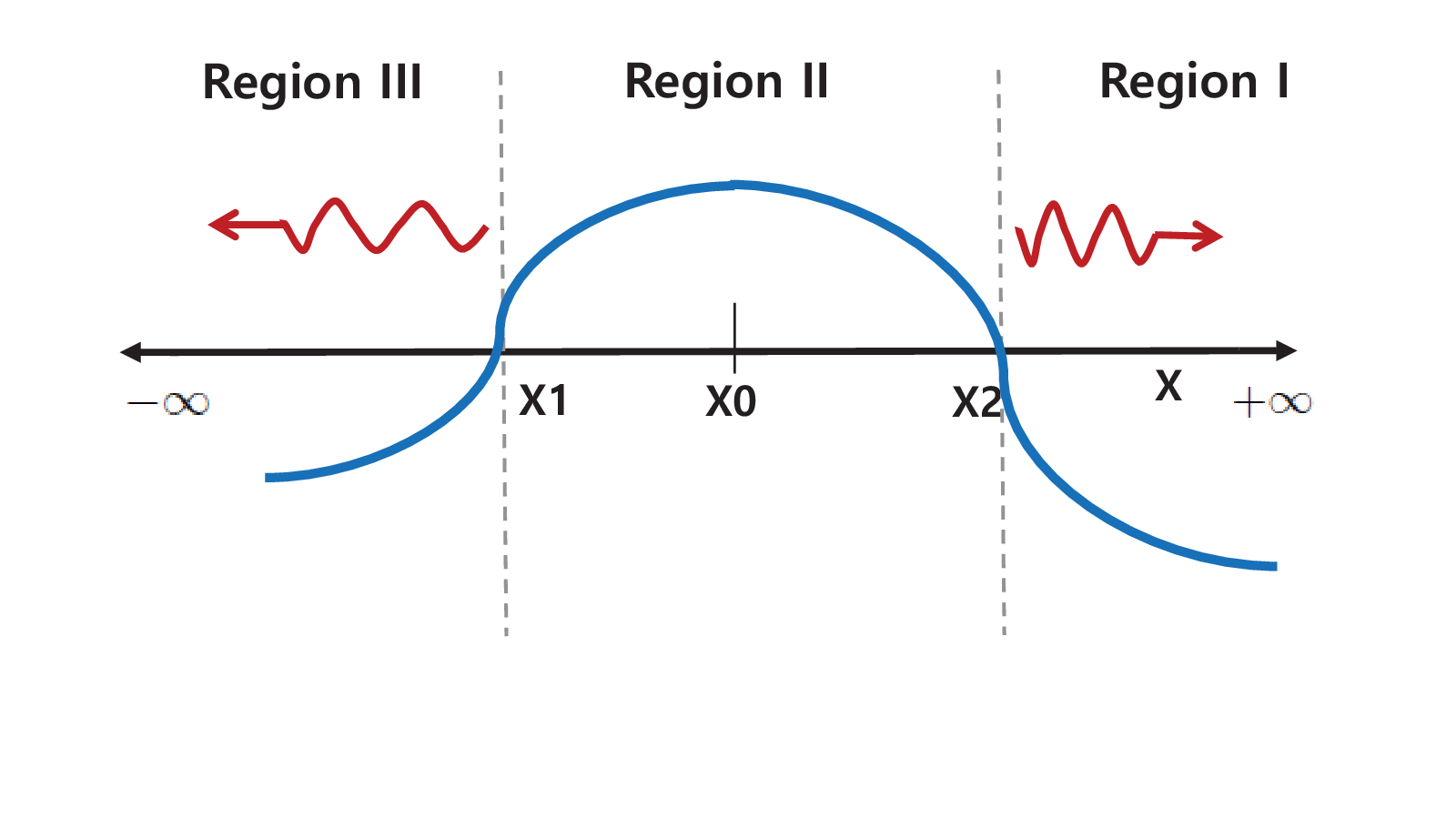
where the potential function $-{\bf Q}(x)$ is assumed to be constant at the asymptotic boundaries $x=\pm\infty$ , although not necessary the same at both ends, and has one maximum at a certain finite $x_{0}$ (Fig. 5). In the black hole case, $\Phi$ represents the radial part of the perturbation with the usual time dependence of a positive-frequency mode $e^{-i\omega t}$ , as well as the appropriate angular dependence. The coordinate $x$ is related to the tortoise coordinate $r_{*}$ which ranges from $-\infty$ , at the (outer) black hole horizon $r_{+}$ , to $+\infty$ , at the spatial infinity $r=\infty$ for the asymptotically flat iyerwill or at the cosmological horizon $r_{++}$ for the asymptotically dS case Mell:1989, as adopted in this paper.

In order to solve the one-dimensional potential barrier problem of (92), we adopt a modified WKB approach by matching the two exterior WKB solutions in regions I and III across the two turning points $x_{1}$ and $x_{2}$ simultaneously Bend. In the interior region II, we expand the potential function $-{\bf Q}(x)$ near its maximum at $x=x_{0}$ and use it to connect the two exterior WKB solutions. For the black hole case with the quasi-normal mode boundary conditions, i.e., purely “outgoing” (from the potential barrier), the result may be written as the simple semi-analytic formula,

\displaystyle\frac{i{\bf Q}_{0}}{\sqrt{2{\bf Q}_{0}^{\prime\prime}}}-i\sum^{N}_{k=1}\widetilde{\Lambda}_{2k}-\sum^{\widetilde{N}}_{k=1}\Omega_{2k+1}=n+\frac{1}{2},

(93)

where the primes denote the derivatives in terms of $x$ and ${\bf Q}_{0}^{\prime\prime}>0$ due to the extremum of the potential $-{\bf Q}$ at $x_{0}$ . Here, the subscripts $2k,2k+1$ denote the order of the WKB approximations, $\widetilde{N}=N$ or $N\pm 1$ , and $\widetilde{\Lambda}_{2k}$ , $\Omega_{2k+1}$ are polynomials of the derivatives ${\bf Q}_{0}^{(m)}/{\bf Q}_{0}^{\prime\prime}$ and $\sqrt{{\bf Q}_{0}^{\prime\prime}}$ . It is important to note that even and odd-order terms become pure-imaginary and real-valued, respectively, so that, when considering ${\bf Q}_{0}={\omega}^{2}-U_{0}$ in the black hole case, they play the distinct roles in obtaining the quasi-normal frequencies, ${\omega}={\omega}_{R}-i{\omega}_{I}$ ⁷⁷ 7 This fact does not seem to be well emphasized in the literature. This causes some misleading results, for example, in Fernando:2004pc due to the related typos in the original work of the third-order terms in iyerwill where $``i"$ factor in the even part of (93) is missing. Similar typos also appear in the 4th-order terms in Konoplya:2003ii (Appendix A), in contrast to the correct $i$ factors in the corresponding 4th-order terms in iyerwill (Appendix) and Matyjasek:2017psv (private communications: We thank the authors for kindly sharing their results)..

Then, the result up to the third WKB orders iyerwill; iyer ⁸⁸ 8 The convergence in each order may not be guaranteed generally since the expansions are just asymptotic ones. However, the popular third-order result of iyerwill can also be obtained as the lower-order results of the phase integral approach which allows the convergent expansions with controlled accuracy Galt:1991 and works well in many cases. For extensions to higher orders, see iyerwill (Appendix) (4th order), Konoplya:2003ii (6th order), and Matyjasek:2017psv (13th order). See also Kono:2019 for a recent review., with ${\bf Q}\equiv{\omega}^{2}-U$ from (86), is given by

\omega^{2}=\left[U_{0}+\sqrt{-2U_{0}^{\prime\prime}}~\widetilde{\Lambda}_{2}\right]-i\left(n+\frac{1}{2}\right)\sqrt{-2U_{0}^{\prime\prime}}~\left(1+\widetilde{\Omega}_{3}\right)

(94)

with the real-valued WKB correction terms,

$\displaystyle\widetilde{\Lambda}_{2}$	$\displaystyle=$	$\displaystyle\frac{1}{\sqrt{-2U_{0}^{\prime\prime}}}\left[\frac{1}{32}\left(\frac{U_{0}^{(4)}}{U_{0}^{\prime\prime}}\right)\left(1+4\alpha^{2}\right)-\frac{1}{288}\left(\frac{U_{0}^{(3)}}{U_{0}^{\prime\prime}}\right)^{2}(7+60\alpha^{2})\right],$	(95)
$\displaystyle\widetilde{\Omega}_{3}$	$\displaystyle=$	$\displaystyle\frac{1}{-2U_{0}^{\prime\prime}}\left[\frac{5}{6912}\left(\frac{U_{0}^{(3)}}{U_{0}^{\prime\prime}}\right)^{4}(77+188\alpha^{2})-\frac{1}{384}\left(\frac{{U_{0}^{(3)}}^{2}U_{0}^{(4)}}{{U_{0}^{\prime\prime}}^{3}}\right)(51+100\alpha^{2})\right.$	(96)
		$\displaystyle+\left.\frac{1}{2304}\left(\frac{U_{0}^{(4)}}{U_{0}^{\prime\prime}}\right)^{2}(67+68\alpha^{2})+\frac{1}{288}\left(\frac{U_{0}^{(3)}U_{0}^{(5)}}{{U_{0}^{\prime\prime}}^{2}}\right)(19+28\alpha^{2})-\frac{1}{288}\left(\frac{U_{0}^{(6)}}{U_{0}^{\prime\prime}}\right)(5+4\alpha^{2})\right],$	(96)

where $\alpha\equiv n+\frac{1}{2}~(n=0,1,2,\cdots),$ $\widetilde{\Omega}_{3}\equiv{\Omega}_{3}/(n+1/2)$ , and the primes and the superscript $(m)$ of $U^{(m)}_{0}$ denote the derivatives of the effective potential $U(r_{\ast})$ with respect to the tortoise coordinate $r_{\ast}$ , evaluated at its maximum point $r_{0}$ . The maximum point $r_{0}$ is determined by ${dU}/{dr_{*}}=e^{2\nu}{dU}/{dr}=0,$ which does not have analytic solutions in our case, where the effective potentials $U_{i}$ in (87) and (88) are quite complicated so that $r_{0}$ can be found only numerically. Then, QNMs can be found numerically by solving (94) from the numerical computations of (95) and (96) as a function of the parameters of the theory.

IV.2 QNMs vs. $\beta$

Figs. 6 and 7 show the effective potentials and corresponding lowest (i.e., fundamental) QNMs with $n=0$ as functions of the BI parameter $\beta$ . As can be seen in Fig. 6 (left), there are one degenerate event horizon for $\beta=\beta_{\rm min}$ , and one degenerate black hole horizon with one cosmological horizon for $\beta=\beta_{\rm max}$ . In between them, $\beta_{\rm min}<\beta<\beta_{\rm max}$ , there are generally three horizons (two black hole horizons and one cosmological horizon), depending on $\beta$ . Only for this dS black hole regime, the WKB formula (94) for QNMs may apply. Fig. 7 shows that the black holes are stable for the range of $\beta_{\rm min}<\beta\leq\beta_{\rm max}$ since their metric perturbations are decaying (which is called also as the“ring-down” phase) with the decay time $\tau\sim{\omega}_{I}^{-1}$ for ${\omega}_{I}>0$ . Moreover, the results show ${\omega}\approx 0$ ⁹⁹ 9 Hereafter, when we denote ${\omega}\approx 0$ , it means zero with the accuracy of $10^{-9}\sim 10^{-8}$ ., i.e., the “frozen” mode, at $\beta=\beta_{\rm min}\approx 0.103$ and no QNMs beyond $\beta_{\rm max}\approx 1.166$ , where the WKB formula (94) does not apply, as expected from the behaviors of the metric functions and the effective potentials in Fig. 6. As $\beta$ increases, the negative imaginary parts of QNMs, ${\omega}_{I}$ increase first monotonically and reach maximum points around $\beta Q=1/2$ (here, $\beta=0.5$ with $Q=1$ ), which divides the Sch-type and the RN-type Kim:2016pky, and then decrease monotonically. Beyond the above range, $\beta<\beta_{\rm min}$ or $\beta>\beta_{\rm max}$ , one can not say anything about its stability since the WKB formula for QNMs can not apply due to the lack of the required boundary conditions and we need other analysis to test its stability. For example, the WKB formula does not say anything about the stability of the naked singularity for $\beta>\beta_{\rm max}$ . On the other hand, the real parts of QNMs ${\omega}_{R}$ increase monotonically and saturate to maximum values, corresponding to those of the RN-dS case Kokk:1988; Mell:1989, showing two decoupled oscillation modes with a rough relation, ${\omega}_{R(1)}\sim 2{\omega}_{R(2)}$ . This is in contrast to the imaginary parts with a rough relation, ${\omega}_{I(1)}\sim{\omega}_{I(2)}$ , so that the real-to-imaginary frequency ratios are ${\omega}_{R(1)}/{\omega}_{I(1)}\sim 2{\omega}_{R(2)}/{\omega}_{I(2)}\sim 10$ .

IV.3 QNMs vs. $Q$

Figs. 8 and 9 show the effective potentials and corresponding lowest QNMs as functions of the electric charge $Q$ . As can be seen in Fig. 8, there are one degenerate event horizon (charged Nariai solution) with one Cauchy horizon for $Q=Q_{\rm min}$ , and one degenerate black hole horizon with one cosmological horizon for $Q=Q_{\rm max}$ . In between them, $Q_{\rm min}<Q<Q_{\rm max}$ , there are generally three (two black hole and one cosmological) horizons, depending on $Q$ . The results show ${\omega}\approx 0$ at $Q=Q_{\rm min}\approx 0.9320$ and no QNMs beyond $Q_{\rm max}\approx 1.0041$ , as expected from the behaviors of the metric functions and the effective potentials in Fig. 8. The behaviors of ${\omega}_{I}$ and ${\omega}_{R}$ are almost the same as those of Fig. 7 for $\beta<0.5$ with the similar relations, ${\omega}_{R(1)}\sim 2{\omega}_{R(2)}$ , ${\omega}_{I(1)}\sim{\omega}_{I(2)}$ and ${\omega}_{R(1)}/{\omega}_{I(1)}\sim 2{\omega}_{R(2)}/{\omega}_{I(2)}\sim 10$ , and other discussions are similar.

IV.4 QNMs vs. $M$

Here, we divide into three cases depending on the values of $\beta Q$ , which divides Sch-type and RN-type by $\beta Q=1/2$ Kim:2016pky. First of all, Figs. 10 and 11 show the effective potentials and corresponding lowest QNMs as functions of the mass $M$ for a RN-type black hole with fixed $\beta Q>1/2$ . As can be seen in Fig. 10, there are one degenerate event horizon (chraged Nariai solution) with one Cauchy horizon for $M=M_{\rm max}$ , and one degenerate black hole horizon with one cosmological horizon for $M=M_{\rm min}$ . In between them, $M_{\rm min}<M<M_{\rm max}$ , there are generally three horizons, depending on $M$ . Fig. 11 shows that ${\omega}\approx 0$ at $M=M_{\rm max}\approx 0.9836$ and no QNMs below $M_{\rm min}\approx 0.9464$ , corresponding to replacing $Q_{\rm min}\rightarrow M_{\rm max}$ and $Q_{\rm max}\rightarrow M_{\rm min}$ in Fig. 9.

Figs. 12 and 13 show the cases for $\beta Q=1/2$ . The basic difference from the case of $\beta Q>1/2$ in Figs. 10 and 11 is that there is only one degenerate (black hole) horizon at the origin $r=0$ , i.e., the point-like horizon, with the vanishing Hawking temperature $T_{H}=0$ and ${\omega}_{I}\approx 1.844\times 10^{-4}$ (for $U_{1}$ ), $1.840\times 10^{-4}$ (for $U_{2}$ ) at $M=M_{\rm min}=M_{0}\approx 0.8740$ . On the other hand, ${\omega}_{I}\approx 0$ at $M=M_{\rm max}\approx 0.9810$ and $\omega_{I}$ has a maximum point about $M\sim 0.9$ . However, the behavior of ${\omega}_{R}$ is similar to the case of $\beta Q>1/2$ in Fig. 10, except the rapid but finite oscillation near $M_{\rm min}$ .

Figs. 14 and 15 show the cases for a Sch-type black hole with $\beta Q<1/2$ . The basic difference from the case of $\beta Q=1/2$ in Figs. 12 and 13 is that there is no (even a point) black hole horizon in addition to the cosmological horizon for $M=M_{\rm min}$ , even though the (non-degenerate) black hole horizon can arbitrarily approach close to $r_{+}=0$ as $M\rightarrow M_{0}$ , with the divergent Hawking temperature (Fig. 1). One more remarkable difference is that, as $M\rightarrow M_{\rm min}$ , $\omega$ is divergent as

\displaystyle\omega_{I}\approx(M-M_{\rm{min}})^{-a}e^{-b},~~\omega_{R}\approx(M-M_{\rm{min}})^{-c}e^{-d}

(97)

with $(a,~b,~c,~d)\approx(1.1223,~5.2870,~1.0752,~2.5693),~(1.1241,~5.3062,~1.0950,~3.2682)$ for $U_{1}$ , $U_{2}$ , respectively, within the limited results due to numerical errors ¹⁰¹⁰ 10 In the numerical computations of WKB formula (93), we find that the “smallness” of $U_{0}^{\prime}$ , which should be “0” by definition, can be a good barometer of the numerical errors. As $M\rightarrow M_{\rm min}$ , the (non-vanishing) magnitude of $U_{0}^{\prime}$ is increasing as shown in Fig. 17. . There is one degenerate horizon where the black hole horizon meets the cosmological horizon for $M=M_{\rm max}$ and generally two (one for black hole and one for cosmological) horizons in between them, $M_{\rm min}<M<M_{\rm max}$ . However, Fig. 15 shows ${\omega}\approx 0$ at $M_{\rm max}\approx 0.9774$ , similarly to the case of $\beta Q>1/2$ in Fig. 11.

IV.5 QNMs vs. $l$

We also divide into three cases depending on the values of $\beta Q$ . Figs. 18 and 19 show the effective potentials and corresponding lowest QNMs as functions of the orbital number $l$ for a fixed $\beta Q>1/2$ . As shown in Fig. 18, there are three (two for black hole and one for cosmological) horizons independent of $l$ (Fig. 18 (left)). On the other hand, the effective potentials depend on $l$ , representing the angular momentum barriers for higher $l$ with a single maximum. However, for lower $l$ , there is no local maximum (but a minimum) in the effective potential ( $l=0$ case for $U_{2}$ ) or there are “three turning points” with one additional turning point within the usual two turning points, i.e., the outer black hole horizon at $r_{+}\approx 1.2$ and the cosmological horizon at $r_{++}\approx 2.4$ ( $l=0$ case for $U_{1}$ and $l=1$ case for $U_{2}$ ) so that the usual WKB formula does not apply ¹¹¹¹ 11 For three-turning-point problems, a complex matrix WKB approach may be applied Galt:1991. See also Kono:2019 for other restrictions on using the WKB formula.. One remarkable thing in the result of Fig. 19 is that, in contrast to other varying parameters, ${\omega}_{I(1)}$ and ${\omega}_{I(2)}$ respond differently to the varying $l$ , while ${\omega}_{R(1)}$ and ${\omega}_{R(2)}$ respond almost identically. In particular, in the large $l$ limit, ${\omega}_{I}$ approaches asymptotically to a limiting value ${\omega}_{I}\approx 0.03055$ , while ${\omega}_{R}$ shows a linear dependence ${\omega}_{R}=\sigma l$ with $\sigma\approx 0.1092$ , similar to earlier results iyer.

Figs. 20 and 21 show the case for $\beta Q=1/2$ . The main difference from $\beta Q>1/2$ case in Figs. 18 and 19 is the “magnitude flip” between ${\omega}_{I(1)}$ and ${\omega}_{I(2)}$ in Fig. 21. In the large $l$ limit, ${\omega}_{I}$ approaches asymptotically to a limiting value ${\omega}_{I}\approx 0.03349$ , while ${\omega}_{R}$ shows a linear dependence ${\omega}_{R}=\sigma l$ with $\sigma\approx 0.1006$ . On the other hand, for lower $l$ , i.e., $l=0$ for $U_{1}$ and $l=0,1$ for $U_{2}$ , the usual WKB formula does not apply, due to either “three turning points” ( $l=0$ for $U_{1}$ and $l=1$ for $U_{2}$ ) or “no local maximum” ( $l=0$ for $U_{2}$ ) within the usual two turning points $r_{+}\approx 1.4$ and $r_{++}\approx 2.4$ .

Figs. 22 and 23 show the cases for $\beta Q<1/2$ but the results do not show any qualitative difference from $\beta Q=1/2$ in Figs. 20 and 21. In the large $l$ limit, ${\omega}_{I}$ approaches asymptotically to a limiting value, ${\omega}_{I}\approx 0.03345$ , while ${\omega}_{R}$ shows a linear dependence ${\omega}_{R}=\sigma l$ with $\sigma\approx 0.0910$ . For lower $l$ , i.e., $l=0$ for $U_{1}$ and $l=0,1$ for $U_{2}$ , the usual WKB formula does not apply, due to either “three turning points” ( $l=0$ for $U_{1}$ and $l=1$ for $U_{2}$ ) or “no local maximum” ( $l=0$ for $U_{2}$ ) within the usual two turning points $r_{+}\approx 1.5$ and $r_{++}\approx 2.4$ .

IV.6 QNMs vs. $\Lambda$

As in the previous two cases, we also divide into three cases depending on the values of $\beta Q$ . Figs. 24 and 25 show the effective potentials and corresponding lowest QNMs as functions of the cosmological constant $\Lambda$ for a fixed $\beta Q>1/2$ . As can be seen in Fig. 24, there are one degenerate event horizon (charged Nariai solution) with one Cauchy horizon for $\Lambda=\Lambda_{\rm max}$ , and one degenerate black hole horizon with one cosmological horizon for $\Lambda_{\rm min}$ . In between them, $\Lambda_{\rm min}<\Lambda<\Lambda_{\rm max}$ , there are generally three horizons depending on $\Lambda$ , similar to Fig. 10. Fig. 25 shows ${\omega}\approx 0$ at $\Lambda_{\rm max}\approx 0.2352$ and no QNMs below $\Lambda_{\rm min}\approx 0.1796$ , similar to the case in Fig. 11.

Figs. 26 and 27 show the case for $\beta Q=1/2$ . As can be seen in Fig. 26, there are one degenerate event horizon for $\Lambda=\Lambda_{\rm max}$ , and one non-degenerate black hole horizon for $\Lambda=``0"$ , i.e., the flat case. In between them, $0<\Lambda<\Lambda_{\rm max}$ , there are generally two (one for black hole and one for cosmological) horizons. The main difference in Fig. 27 from $\beta Q>1/2$ case in Fig. 25 is the “magnitude flip” between ${\omega}_{I(1)}$ and ${\omega}_{I(2)}$ , as in Figs. 13 and 21.

Figs. 28 and 29 show the case for $\beta Q<1/2$ but there is no qualitative difference in the result from $\beta Q=1/2$ case in Fig. 27.

V Exact Solution

Generally, finding analytic expressions for QNMs is difficult and one needs to consider their numerical computations. However, there exist some special cases where exact solutions can be found. In this section, we consider the exact solution near the (charged) Nariai solution where the black hole horizon $r_{+}$ and the cosmological horizon $r_{++}$ merge. To this end, we first note that the metric function $f(r)=e^{2\nu(r)}$ in (7) and (24) can be written Card:2003; Moli:2003, near the Nariai limit $r_{+}\rightarrow r_{++}$ , as

\displaystyle f(r)=\frac{2\kappa_{+}}{r_{++}-r_{+}}(r_{++}-r)(r-r_{+})+{\cal O}(\epsilon^{3}),

(98)

where $\epsilon\equiv({r_{++}-r_{+}})/{r_{+}}\ll 1$ and $\kappa_{+}\equiv(1/2)(df/dr)|_{r=r_{+}}$ is the surface gravity at the horizon $r_{+}$ , which is related to the Hawking temperature $T_{H}=\hbar\kappa/(2\pi)$ in (16). In this limit, the tortoise coordinate $r_{*}$ , for the physical region $r_{+}\leq r\leq r_{++}$ , can be obtained as

	$\displaystyle r_{*}$	$\displaystyle\equiv$	$\displaystyle\int^{r}f^{-1}(r)dr{}$		(99)
		$\displaystyle=$	$\displaystyle\frac{1}{2\kappa_{+}}\rm{ln}\left(\frac{r-r_{+}}{r_{++}-r}\right)+{\cal O}(\epsilon^{3}),$		(99)

where we have chosen the integration constant such that $r_{*}=-\infty$ at $r=r_{+}$ and $r_{*}=+\infty$ at $r=r_{++}$ . Then, one can invert the relation (99) to get

\displaystyle r=\frac{r_{+}+r_{++}e^{2\kappa_{+}r_{*}}}{1+e^{2\kappa_{+}r_{*}}}+{\cal O}(\epsilon^{3})

(100)

and

\displaystyle f(r_{*})\equiv f(r(r_{*}))=\frac{\kappa_{+}(r_{++}-r_{+})}{2~\rm{cosh^{2}}(\kappa_{+}r_{*})}+{\cal O}(\epsilon^{3}).

(101)

Now, substituting (100) and (101) in the effective potentials $U_{i}$ of (87) and (88), one can find

\displaystyle U_{i}=\frac{U_{i}^{(0)}}{\rm{cosh^{2}}(\kappa_{+}r_{*})}+{\cal O}(\epsilon^{3}),

(102)

where

	$\displaystyle U_{1}^{(0)}$	$\displaystyle\equiv$	$\displaystyle\frac{\kappa_{+}(r_{++}-r_{+})}{2r_{+}^{3}}\left[\frac{V_{1}^{(0)}+V_{2}^{(0)}}{2}+\sqrt{\left(\frac{V_{1}^{(0)}-V_{2}^{(0)}}{2}\right)^{2}+{V_{12}^{(0)}}^{2}}\right],$		(103)
	$\displaystyle U_{2}^{(0)}$	$\displaystyle\equiv$	$\displaystyle\frac{\kappa_{+}(r_{++}-r_{+})}{2r_{+}^{3}}\left[\frac{V_{1}^{(0)}+V_{2}^{(0)}}{2}-\sqrt{\left(\frac{V_{1}^{(0)}-V_{2}^{(0)}}{2}\right)^{2}+{V_{12}^{(0)}}^{2}}\right]$		(104)

and

$\displaystyle V_{1}^{(0)}$	$\displaystyle\equiv$	$\displaystyle(\mu^{2}+2)r_{+}+\frac{4Q^{2}}{r_{+}}\left(1+\frac{Q^{2}}{\beta^{2}r_{+}^{4}}\right)^{-1/2}+~{\cal O}(\epsilon),$	(105)
$\displaystyle V_{12}^{(0)}$	$\displaystyle\equiv$	$\displaystyle 2\mu Q\left(1+\frac{Q^{2}}{\beta^{2}r_{+}^{4}}\right)^{-1/4}+~{\cal O}(\epsilon),$	(106)
$\displaystyle V_{2}^{(0)}$	$\displaystyle\equiv$	$\displaystyle\mu^{2}r_{+}+~{\cal O}(\epsilon).$	(107)

Here, we have used $f(r_{*})\sim{\cal O}(\epsilon^{2})$ and $df/dr=-2\kappa_{+}\rm{tanh}(\kappa_{+}r_{*})+{\cal O}(\epsilon^{3})\sim{\cal O}(\epsilon^{2})$ from $\kappa_{+}\sim{\cal O}(\epsilon)$ near the Nariai limit. The potential in (102) is known as Pöshl-Teller potential Posc:1933 and its QNMs can be solved analytically Ferr:1984 as

\displaystyle\omega=\kappa_{+}\left[-i\left(n+\frac{1}{2}\right)+\sqrt{\frac{U_{i}^{(0)}}{\kappa_{+}^{2}}-\frac{1}{4}}\right],

(108)

where $n=0,1,2,\cdots$ is the overtone mode number. In Figs. 30 - 33, considering the dependence on the Hawking temperature $T_{H}$ or black-hole horizon radius $r_{+}$ , the analytic result of QNMs in (108) are compared with the numerical results based on the WKB approximations in Sec. IV. The results show quite good agreements for the imaginary parts ${\omega}_{I}$ even beyond the Nariai limit (Figs. 30 and 31). The best-fit curves for the numerical results in Fig. 30 near the Nariai limit are $\omega_{I(1)}/T_{H}\approx 3.1559,~3.0757,~3.013$ and $\omega_{I(2)}/T_{H}\approx 3.1555,~3.0887,~2.996$ for $U_{1}$ and $U_{2}$ cases when $\beta=1,~1/2,~1/3$ , respectively, while the analytic result is $\omega_{I}/T_{H}=\pi$ from (108) for the lowest mode, $n=0$ . This result may indicate the accuracy of our WKB approach itself. This is contrary to the real parts ${\omega}_{R}$ which depart from numerical results beyond the Nariai limit (Figs. 32 and 33). But this would be partly due to the non-constant or scale-dependent nature of the real part of $\omega/\kappa_{+}$ in (108) for the EBI-dS case, which may be compared with the RN-dS case in Moli:2003 or the Sch-dS case in Moss:2001; Card:2003.

Before finishing this section, we note that the Nariai limit is also associated with the large- $l$ limit,

	$\displaystyle U_{1}^{(0)}$	$\displaystyle=$	$\displaystyle\frac{\kappa_{+}(r_{++}-r_{+})}{2r_{+}^{3}}\left[l(l+1)r_{+}+2\sqrt{l(l+1)}Q\left(1+\frac{Q^{2}}{\beta^{2}r_{+}^{4}}\right)^{-1/4}\right]+{\cal O}(l^{0}),$		(109)
	$\displaystyle U_{2}^{(0)}$	$\displaystyle=$	$\displaystyle\frac{\kappa_{+}(r_{++}-r_{+})}{2r_{+}^{3}}\left[l(l+1)r_{+}-2\sqrt{l(l+1)}Q\left(1+\frac{Q^{2}}{\beta^{2}r_{+}^{4}}\right)^{-1/4}\right]+{\cal O}(l^{0}),$		(110)

showing, at the leading order, the merge of $U_{1}^{(0)}$ and $U_{2}^{(0)}$ and the linear dependence ${\omega}_{R}\approx\sigma l$ with $\sigma=\sqrt{\kappa_{+}(r_{++}-r_{+})/2r_{+}^{2}}$ as observed in Figs. 19, 21, and 23. which may be compared with the RN case in Ferr:1984 or the Sch-dS case in Zhid:2003. On the other hand, the asymptotic approach of ${\omega}_{I}$ to a limiting value corresponds to ${\omega}_{I}=\kappa_{+}(n+1/2)$ in (108) ¹²¹² 12 Of course, these two behaviors may not be directly compared with those of Figs 19, 21, and 23 because of different proportional coefficients depending on whether it is near the Nariai limit or not. Actually, we have $\omega=-0.01763i+0.12083~l,~-0.02278i+0.10775~l,~-0.02089i+0.08954~l$ near the Nariai limit, while $\omega=-0.03055i+0.1092~l,~-0.03349i+0.1006~l,~-0.03345i+0.0910~l$ for the cases of Figs 19, 21, and 23, which correspond to $\epsilon=0.99091,~0.70872,~0.57611$ , respectively. It is rather surprising that we have rough agreements already even beyond the Nariai limit..

We also remark that Figs. 34 and 35 show, as $r_{+}\rightarrow 0$ , the divergent $\omega$ as

\displaystyle\omega_{I}\approx r_{+}^{-\bar{a}}e^{-\bar{b}},~~\omega_{R}\approx r_{+}^{-\bar{c}}e^{-\bar{d}}

(111)

with $(\bar{a},~\bar{b},~\bar{c},~\bar{d})\approx(1.0239,~2.7715,~0.9834,~0.4133),~(1.0356,~2.9366,~1.0215,~1.0623)$ for $U_{1},~U_{2}$ , respectively. This is consistent with the similar behavior in Fig. 16. It is interesting to note that the similar divergence can be also seen from the $r_{+}\rightarrow 0$ limit in the Nariai limit formula (108) with a quite close exponent $\bar{a}=1$ for $\omega_{I}$ , while somewhat different exponent $\bar{c}=3/2$ for $\omega_{R}$ , even though the point-like horizon limit $r_{+}\rightarrow 0$ would be far beyond the Nariai limit.

VI Discussion

We have studied, using the Schutz-Iyer-Will’s WKB method, QNMs for the axial gravitational perturbations of electrically charged black holes in EBI gravity with a positive cosmological constant. We have found that all the axial perturbations are stable, i.e. “non-negative” ${\omega}_{I}$ , including the flat ( $\Lambda=0$ ) as well as dS ( $\Lambda>0$ ) cases, for all cases where the WKB method applies, correcting some errors in the literature Fernando:2004pc.

It is also found that there are cases where the conventional WKB method does not apply, like the three-turning-points problems for the lower- $l$ cases in Figs. 18 - 23, and a more generalized formalism is necessary for studying their QNMs and stabilities Galt:1991. Regarding the degenerate horizons, where the WKB formula can be marginally applicable, our results seem to be consistent with stability Chandrasekhar; Kokk:1988; Mell:1989 ¹³¹³ 13 This may be contrasted with the “horizon instability” of axisymmetric extremal horizons Aretakis:2012ei. It would be a challenging problem to study the horizon instability of axisymmetric extremal horizons within WKB approaches or in a more generalized approach Galt:1991..

On the other hand, we may note in our case that there are actually three types of degenerate horizons with the vanishing Hawking temperature. The first is the Nariai-type horizons, where the (outer) black hole horizons, regardless of whether it is the RN-type or the Sch-type, coincide with the cosmological horizon. In this case, we find that the QNMs are completely “frozen”, i.e., ${\omega}\approx 0$ and this would indicate the solution as the final state of the system, i.e., no further evolution ¹⁴¹⁴ 14 This may be compared with the similar frozen modes for heavy-mass scalar perturbations in a wormhole geometry Kim:2018ang.. This is the case of $\beta=\beta_{\rm min}$ in Fig. 7, $Q=Q_{\rm min}$ in Fig. 9, $M=M_{\rm max}$ in Figs. 11, 13, 15, and $\Lambda=\Lambda_{\rm max}$ in Figs. 25, 27, 29. The second is the usual extremal black holes, where the inner (Cauchy) horizon coincides with the outer (event) horizon, regardless of the existence of the cosmological horizon. In this case, there are non-vanishing ${\omega}$ ’s and they are stable, i.e., ${\omega}_{I}>0$ , as noted above. This is the case of $\beta=\beta_{\rm max}$ in Fig. 7, $Q=Q_{\rm max}$ in Fig. 9, $M=M_{\rm min}$ in Fig. 13, and $\Lambda=\Lambda_{\rm min}$ in Figs. 25, 27, 29. One peculiar thing of our EBI system is that there is another type of extremal black holes, which is the third case of degenerate horizon, where the black hole horizons merge at the origin $r_{+}=0$ , i.e., the “point-like” horizon. In this case, the QNMs are quite long-lived with large decay time $\tau\sim 1/{\omega}_{I}$ , which are close to the quasi-resonance modes (QRMs) with ${\omega}_{I}=0$ Ohas:2004. This is the case of $M=M_{\rm min}$ in Figs. 13, 15 and this is a genuine effect of the non-GR branch $\beta Q=1/2$ , which does not have the GR limit Kim:2016pky.

We have studied the exact solutions near the Nariai limit and found, for the imaginary frequency parts, good agreements even far beyond the limit. This may indicate the accuracy of our WKB approach. We have also obtained the similar large- $l$ behaviors as observed in the numerical computations, though this needs not be the same as the large- $l$ limit of the far beyond Nariai limit, due to non-commutativity of the two limits.

Several further remarks are in order. First, it is known that the polar and axial perturbations in Einstein gravity are related due to a symmetry, associated with the parity Chandrasekhar. The similar relations for EBI gravity are expected to exist due to the same parity symmetry in the equations of motion, but its rigorous proof would be still an interesting open problem. Second, it is known that the electric and magnetic duality exists in the background solutions Garc:1984. But its validity in the perturbations does not seem to be quite evident and it would be desirable to consider this problem in more details. Third, the relation between QNMs and Hawking temperature in de Sitter space is an important probe of $dS/CFT$ -correspondence Park:1998; Stro:2001. It would be interesting to find a way to compute QNMs from the appropriate CFT at the spatial infinity Abda:2002. Finally, we note that our results for higher- $l$ , i.e., $l=(1),2,3,\cdots$ with $n=0$ show the high real-to-imaginary frequency ratio ${\omega}_{R}/{\omega}_{I}$ , which ranges about $5\sim 10$ , so that the WKB approximations can be reasonably accurate.

Acknowledgements

This work was supported by Basic Science Research Program through the National Research Foundation of Korea (NRF) funded by the Ministry of Education, Science and Technology (NRF-2019R1F1A1060409 (JYK), NRF-2018R1D1A1B07049451 (COL), NRF-2016R1A2B401304, 2020R1A2C1010372, 2020R1A6A1A03047877 (MIP)).

Appendix

The tetrad components of Ricci tensors for the metric in (26) can be computed in a straightforward manner through the form notations, from the knowledge of spin-connection one-form ${\bf\omega}$ satisfying the torsion-free condition Chandrasekhar ¹⁵¹⁵ 15 Due to the double-opposite choice of conventions, one from the different choice of the Riemann and Ricci tensors (see the footnote No.1) and the other from the different choice of the signature of the metric, the tetrad components of the Ricci tensor coincide with those of Chandrasekhar. . Here we present some components which are relevant for our calculations:

	$\displaystyle-R_{00}=$		$\displaystyle e^{-2\nu}[(\psi+\mu_{2}+\mu_{3})_{,0,0}+\psi_{,0}(\psi-\nu)_{,0}+\mu_{2,0}(\mu_{2}-\nu)_{,0}+\mu_{3,0}(\mu_{3}-\nu)_{,0}]$
			$\displaystyle-e^{-2\mu_{2}}[\nu_{,2,2}+\nu_{,2}(\psi+\nu-\mu_{2}+\mu_{3})_{,2}]$
			$\displaystyle-e^{-2\mu_{3}}[\nu_{,3,3}+\nu_{,3}(\psi+\nu+\mu_{2}-\mu_{3})_{,3}]$
			$\displaystyle+\frac{1}{2}e^{2\psi-2\nu}[e^{-2\mu_{2}}Q_{20}^{2}+e^{-2\mu_{3}}Q_{30}^{2}],$
	$\displaystyle-R_{11}=$		$\displaystyle e^{-2\mu_{2}}[\psi_{,2,2}+\psi_{,2}(\psi+\nu+\mu_{3}-\mu_{2})_{,2}]$
			$\displaystyle+e^{-2\mu_{3}}[\psi_{,3,3}+\psi_{,3}(\psi+\nu+\mu_{2}-\mu_{3})_{,3}]$
			$\displaystyle-e^{-2\nu}[\psi_{,0,0}+\psi_{,0}(\psi-\nu+\mu_{2}+\mu_{3})_{,0}]-\frac{1}{2}e^{2\psi-2\mu_{2}-2\mu_{3}}Q_{23}^{2}$
			$\displaystyle+\frac{1}{2}e^{2\psi-2\nu}[e^{-2\mu_{3}}Q_{30}^{2}+e^{-2\mu_{2}}Q_{20}^{2}],$
	$\displaystyle-R_{22}=$		$\displaystyle e^{-2\mu_{2}}[(\psi+\nu+\mu_{3})_{,2,2}+\psi_{,2}(\psi-\mu_{2})_{,2}+\mu_{3,2}(\mu_{3}-\mu_{2})_{,2}+\nu_{,2}(\nu-\mu_{2})_{,2}]$
			$\displaystyle+e^{-2\mu_{3}}[\mu_{2,3,3}+\mu_{2,3}(\psi+\nu+\mu_{2}-\mu_{3})_{,3}]$
			$\displaystyle-e^{-2\nu}[\mu_{2,0,0}+\mu_{2,0}(\psi-\nu+\mu_{2}+\mu_{3})_{,0}]$
			$\displaystyle+\frac{1}{2}e^{2\psi-2\mu_{2}}[e^{-2\mu_{3}}Q_{23}^{2}-e^{-2\nu}Q_{20}^{2}],$
	$\displaystyle-R_{01}=$		$\displaystyle\frac{1}{2}e^{-2\psi-\mu_{2}-\mu_{3}}[(e^{3\psi-\nu-\mu_{2}+\mu_{3}}Q_{20})_{,2}+(e^{3\psi-\nu-\mu_{3}+\mu_{2}}Q_{30})_{,3}],$
	$\displaystyle-R_{12}=$		$\displaystyle\frac{1}{2}e^{-2\psi-\nu-\mu_{3}}[(e^{3\psi+\nu-\mu_{2}-\mu_{3}}Q_{32})_{,3}-(e^{3\psi-\nu+\mu_{3}-\mu_{2}}Q_{02})_{,0}],$
	$\displaystyle-R_{02}=$		$\displaystyle e^{-\mu_{2}-\nu}[(\psi+\mu_{3})_{,2,0}+\psi_{,2}(\psi-\mu_{2})_{,0}+\mu_{3,2}(\mu_{3}-\mu_{2})_{,0}-(\psi+\mu_{3})_{,0}\nu_{,2}]$
			$\displaystyle-\frac{1}{2}e^{2\psi-\nu-2\mu_{3}-\mu_{2}}Q_{23}Q_{30},$
	$\displaystyle-R_{23}=$		$\displaystyle e^{-\mu_{2}-\mu_{3}}[(\psi+\nu)_{,2,3}-(\psi+\nu)_{,2}\mu_{2,3}-(\psi+\nu)_{,3}\mu_{3,2}+\psi_{,2}\psi_{,3}+\nu_{,2}\nu_{,3}]$
			$\displaystyle-\frac{1}{2}e^{2\psi-2\nu-\mu_{2}-\mu_{3}}Q_{20}Q_{30}.$

The components $R_{33},R_{13},$ and $R_{03}$ can be obtained by interchanging the indices 2 and 3 in the components $R_{22},R_{12},$ and $R_{02}$ .

References

(1) B. P. Abbott et al., Phys. Rev. Lett. 116, 241103 (2016).
(2) B. P. Abbott et al., Phys. Rev. Lett. 118, 221101 (2017).
(3) B. P. Abbott et al., Phys. Rev. Lett. 119, 141101 (2017).
(4) K. Akiyama et al., Astrophys. J. Lett. 875, L1 (2019).
(5) M. Born and L. Infeld, Proc. R. Soc. Lond. A 143, 410 (1934).
(6) M. Born and L. Infeld, Proc. R. Soc. Lond. A 144, 425 (1934).
(7) E. S. Fradkin and A. A. Tseylin, Phys. Lett. B 163, 123 (1985); R. G. Leigh, Mod. Phys. Lett. A 4, 2767 (1989).
(8) V. M. Kaspi and A. M. Beloborodov, Annu. Rev. Astron. Astrophys. 55, 261 (2017).
(9) B. F. Schutz and C. M. Will, Astrophys. J. 291, L33 (1985).
(10) S. Iyer and C. M. Will, Phys. Rev. D 35, 3621 (1987).
(11) S. Iyer, Phys. Rev. D 35, 3632 (1987).
(12) A. Garcia, H. Salazar, and J. F. Plebanski, Nuovo Cimento 84, 65 (1984); M. Demianski, Found. Phys. 16, 187 (1986); H. P. de Oliveira, Class. Quant. Grav. 11, 1469 (1994); D. A. Rasheed, hep-th/9702087; S. Ferdinando and D. Krug, Gen. Rel. Grav. 35, 129 (2003); Y. S. Myung, Y.-W. Kim, and Y.-J. Park, Phys. Rev. D 78, 084002 (2008); S. Gunasekaran, R. B. Mann, and D. Kubiznak, JHEP 1211, 110 (2012); D. C. Zou, S. J. Zhang, and B. Wang, Phys. Rev. D 89, 044002 (2014); S. Fernando, Int. J. Mod. Phys. D 22, 1350080 (2013).
(13) R. G. Cai, D. W. Pang, and A. Wang, Phys. Rev. D 70, 124034 (2004).
(14) S. Li, H. Lu, and H. Wei, JHEP 1607, 004 (2016).
(15) J. Y. Kim and M. I. Park, Eur. Phys. J. C 76, 621 (2016).
(16) J. Y. Kim, C. O. Lee, and M. I. Park, Eur. Phys. J. C 78, 990 (2018).
(17) L. Smarr, Phys. Rev. Lett. 30, 71 (1973) Erratum: [Phys. Rev. Lett. 30, 521 (1973)].
(18) H. S. Liu, H. Lu and C. N. Pope, Phys. Rev. D 92, 064014 (2015).
(19) S. Chandrasekhar, The Mathematical Theory of Black Holes (Oxford Univ., New York, 1983).
(20) R. M. Wald, General Relativity (Chicago Univ., Chicago, 1984).
(21) S. Fernando, Gen. Rel. Grav. 37, 585 (2005).
(22) F. Mellor and I. Moss, Phys. Rev. D 41, 403 (1990).
(23) C. M. Bender and S. A. Orszag, Advanced Mathematical Methods for Scientists and Engineers (McGraw-Hill, New York, 1978), Chap. 10.
(24) R. A. Konoplya, Phys. Rev. D 68, 024018 (2003).
(25) J. Matyjasek and M. Opala, Phys. Rev. D 96, 024011 (2017).
(26) D. V. Gal’tsov and A. A. Matiukhin, Class. Quant. Grav. 9, 2039 (1992).
(27) R. A. Konoplya, A. Zhidenko, and A. F. Zinhailo, Class. Quant. Grav. 36, 155002 (2019).
(28) V. Cardoso and J. P. S. Lemos, Phys. Rev. D 67, 084020 (2003).
(29) C. Molina, Phys. Rev. D 68, 064007 (2003).
(30) G. Poschl and E. Teller, Z. Phys. 83, 143 (1933).
(31) V. Ferrari and B. Mashhoon, Phys. Rev. D 30, 295 (1984).
(32) I. G. Moss and J. P. Norman, Class. Quant. Grav. 19, 2323 (2002).
(33) A. Zhidenko, Class. Quant. Grav. 21, 273 (2004).
(34) K. D. Kokkotas and B. F. Schutz, Phys. Rev. D 37, 3378 (1988).
(35) S. Aretakis, Adv. Theor. Math. Phys. 19, 507 (2015).
(36) A. Ohashi and M. A. Sakagami, Class. Quant. Grav. 21, 3973 (2004).
(37) M. I. Park, Phys. Lett. B 440, 275 (1998); Nucl. Phys. B 544, 377 (1999).
(38) A. Strominger, JHEP 0110, 034 (2001).
(39) E. Abdalla, K. H. C. Castello-Branco, and A. Lima-Santos, Phys. Rev. D 66, 104018 (2002).

Quasi-Normal Modes and Stability of Einstein-Born-Infeld Black Holes in de Sitter SpacePreprint: arXiv:2004.12185v3 [hep-th]

Abstract

Keywords:

I Introduction

II Background Solutions

III Perturbation Equations

III.1 The perturbed BI equations

III.2 The perturbed Ricci tensor equations

III.3 The wave equations for the axial perturbations

IV Quasi-Normal Modes for the Axial Perturbations: The WKB approach

IV.1 The WKB approximation

IV.2 QNMs vs. β\beta

IV.3 QNMs vs. QQ

IV.4 QNMs vs. MM

IV.5 QNMs vs. ll

IV.6 QNMs vs. Λ\Lambda

V Exact Solution

VI Discussion

Acknowledgements

Appendix

References

Quasi-Normal Modes and Stability of Einstein-Born-Infeld
Black Holes in de Sitter SpacePreprint: arXiv:2004.12185v3 [hep-th]

IV.2 QNMs vs. $\beta$

IV.3 QNMs vs. $Q$

IV.4 QNMs vs. $M$

IV.5 QNMs vs. $l$

IV.6 QNMs vs. $\Lambda$