跳到论文正文
W Papers独立论文阅读器 arXiv:2004.12177 论文正文 计算阅读时间 · 0%
引用这篇论文根据当前论文元数据生成,正式投稿前建议核对。


License: arXiv.org perpetual non-exclusive license
arXiv:2004.12177v1 [math.AG] 25 Apr 2020

NEWTON POLYTOPES AND NUMERICAL ALGEBRAIC GEOMETRY

A Dissertation

by

TAYLOR CHRISTIAN BRYSIEWICZ

Submitted to the Office of Graduate and Professional Studies of

Texas A&M University

in partial fulfillment of the requirements for the degree of

DOCTOR OF PHILOSOPHY

Chair of Committee, Frank Sottile Committee Members, Laura Matusevich Andrea Bonito Christopher Menzel Head of Department, Sarah Witherspoon

May  2020

Major Subject: Mathematics

Copyright 2020 Taylor Christian Brysiewicz

ABSTRACT

We develop a collection of numerical algorithms which connect ideas from polyhedral geometry and algebraic geometry. The first algorithm we develop functions as a numerical oracle for the Newton polytope of a hypersurface and is based on ideas of Hauenstein and Sottile. Additionally, we construct a numerical tropical membership algorithm which uses the former algorithm as a subroutine. Based on recent results of Esterov, we give an algorithm which recursively solves a sparse polynomial system when the support of that system is either lacunary or triangular. Prior to explaining these results, we give necessary background on polytopes, algebraic geometry, monodromy groups of branched covers, and numerical algebraic geometry.

DEDICATION

To my father

ACKNOWLEDGMENTS

I offer my deepest gratitude to my family, friends, teachers, and mentors whom have helped me along my journey. Without their love and support, none of this work would have begun.

To my parents, Kathleen and Robert Brysiewicz, for their unconditional love. To Nicholas, Bobbi, Shelby, Alexandra, and Tobias, for constantly supporting me, always picking up the phone, and generally mapping out corners of the world before I need to.

To Alex, Hank, Fulvio, and all of the other friends and colleagues I have met throughout graduate school, for the countless conversations about mathematics. To my best friend, Jamie, for her unwavering love and reminders to breathe.

To my teachers, for believing in me, in particular, Alexandra Brysiewicz, Ginger Benning, Karen Yerly, Sue Samonds, Joan Kustak, Andrew Wang, Deepak Naidu, Michael Geline, and Seth Dutter. To Peter Howard and Monique Stewart for helping me navigate graduate school. To Laura Matusevich, Andrea Bonito, and Christopher Menzel for serving on my committee. To Jonathan Hauenstein, Michael Burr, Christopher O’Neill, Timo de Wolff, Laura Matusevich, Anton Leykin, Bernd Sturmfels, and Cynthia Vinzant, for their general mentorship.

Finally, to Frank (Sottile), whose commitment, thoughtfulness, and mathematical insight are more than I could ask for in an advisor. He has helped me grow in every facet of what it means to be a professional mathematician, and for that, I am forever grateful.

CONTRIBUTORS AND FUNDING SOURCES

Contributors

This work was supported by a dissertation committee consisting of Professor Frank Sottile [advisor], Professor Laura Matusevich, and Professor Andrea Bonito of the Department of Mathematics and Professor Christopher Menzel of the Department of Philosophy. The material in Section 88 is joint work with Jose Rodriguez, Frank Sottile, and Thomas Yahl.

All other work conducted for the dissertation was completed by the student independently.

Funding Sources

Graduate study was supported by a graduate fellowship from Texas A&M University. The material in Section 77 was supported by NSF grant DMS-1501370 and completed during the ICERM-2018 semester on nonlinear algebra.

TABLE OF CONTENTS

Page

LIST OF FIGURES

 FIGURE Page

LIST OF TABLES

 TABLE Page

1. INTRODUCTION

Understanding the solution sets of polynomial systems,

f1​(x1,…,xn)=f2​(x1,…,xn)=⋯=fk​(x1,…,xn)=0,f_{1}(x_{1},\ldots,x_{n})=f_{2}(x_{1},\ldots,x_{n})=\cdots=f_{k}(x_{1},\ldots,x_{n})=0, (1.1)

is a ubiquitous need throughout mathematics, as well as the primary goal of algebraic geometry. Such solution sets,

𝒱(f1,…,fk)={(a1,…,an)∈ℂn∣fi(a1,…,an)=0 for i=1,…,k},{\mathcal{V}}(f_{1},\ldots,f_{k})=\{(a_{1},\ldots,a_{n})\in\mathbb{C}^{n}\mid f_{i}(a_{1},\ldots,a_{n})=0\text{ for }i=1,\ldots,k\},

are called varieties. One way to study varieties is to partition them into families with respect to some structure so that most varieties in the same family have the same properties. Those that do not exhibit these generic properties may still be understood through the role they play in their family. In this dissertation, we study families of varieties delineated via the monomials appearing in their defining polynomials.

The support of a polynomial,

f(x1,…,xn)=∑α=(α1,…,αn)∈ℤncαx1α1⋯xnαn,cα∈ℂ,f(x_{1},\ldots,x_{n})=\sum_{\alpha=(\alpha_{1},\ldots,\alpha_{n})\in\mathbb{Z}^{n}}c_{\alpha}x_{1}^{\alpha_{1}}\cdots x_{n}^{\alpha_{n}},\quad c_{\alpha}\in\mathbb{C},

is the set supp⁡(f)={α∈ℤn∣cα≠0}\supp(f)=\{\alpha\in\mathbb{Z}^{n}\mid c_{\alpha}\neq 0\}. Studying a polynomial system F=(f1,…,fk)F=(f_{1},\ldots,f_{k}) through its support 𝒜∙=(supp⁡(f1),…,supp⁡(fk)){\mathcal{A}_{\bullet}}=(\supp(f_{1}),\ldots,\supp(f_{k})) endows it with the structure of a sparse polynomial system and identifies FF as a point in the coefficient space ℂ𝒜∙\mathbb{C}^{{\mathcal{A}_{\bullet}}}. Sparse polynomial systems belonging to the same family share a striking number of properties, many depending only on the collection P∙P_{\bullet} of convex hulls of the supports in 𝒜∙{\mathcal{A}_{\bullet}}, called Newton polytopes.

The polyhedral geometry of the Newton polytopes P∙P_{\bullet} encodes much information about 𝒱⁡(F){\mathcal{V}}(F). For example, the famous Bernstein-Kushnirenko Theorem (Proposition 5.3.1) states that when FF is a square system (k=nk=n) the number of isolated points of 𝒱⁡(F){\mathcal{V}}(F) in (ℂ×)n(\mathbb{C}^{\times})^{n} is bounded by a numerical value called the mixed volume of P∙P_{\bullet}. It also states that this bound is almost always attained, inducing a branched cover

π𝒜∙:X𝒜∙\displaystyle{\pi_{{\mathcal{A}_{\bullet}}}}\colon X_{{\mathcal{A}_{\bullet}}} →ℂ𝒜∙\displaystyle\to\mathbb{C}^{{\mathcal{A}_{\bullet}}} (1.2)
(x,F)\displaystyle(x,F) ↦F\displaystyle\mapsto F

from the incidence variety X𝒜∙={(x,F)∣x∈(ℂ×)n,F(x)=0}{X_{\mathcal{A}_{\bullet}}}=\{(x,F)\mid x\in(\mathbb{C}^{\times})^{n},F(x)=0\} whose fiber π𝒜∙−1​(F)\pi_{{\mathcal{A}_{\bullet}}}^{-1}(F) is identified with the solutions of F=0F=0 in (ℂ×)n(\mathbb{C}^{\times})^{n}. This viewpoint gives geometric structure to families of sparse polynomial systems whereby we may understand their constituents.

More difficult than counting solutions of polynomial systems is computing them. Over the last sixty years, mathematicians laid the groundwork for computational algebraic geometry, developing symbolic algorithms for studying and computing solutions of polynomials. More recently, techniques from numerical analysis joined algebraic geometry to form a novel computational paradigm known as numerical algebraic geometry. While symbolic algorithms use the algebraic properties of a polynomial system to study its solutions, numerical algebraic geometry studies varieties by computing numerical approximations of points on them, thus providing a predominantly geometric viewpoint toward computations in algebraic geometry.

Due to the geometric nature of numerical algebraic geometry, many definitions and proofs from geometry translate directly to numerical algorithms. For example, the definition of the monodromy group of a branched cover immediately suggests a numerical method to compute it (Algorithm 6.5.1). Another example is Huber and Sturmfels’ proof of the Bernstein-Kushnirenko Theorem in [2] which produces the polyhedral homotopy algorithm (Algorithm 6.3.5) for computing all solutions of F=0F=0.

In Section 8 we give an algorithm which improves upon the polyhedral homotopy whenever the branched cover π𝒜∙\pi_{{\mathcal{A}_{\bullet}}} decomposes into a composition of branched covers. This decomposition happens if and only if the monodromy group of π𝒜∙\pi_{{\mathcal{A}_{\bullet}}} is imprimitive, a condition that Esterov [3] classified via computable conditions on 𝒜∙{\mathcal{A}_{\bullet}}. Our algorithm (Algorithm 8.3.3) assesses whether or not π𝒜∙\pi_{\mathcal{A}_{\bullet}} decomposes and recursively computes fibers of the decomposition to compute a fiber of π𝒜∙\pi_{\mathcal{A}_{\bullet}}, thus solving a sparse polynomial system with support 𝒜∙{\mathcal{A}_{\bullet}}.

Conversely, algorithms in numerical algebraic geometry can extract information about Newton polytopes. In 2012, Hauenstein and Sottile suggested a numerical algorithm (Algorithm 7.1.2) which functions as a vertex oracle for the Newton polytope of the defining equation of a hypersurface. In Section 7, we explain how this algorithm is stronger than a vertex oracle and as a consequence, introduce the notion of a numerical oracle. Based on ideas from Hept and Theobald [4], we develop a tropical membership test (Algorithm 7.2.2) which relies on the algorithm of Hauenstein and Sottile as a subroutine. We analyze the convergence rates of each algorithm (Theorem 7.3.1) and explain our implementation of them in Section 7.4. Finally, we use our implementation to investigate the colossal Lüroth polytope (Section 7.6) and determine the implicit equation a hypersurface from algebraic vision (Section 7.5).

We provide all necessary background in Sections 2-6. Section 2 includes elementary results regarding polytopes, numerical oracles, mixed volumes, and subdivisions. In Section 3 we give a basic introduction to algebraic geometry necessary for the subsequent sections. In Section 4 we discuss branched covers, decomposable branched covers, and monodromy/Galois groups; we also give a proof that the monodromy/Galois group of a branched cover is imprimitive if and only if the branched cover is decomposable. In Section 5 we connect the previous sections by introducing Newton polytopes, sparse polynomial systems, and tropical algebraic geometry. Section 6 builds the theory of numerical algebraic geometry and contains an assembly of numerical algorithms, including Huber and Sturmfels’ treatment of the polyhedral homotopy, as well as algorithms which use monodromy to solve polynomial systems.

2. POLYTOPES

We remark that a portion of the discussion of numerical oracles in this section also appears in the article [1] by the author** * Reprinted with permission from T. Brysiewicz, “Numerical Software to Compute Newton polytopes and Tropical Membership,” Mathematics in Computer Science, 2020. Copyright 2020 by Springer Nature..

2.1  Describing polytopes

A subset S⊂ℝnS\subset\mathbb{R}^{n} is convex if for any p,q∈Sp,q\in S the line segment between them [p,q]={λ​p+(1−λ)​q∣0≤λ≤1}{{{\color[rgb]{0,0,1}[p,q]}}}=\{\lambda p+(1-\lambda)q\mid 0\leq\lambda\leq 1\} is also contained in SS. The convex hull of SS is

conv(S)=⋂{S′⊂ℝn∣S⊂S′,S′ convex}.{{{\color[rgb]{0,0,1}\conv(S)}}}=\bigcap\{S^{\prime}\subset\mathbb{R}^{n}\mid S\subset S^{\prime},S^{\prime}\text{ convex}\}.
Lemma 2.1.1.

If 𝒜={α1,…,αk}⊂ℝn\mathcal{A}=\{\alpha_{1},\ldots,\alpha_{k}\}\subset\mathbb{R}^{n} is finite then

conv(𝒜)={∑i=1kλiαi|∑i=1kλi=1,λi∈ℝ≥0}.\conv(\mathcal{A})=\left\{\sum_{i=1}^{k}\lambda_{i}\alpha_{i}\;\middle|\;\sum_{i=1}^{k}\lambda_{i}=1,\lambda_{i}\in\mathbb{R}_{\geq 0}\right\}.
Proof.

The forward containment is true since the right-hand-side is a convex set containing 𝒜\mathcal{A}. Indeed, if p=∑i=1kλi​αip=\sum_{i=1}^{k}\lambda_{i}\alpha_{i} and q=∑i=1kνi​αiq=\sum_{i=1}^{k}\nu_{i}\alpha_{i} are elements of the right-hand-side and γ∈[0,1]\gamma\in[0,1], then

γ​p+(1−γ)​q=∑i=1k(γ​λi+(1−γ)​νi)​αi\gamma p+(1-\gamma)q=\sum_{i=1}^{k}(\gamma\lambda_{i}+(1-\gamma)\nu_{i})\alpha_{i}

is as well.

The reverse containment for k=1k=1 or k=2k=2 is true by definition. Assume it is true for k−1k-1 and let α=∑i=1kλi​αi\alpha=\sum_{i=1}^{k}\lambda_{i}\alpha_{i} be an element of the right-hand-side. Without loss of generality, assume λ1≠0\lambda_{1}\neq 0 so that

α=λ1​α1+(1−λ1)​(λ21−λ1​α2+⋯+λk1−λ1​αk).\alpha=\lambda_{1}\alpha_{1}+(1-\lambda_{1})\left(\frac{\lambda_{2}}{1-\lambda_{1}}\alpha_{2}+\cdots+\frac{\lambda_{k}}{1-\lambda_{1}}\alpha_{k}\right).

Since p:=α1p:=\alpha_{1} and q:=∑i=2kλi1−λ1​αiq:=\sum_{i=2}^{k}\frac{\lambda_{i}}{1-\lambda_{1}}\alpha_{i} are points in conv⁡(𝒜)\conv(\mathcal{A}) by induction, the segment [p,q][p,q] containing α\alpha must be in conv⁡(𝒜)\conv(\mathcal{A}) as well. ∎

Definition 2.1.2.

A polytope is any subset P⊂ℝnP\subset\mathbb{R}^{n} that can be written as the convex hull of finitely many points. If these points can be taken to be in ℤn\mathbb{Z}^{n}, then PP is called an integral polytope.

Example 2.1.3.

For ease of reading, we will often encode points in ℝn\mathbb{R}^{n} as the columns of a matrix. Let 𝒜=(003/222234233/203420)⊂ℝ2\mathcal{A}={\left(\begin{smallmatrix}0&0&3/2&2&2&2&3&4\\ 2&3&3/2&0&3&4&2&0\end{smallmatrix}\right)}\subset\mathbb{R}^{2}. The polytope Q=conv⁡(𝒜)Q=\conv(\mathcal{A}) shown in Figure 2.1 is an integral polytope since we may write Q=conv⁡(0022423040)Q=\conv\bigl(\begin{smallmatrix}0&0&2&2&4\\ 2&3&0&4&0\end{smallmatrix}\bigr).

Refer to caption
Figure 2.1: An integral polytope Q⊂ℝ2Q\subset\mathbb{R}^{2}.

The dimension of a subset S⊂ℝnS\subset\mathbb{R}^{n}, denoted dim(S)\dim(S), is the dimension of its affine span,

ℝS={∑i=1kλisi|si∈S,λi∈ℝ,∑i=1kλi=1},{{{\color[rgb]{0,0,1}\mathbb{R}S}}}=\left\{\sum_{i=1}^{k}\lambda_{i}s_{i}\;\middle|\;s_{i}\in S,\;\lambda_{i}\in\mathbb{R},\;\sum_{i=1}^{k}\lambda_{i}=1\right\},

and the codimension of SS is codim⁡(S)=n−dim(S){{{\color[rgb]{0,0,1}\codim(S)}}}=n-\dim(S). Polygons are polytopes of dimension two. If SS is compact, we define the support function of SS as

hS:ℝn\displaystyle{{{\color[rgb]{0,0,1}h_{S}}}}\colon\mathbb{R}^{n} →ℝ\displaystyle\to\mathbb{R}
ω\displaystyle\omega ↦maxx∈S​⟨x,ω⟩.\displaystyle\mapsto\underset{x\in S}{\max}\langle x,\omega\rangle.

Given ω∈ℝn\omega\in\mathbb{R}^{n}, the subset of SS exposed by ω\omega is

Sω={x∈S∣⟨x,ω⟩=hS​(ω)}.{{{\color[rgb]{0,0,1}S_{\omega}}}}=\{x\in S\mid\langle x,\omega\rangle=h_{S}(\omega)\}.

A face ℱ\mathcal{F} of a polytope P⊂ℝnP\subset\mathbb{R}^{n} is any subset of PP of the form ℱ=∅\mathcal{F}=\emptyset or ℱ=Pω\mathcal{F}=P_{\omega} for some ω∈ℝn\omega\in\mathbb{R}^{n}. Faces of dimensions 0,1,k,dim(P)−10,1,k,\dim(P)-1 are called vertices, edges, kk-faces, and facets respectively. The set of vertices is denoted vert⁡(P){{{\color[rgb]{0,0,1}\vertices(P)}}} and the set of facets is denoted facets⁡(P){{{\color[rgb]{0,0,1}\facets(P)}}}.

Example 2.1.4.

Let QQ be as in Example 2.1.3.

Refer to caption
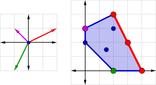
Figure 2.2: Left: Directions ω1,ω2,ω3\omega_{1},\omega_{2},\omega_{3}, and ω4=(0,0)\omega_{4}=(0,0). Right: The polytope Q⊂ℝ2Q\subset\mathbb{R}^{2} and three of its proper faces exposed by ω1,ω2\omega_{1},\omega_{2}, and ω3\omega_{3}.

The dimension of QQ is 22 and its codimension is 00. Let ω1=(−1,1),ω2=(2,1),ω3=(−1,−2)\omega_{1}=(-1,1),\omega_{2}=(2,1),\omega_{3}=(-1,-2), and ω4=(0,0)\omega_{4}=(0,0). Then

hQ​(ω1)=3,hQ​(ω2)=8,hQ​(ω3)=−2,hQ​(ω4)=0,h_{Q}(\omega_{1})=3,\quad h_{Q}(\omega_{2})=8,\quad h_{Q}(\omega_{3})=-2,\quad h_{Q}(\omega_{4})=0,

and the faces exposed by ω1,ω2,ω3\omega_{1},\omega_{2},\omega_{3}, and ω4\omega_{4} are

Qω1={(0,3)},Qω2=conv⁡({(2,4),(4,0)}),Qω3={(2,0)},Qω4=Q.Q_{\omega_{1}}=\{(0,3)\},\quad Q_{\omega_{2}}=\conv(\{(2,4),(4,0)\}),\quad Q_{\omega_{3}}=\{(2,0)\},\quad Q_{\omega_{4}}=Q.

Figure 2.2 depicts these directions and faces. In total, QQ has one empty face, five vertices, five facets (edges), and one 22-face. ⋄\diamond

Given a polytope P⊂ℝnP\subset\mathbb{R}^{n}, it is useful to collect directions ω∈ℝn\omega\in\mathbb{R}^{n} which expose the same face into cones. A subset C⊂ℝnC\subset\mathbb{R}^{n} is a cone if for any p∈Cp\in C, we have that λ​p∈C\lambda p\in C for λ∈ℝ≥0\lambda\in\mathbb{R}_{\geq 0}. A cone is a convex cone if it is closed under addition. Indeed if pp and qq are elements of a cone CC which is closed under addition and λ∈[0,1]\lambda\in[0,1] then λ​p+(1−λ)​q∈C\lambda p+(1-\lambda)q\in C since each summand is in CC. The (outer) normal fan of a polytope PP is the collection

𝒩⁡(P)={C⁡[ω]}ω∈ℝn{{{\color[rgb]{0,0,1}\mathcal{N}(P)}}}=\{C[\omega]\}_{\omega\in\mathbb{R}^{n}}

of convex cones

C⁡[ω]={ω′∈ℝn∣Pω⊆Pω′}.{{{\color[rgb]{0,0,1}C[\omega]}}}=\{\omega^{\prime}\in\mathbb{R}^{n}\mid P_{\omega}\subseteq P_{\omega^{\prime}}\}.

We denote the set of all C⁡[ω]C[\omega] of codimension at least ii by 𝒩(i)​(P)\mathcal{N}^{(i)}(P).

Example 2.1.5.

Figure 2.3 displays QQ along with its normal fan 𝒩⁡(Q)\mathcal{N}(Q) which has one zero-dimensional cone (the origin), five one-dimensional cones, and five two-dimensional cones. ⋄\diamond

Refer to caption
Figure 2.3: A polytope and its corresponding normal fan
Lemma 2.1.6.

[5, Proposition 2.2] Every polytope may be written as

P=conv⁡(vert⁡(P)).P=\conv(\vertices(P)). (2.1)

If 𝒜⊂ℝn\mathcal{A}\subset\mathbb{R}^{n} is finite, then vert⁡(conv⁡(𝒜))⊆𝒜\vertices(\conv(\mathcal{A}))\subseteq\mathcal{A}.

Lemma 2.1.7.

[5, Proposition 2.3] Let FF be a face of a polytope P⊂ℝnP\subset\mathbb{R}^{n}.

  1. (1)

    FF is a polytope with vert⁡(F)=F∩vert⁡(P)\vertices(F)=F\cap\vertices(P).

  2. (2)

    Every intersection of faces of PP is a face of PP.

  3. (3)

    The faces of FF are exactly the faces of PP that are contained in FF.

  4. (4)

    F=P∩ℝ​FF=P\cap\mathbb{R}F.

Lemma 2.1.6 gives one way to canonically represent a polytope: as the convex hull of its vertices. This representation is called the vertex representation of a polytope. Halfspaces provide another way to represent polytopes. A halfspace of ℝn\mathbb{R}^{n} is any subset of the form

ℝω,cn={x∈ℝn∣⟨x,ω⟩≤c}⊂ℝn,{{{\color[rgb]{0,0,1}\mathbb{R}^{n}_{\omega,c}}}}=\{x\in\mathbb{R}^{n}\mid\langle x,\omega\rangle\leq c\}\subset\mathbb{R}^{n},

for some ω∈ℝn\omega\in\mathbb{R}^{n} and c∈ℝc\in\mathbb{R}. Given a polytope P⊂ℝnP\subset\mathbb{R}^{n} and any direction ω∈ℝn\omega\in\mathbb{R}^{n}, the halfspace HP​(ω)=ℝω,hP​(ω)n{{{\color[rgb]{0,0,1}H_{P}(\omega)}}}=\mathbb{R}^{n}_{\omega,h_{P}(\omega)} contains PP. Note that HP​(ω)=HP​(λ⋅ω)H_{P}(\omega)=H_{P}(\lambda\cdot\omega) for any λ>0\lambda>0.

Lemma 2.1.8.

[5, Theorem 2.15] Every polytope P⊂ℝnP\subset\mathbb{R}^{n} may be written as

P=ℝ​P∩(⋂i=1mHP​(ωi))P=\mathbb{R}P\cap\left(\bigcap_{i=1}^{m}H_{P}(\omega_{i})\right) (2.2)

for any set {ωi}i=1m⊂ℝn\{\omega_{i}\}_{i=1}^{m}\subset\mathbb{R}^{n} such that {Pωi}i=1m=facets⁡(P)\{P_{\omega_{i}}\}_{i=1}^{m}=\facets(P). Conversely, any bounded intersection of halfspaces is a polytope.

If a polytope is nn-dimensional, then it has a unique representation of the form (2.2) since each facet is (n−1)(n-1)-dimensional and is exposed by its unique outer-normal ray. Note that these are the one-dimensional cones in the normal fan of a polytope. If a polytope has positive codimension, then it has a unique representation of the form (2.2) within its affine hull (the ωi\omega_{i} in (2.2) are taken to be parallel with the affine hull of PP). We call such a unique representation the halfspace representation of a polytope.

Example 2.1.9.

The polytope QQ in Example 2.1.3 has the halfspace representation,

Q=HQ​(2,1)∩HQ​(0,−1)∩HQ​(−1,−1)∩HQ​(−1,0)∩HQ​(−1,2).Q=H_{Q}(2,1)\cap H_{Q}(0,-1)\cap H_{Q}(-1,-1)\cap H_{Q}(-1,0)\cap H_{Q}(-1,2).

Each of these halfspaces are displayed in Figure 2.4.

Refer to caption
Figure 2.4: Five halfspaces in ℝ2\mathbb{R}^{2} whose intersection is QQ.

⋄\diamond

2.2  Oracles

While the vertex and halfspace representations are the most common ways of expressing a polytope, other representations come from functions called oracles. Colloquially, an oracle is an entity which provides prophetic insight whenever queried. Likewise, the vertex oracle for a polytope P⊂ℝnP\subset\mathbb{R}^{n} is the function

𝕍P:ℝn→ℝn∪{PFE}{\mathbb{V}}_{P}\colon\mathbb{R}^{n}\to\mathbb{R}^{n}\cup\{\texttt{PFE}\}
ω↦{Pωdim(Pω)=0PFEotherwise\omega\mapsto\begin{array}[]{cc}\left\{\begin{array}[]{lccl}P_{\omega}&&&\dim(P_{\omega})=0\\ \texttt{PFE}&&&\text{otherwise}\\ \end{array}\right.\end{array}

where PFE abbreviates the expression “Positive dimensional Face Exposed”. We remark that 𝕍P​(ω)=PFE\mathbb{V}_{P}(\omega)=\texttt{PFE} if and only if ω∈𝒩(1)​(P)\omega\in\mathcal{N}^{(1)}(P). The process of evaluating a vertex oracle is called querying the oracle.

Remark 2.2.1.

When a vertex oracle query returns a vertex 𝕍P​(ω)=v\mathbb{V}_{P}(\omega)=v, it implicitly returns the information that hP​(ω)=⟨v,ω⟩h_{P}(\omega)=\langle v,\omega\rangle and therefore that P⊂ℝω,⟨v,ω⟩n=HP​(ω)P\subset\mathbb{R}^{n}_{\omega,\langle v,\omega\rangle}=H_{P}(\omega).

Let 𝟎{{{\color[rgb]{0,0,1}{\boldsymbol{0}}}}} denote the all 00’s vector in ℝn\mathbb{R}^{n}, 𝟏{{{\color[rgb]{0,0,1}{\boldsymbol{1}}}}} denote the all 11’s vector in ℝn\mathbb{R}^{n}, and ei{{{\color[rgb]{0,0,1}e_{i}}}} denote the ii-th coordinate vector in ℝn\mathbb{R}^{n}. For any v∈ℝnv\in\mathbb{R}^{n}, let |v|{{{\color[rgb]{0,0,1}|v|}}} denote the sum of its coordinates. Given a polytope P⊂ℝnP\subset\mathbb{R}^{n}, let ℒ⁡(P)=P∩ℤn{{{\color[rgb]{0,0,1}\mathcal{L}(P)}}}=P\cap\mathbb{Z}^{n} denote its set of lattice points.

Proposition 2.2.2.

If P⊂ℝnP\subset\mathbb{R}^{n} is an integral polytope, then the vertex representation of PP can be recovered from the vertex oracle for PP.

Proof.

Let P⊂ℝnP\subset\mathbb{R}^{n} be an integral polytope and 𝕍P\mathbb{V}_{P} its vertex oracle. To prove the proposition, we first bound PP between two polytopes by querying the vertex oracle as follows.

Let ω∗=(ω1∗,…,ωn∗)∈ℝ>0n\omega^{*}=(\omega^{*}_{1},\ldots,\omega^{*}_{n})\in\mathbb{R}^{n}_{>0} be a vector such that ω1∗,…,ωn∗\omega^{*}_{1},\ldots,\omega^{*}_{n} are rationally independent (i.e. ⟨x,ω∗⟩≠0\langle x,\omega^{*}\rangle\neq 0 for any 𝟎≠x∈ℤn{\bf 0}\neq x\in\mathbb{Z}^{n}). Observe that 𝕍P​(ω∗)\mathbb{V}_{P}(\omega^{*}) must return a vertex: otherwise, there exist two vertices p1,p2p_{1},p_{2} such that ⟨p1,ω∗⟩=⟨p2,ω∗⟩\langle p_{1},\omega^{*}\rangle=\langle p_{2},\omega^{*}\rangle implying that x=p1−p2x=p_{1}-p_{2} is an integer point whose dot product with ω∗\omega^{*} is nonzero. A consequence of Remark 2.2.1 is that the halfspace HP​(ω∗)H_{P}(\omega^{*}) containing PP is computed as well. Since ω\omega is in the positive orthant, HP​(ω∗)H_{P}(\omega^{*}) bounds P∩ℝ≥0nP\cap\mathbb{R}^{n}_{\geq 0}.

Similarly, for every vertex vv of the hypercube cube​(n)=[−1,1]n{{{\color[rgb]{0,0,1}\text{cube}(n)}}}=[-1,1]^{n}, we let v∘ω∗v\circ\omega^{*} denote the Hadamard (coordinate-wise) product so that the output 𝕍P​(v∘ω∗)\mathbb{V}_{P}(v\circ\omega^{*}) is a vertex of PP. Again, each oracle query bounds PP in the corresponding orthant of ℝn\mathbb{R}^{n} so that the intersection

P∗=⋂v∈cube​(n)HP​(v∘ω∗),P^{*}=\bigcap_{v\in\text{cube}(n)}H_{P}(v\circ\omega^{*}),

is bounded, and thus by Lemma 2.1.8, is a polytope. Setting P∗=conv⁡({𝕍P​(v∘ω)∣v∈cube​(n)})P_{*}=\conv(\{\mathbb{V}_{P}(v\circ\omega)\mid v\in\text{cube}(n)\}) gives containments

P∗⊆P⊆P∗.P_{*}\subseteq P\subseteq P^{*}. (2.3)

The proof proceeds algorithmically. Set P∗=conv⁡(ℒ⁡(P∗))P^{*}=\conv\left(\mathcal{L}(P^{*})\right) so that P∗P^{*} is integral. Since PP is integral, the containments (2.3) are still true. For every p∈vert⁡(P∗)∖P∗p\in\vertices(P^{*})\smallsetminus P_{*}, pick ω\omega such that 𝕍P∗​(ω)=p\mathbb{V}_{P^{*}}(\omega)=p. Since pp is the unique point in P∗P^{*} obtaining a maximum dot product with ω\omega and P⊆P∗P\subseteq P^{*} then p∈Pp\in P if and only if 𝕍P​(ω)=p\mathbb{V}_{P}(\omega)=p. We have three cases: either p∈Pp\in P and so 𝕍P​(ω)=p\mathbb{V}_{P}(\omega)=p (case (i)), or 𝕍P​(ω)\mathbb{V}_{P}(\omega) returns PFE (case (ii)) or 𝕍P​(ω)\mathbb{V}_{P}(\omega) returns another vertex q≠pq\neq p (case (iii)).

Case (i): If 𝕍P​(ω)=p\mathbb{V}_{P}(\omega)=p then set P∗=conv⁡(P∗∪p)P_{*}=\conv(P_{*}\cup p). Note that the containments (2.3) still hold and that the number of lattice points of P∗P_{*} has increased.

Case (ii): If 𝕍P​(ω)=PFE\mathbb{V}_{P}(\omega)=\texttt{PFE}, then p∉Pp\not\in P and so we may set P∗=conv⁡(ℒ⁡(P∗)∖p)P^{*}=\conv(\mathcal{L}(P^{*})\smallsetminus p) while preserving (2.3). In this case, the number of lattice points of P∗P^{*} has decreased.

Case (iii): If 𝕍P​(ω)=q≠p\mathbb{V}_{P}(\omega)=q\neq p, then we may set P∗=conv⁡(P∗∪q)P_{*}=\conv(P_{*}\cup q) and P∗=conv⁡(ℒ⁡(P∗∩HP​(ω)))P^{*}=\conv(\mathcal{L}(P^{*}\cap H_{P}(\omega))) while preserving (2.3). In this case, the number of lattice points of P∗P_{*} may have increased depending on whether or not qq was already in P∗P_{*}, but it will always be the case that the number of lattice points of P∗P^{*} has decreased.

Each oracle query involves one of the above cases and each case preserves the containments (2.3) while either increasing the number of lattice points in P∗P_{*} or decreasing the number of lattice points in P∗P^{*}. Thus, this process must terminate with vert⁡(P∗)∖P∗=∅\vertices(P^{*})\smallsetminus P_{*}=\emptyset, proving that these polytopes are equal to each other and so P∗=P=P∗P_{*}=P=P^{*}. ∎

.

Algorithm 2.2.3 (Vertex oracle →\to vertex representation).
.
Input:
∙\bullet The vertex oracle 𝕍P\mathbb{V}_{P} for an integral polytope P⊂ℝ≥0nP\subset\mathbb{R}^{n}_{\geq 0}
Output:
∙\bullet
The vertex representation for PP
Steps:
0 Pick ω∗=(ω1∗,…,ωn∗)∈ℝ>0n\omega^{*}=(\omega_{1}^{*},\ldots,\omega^{*}_{n})\in\mathbb{R}^{n}_{>0} with rationally independent coordinates 1 set P∗=∅P_{*}=\emptyset, set P∗=ℝnP^{*}=\mathbb{R}^{n} 2 for each vertex v∈cube​(n)v\in\text{cube}(n) do 2.1 set P∗=conv⁡(P∗∪𝕍P​(v∘ω∗))P_{*}=\conv(P_{*}\cup\mathbb{V}_{P}(v\circ\omega^{*})) 2.2 set P∗=P∗∩HP​(v∘ω∗)P^{*}=P^{*}\cap H_{P}(v\circ\omega^{*}) 3 while ℒ⁡(P∗)≠ℒ⁡(P∗)\mathcal{L}(P_{*})\neq\mathcal{L}(P^{*}) do 3.1 set P∗=conv⁡(ℒ⁡(P∗))P^{*}=\conv(\mathcal{L}(P^{*})) 3.2 Pick p∈vert⁡(P∗)∖P∗p\in\vertices(P^{*})\smallsetminus P_{*} 3.3 Find ω∈ℝn\omega\in\mathbb{R}^{n} such that 𝕍P∗​(ω)=p\mathbb{V}_{P^{*}}(\omega)=p 3.4 if 𝕍P​(ω)=p\mathbb{V}_{P}(\omega)=p then set P∗=conv⁡(P∗∪p)P_{*}=\conv(P_{*}\cup p) 3.5 if 𝕍P​(ω)=PFE\mathbb{V}_{P}(\omega)=\texttt{PFE} then set P∗=conv⁡(ℒ⁡(P∗)∖p)P^{*}=\conv(\mathcal{L}(P^{*})\smallsetminus p) 3.6 if 𝕍P​(ω)=q≠p\mathbb{V}_{P}(\omega)=q\neq p then 3.6.1 set P∗=P∗∩HP​(ω)P^{*}=P^{*}\cap H_{P}(\omega) 3.6.2 if q∉P∗q\not\in P_{*} then set P∗=conv⁡(P∗∪p)P_{*}=\conv(P_{*}\cup p) 4 return vert⁡(P∗)\vertices(P_{*})

.

Example 2.2.4.

Figure 2.5 displays the steps required to complete Algorithm 2.2.3 on QQ from Example 2.1.3. We use ω∗=(1,2)\omega^{*}=(1,\sqrt{2}) in step (0)(0) of the algorithm. Step (2)(2) in Algorithm 2.2.3 is represented by the top-left graphic showing the four vertex oracle queries on the vectors ω∗,−ω∗,(−1,2),\omega^{*},-\omega^{*},(-1,\sqrt{2}), and (1,−2)(1,-\sqrt{2}). Each query reveals a vertex of QQ and a halfspace containing QQ. The intersection of all such halfspaces Q∗Q^{*} is depicted in grey in the first image along with Q∗Q_{*} in green and conv⁡(ℒ⁡(Q∗))\conv(\mathcal{L}(Q^{*})) in red.

Refer to caption
Figure 2.5: A graphical interpretation of Algorithm 2.2.3 running on the polytope QQ in Example 2.1.3.

The next image (to the right) displays the oracle query 𝕍Q​(1,0)=(4,0)\mathbb{V}_{Q}(1,0)=(4,0), revealing a vertex which was already found. Thus, this oracle query does not increase the size of Q∗Q_{*} but it does establish that (5,1)(5,1) (a previous vertex of Q∗Q^{*}) is not contained in QQ and so the size of Q∗Q^{*} is reduced. The third image (bottom left) attempts to establish whether or not (4,2)∈Q(4,2)\in Q by choosing ω=(2,1)\omega=(2,1) so that 𝕍Q∗​(ω)=(4,2)\mathbb{V}_{Q^{*}}(\omega)=(4,2) and querying 𝕍Q​(ω)=PFE\mathbb{V}_{Q}(\omega)=\texttt{PFE}. This does not find a new vertex of QQ, nor does it find a new halfspace containing QQ. It does, however, reveal that (4,2)∉Q(4,2)\not\in Q and so Q∗Q^{*} is again reduced to conv⁡(ℒ⁡(Q∗)∖(4,2))\conv(\mathcal{L}(Q^{*})\smallsetminus(4,2)). At this stage, (0,2)(0,2) is the unique vertex of Q∗Q^{*} which is not in Q∗Q_{*} and 𝕍Q​(−2,1)=(0,2)\mathbb{V}_{Q}(-2,1)=(0,2) reveals that it is a vertex of QQ. The outer polytope Q∗Q^{*} is reduced again, the inner polytope Q∗Q_{*} grows, and Q∗Q^{*} becomes equal to Q∗Q_{*}, ending the algorithm. ⋄\diamond

Remark 2.2.5.

Implementing Algorithm 2.2.3, as is, requires the representation of a rationally independent vector ω∗\omega^{*} on a computer for step (2)(2). Theoretically, a random ω∈ℝn\omega\in\mathbb{R}^{n} will expose a vertex of PP with probability one and so in practice, we replace steps (0)(0) and (2)(2) by randomly querying the oracle in each orthant until a vertex is returned. This process bounds PP in a polytope P∗P^{*}. We remark that probability one statements about the theory may not translate to probability one computations and we give a more detailed discussion in Remark 7.3.3 in Section 7. ⋄\diamond

We denote the standard full-dimensional simplex in ℝn\mathbb{R}^{n} by Δn=conv⁡(𝟎,e1,…,en){{{\color[rgb]{0,0,1}\Delta_{n}}}}=\conv({\boldsymbol{0}},e_{1},\ldots,e_{n}) and the dilation of Δn\Delta_{n} by a factor of dd by d​Δn=conv⁡(𝟎,d⋅e1,…,d⋅en){{{\color[rgb]{0,0,1}d\Delta_{n}}}}=\conv({\boldsymbol{0}},d\cdot e_{1},\ldots,d\cdot e_{n}). The degree of a polytope P⊂ℝ≥0nP\subset\mathbb{R}_{\geq 0}^{n}, is deg⁡(P)\deg(P)=hP​(𝟏)=h_{P}({\bf 1}). A polytope is homogeneous if |p|=deg⁡(P)|p|=\deg(P) for all p∈Pp\in P and the homogenization of PP is P~={(p,deg⁡(P)−|p|)∣p∈P}⊂ℝn+1{{{\color[rgb]{0,0,1}\widetilde{P}}}}=\{(p,\deg(P)-|p|)\mid p\in P\}\subset\mathbb{R}^{n+1}.

Definition 2.2.6.

The numerical oracle for a polytope P∈ℝnP\in\mathbb{R}^{n} is the function

𝒪P:ℝn→ℝn∪{EEP}{\mathcal{O}}_{P}\colon\mathbb{R}^{n}\to\mathbb{R}^{n}\cup\{\texttt{EEP}\}
ω↦{Pωdim(Pω)=0min⁡(Pω)0<dim(Pω)<dim(P)EEPPω=P\omega\mapsto\begin{array}[]{ll}\left\{\begin{array}[]{llll}P_{\omega}&&&\dim(P_{\omega})=0\\ \min(P_{\omega})&&&0<\dim(P_{\omega})<\dim(P)\\ \texttt{EEP}&&&P_{\omega}=P\\ \end{array}\right.\end{array}

where min⁡(Pω)\min(P_{\omega}) is the coordinate-wise minimum of all points in PωP_{\omega}.

The expression EEP abbreviates Exposes Entire Polytope. This oracle is dubbed “numerical” because it arises naturally from the numerical HS-algorithm (Algorithm 7.1.2 of Section 7).

Generally, one cannot distinguish whether the output of a numerical oracle for a polytope PP is a vertex v=Pωv=P_{\omega} or the coordinate-wise minimum w=min⁡(Pω)w=\min(P_{\omega}) of a positive-dimensional face. For example, the numerical oracle query 𝒪Δ2​(1,1)\mathcal{O}_{\Delta_{2}}(1,1) returns 𝟎{\bf 0} not because 𝟎{\bf 0} is a vertex, but because 𝟎=min⁡(conv⁡(e1,e2)){\bf 0}=\min(\conv(e_{1},e_{2})). Thus, at first glance, a numerical oracle may seem weaker than a vertex oracle. However, when the polytope PP is homogeneous of degree dd these cases may be distinguished easily since the sum of the coordinates of a vector output of 𝒪P​(ω)\mathcal{O}_{P}(\omega) will be dd if and only if the vector is a vertex and it will be less than dd otherwise. Restricted to homogeneous polytopes, a numerical oracle gives strictly more information than a vertex oracle, implying the following corollary to Proposition 2.2.2.

Corollary 2.2.7.

If PP is a homogeneous integral polytope then the vertex representation of PP may be recovered from its numerical oracle.

Other oracles for polytopes exist and are well-studied. For example, Emiris et. al. [6] developed an algorithm similar to Algorithm 2.2.3 for oracles which are stronger than vertex oracles: instead of returning PFE, they return a vertex on the corresponding positive-dimensional face.

2.3  Mixed volume

We develop some of the theory of mixed volumes of polytopes and include multiple formulas and characterizations of mixed volume. We list them here for convenience.

  1. (1)

    Coefficient of a volume function (Definition 2.3.3).

  2. (2)

    Volume alternating sum formula (Lemma 2.3.6).

  3. (3)

    Axiomatic characterization (Lemma 2.3.8).

  4. (4)

    Lattice point alternating sum formula for integral polytopes (Lemma 2.3.9).

  5. (5)

    Sum of volumes of mixed cells formula (Lemma 2.4.3).

We give a sixth way of computing mixed volume in Section 5 via the Bernstein-Kushnirenko Theorem (Proposition 5.3.1).

We begin our discussion by introducing two natural operations on subsets of ℝn\mathbb{R}^{n}. Let S1,S2⊂ℝnS_{1},S_{2}\subset\mathbb{R}^{n} and λ∈ℝ≥0\lambda\in\mathbb{R}_{\geq 0}. The set

λ​S1={λ​s∣s∈S1},{{{\color[rgb]{0,0,1}\lambda S_{1}}}}=\{\lambda s\mid s\in S_{1}\},

is the scaling of S1S_{1} by λ\lambda. The set

S1+S2={s1+s2∣s1∈S1,s2∈S2},{{{\color[rgb]{0,0,1}S_{1}+S_{2}}}}=\{s_{1}+s_{2}\mid s_{1}\in S_{1},s_{2}\in S_{2}\},

is the Minkowski sum of S1S_{1} and S2S_{2}. The scaling of a polytope P=conv⁡(𝒜)P=\conv(\mathcal{A}) by λ∈ℝ≥0\lambda\in\mathbb{R}_{\geq 0} is clearly a polytope given as λ​P=conv⁡(λ​𝒜)\lambda P=\conv(\lambda\mathcal{A}). The following lemma proves an analogous result for Minkowski sums of polytopes.

Lemma 2.3.1.

Let P,Q⊂ℝnP,Q\subset\mathbb{R}^{n} be polytopes.

  1. (1)

    The support functions of PP and QQ are additive: hP+Q=hP+hQh_{P+Q}=h_{P}+h_{Q}.

  2. (2)

    The Minkowski sum P+QP+Q is a polytope which may be written as conv⁡(vert⁡(P)+vert⁡(Q))\conv(\vertices(P)+\vertices(Q)).

  3. (3)

    If F⊂P+QF\subset P+Q is a face, then there exist unique faces FP⊆PF_{P}\subseteq P and FQ⊆QF_{Q}\subseteq Q such that F=FP+FQF=F_{P}+F_{Q}.

  4. (4)

    If PP and QQ are integral, so is P+QP+Q.

Proof.

Additivity of support functions is immediate since

hP+Q​(ω)=maxs∈P+Q⁡⟨s,ω⟩=maxp∈P,q∈Q⁡⟨p+q,ω⟩=maxp∈P⁡⟨p,ω⟩+maxq∈Q⁡⟨q,ω⟩.h_{P+Q}(\omega)=\max_{s\in P+Q}\langle s,\omega\rangle=\max_{p\in P,q\in Q}\langle p+q,\omega\rangle=\max_{p\in P}\langle p,\omega\rangle+\max_{q\in Q}\langle q,\omega\rangle.

To show that P+QP+Q is a polytope, we first show P+QP+Q is convex. Let a=p1+q1a=p_{1}+q_{1} and b=p2+q2b=p_{2}+q_{2} for p1,p2∈Pp_{1},p_{2}\in P and q1,q2∈Qq_{1},q_{2}\in Q. Then v∈[a,b]v\in[a,b] implies

v\displaystyle v =λ​a+(1−λ)​b\displaystyle=\lambda a+(1-\lambda)b
=λ⁡(p1+q1)+(1−λ)​(p2+q2)\displaystyle=\lambda(p_{1}+q_{1})+(1-\lambda)(p_{2}+q_{2})
=(λ​p1+(1−λ​p2))+(λ​q1+(1−λ)​q2)∈P+Q,\displaystyle=(\lambda p_{1}+(1-\lambda p_{2}))+(\lambda q_{1}+(1-\lambda)q_{2})\in P+Q,

proving that P+QP+Q is convex. To see that P+Q⊂conv⁡(vert⁡(P)+vert⁡(Q))P+Q\subset\conv(\vertices(P)+\vertices(Q)), suppose towards contradiction that there exists v∈P+Q∖conv⁡(vert⁡(P)+vert⁡(Q))v\in P+Q\smallsetminus\conv(\vertices(P)+\vertices(Q)). Then there exists a halfspace of conv⁡(vert⁡(P)+vert⁡(Q))\conv(\vertices(P)+\vertices(Q)) not containing vv. In other words, there exists ω\omega such that ⟨v,ω⟩=hP+Q​(ω)>hP​(ω)+hQ​(ω)\langle v,\omega\rangle=h_{P+Q}(\omega)>h_{P}(\omega)+h_{Q}(\omega), a contradiction by part (1)(1). Thus,

vert⁡(P)+vert⁡(Q)⊂P+Q⊂conv⁡(vert⁡(P)+vert⁡(Q)),\vertices(P)+\vertices(Q)\subset P+Q\subset\conv(\vertices(P)+\vertices(Q)),

and taking the convex hull of this containment proves parts (2)(2) and (4)(4).

To prove part (3)(3), observe that for any ω∈ℝn\omega\in\mathbb{R}^{n} we have (P+Q)ω=Pω+Qω(P+Q)_{\omega}=P_{\omega}+Q_{\omega} by part (1)(1). Suppose

(P+Q)ω=Pω′+Qω′′,(P+Q)_{\omega}=P_{\omega^{\prime}}+Q_{\omega^{\prime\prime}},

for some other ω′,ω′′∈ℝn\omega^{\prime},\omega^{\prime\prime}\in\mathbb{R}^{n}. The evaluation of x↦⟨x,ω⟩x\mapsto\langle x,\omega\rangle at any point on the right-hand-side must equal hP​(ω)+hQ​(ω)h_{P}(\omega)+h_{Q}(\omega), implying that Pω′=PωP_{\omega^{\prime}}=P_{\omega} and Qω′′=QωQ_{\omega^{\prime\prime}}=Q_{\omega}. ∎

To fix notation, let P∙={P1,…,Pn}{{{\color[rgb]{0,0,1}P_{\bullet}}}}=\{P_{1},\ldots,P_{n}\} be a collection of nn polytopes in ℝn\mathbb{R}^{n}. We denote the set {1,…,n}\{1,\ldots,n\} by [n]{{{\color[rgb]{0,0,1}[n]}}}. The following result is due to Minkowski when d=3d=3 [7].

Lemma 2.3.2 (H. Minkowski [7]).

The function

V⁡(P∙):ℝ≥0n→ℝ{{{\color[rgb]{0,0,1}V(P_{\bullet})}}}\colon\mathbb{R}^{n}_{\geq 0}\to\mathbb{R}
V⁡(P∙)​(λ1,…,λn)=vol⁡(λ1​P1+⋯+λn​Pn)V(P_{\bullet})(\lambda_{1},\ldots,\lambda_{n})=\vol(\lambda_{1}P_{1}+\cdots+\lambda_{n}P_{n})

is a homogeneous polynomial of degree nn in ℝ⁡[λ1,…,λn]\mathbb{R}[\lambda_{1},\ldots,\lambda_{n}] where vol{{{\color[rgb]{0,0,1}\vol}}} denotes the nn-dimensional Euclidean volume.

Definition 2.3.3.

The mixed volume of P∙P_{\bullet}, denoted MV⁡(P∙){{{\color[rgb]{0,0,1}\MV(P_{\bullet})}}}, is the coefficient of λ1λ2⋯λn\lambda_{1}\lambda_{2}\cdots\lambda_{n} in V⁡(P∙)V(P_{\bullet}).

Example 2.3.4.

Consider A=conv⁡(𝟎,e1,e2,e1+e2)A=\conv({\boldsymbol{0}},e_{1},e_{2},e_{1}+e_{2}) and B=conv⁡(𝟎,e1,e2)B=\conv({\boldsymbol{0}},e_{1},e_{2}) as displayed in Figure 2.6. Then V⁡(A,B)=λ12+2​λ1​λ2+12​λ22V(A,B)=\lambda_{1}^{2}+2\lambda_{1}\lambda_{2}+\frac{1}{2}\lambda_{2}^{2} and so MV⁡(A,B)=2\MV(A,B)=2.

Refer to caption
Figure 2.6: A graphic expressing vol​(λ1​A+λ2​B)\text{vol}(\lambda_{1}A+\lambda_{2}B) for two polygons A,B⊂ℝ2A,B\subset\mathbb{R}^{2}.

⋄\diamond

Lemma 2.3.5.

Let P,P1,…,Pn,Q⊂ℝnP,P_{1},\ldots,P_{n},Q\subset\mathbb{R}^{n} be polytopes and let a∈ℝ≥0a\in\mathbb{R}_{\geq 0}. Then,

  1. (1)

    MV⁡(P,…,P)=n!​vol⁡(P)\MV(P,\ldots,P)=n!\vol(P).

  2. (2)

    MV\MV is symmetric in its arguments.

  3. (3)

    MV\MV is multilinear:

    MV⁡(a​P1+Q,P2,…,Pn)=a​MV⁡(P1,…,Pn)+MV⁡(Q,P2,…,Pn).\MV(aP_{1}+Q,P_{2},\ldots,P_{n})=a\MV(P_{1},\ldots,P_{n})+\MV(Q,P_{2},\ldots,P_{n}).
Proof.

Note that vol⁡(λ1​P+⋯+λn​P)=vol⁡((λ1+⋯+λn)​P)=(λ1+⋯+λn)n​vol⁡(P)\vol(\lambda_{1}P+\cdots+\lambda_{n}P)=\vol((\lambda_{1}+\cdots+\lambda_{n})P)=(\lambda_{1}+\cdots+\lambda_{n})^{n}\vol(P) and so the coefficient of λ1⋯λn\lambda_{1}\cdots\lambda_{n} is n!​vol⁡(P)n!\vol(P). Part (2)(2) is immediate from the definition of mixed volume. For a proof of part (3)(3), see [8, Lemma 3.6]. ∎

Lemma 2.3.6.

[8, Theorem 3.7] Given a collection of polytopes P1,…,PnP_{1},\ldots,P_{n},

MV⁡(P1,…,Pn)=∑I⊂[n](−1)n−|I|​vol⁡(∑i∈IPi).\MV(P_{1},\ldots,P_{n})=\sum_{I\subset[n]}(-1)^{n-|I|}\vol\left(\sum_{i\in I}P_{i}\right).
Proof.

We restate the proof given in [8]. Due to precisely the properties of mixed volume in Lemma 2.3.5, we may treat the statement in the theorem as the polynomial equation

n!x1⋯xn=(x1+⋯+xn)n−∑i=1n(x1+⋯+xi−1+xi+1+⋯xn)n+−⋯n!x_{1}\cdots x_{n}=(x_{1}+\cdots+x_{n})^{n}-\sum_{i=1}^{n}(x_{1}+\cdots+x_{i-1}+x_{i+1}+\cdots x_{n})^{n}+-\cdots (2.4)
⋯+(−1)n−2​∑i<j(xi+xj)n+(−1)n−1​∑i=1nxin,\cdots+(-1)^{n-2}\sum_{i<j}(x_{i}+x_{j})^{n}+(-1)^{n-1}\sum_{i=1}^{n}x_{i}^{n},

where xi1⋯xiN↔vol(λi1⋅Pi1+⋯+λiN⋅PiN)x_{i_{1}}\cdots x_{i_{N}}\leftrightarrow\vol\left(\lambda_{i_{1}}\cdot P_{i_{1}}+\cdots+\lambda_{i_{N}}\cdot P_{i_{N}}\right). To verify (2.4), we may simply check how many times each monomial appears in the right-hand-side. The monomial xinx_{i}^{n} appears once in the first term, n−1n-1 times in the second, and so on to give a total of

1−(n−1)+(n−12)−⋯+(−1)n−2​(n−1)+(−1)n−1=(1−1)n−1=0.1-(n-1)+{{n-1}\choose{2}}-\cdots+(-1)^{n-2}(n-1)+(-1)^{n-1}=(1-1)^{n-1}=0.

Similarly, every term on the right-hand-side cancels except for the mixed term x1⋯xnx_{1}\cdots x_{n} which appears n!n! times. ∎

Since the formula in Lemma 2.3.6 is short when n=2n=2, we state it as a corollary.

Corollary 2.3.7.

The mixed volume of two convex polygons P1,P2⊂ℝ2P_{1},P_{2}\subset\mathbb{R}^{2} is

MV⁡(P1,P2)=vol⁡(P1+P2)−vol⁡(P1)−vol⁡(P2).\MV(P_{1},P_{2})=\vol(P_{1}+P_{2})-\vol(P_{1})-\vol(P_{2}).
Lemma 2.3.8.

The only function from nn-tuples of polytopes to ℝ\mathbb{R} satisfying the properties in Lemma 2.3.5 is MV\MV.

Proof.

The proof of the formula of Lemma 2.3.6 relied precisely on the properties in Lemma 2.3.5. Thus, any other function satisfying those properties will have the same formula. ∎

When each polytope in a collection P∙P_{\bullet} is integral, there is a discrete analog of Lemma 2.3.6 involving lattice point enumeration.

Lemma 2.3.9.

[9, Corollary 3.10] Given a collection of integral polytopes P1,…,PnP_{1},\ldots,P_{n},

MV⁡(P1,…,Pn)=(−1)n+∑∅≠I⊂[n](−1)n−|I|​|ℒ⁡(∑i∈IPi)|.\MV(P_{1},\ldots,P_{n})=(-1)^{n}+\sum_{\emptyset\neq I\subset[n]}(-1)^{n-|I|}\Bigl|\mathcal{L}\Bigl(\sum_{i\in I}P_{i}\Bigr)\Bigr|.

2.4  Subdivisions

Following [2] we give the notion of subdivisions of collections of finite subsets of ℝn\mathbb{R}^{n}. The combinatorial constructions in this section provide a fifth description of the mixed volume of a collection of polytopes and are fundamentally important for Algorithm 6.3.5 of Section 6.3.3.

Let 𝒜∙=(𝒜1,…,𝒜k){{{\color[rgb]{0,0,1}{\mathcal{A}_{\bullet}}}}}=(\mathcal{A}_{1},\ldots,\mathcal{A}_{k}) be a collection of finite subsets of ℝn\mathbb{R}^{n} whose union affinely spans ℝn\mathbb{R}^{n}. A cell of 𝒜∙{\mathcal{A}_{\bullet}} is a tuple 𝒞∙=(𝒞1,…,𝒞k)\mathcal{C}_{\bullet}=(\mathcal{C}_{1},\ldots,\mathcal{C}_{k}) of nonempty subset 𝒞i⊂𝒜i\mathcal{C}_{i}\subset\mathcal{A}_{i}. We define

type⁡(𝒞∙)\displaystyle{{{\color[rgb]{0,0,1}\type(\mathcal{C}_{\bullet})}}} =(dim(conv⁡(𝒞1)),…,dim(conv⁡(𝒞k))),\displaystyle=(\dim(\conv(\mathcal{C}_{1})),\ldots,\dim(\conv(\mathcal{C}_{k}))),
conv⁡(𝒞∙)\displaystyle{{{\color[rgb]{0,0,1}\conv(\mathcal{C}_{\bullet})}}} =conv⁡(𝒞1+⋯+𝒞k),\displaystyle=\conv(\mathcal{C}_{1}+\cdots+\mathcal{C}_{k}),
|𝒞∙|\displaystyle{{{\color[rgb]{0,0,1}|\mathcal{C}_{\bullet}|}}} =|𝒞1|+|𝒞2|+⋯+|𝒞k|,\displaystyle=|\mathcal{C}_{1}|+|\mathcal{C}_{2}|+\cdots+|\mathcal{C}_{k}|,
vol⁡(𝒞∙)\displaystyle{{{\color[rgb]{0,0,1}\vol(\mathcal{C}_{\bullet})}}} =vol⁡(conv⁡(𝒞∙)).\displaystyle=\vol(\conv(\mathcal{C}_{\bullet})).
Definition 2.4.1.

A subdivision of 𝒜∙{\mathcal{A}_{\bullet}} is a collection S∙={𝒞∙(1),…,𝒞∙(m)}S^{\bullet}=\left\{{\mathcal{C}}_{\bullet}^{(1)},\ldots,{\mathcal{C}}_{\bullet}^{(m)}\right\} of cells satisfying

  1. (1)

    dim(conv⁡(𝒞∙(i)))=n\dim\left(\conv\left({\mathcal{C}}_{\bullet}^{(i)}\right)\right)=n for all i=1,…,mi=1,\ldots,m.

  2. (2)

    conv⁡(𝒞∙(i))∩conv⁡(𝒞∙(j))\conv\left({\mathcal{C}}_{\bullet}^{(i)}\right)\cap\conv\left({\mathcal{C}}_{\bullet}^{(j)}\right) is a proper face of conv⁡(𝒞∙(i))\conv\left({\mathcal{C}}_{\bullet}^{(i)}\right) and conv⁡(𝒞∙(j))\conv\left({\mathcal{C}}_{\bullet}^{(j)}\right) for all i≠j∈[m]i\neq j\in[m].

  3. (3)

    ⋃i=1mconv⁡(𝒞∙(i))=conv⁡(𝒜∙).\bigcup_{i=1}^{m}\conv\left({\mathcal{C}}_{\bullet}^{(i)}\right)=\conv({\mathcal{A}_{\bullet}}).

If S∙S^{\bullet} additionally satisfies

  • (4)

    |type⁡(𝒞∙(i))|=n\left|\type\left({\mathcal{C}}_{\bullet}^{(i)}\right)\right|=n for all i=1,…,mi=1,\ldots,m,

then we say it is a mixed subdivision. Even stronger, if S∙S^{\bullet} additionally satisfies

  • (5)

    ∑i=1k(|𝒞i(j)|−1)=n\sum_{i=1}^{k}\left(\left|\mathcal{C}^{(j)}_{i}\right|-1\right)=n for all j=1,…,mj=1,\ldots,m,

then we say it is a fine mixed subdivision.

A cell 𝒞∙\mathcal{C}_{\bullet} of a subdivision S∙S^{\bullet} is called a mixed cell when min⁡(type⁡(𝒞∙))>0\min(\type(\mathcal{C}_{\bullet}))>0 and a fine mixed cell if it additionally satisfies ∑i=1k(|𝒞i|−1)=n\sum_{i=1}^{k}(|\mathcal{C}_{i}|-1)=n. When k=nk=n, a cell 𝒞∙\mathcal{C}_{\bullet} is mixed if type⁡(𝒞∙)=𝟏\type(\mathcal{C}_{\bullet})={\boldsymbol{1}} and it is fine mixed if |𝒞i|=2|\mathcal{C}_{i}|=2 for i=1,…,ki=1,\ldots,k.

Example 2.4.2.

When k=1k=1, every subdivision of 𝒜∙{\mathcal{A}_{\bullet}} is a mixed subdivision because parts (1)(1) and (4)(4) of Definition 2.4.1 become the same statement. The fine mixed subdivisions of 𝒜∙{\mathcal{A}_{\bullet}} are those with the property that the convex hull of each cell is an nn-simplex. Such subdivisions comprise a rich family of combinatorial objects called triangulations [10]. ⋄\diamond

The definitions above provide a new description of mixed volume.

Lemma 2.4.3.

[2, Theorem 2.4] Suppose 𝒜∙=(𝒜1,…,𝒜k){\mathcal{A}_{\bullet}}=(\mathcal{A}_{1},\ldots,\mathcal{A}_{k}) is a collection of finite subsets of ℝn\mathbb{R}^{n} whose union affinely spans ℝn\mathbb{R}^{n} and let Pi=conv⁡(𝒜i)P_{i}=\conv(\mathcal{A}_{i}). If S∙S^{\bullet} is a mixed subdivision of 𝒜∙{\mathcal{A}_{\bullet}} and r=(r1,…,rk)⊂ℕkr=(r_{1},\ldots,r_{k})\subset\mathbb{N}^{k} such that |r|=n|r|=n, then the mixed volume of

P=(P1,…,P1⏟r1,P2,…,P2⏟r2,…,Pk,…,Pk⏟rk),P=(\underbrace{P_{1},\ldots,P_{1}}_{r_{1}},\underbrace{P_{2},\ldots,P_{2}}_{r_{2}},\ldots,\underbrace{P_{k},\ldots,P_{k}}_{r_{k}}),

is the sum of the volumes of the mixed cells in S∙S^{\bullet} of type (r1,r2,…,rk)(r_{1},r_{2},\ldots,r_{k}):

MV⁡(P)=∑𝒞∙∈S∙type⁡(𝒞∙)=(r1,…,rk)vol⁡(𝒞∙).\MV(P)=\sum_{\begin{subarray}{c}{\mathcal{C}}_{\bullet}\in S^{\bullet}\\ \type({\mathcal{C}}_{\bullet})=(r_{1},\ldots,r_{k})\end{subarray}}\vol(\mathcal{C}_{\bullet}).

We describe a process which produces subdivisions from functions. Let 𝒜⊂ℝn\mathcal{A}\subset\mathbb{R}^{n} be a finite set and let ℓ:𝒜→ℝ\ell\colon\mathcal{A}\to\mathbb{R} be any function. Let Γℓ:𝒜→ℝn+1{{{\color[rgb]{0,0,1}\Gamma_{\ell}}}}\colon\mathcal{A}\to\mathbb{R}^{n+1} be the function Γℓ​(α)=(α,ℓ⁡(α)){\Gamma_{\ell}}(\alpha)=(\alpha,\ell(\alpha)). We call ℓ\ell a lifting function and we call the polytope

convℓ⁡(𝒜)=conv⁡(Γℓ​(𝒜))⊂ℝn+1,{{{\color[rgb]{0,0,1}\conv_{\ell}(\mathcal{A})}}}=\conv(\Gamma_{\ell}(\mathcal{A}))\subset\mathbb{R}^{n+1},

the lift of 𝒜\mathcal{A} by ℓ\ell. Similarly, given a set of functions ℓ∙=(ℓ1,…,ℓk){{{\color[rgb]{0,0,1}\ell_{\bullet}}}}=(\ell_{1},\ldots,\ell_{k}) with ℓi:𝒜i→ℝ\ell_{i}\colon\mathcal{A}_{i}\to\mathbb{R}, let Γℓ∙:𝒜∙→ℝn+1{{{\color[rgb]{0,0,1}\Gamma_{\ell_{\bullet}}}}}\colon{\mathcal{A}_{\bullet}}\to\mathbb{R}^{n+1} be the function Γℓ∙​(α1,…,αk)=∑i=1kΓℓi​(αi)\Gamma_{\ell_{\bullet}}(\alpha_{1},\ldots,\alpha_{k})=\sum_{i=1}^{k}\Gamma_{\ell_{i}}(\alpha_{i}). Analogously, define

convℓ∙⁡(𝒜∙)=conv⁡(Γℓ∙​(𝒜∙))=∑i=1kconvℓi⁡(𝒜i).{{{\color[rgb]{0,0,1}\conv_{\ell_{\bullet}}(\mathcal{A}_{\bullet})}}}=\conv(\Gamma_{\ell_{\bullet}}({\mathcal{A}_{\bullet}}))=\sum_{i=1}^{k}\conv_{\ell_{i}}(\mathcal{A}_{i}).

For any polytope P⊂ℝn+1P\subset\mathbb{R}^{n+1}, the lower hull of PP is the set

hull¯​(P)={Pω∣ω∈ℝn+1​ and ​⟨ω,en+1⟩<0}.{{{\color[rgb]{0,0,1}\underline{\text{hull}}(P)}}}=\{P_{\omega}\mid\omega\in\mathbb{R}^{n+1}\text{ and }\langle\omega,e_{n+1}\rangle<0\}.

The n+1n+1 above is suggestive in that we will often take lower hulls of lifts of polytopes.

Lemma 2.4.4.

Let 𝒜⊂ℝn\mathcal{A}\subset\mathbb{R}^{n} be a finite collection of points and ℓ:𝒜→ℝ\ell\colon\mathcal{A}\to\mathbb{R} a function. The projection of the lower hull of convℓ⁡(𝒜)\conv_{\ell}(\mathcal{A}) onto the first nn coordinates is conv⁡(𝒜)\conv(\mathcal{A}).

Proof.

Since conv⁡(𝒜)\conv(\mathcal{A}) is full-dimensional in its affine span, we may assume dim(conv⁡(𝒜))=n\dim(\conv(\mathcal{A}))=n and show that α∈vert⁡(conv⁡(𝒜))⟹Γℓ​(α)∈hull¯​(convℓ⁡(𝒜))\alpha\in\vertices(\conv(\mathcal{A}))\implies\Gamma_{\ell}(\alpha)\in\underline{\text{hull}}(\conv_{\ell}(\mathcal{A})).

Let α∈vert⁡(conv⁡(𝒜))\alpha\in\vertices(\conv(\mathcal{A})) and ω∈ℝn\omega\in\mathbb{R}^{n} so that conv⁡(𝒜)ω=α\conv(\mathcal{A})_{\omega}=\alpha. Then (ω,0)(\omega,0) exposes Γℓ​(α)\Gamma_{\ell}(\alpha) and is in the interior of the (n+1)(n+1)-dimensional cone C⁡[(ω,0)]C[(\omega,0)]. Thus, there exists a direction with negative last coordinate which exposes Γℓ​(α)\Gamma_{\ell}(\alpha) implying that Γℓ​(α)∈hull¯​(convℓ⁡(𝒜))\Gamma_{\ell}(\alpha)\in\underline{\text{hull}}(\conv_{\ell}(\mathcal{A})). ∎

Definition 2.4.5.

Given a set ℓ∙\ell_{\bullet} of lifting functions ℓi:𝒜i→ℝ\ell_{i}\colon\mathcal{A}_{i}\to\mathbb{R}, let Sℓ∙{{{\color[rgb]{0,0,1}S^{\ell_{\bullet}}}}} be the set of maximal (with respect to inclusion) cells 𝒞∙\mathcal{C}_{\bullet} of 𝒜∙\mathcal{A}_{\bullet} satisfying

  1. (1)

    dim(convℓ∙⁡(𝒞∙))=n\dim(\conv_{\ell_{\bullet}}(\mathcal{C}_{\bullet}))=n,

  2. (2)

    convℓ∙⁡(𝒞∙)∈hull¯​(convℓ∙⁡(𝒜∙))\conv_{\ell_{\bullet}}(\mathcal{C}_{\bullet})\in\underline{\text{hull}}(\conv_{\ell_{\bullet}}(\mathcal{A}_{\bullet})).

We remark that the maximality condition in Definition 2.4.5 ensures that {convℓ∙⁡(𝒞∙)}𝒞∙∈Sℓ∙\{\conv_{\ell_{\bullet}}(\mathcal{C}_{\bullet})\}_{\mathcal{C}_{\bullet}\in S^{\ell_{\bullet}}} are distinct. Indeed if convℓ∙⁡(𝒞∙)=convℓ∙⁡(𝒞∙′)\conv_{\ell_{\bullet}}(\mathcal{C}_{\bullet})=\conv_{\ell_{\bullet}}(\mathcal{C}^{\prime}_{\bullet}) but 𝒞∙≠𝒞∙′\mathcal{C}_{\bullet}\neq\mathcal{C}^{\prime}_{\bullet} then the union 𝒞∙∪𝒞∙′\mathcal{C}_{\bullet}\cup\mathcal{C}^{\prime}_{\bullet} satisfies conditions (1)(1) and (2)(2) of Definition 2.4.5 and contains each cell, contradicting maximality.

Lemma 2.4.6.

The set Sℓ∙S^{\ell_{\bullet}} is a subdivision of 𝒜∙\mathcal{A}_{\bullet}.

Proof.

If convℓ∙⁡(𝒜∙)\conv_{\ell_{\bullet}}({\mathcal{A}_{\bullet}}) is only nn-dimensional, it must lie in a hyperplane implying that Sℓ∙=𝒜∙S^{\ell_{\bullet}}={\mathcal{A}_{\bullet}} is the trivial subdivision.

Let π:ℝn+1→ℝn\pi\colon\mathbb{R}^{n+1}\to\mathbb{R}^{n} be the projection onto the first nn coordinates. Suppose 𝒞∙∈Sℓ∙\mathcal{C}_{\bullet}\in S^{\ell_{\bullet}} and convℓ∙⁡(𝒞∙)\conv_{\ell_{\bullet}}(\mathcal{C}_{\bullet}) is exposed by ω∈ℝn+1\omega\in\mathbb{R}^{n+1} where ω\omega has negative last coordinate. Since dim(convℓ∙⁡(𝒞∙))=n\dim(\conv_{\ell_{\bullet}}(\mathcal{C}_{\bullet}))=n, its projection under π\pi has dimension at most nn. Moreover, its projection has dimension less than nn only if the affine span of convℓ∙⁡(𝒞∙)\conv_{\ell_{\bullet}}(\mathcal{C}_{\bullet}) contains a line which projects to a point under π\pi. But no such line exists because ω\omega has negative last coordinate and exposes convℓ∙⁡(𝒞∙)\conv_{\ell_{\bullet}}(\mathcal{C}_{\bullet}). Thus, Sℓ∙S^{\ell_{\bullet}} satisfies (1)(1) of Definition 2.4.1.

Given distinct 𝒞∙{\mathcal{C}}_{\bullet} and 𝒞∙′{\mathcal{C}}_{\bullet}^{\prime} in Sℓ∙S^{\ell_{\bullet}}, both convℓ∙⁡(𝒞∙)\conv_{\ell_{\bullet}}({\mathcal{C}}_{\bullet}) and convℓ∙⁡(𝒞∙′)\conv_{\ell_{\bullet}}({\mathcal{C}}_{\bullet}^{\prime}) are facets of convℓ∙⁡(𝒜∙)\conv_{\ell_{\bullet}}({\mathcal{A}_{\bullet}}), and so by part (2)(2) of Lemma 2.1.7, their intersection is a face of of convℓ∙⁡(𝒜∙)\conv_{\ell_{\bullet}}({\mathcal{A}_{\bullet}}) as well. By part (3)(3) of Lemma 2.1.7, that intersection is a face of both convℓ∙⁡(𝒞∙)\conv_{\ell_{\bullet}}({\mathcal{C}}_{\bullet}) and convℓ∙⁡(𝒞∙′)\conv_{\ell_{\bullet}}({\mathcal{C}}_{\bullet}^{\prime}) . It is proper since convℓ∙⁡(𝒞∙)\conv_{\ell_{\bullet}}(\mathcal{C}_{\bullet}) and convℓ∙⁡(𝒞∙′)\conv_{\ell_{\bullet}}(\mathcal{C}_{\bullet}^{\prime}) are distinct. Thus, Sℓ∙S^{\ell_{\bullet}} satisfies (2)(2) of Definition 2.4.1. Part (3)(3) of Definition 2.4.1 follows from Lemma 2.4.4. ∎

Any subdivision of the form Sℓ∙S^{\ell_{\bullet}} is called the coherent subdivision of 𝒜∙\mathcal{A}_{\bullet} induced by ℓ∙\ell_{\bullet}.

Example 2.4.7.

Consider the set 𝒜∙={𝒜1}\mathcal{A}_{\bullet}=\{\mathcal{A}_{1}\} where 𝒜1\mathcal{A}_{1} consists of all lattice points in the 33-dilate of the unit square in ℝ2\mathbb{R}^{2}. Let ℓ∙={ℓ1}\ell_{\bullet}=\{\ell_{1}\} where ℓ1:𝒜1→ℝ\ell_{1}\colon\mathcal{A}_{1}\to\mathbb{R} is defined by

ℓ1​(α)={πα​ is in the boundary of ​conv⁡(𝒜1)1otherwise.\ell_{1}(\alpha)=\begin{array}[]{cc}\left\{\begin{array}[]{cccl}\pi&&&\alpha\text{ is in the boundary of }\conv(\mathcal{A}_{1})\\ 1&&&\text{otherwise}\\ \end{array}\right.\end{array}.

Then

convℓ∙⁡(𝒜∙)=convℓ1⁡(𝒜1)=conv⁡(0033112203031212ππππ1111).\conv_{\ell_{\bullet}}(\mathcal{A}_{\bullet})=\conv_{\ell_{1}}(\mathcal{A}_{1})=\conv{\begin{pmatrix}0&0&3&3&1&1&2&2\\ 0&3&0&3&1&2&1&2\\ \pi&\pi&\pi&\pi&1&1&1&1\end{pmatrix}}.

The lower hull of convℓ∙⁡(𝒜∙)\conv_{\ell_{\bullet}}(\mathcal{A}_{\bullet}) consists of five facets exposed by the directions

(0,0,−1),(0,1−π,−1),(1−π,0,−1),(0,π−1,−1),(π−1,0,−1),(0,0,-1),(0,1-\pi,-1),(1-\pi,0,-1),(0,\pi-1,-1),(\pi-1,0,-1),

which project down to conv⁡(𝒜1)\conv(\mathcal{A}_{1}), producing a description of the subdivision Sℓ∙={𝒞∙(1),…,𝒞∙(5)}S^{\ell_{\bullet}}=\left\{{\mathcal{C}}_{\bullet}^{(1)},\ldots,{\mathcal{C}}_{\bullet}^{(5)}\right\}. The collection {conv⁡(𝒞∙(i))}i=15\left\{\conv\left({\mathcal{C}}_{\bullet}^{(i)}\right)\right\}_{i=1}^{5} consists of five quadrangles displayed in blue in Figure 2.7.

Refer to caption
Figure 2.7: A lifting of a dilated square and the corresponding polyhedral subdivision.

⋄\diamond

Example 2.4.8.

Let 𝒜∙={𝒜1,𝒜2}{\mathcal{A}_{\bullet}}=\{\mathcal{A}_{1},\mathcal{A}_{2}\} where

𝒜1\displaystyle\mathcal{A}_{1} ={(0,0),(0,1),(1,0),(1,1)},\displaystyle=\{(0,0),(0,1),(1,0),(1,1)\},
𝒜2\displaystyle\mathcal{A}_{2} ={(0,0),(1,2),(2,1)}.\displaystyle=\{(0,0),(1,2),(2,1)\}.

Let ℓ∙=(ℓ1,ℓ2)\ell_{\bullet}=(\ell_{1},\ell_{2}) be the functions defined by

ℓ1​(0,0)\displaystyle\ell_{1}(0,0) =2,ℓ1​(0,1)=3,ℓ1​(1,0)=3,ℓ1​(1,1)=3,\displaystyle=2,\quad\ell_{1}(0,1)=3,\quad\ell_{1}(1,0)=3,\quad\ell_{1}(1,1)=3,
ℓ2​(0,0)\displaystyle\ell_{2}(0,0) =1,ℓ2​(1,2)=1,ℓ2​(2,1)=1.\displaystyle=1,\quad\ell_{2}(1,2)=1,\quad\ell_{2}(2,1)=1.

Figure 2.8 displays conv⁡(𝒜1)\conv(\mathcal{A}_{1}) and conv⁡(𝒜2)\conv(\mathcal{A}_{2}) along with the lower hulls of the convex hulls of their lifts in the first two images. The third image displays the lower hull of convℓ∙⁡(𝒜∙)\conv_{\ell_{\bullet}}(\mathcal{A}_{\bullet}) along with the two points of Γℓ1​(𝒜1)+Γℓ2​(𝒜2)\Gamma_{\ell_{1}}(\mathcal{A}_{1})+\Gamma_{\ell_{2}}(\mathcal{A}_{2}) which do not belong to any facet in the lower hull. The third image also contains a depiction of the induced subdivision on 𝒜∙{\mathcal{A}_{\bullet}}. The green parallelograms and the pink diamond are the mixed cells of the subdivision. The sum of their areas is equal to 4=MV⁡(𝒜∙)4=\MV({\mathcal{A}_{\bullet}}) verifying Lemma 2.4.3. Figure 2.9 shows the projections of these lower facets.

Refer to caption
Figure 2.8: A coherent fine mixed subdivision.
Refer to caption
Figure 2.9: The projection of a coherent fine mixed subdivision.

⋄\diamond

2.5  Monotonicity and positivity of mixed volume

The defect of a collection of polytopes P={P1,…,Pk}P=\{P_{1},\ldots,P_{k}\} is

d⁡(P)=dim(∑i=1kPi)−k.{{{\color[rgb]{0,0,1}d(P)}}}=\dim\left(\sum_{i=1}^{k}P_{i}\right)-k.

We say PP is essential if the defect of any nonempty subset of PP is nonnegative.

Lemma 2.5.1.

A collection of polytopes P∙={P1,…,Pn}P_{\bullet}=\{P_{1},\ldots,P_{n}\} in ℝn\mathbb{R}^{n} has positive mixed volume if and only if P∙P_{\bullet} is essential.

Mixed volume is monotonic with respect to inclusion: if P1P_{1} and Q1,…,QnQ_{1},\ldots,Q_{n} are polytopes in ℝn\mathbb{R}^{n} where P1⊂Q1P_{1}\subset Q_{1}, then

MV⁡(P1,Q2,…,Qn)≤MV⁡(Q1,…,Qn).\MV(P_{1},Q_{2},\ldots,Q_{n})\leq\MV(Q_{1},\ldots,Q_{n}). (2.5)

On the other hand, P1⊊Q1P_{1}\subsetneq Q_{1} does not imply that the inequality (2.5) is strict.

Conditions for strict monotonicity were originally determined by Maurice Rojas [11] in 1994 but have since been rediscovered for the unmixed case [12] ten years later and again rediscovered and explained in the mixed case [13, 14] another ten years after that. The following version comes from [14].

A subset S⊂PS\subset P of a convex polytope touches a face FF of PP whenever S∩FS\cap F is nonempty.

Lemma 2.5.2.

[14, Proposition 3.2] Let P1P_{1} and Q∙=(Q1,…,Qn)Q_{\bullet}=(Q_{1},\ldots,Q_{n}) where P1,Q1,…,QnP_{1},Q_{1},\ldots,Q_{n} are polytopes in ℝn\mathbb{R}^{n} such that P1⊂Q1P_{1}\subset Q_{1}. Then MV⁡(P1,Q2,…​Qn)=MV⁡(Q∙)\MV(P_{1},Q_{2},\ldots Q_{n})=\MV(Q_{\bullet}) if and only if P1P_{1} touches every face (Q1)ω(Q_{1})_{\omega} for ω\omega in the set

U={ω∈ℝn∣{(Q2)ω,…,(Qn)ω}​ is essential}.U=\{\omega\in\mathbb{R}^{n}\mid\{(Q_{2})_{\omega},\ldots,(Q_{n})_{\omega}\}\text{ is essential}\}.
Refer to caption
Figure 2.10: Polytopes P1,Q1,P_{1},Q_{1}, and Q2Q_{2} as in Example 2.5.3 along with a fine mixed subdivision displaying that MV⁡(P1,Q2)=MV⁡(Q1,Q2)\MV(P_{1},Q_{2})=\MV(Q_{1},Q_{2}).
Example 2.5.3.

Let Q1=Q2=conv⁡(e1,−e1,e2,−e2)Q_{1}=Q_{2}=\conv(e_{1},-e_{1},e_{2},-e_{2}) and let P1=[0,1]2P_{1}=[0,1]^{2}. The collection UU in Lemma 2.5.2 is the set {e1+e2,e1−e2,−e1+e2,−e1−e2}\{e_{1}+e_{2},e_{1}-e_{2},-e_{1}+e_{2},-e_{1}-e_{2}\} of directions exposing the facets of Q1Q_{1}. Indeed, for every ω∈U\omega\in U, we have P1∩(Q1)ω≠∅P_{1}\cap(Q_{1})_{\omega}\neq\emptyset, so P1P_{1} touches each facet. Figure 2.10 displays P1⊂Q1P_{1}\subset Q_{1} and Q2Q_{2} along with a depiction of a mixed subdivision of each of the sums P1+Q2P_{1}+Q_{2} and Q1+Q2Q_{1}+Q_{2}. The mixed cells of each subdivision are the same and so the pairs of polytopes have the same mixed volume, M​V​(P1,Q2)=MV⁡(Q1,Q2)=16MV(P_{1},Q_{2})=\MV(Q_{1},Q_{2})=16. ⋄\diamond

Given two collections of polytopes P∙=(P1,…,Pn)P_{\bullet}=(P_{1},\ldots,P_{n}) and Q∙=(Q1,…,Qn)Q_{\bullet}=(Q_{1},\ldots,Q_{n}) in ℝn\mathbb{R}^{n} with Pi⊂QiP_{i}\subset Q_{i}, one may either iterate Lemma 2.5.2 to determine strict monotonicity or use the following generalized version.

Lemma 2.5.4.

[14, Theorem 3.3] Let P∙=(P1,…,Pn)P_{\bullet}=(P_{1},\ldots,P_{n}) and Q∙=(Q1,…,Qn)Q_{\bullet}=(Q_{1},\ldots,Q_{n}) be collections of polytopes in ℝn\mathbb{R}^{n} such that Pi⊂QiP_{i}\subset Q_{i} for i=1,…,ni=1,\ldots,n. For ω∈ℝn\omega\in\mathbb{R}^{n} let

Tω={i∈[n]∣Pi​ touches ​(Qi)ω}.T_{\omega}=\{i\in[n]\mid P_{i}\text{ touches }(Q_{i})_{\omega}\}.

Then

MV⁡(P∙)<MV⁡(Q∙)\MV(P_{\bullet})<\MV(Q_{\bullet})

if and only if there exists ω\omega such that the collection {(Qi)ω∣i∈Tω}∪{Qi∣i∈[n]∖Tω}\{(Q_{i})_{\omega}\mid i\in T_{\omega}\}\cup\{Q_{i}\mid i\in[n]\smallsetminus T_{\omega}\} is essential.

3. ALGEBRAIC GEOMETRY

Algebraic geometry is the study of solution sets of polynomial equations. Such sets are called varieties and there is an intimate dictionary between the algebraic properties of collections of polynomials and the geometric properties of the varieties they define.

We explain a small subset of algebraic geometry relevant to this dissertation. For a more thorough treatment of algebraic geometry we invite the reader to consult [15, 16, 17, 18]. In particular, Ideals, Varieties, and Algorithms by Cox, Little, and O’shea [15] takes a concrete and computational approach to solutions of polynomial equations that is suitable for undergraduates.

Throughout this section, we write ℂ⁡[x]\mathbb{C}[x] for the polynomial ring ℂ⁡[x1,…,xn]\mathbb{C}[x_{1},\ldots,x_{n}] in nn variables with coefficients in ℂ\mathbb{C}. Given a collection F⊂ℂ⁡[x]F\subset\mathbb{C}[x], we write ⟨F⟩\langle F\rangle for the ideal in ℂ⁡[x]\mathbb{C}[x] generated by all elements of FF. When working in few variables, we use the more familiar variables of x,y,z,x,y,z, and ww in that order.

3.1  Affine varieties

We denote nn-dimensional complex affine space by

ℂn={(a1,a2,…,an)∣ai∈ℂ,i=1,…,n}.{{{\color[rgb]{0,0,1}\mathbb{C}^{n}}}}=\{(a_{1},a_{2},\ldots,a_{n})\mid a_{i}\in\mathbb{C},\quad i=1,\ldots,n\}.

For any subset F⊂ℂ⁡[x]F\subset\mathbb{C}[x], the affine variety defined by FF is

𝒱⁡(F)={(a1,…,an)∈ℂn∣f⁡(a1,…,an)=0​ for all ​f∈F}⊂ℂn.{{{\color[rgb]{0,0,1}{\mathcal{V}}(F)}}}=\{(a_{1},\ldots,a_{n})\in\mathbb{C}^{n}\mid f(a_{1},\ldots,a_{n})=0\text{ for all }f\in F\}\subset\mathbb{C}^{n}.

We also refer to 𝒱⁡(F){\mathcal{V}}(F) as the vanishing locus of FF, the zero set of FF, or the affine variety cut out by FF. It is worth mentioning that many texts refer to 𝒱⁡(F){\mathcal{V}}(F) as an “affine algebraic set” and reserve the term “affine variety” for a more specific object. If f∈ℂ⁡[x]f\in\mathbb{C}[x] and f⁡(a)=0f(a)=0 for some a∈ℂna\in\mathbb{C}^{n}, then we say that ff vanishes at aa. We sometimes will decorate the notation ℂn\mathbb{C}^{n} with subscripts to indicate the coordinates involved. For example, 𝒱⁡(y−x2)⊂ℂx,y2{\mathcal{V}}(y-x^{2})\subset\mathbb{C}_{x,y}^{2}.

If X⊂YX\subset Y are both affine varieties, we say XX is a subvariety of YY. The set ℂn\mathbb{C}^{n} is an affine variety cut out by {0}⊂ℂ⁡[x]\{0\}\subset\mathbb{C}[x]. We list some affine subvarieties of ℂ2\mathbb{C}^{2} in Figures 3.3-3.5.

Refer to caption
Figure 3.1: The set 𝒱⁡(0){\mathcal{V}}(0) defines ℂ2⊂ℂ2\mathbb{C}^{2}\subset\mathbb{C}^{2}.
Refer to caption
Figure 3.2: The set 𝒱⁡(1){\mathcal{V}}(1) defines ∅⊂ℂ2\emptyset\subset\mathbb{C}^{2}.
Refer to caption
Figure 3.3: The set 𝒱⁡(x2+y2−1){\mathcal{V}}(x^{2}+y^{2}-1) defines the unit circle in ℂ2\mathbb{C}^{2}.
Refer to caption
Figure 3.4: The set 𝒱⁡(x−y){\mathcal{V}}(x-y) defines a line in ℂ2\mathbb{C}^{2}.
Refer to caption
Figure 3.5: The set 𝒱⁡(x−a,y−b){\mathcal{V}}(x-a,y-b) defines a single point (a,b)⊂ℂ2(a,b)\subset\mathbb{C}^{2}.

For any subset S⊂ℂnS\subset\mathbb{C}^{n} (not necessarily a variety), we denote the set of all polynomials which vanish on SS by

ℐ⁡(S)={f∈ℂ⁡[x]∣f⁡(s)=0​ for all ​s∈S}.{{{\color[rgb]{0,0,1}\mathcal{I}(S)}}}=\{f\in\mathbb{C}[x]\mid f(s)=0\text{ for all }s\in S\}.

This set is an ideal in the polynomial ring ℂ⁡[x]\mathbb{C}[x] since if f,g∈ℐ⁡(S)f,g\in\mathcal{I}(S) and h∈ℂ⁡[x]h\in\mathbb{C}[x], then f+h​g∈ℐ⁡(S)f+hg\in\mathcal{I}(S) because

f⁡(s)+h⁡(s)​g​(s)=0+h⁡(s)⋅0=0 for all ​s∈S.f(s)+h(s)g(s)=0+h(s)\cdot 0=0\quad\text{ for all }s\in S.

Hence, we call ℐ⁡(S)\mathcal{I}(S) the ideal of SS. At this point, we may think of 𝒱{\mathcal{V}} and ℐ\mathcal{I} as the functions,

𝒱\displaystyle{\mathcal{V}} :{subsets of ​ℂ​[x]}→{subsets of ​ℂn}\displaystyle\colon\left\{\text{subsets of }\mathbb{C}[x]\right\}\to\left\{\text{subsets of }\mathbb{C}^{n}\right\}
ℐ\displaystyle\mathcal{I} :{subsets of ​ℂn}→{subsets of ​ℂ​[x]}.\displaystyle\colon\left\{\text{subsets of }\mathbb{C}^{n}\right\}\to\left\{\text{subsets of }\mathbb{C}[x]\right\}.
Lemma 3.1.1.

The functions 𝒱{\mathcal{V}} and ℐ\mathcal{I} are inclusion reversing:

  1. (1)

    If S1⊂S2⊂ℂnS_{1}\subset S_{2}\subset\mathbb{C}^{n} then ℐ⁡(S2)⊂ℐ⁡(S1)\mathcal{I}(S_{2})\subset\mathcal{I}(S_{1}).

  2. (2)

    If F1⊂F2⊂ℂ⁡[x]F_{1}\subset F_{2}\subset\mathbb{C}[x] then 𝒱⁡(F2)⊂𝒱⁡(F1){\mathcal{V}}(F_{2})\subset{\mathcal{V}}(F_{1}).

Proof.

Suppose S1⊂S2⊂ℂnS_{1}\subset S_{2}\subset\mathbb{C}^{n}. Then any polynomial vanishing on S2S_{2} vanishes on the subset S1S_{1} and so ℐ⁡(S2)⊂ℐ⁡(S1)\mathcal{I}(S_{2})\subset\mathcal{I}(S_{1}). Suppose that F1⊂F2⊂ℂ⁡[x]F_{1}\subset F_{2}\subset\mathbb{C}[x]. Then if every element of F2F_{2} vanishes at some a∈ℂna\in\mathbb{C}^{n}, then every element of the subset F1F_{1} vanishes at aa as well. ∎

Lemma 3.1.2.

For any subset F⊂ℂ⁡[x]F\subset\mathbb{C}[x], we have 𝒱⁡(F)=𝒱⁡(⟨F⟩){\mathcal{V}}(F)={\mathcal{V}}(\langle F\rangle).

Proof.

If g∈⟨F⟩g\in\langle F\rangle, then

g=∑f∈Fh⋅f,h∈ℂ⁡[x],g=\sum_{f\in F}h\cdot f,\quad h\in\mathbb{C}[x], (3.1)

and so evaluating the sum at a point a∈𝒱⁡(F)a\in{\mathcal{V}}(F) shows that g⁡(a)=∑f∈Fh⁡(a)⋅0=0g(a)=\sum\limits_{f\in F}h(a)\cdot 0=0 and thus 𝒱⁡(F)⊆𝒱⁡(⟨F⟩){\mathcal{V}}(F)\subseteq{\mathcal{V}}(\langle F\rangle). Conversely, since F⊂⟨F⟩F\subset\langle F\rangle, we have 𝒱⁡(⟨F⟩)⊆𝒱⁡(F){\mathcal{V}}(\langle F\rangle)\subseteq{\mathcal{V}}(F) proving equality. ∎

Proposition 3.1.3 (Hilbert’s Basis Theorem [19]).

Every ideal I∈ℂ⁡[x]I\in\mathbb{C}[x] may be written as I=⟨f1,…,fk⟩I=\langle f_{1},\ldots,f_{k}\rangle for some k∈ℕk\in\mathbb{N} and fi∈ℂ⁡[x]f_{i}\in\mathbb{C}[x].

A more general version of Hilbert’s Basis Theorem states that the polynomial ring R⁡[x]R[x] over any Noetherian ring RR is Noetherian. Hilbert proved the case when RR is either a field or the ring of integers [19]. Consequently, when studying affine varieties X=𝒱⁡(F)⊂ℂnX={\mathcal{V}}(F)\subset\mathbb{C}^{n}, we may assume that FF is finite.

Given an affine variety X=𝒱⁡(f1,…,fk)⊂ℂnX={\mathcal{V}}(f_{1},\ldots,f_{k})\subset\mathbb{C}^{n}, declare that the subvarieties of XX of the form X∩𝒱⁡(g1,…,gm)X\cap{\mathcal{V}}(g_{1},\ldots,g_{m}) for some g1,…,gm∈ℂ⁡[x]g_{1},\ldots,g_{m}\in\mathbb{C}[x] are closed. Lemma 3.1.4 along with the facts that ∅\emptyset and ℂn\mathbb{C}^{n} are affine varieties prove that this gives a topology on X=ℂnX=\mathbb{C}^{n}, which we call the Zariski topology.

Lemma 3.1.4.

Finite unions and arbitrary intersections of closed affine subvarieties of ℂn\mathbb{C}^{n} are closed affine subvarieties of ℂn\mathbb{C}^{n}.

Proof.

Let F,G⊂ℂ⁡[x]F,G\subset\mathbb{C}[x] be finite generating sets for the ideals II and JJ respectively. Then

𝒱⁡(I)∩𝒱⁡(J)=𝒱⁡(I+J),{\mathcal{V}}(I)\cap{\mathcal{V}}(J)={\mathcal{V}}(I+J),

equivalently,

𝒱⁡(F)∩𝒱⁡(J)=𝒱⁡(F∪G).{\mathcal{V}}(F)\cap{\mathcal{V}}(J)={\mathcal{V}}(F\cup G).

These intersections may be taken to be arbitrary by Hilbert’s Basis Theorem. Finite unions are also varieties since,

𝒱⁡(I)∪𝒱⁡(J)=𝒱⁡(I​J),{\mathcal{V}}(I)\cup{\mathcal{V}}(J)={\mathcal{V}}(IJ),

or equivalently,

𝒱(F)∪𝒱(G)=𝒱({f⋅g∣f∈F,g∈G}),{\mathcal{V}}(F)\cup{\mathcal{V}}(G)={\mathcal{V}}(\{f\cdot g\mid f\in F,g\in G\}),

completing the proof. ∎

Figures 3.7 and 3.7 display examples of unions and intersections of varieties.

Refer to caption
Figure 3.6: The set 𝒱⁡(x2+y2−1,x−y){\mathcal{V}}(x^{2}+y^{2}-1,x-y) defines two points.
Refer to caption
Figure 3.7: The set 𝒱⁡((x2+y2−1)⋅(x−y)){\mathcal{V}}((x^{2}+y^{2}-1)\cdot(x-y)) defines the union of the unit circle and a line.

The Zariski topology on a closed subvariety of ℂn\mathbb{C}^{n} is the subspace topology inherited from the Zariski topology on ℂn\mathbb{C}^{n}. Affine varieties come equipped with a second topology: the subspace topology inherited from the Euclidean topology on ℂn≅ℝ2​n\mathbb{C}^{n}\cong\mathbb{R}^{2n}. The Zariski topology is weaker than the Euclidean topology in the sense that closed/open sets in the Zariski topology are closed/open in the Euclidean topology but the converse is very much not true.

For any subset S⊂ℂnS\subset\mathbb{C}^{n}, denote its closure in the Zariski topology by S¯\overline{S}. The following lemma is dual to Lemma 3.1.2.

Lemma 3.1.5.

For any subset S⊂ℂnS\subset\mathbb{C}^{n} we have ℐ⁡(S)=ℐ⁡(S¯)\mathcal{I}(S)=\mathcal{I}(\overline{S}).

Proof.

We have ℐ⁡(S)⊃ℐ⁡(S¯)\mathcal{I}(S)\supset\mathcal{I}(\overline{S}) immediately. Suppose f∈ℐ⁡(S)f\in\mathcal{I}(S) so that f⁡(s)=0f(s)=0 for all s∈Ss\in S. If f∉ℐ⁡(S¯)f\not\in\mathcal{I}(\overline{S}) then there exists some point s′∈S¯s^{\prime}\in\overline{S} such that f⁡(s′)≠0f(s^{\prime})\neq 0 implying that S¯∩𝒱⁡(f)\overline{S}\cap{\mathcal{V}}(f) is a variety which is strictly smaller than S¯\overline{S} and contains SS, a contradiction. ∎

Even when restricted to ideals and closed affine varieties, the functions 𝒱{\mathcal{V}} and ℐ\mathcal{I} are not inverses of each other. It is true that 𝒱⁡(ℐ⁡(X))=X{\mathcal{V}}(\mathcal{I}(X))=X for any closed affine variety X⊂ℂnX\subset\mathbb{C}^{n}, but it is not true that ℐ⁡(𝒱⁡(I))=I\mathcal{I}({\mathcal{V}}(I))=I for any ideal I⊂ℂ⁡[x]I\subset\mathbb{C}[x]. For example ℐ⁡(𝒱⁡(⟨x2⟩))=⟨x⟩\mathcal{I}({\mathcal{V}}(\langle x^{2}\rangle))=\langle x\rangle. For 𝒱{\mathcal{V}} and ℐ\mathcal{I} to be inverses of each other, we must restrict the domain of 𝒱{\mathcal{V}} to the subset of ideals satisfying fm∈I⇔f∈If^{m}\in I\iff f\in I, called radical ideals. For any ideal II, the set I={f∈ℂ⁡[x]∣fm∈I​ for some ​m∈ℕ}{{{\color[rgb]{0,0,1}\sqrt{I}}}}=\{f\in\mathbb{C}[x]\mid f^{m}\in I\text{ for some }m\in\mathbb{N}\} is a radical ideal called the radical of II.

Proposition 3.1.6 (Hilbert’s Nullstellensatz [20]).

Given an ideal I⊂ℂ⁡[x]I\subset\mathbb{C}[x],

ℐ⁡(𝒱⁡(I))=I.\mathcal{I}({\mathcal{V}}(I))=\sqrt{I}.

The Nullstellensatz implies that with a further restriction to radical ideals, the functions

𝒱\displaystyle{\mathcal{V}} :{radical ideals in ​ℂ​[x]}→{closed affine subvarieties of ​ℂn}\displaystyle\colon\left\{\text{radical ideals in }\mathbb{C}[x]\right\}\to\left\{\text{closed affine subvarieties of }\mathbb{C}^{n}\right\}
ℐ\displaystyle\mathcal{I} :{closed affine subvarieties of ​ℂn}→{radical ideals of ​ℂ​[x]}\displaystyle\colon\left\{\text{closed affine subvarieties of }\mathbb{C}^{n}\right\}\to\left\{\text{radical ideals of }\mathbb{C}[x]\right\}

are inverses. As corollaries we have that 𝒱⁡(I)=𝒱⁡(I){\mathcal{V}}(I)={\mathcal{V}}(\sqrt{I}) and that 𝒱⁡(I)⊂ℂn{\mathcal{V}}(I)\subset\mathbb{C}^{n} is empty if and only if I=ℂ⁡[x]I=\mathbb{C}[x].

Every polynomial f∈ℂ⁡[x]f\in\mathbb{C}[x] defines a function

f:ℂn\displaystyle f\colon\mathbb{C}^{n} →ℂ\displaystyle\to\mathbb{C}
x\displaystyle x ↦f⁡(x).\displaystyle\mapsto f(x).

A regular function on an affine variety X⊂ℂnX\subset\mathbb{C}^{n} is the restriction of a polynomial function on ℂn\mathbb{C}^{n} to XX. Two regular functions ff and gg on XX are the same if and only if f−g∈ℐ⁡(X)f-g\in\mathcal{I}(X) and so the regular functions on XX are identified with equivalence classes in the quotient ring ℂ⁡[X]=ℂ⁡[x]/ℐ⁡(X){{{\color[rgb]{0,0,1}\mathbb{C}[X]}}}=\mathbb{C}[x]/\mathcal{I}(X) called the coordinate ring of XX. Just as regular functions on affine varieties are restrictions of polynomials, a regular map of affine varieties X⊂ℂn,Y⊂ℂmX\subset\mathbb{C}^{n},Y\subset\mathbb{C}^{m} is any function

φ:X\displaystyle\varphi\colon X →Y\displaystyle\to Y
x\displaystyle x ↦(φ1​(x),…,φm​(x))\displaystyle\mapsto(\varphi_{1}(x),\ldots,\varphi_{m}(x))

where each φi:X→ℂ\varphi_{i}\colon X\to\mathbb{C} is a regular function. We say φ\varphi is an isomorphism if it is bijective and its inverse is also a regular map.

A regular map φ:X→Y\varphi\colon X\to Y of affine varieties naturally induces a ℂ\mathbb{C}-algebra homomorphism on the coordinate rings of XX and YY in the opposite direction:

φ∗:ℂ[Y]\displaystyle{{{\color[rgb]{0,0,1}\varphi*}}}\colon\mathbb{C}[Y] →ℂ⁡[X]\displaystyle\to\mathbb{C}[X]
f\displaystyle f ↦f∘φ.\displaystyle\mapsto f\circ\varphi.

Conversely, given any ℂ\mathbb{C}-algebra homomorphism ϕ:ℂ⁡[Y]→ℂ⁡[X]\phi\colon\mathbb{C}[Y]\to\mathbb{C}[X], with ℂ⁡[Y]=ℂ⁡[y]/ℐ⁡(Y)\mathbb{C}[Y]=\mathbb{C}[y]/\mathcal{I}(Y) and ℂ⁡[X]=ℂ⁡[x]/ℐ⁡(X)\mathbb{C}[X]=\mathbb{C}[x]/\mathcal{I}(X) let [gi]∈ℂ⁡[X][g_{i}]\in\mathbb{C}[X] be the image of [yi][y_{i}] under ϕ\phi. The map,

ϕ#:X\displaystyle{{{\color[rgb]{0,0,1}\phi^{\#}}}}\colon X →Y\displaystyle\to Y
x\displaystyle x ↦(g1​(x),…,gm​(x)),\displaystyle\mapsto(g_{1}(x),\ldots,g_{m}(x)),

is a regular map of varieties. Note then that φ\varphi is an isomorphism of affine varieties if and only if φ∗\varphi^{*} is a ℂ\mathbb{C}-algebra isomorphism.

Example 3.1.7.

Given an affine variety 𝒱⁡(f1,…,fk)=X⊂ℂn{\mathcal{V}}(f_{1},\ldots,f_{k})=X\subset\mathbb{C}^{n}, subvarieties of XX are not always closed. To see this, consider the open subset Uf=X∖𝒱⁡(f)U_{f}=X\smallsetminus{\mathcal{V}}(f) for some 0≠f∈ℂ⁡[X]0\neq f\in\mathbb{C}[X]. While UfU_{f} cannot be expressed as X∩𝒱⁡(g1,…,gr)X\cap{\mathcal{V}}(g_{1},\ldots,g_{r}) for any collection g1,…,gr∈ℂ⁡[x]g_{1},\ldots,g_{r}\in\mathbb{C}[x] (UfU_{f} is not closed) it can still be given the structure of a variety in the following way.

Introduce a new variable zz and consider Y=𝒱⁡(f1,…,fk)∩𝒱⁡(f​z−1)⊂ℂn+1Y={\mathcal{V}}(f_{1},\ldots,f_{k})\cap{\mathcal{V}}(fz-1)\subset\mathbb{C}^{n+1}. Here, YY is a closed subvariety of the variety cut out by the same equations as XX considered in a higher dimensional space. The coordinate ring ℂ⁡[Y]\mathbb{C}[Y] is isomorphic to ℂ​[X]​[1f]\mathbb{C}[X][\frac{1}{f}] via the map z↦1fz\mapsto\frac{1}{f}. This gives UfU_{f} the structure of an affine variety and hence we call it a principal affine open subvariety of XX.

3.2  Projective varieties

The fundamental theorem of algebra states that a univariate polynomial of degree dd has dd complex zeros, counted with multiplicity. This fact does not hold over the real numbers and so extending the notion of polynomial equations over ℝ\mathbb{R} to those over ℂ\mathbb{C} casts the real case into a larger picture which is better behaved. Similarly for varieties, we extend the notion of affine varieties to projective varieties. Doing so produces a more unified understanding of affine varieties.

We wish to keep the notation of ℂ⁡[x]\mathbb{C}[x] for a polynomial ring in nn variables, and so many of our statements will involve ℙn−1\mathbb{P}^{n-1} rather than ℙn\mathbb{P}^{n}. When we write this, we assume n≥2n\geq 2.

Definition 3.2.1.

Define the equivalence ∼\sim on the set ℂn∖{𝟎}\mathbb{C}^{n}\smallsetminus\{{\boldsymbol{0}}\} by setting x=(x1,…,xn)∼(y1,…,yn)=yx=(x_{1},\ldots,x_{n})\sim(y_{1},\ldots,y_{n})=y if and only if y=λ​xy=\lambda x for some λ∈ℂ∖{0}\lambda\in\mathbb{C}\smallsetminus\{0\}. Projective (n−1)(n-1)-space is the quotient

ℙn−1=(ℂn∖{𝟎})/∼.{{{\color[rgb]{0,0,1}\mathbb{P}^{n-1}}}}=(\mathbb{C}^{n}\smallsetminus\{{\boldsymbol{0}}\})/\sim.

We write the equivalence class of (a1,…,an)(a_{1},\ldots,a_{n}) in ℙn−1\mathbb{P}^{n-1} as [a1:⋯:an][a_{1}:\cdots:a_{n}].

The zeros of a polynomial f∈ℂ⁡[x]f\in\mathbb{C}[x] are well-defined on ℙn−1\mathbb{P}^{n-1} whenever ff satisfies the condition

f⁡(x)=0​ if and only if ​f​(λ​x)=0​, for any ​λ∈ℂ∖{0}.\displaystyle f(x)=0\text{ if and only if }f(\lambda x)=0\text{, for any }\lambda\in\mathbb{C}\smallsetminus\{0\}.

This property is equivalent to ff being homogeneous. A polynomial

f=∑α∈𝒜cαx1α1⋯xnαn∈ℂ[x],cα∈ℂ∖{0}f=\sum_{\alpha\in\mathcal{A}}c_{\alpha}x_{1}^{\alpha_{1}}\cdots x_{n}^{\alpha_{n}}\in\mathbb{C}[x],\quad c_{\alpha}\in\mathbb{C}\smallsetminus\{0\}

is homogeneous of degree dd if |α|=d|\alpha|=d for all α∈𝒜\alpha\in\mathcal{A}. Denote the set of homogeneous polynomials of degree dd by ℂ​[x]d{{{\color[rgb]{0,0,1}\mathbb{C}[x]_{d}}}}. If a polynomial is not homogeneous, we say it is inhomogeneous.

One may erroneously guess that since the zeros of f∈ℂ⁡[x]f\in\mathbb{C}[x] are well-defined on ℙn−1\mathbb{P}^{n-1} if and only if ff is homogeneous, then the zeros of {f1,…,fk}⊂ℂ⁡[x]\{f_{1},\ldots,f_{k}\}\subset\mathbb{C}[x] are well-defined if and only if f1,…,fkf_{1},\ldots,f_{k} are homogeneous, but this is not necessary. For example, the zero set of {x3+x2+y2−z2,x}\{x^{3}+x^{2}+y^{2}-z^{2},x\} are the points {[0:1:−1],[0:−1:1]}∈ℙ2\{[0:1:-1],[0:-1:1]\}\in\mathbb{P}^{2}. Due to the argument in Lemma 3.1.2, the zeros of {x3+x2+y2−z2,x}\{x^{3}+x^{2}+y^{2}-z^{2},x\} are the same as the zeros of I=⟨x3+x2+y2−z2,x⟩=⟨x2+y2−z2,x⟩I=\langle x^{3}+x^{2}+y^{2}-z^{2},x\rangle=\langle x^{2}+y^{2}-z^{2},x\rangle. Ideals such as II which can be generated by homogeneous elements are called homogeneous ideals. The common zeros of a collection F⊂ℂ⁡[x]F\subset\mathbb{C}[x] are well-defined on projective space exactly when ⟨F⟩\langle F\rangle is a homogeneous ideal.

Definition 3.2.2.

Let F⊂ℂ⁡[x]F\subset\mathbb{C}[x] be a collection of polynomials such that ⟨F⟩\langle F\rangle is a homogeneous ideal. The projective variety defined by FF is

𝒱(F)={[a1:⋯:an]∈ℙn−1∣f([a1:⋯:an])=0 for all f∈F}⊂ℙn−1.{{{\color[rgb]{0,0,1}{\mathcal{V}}(F)}}}=\{[a_{1}:\cdots:a_{n}]\in\mathbb{P}^{n-1}\mid f([a_{1}:\cdots:a_{n}])=0\text{ for all }f\in F\}\subset\mathbb{P}^{n-1}.

Since ℙn−1\mathbb{P}^{n-1} is a quotient of ℂn∖{𝟎}\mathbb{C}^{n}\smallsetminus\{{\boldsymbol{0}}\} with projection π:ℂn∖{𝟎}→ℙn−1\pi\colon\mathbb{C}^{n}\smallsetminus\{{\boldsymbol{0}}\}\to\mathbb{P}^{n-1}, any subset S⊂ℙn−1S\subset\mathbb{P}^{n-1} may be pulled back to the subset

𝒞​X=π−1​(S)¯∪𝟎⊂ℂn,{{{\color[rgb]{0,0,1}\mathcal{C}X}}}=\overline{\pi^{-1}(S)}\cup{\boldsymbol{0}}\subset\mathbb{C}^{n},

called the affine cone over SS.

Refer to caption
Figure 3.8: Left: An affine cone over a quartic curve in ℙ2\mathbb{P}^{2}. Right: An affine cone over a circle in ℙ2\mathbb{P}^{2}.

For any subset S⊂ℙn−1S\subset\mathbb{P}^{n-1}, we define the set ℐ⁡(S){{{\color[rgb]{0,0,1}\mathcal{I}(S)}}} to be the set of polynomials which vanish on the cone over SS. This is an ideal, and the following proves something stronger.

Lemma 3.2.3.

If S⊂ℙnS\subset\mathbb{P}^{n}, then the ideal ℐ⁡(S)\mathcal{I}(S) is homogeneous.

Proof.

Suppose ff is a non-homogeneous generator of ℐ⁡(S)\mathcal{I}(S) given as

f=∑i=0kfi​(x),f=\sum_{i=0}^{k}f_{i}(x),

where each fi​(x)f_{i}(x) is homogeneous. Since ff vanishes on a subset of projective space, for any s∈Ss\in S, we have f⁡(s)=0f(s)=0 if and only if f⁡(λ​s)=0f(\lambda s)=0 for any λ∈ℂ∖{0}\lambda\in\mathbb{C}\smallsetminus\{0\}. On the other hand

f⁡(λ​s)=∑i=0kλdeg⁡(fi)​fi​(s),f(\lambda s)=\sum_{i=0}^{k}\lambda^{\deg(f_{i})}f_{i}(s),

is a polynomial in λ\lambda which must vanish whenever s∈Ss\in S. Thus, thinking of λ\lambda as a variable, each coefficient fi​(s)f_{i}(s) of λi\lambda^{i} must be zero. This implies that fi​(x)∈ℐ​(S)f_{i}(x)\in\mathcal{I}(S) and in particular, f0=0f_{0}=0. Thus, ff may be replaced as a generator of ℐ⁡(S)\mathcal{I}(S) with the finite set {fi}i=1k\{f_{i}\}_{i=1}^{k} since f∈⟨f1,…,fk⟩⊂ℐ⁡(S)f\in\langle f_{1},\ldots,f_{k}\rangle\subset\mathcal{I}(S). ∎

The sets ℙn−1=𝒱⁡(0)\mathbb{P}^{n-1}={\mathcal{V}}(0) and ∅=𝒱⁡(x1,…,xn)⊂ℙn−1\emptyset={\mathcal{V}}(x_{1},\ldots,x_{n})\subset\mathbb{P}^{n-1} are projective varieties. For any projective variety X⊂ℙn−1X\subset\mathbb{P}^{n-1}, declaring subvarieties of the form X∩𝒱⁡(I)⊂XX\cap{\mathcal{V}}(I)\subset X to be closed gives a topology by the same arguments as in the affine case. This topology is also called the Zariski topology. The ideal 𝔪0=⟨x1,…,xn⟩{{{\color[rgb]{0,0,1}\mathfrak{m}_{0}}}}=\langle x_{1},\ldots,x_{n}\rangle is called the irrelevant ideal since for any homogeneous ideal II, 𝒱⁡(I⋅𝔪0)⊂ℙn−1{\mathcal{V}}(I\cdot\mathfrak{m}_{0})\subset\mathbb{P}^{n-1} is the same as 𝒱⁡(I){\mathcal{V}}(I). Since 𝟎{\boldsymbol{0}} is always contained in the cone over SS the ideal ℐ⁡(S)\mathcal{I}(S) is always contained in the irrelevant ideal.

The same arguments as in the affine case show that the following basic properties of the functions

𝒱\displaystyle{\mathcal{V}} :{homogeneous ideals in ​ℂ​[x]}→{closed projective subvarieties of ​ℙn−1}\displaystyle\colon\{\text{homogeneous ideals in }\mathbb{C}[x]\}\to\{\text{closed projective subvarieties of }\mathbb{P}^{n-1}\}
ℐ\displaystyle\mathcal{I} :{subsets of ​ℙn−1}→{homogeneous ideals in ​ℂ​[x]​ containing ​𝔪0}\displaystyle\colon\{\text{subsets of }\mathbb{P}^{n-1}\}\to\{\text{homogeneous ideals in }\mathbb{C}[x]\text{ containing }\mathfrak{m}_{0}\}

hold projectively.

  1. (1)

    𝒱{\mathcal{V}} and ℐ\mathcal{I} are inclusion reversing,

  2. (2)

    𝒱⁡(F)=𝒱⁡(⟨F⟩){\mathcal{V}}(F)={\mathcal{V}}(\langle F\rangle),

  3. (3)

    ℐ⁡(S)=ℐ⁡(S¯)\mathcal{I}(S)=\mathcal{I}(\overline{S}),

  4. (4)

    I⋅𝔪0=ℐ⁡(𝒱⁡(I))\sqrt{I\cdot\mathfrak{m}_{0}}=\mathcal{I}({\mathcal{V}}(I)) (projective Nullstellensatz).

Thus, the functions

𝒱\displaystyle{\mathcal{V}} :{homog. radical ideals in ​ℂ​[x]​ contained in ​𝔪0}→{closed projective subvarieties of ​ℙn−1}\displaystyle\colon\{\text{homog. radical ideals in }\mathbb{C}[x]\text{ contained in }\mathfrak{m}_{0}\}\to\{\text{closed projective subvarieties of }\mathbb{P}^{n-1}\}
ℐ\displaystyle\mathcal{I} :{closed projective subvarieties of ​ℙn−1}→{homog. radical ideals in ​ℂ​[x]​ contained in ​𝔪0}\displaystyle\colon\{\text{closed projective subvarieties of }\mathbb{P}^{n-1}\}\to\{\text{homog. radical ideals in }\mathbb{C}[x]\text{ contained in }\mathfrak{m}_{0}\}

are inclusion-reversing inverses.

3.3  Charts on projective space

Consider the open set

Ui=ℙn−1∖𝒱⁡(xi).{{{\color[rgb]{0,0,1}U_{i}}}}=\mathbb{P}^{n-1}\smallsetminus{\mathcal{V}}(x_{i}).

Since any point in projective space has some nonzero coordinate, the UiU_{i} cover ℙn−1\mathbb{P}^{n-1} and every point in UiU_{i} has a unique representative of the form

(x1xi,…,xi−1xi,1,xi+1xi,…,xnxi).\left(\frac{x_{1}}{x_{i}},\ldots,\frac{x_{i-1}}{x_{i}},1,\frac{x_{i+1}}{x_{i}},\ldots,\frac{x_{n}}{x_{i}}\right).

The maps

φi:Ui\displaystyle\varphi_{i}\colon U_{i} →ℂn−1\displaystyle\to\mathbb{C}^{n-1}
[x]\displaystyle[x] ↦(x1xi,…,xi−1xi,xi+1xi,…,xnxi)\displaystyle\mapsto\left(\frac{x_{1}}{x_{i}},\ldots,\frac{x_{i-1}}{x_{i}},\frac{x_{i+1}}{x_{i}},\ldots,\frac{x_{n}}{x_{i}}\right)

are charts for ℙn−1\mathbb{P}^{n-1} as a manifold. We call these the standard affine open charts for ℙn−1\mathbb{P}^{n-1} as they identify each UiU_{i} with an affine space. We sometimes will refer to the UiU_{i} themselves as charts.

3.4  Homogenizing and dehomogenizing

Let X⊂ℙn−1X\subset\mathbb{P}^{n-1} be a projective variety. For X=𝒱⁡(f1,…,fk)⊂ℙn−1X={\mathcal{V}}(f_{1},\ldots,f_{k})\subset\mathbb{P}^{n-1} with fi∈ℂ⁡[x]f_{i}\in\mathbb{C}[x], the affine cone of XX is simply 𝒞​X=𝒱⁡(f1,…,fk)⊂ℂn\mathcal{C}X={\mathcal{V}}(f_{1},\ldots,f_{k})\subset\mathbb{C}^{n}. For any variable xix_{i}, the intersection of the affine cone of XX with the hyperplane Hi=𝒱⁡(xi−1)≅ℂn−1{{{\color[rgb]{0,0,1}H_{i}}}}={\mathcal{V}}(x_{i}-1)\cong\mathbb{C}^{n-1} is a closed affine subvariety 𝒞​X∩𝒱⁡(xi−1)⊂ℂn−1\mathcal{C}X\cap{\mathcal{V}}(x_{i}-1)\subset\mathbb{C}^{n-1} called the dehomogenization of XX with respect to xix_{i}. Identifying HiH_{i} with ℂn−1\mathbb{C}^{n-1} via the standard affine open chart φi\varphi_{i}, the dehomogenization of XX with respect to xix_{i} is the same as the image of φi:X∩Ui→ℂn−1\varphi_{i}\colon X\cap U_{i}\to\mathbb{C}^{n-1}.

Conversely, suppose XX is an affine subvariety of ℂn−1\mathbb{C}^{n-1}. By introducing a new coordinate xnx_{n} we define the projective closure of XX as

X¯={[x:1]∣x∈X}¯⊂ℙn−1.{{{\color[rgb]{0,0,1}\overline{X}}}}=\overline{\{[x:1]\mid x\in X\}}\subset\mathbb{P}^{n-1}. (3.2)

This is the same as taking the closure φn−1​(X)¯\overline{\varphi_{n}^{-1}(X)} where φn\varphi_{n} is the standard affine open chart on ℙn−1\mathbb{P}^{n-1}. When considering the projective closure (3.2) of an affine variety, we call the hyperplane Hn∞=𝒱⁡(xn){{{\color[rgb]{0,0,1}H^{\infty}_{n}}}}={\mathcal{V}}(x_{n}) the hyperplane at infinity. Of course, the processes of projectively closing an affine variety and dehomogenizing a projective variety may be done with respect to any hyperplane H⊂ℂnH\subset\mathbb{C}^{n} not passing through the origin, via the exact same geometric procedure. In these cases, the corresponding hyperplane at infinity is the hyperplane H∞{{{\color[rgb]{0,0,1}H^{\infty}}}} through the origin with the same normal direction as HH.

The dehomogenization of X¯⊂ℙn−1\overline{X}\subset\mathbb{P}^{n-1} with respect to xnx_{n} is exactly XX and writing equations for a dehomogenization is straightforward: if F={f1,…,fk}⊂ℂ⁡[x]F=\{f_{1},\ldots,f_{k}\}\subset\mathbb{C}[x] is a collection of homogeneous polynomials, then the dehomogenization of 𝒱⁡(F){\mathcal{V}}(F) with respect to the variable xix_{i} is the affine variety

𝒱⁡(g1,…,gk)⊂ℂn−1,{\mathcal{V}}(g_{1},\ldots,g_{k})\subset\mathbb{C}^{n-1},

where gj:=fj​(x1,…,xi−1,1,xi+1,…,xn){{{\color[rgb]{0,0,1}g_{j}}}}:=f_{j}(x_{1},\ldots,x_{i-1},1,x_{i+1},\ldots,x_{n}) is the dehomogenization of fjf_{j} with respect to xix_{i}. The inverse task of producing the algebraic equations for X¯\overline{X} from those for XX is much more difficult. Given a polynomial

f=∑α∈𝒜cαx1α1⋯xn−1αn−1∈ℂ[x1,…,xn−1],cα∈ℂ∖{0}f=\sum_{\alpha\in\mathcal{A}}c_{\alpha}x_{1}^{\alpha_{1}}\cdots x_{n-1}^{\alpha_{n-1}}\in\mathbb{C}[x_{1},\ldots,x_{n-1}],\quad c_{\alpha}\in\mathbb{C}\smallsetminus\{0\}

of degree dd, the homogenization of ff with respect to a new variable xnx_{n} is the polynomial

f~=∑α∈𝒜cαx1α1⋯xn−1αn−1⋅xnd−|α|∈ℂ[x].{{{\color[rgb]{0,0,1}\tilde{f}}}}=\sum_{\alpha\in\mathcal{A}}c_{\alpha}x_{1}^{\alpha_{1}}\cdots x_{n-1}^{\alpha_{n-1}}\cdot x_{n}^{d-|\alpha|}\in\mathbb{C}[x].

Similarly, for a subset FF of polynomials, let F~={f~}f∈F{{{\color[rgb]{0,0,1}\widetilde{F}}}}=\{\tilde{f}\}_{f\in F} be the homogenization of FF. It is easy to see that dehomogenizing f~\tilde{f} with respect to xnx_{n} recovers ff and so the dehomogenization of 𝒱⁡(F~)⊂ℙn−1{\mathcal{V}}(\widetilde{F})\subset\mathbb{P}^{n-1} with respect to xnx_{n} is 𝒱⁡(F)⊂ℂn−1{\mathcal{V}}(F)\subset\mathbb{C}^{n-1}. Unfortunately, 𝒱⁡(F~)≠𝒱⁡(F)¯{\mathcal{V}}(\widetilde{F})\neq\overline{{\mathcal{V}}(F)} and so merely homogenizing equations for an affine variety does not produce equations for its projective closure. In order for this to work, we must homogenize the ideal I=⟨F⟩I=\langle F\rangle generated by FF; that is, 𝒱⁡(I~)=𝒱⁡(F)¯{\mathcal{V}}(\widetilde{I})=\overline{{\mathcal{V}}(F)}. Thus, the homogenization of the ideal generated by a collection of polynomials is not the ideal generated by the homogenizations of those polynomials. We illustrate the failure of the naïve homogenization F~\widetilde{F} to cut out the projective closure 𝒱⁡(F)¯\overline{{\mathcal{V}}(F)} in the following example.

Example 3.4.1.

Let F={x​y−1,z−x2}⊂ℂ⁡[x,y,z]F=\{xy-1,z-x^{2}\}\subset\mathbb{C}[x,y,z] define the set C⊂ℂ3C\subset\mathbb{C}^{3} called the twisted cubic displayed in Figure 3.9.

Refer to caption
Figure 3.9: A twisted cubic.

Let I=⟨F⟩I=\langle F\rangle. The homogenization of II with respect to ww is I~=⟨x​y−w2,z​w−x2,y​z−x​w⟩\widetilde{I}=\langle xy-w^{2},zw-x^{2},yz-xw\rangle, but the ideal generated by the homogenization of FF with respect to ww is ⟨F~⟩=⟨x​y−w2,z​w−x2⟩⊂I~\langle\widetilde{F}\rangle=\langle xy-w^{2},zw-x^{2}\rangle\subset\widetilde{I}. Notice that the line {[0:s:t:0]∣[s:t]∈ℙ1}\{[0:s:t:0]\mid[s:t]\in\mathbb{P}^{1}\} is contained in 𝒱⁡(x​y−w2,z​w−x2){\mathcal{V}}(xy-w^{2},zw-x^{2}) but not in 𝒱⁡(x​y−w2,z​w−x2,y​z−x​w){\mathcal{V}}(xy-w^{2},zw-x^{2},yz-xw). ⋄\diamond

3.5  Regular functions

We define the homogeneous coordinate ring of a projective variety X⊂ℙn−1X\subset\mathbb{P}^{n-1} to be the graded quotient ring

ℂ⁡[X]=ℂ⁡[x]/ℐ⁡(X).{{{\color[rgb]{0,0,1}\mathbb{C}[X]}}}=\mathbb{C}[x]/\mathcal{I}(X).

Note that this is the coordinate ring of 𝒞​X\mathcal{C}X. Contrary to the affine case, most polynomials are not functions on any projective variety X⊂ℙn−1X\subset\mathbb{P}^{n-1}, rather, the only polynomial functions on XX are constants: if f∈ℂ⁡[x]f\in\mathbb{C}[x] is not constant, then for λ∈ℂ∖{0,1}\lambda\in\mathbb{C}\smallsetminus\{0,1\} we have f⁡(λ​x)=λdeg⁡(f)​f​(x)≠f⁡(x)f(\lambda x)=\lambda^{\deg(f)}f(x)\neq f(x).

Despite there being almost no polynomial functions on a projective variety, there are still functions between projective varieties which are locally given by polynomials. Given a collection {f1,…,fk}⊂ℂ​[X]d\{f_{1},\ldots,f_{k}\}\subset\mathbb{C}[X]_{d} of polynomials of the same degree, the function

f:X∖𝒱⁡(f1,…,fk)\displaystyle f\colon X\smallsetminus{\mathcal{V}}(f_{1},\ldots,f_{k}) →ℙk−1\displaystyle\to\mathbb{P}^{k-1}
x\displaystyle x ↦[f1(x):⋯:fk(x)]\displaystyle\mapsto[f_{1}(x):\cdots:f_{k}(x)]

is well-defined. If φ:X→ℙk−1\varphi\colon X\to\mathbb{P}^{k-1} is a function such that for every x∈Xx\in X there exist f1,…,fk∈ℂ⁡[x]f_{1},\ldots,f_{k}\in\mathbb{C}[x] of the same degree such that x∉𝒱⁡(f1,…,fk)x\not\in{\mathcal{V}}(f_{1},\ldots,f_{k}) and

φ(y)=[f1(y):⋯:fk(y)], for all y∈X∖𝒱(f1,…,fk),\varphi(y)=[f_{1}(y):\cdots:f_{k}(y)],\text{ for all }y\in X\smallsetminus{\mathcal{V}}(f_{1},\ldots,f_{k}),

then we say the map φ\varphi is regular. Two projective varieties are isomorphic if there exist regular maps φ:X→Y\varphi\colon X\to Y and ψ:Y→X\psi\colon Y\to X which are inverses of each other. Regular maps of affine/projective varieties are continuous maps under the Zariski topology.

3.6  Irreducibility and dimension

The term “variety” without the adjectives “affine” or “projective” refers to either an affine variety or a projective variety.

3.6.1  Irreducibility

A nonempty variety XX is irreducible if it satisfies

X=X1∪X2⟹X=X1​ or ​X=X2,X=X_{1}\cup X_{2}\implies X=X_{1}\text{ or }X=X_{2},

whenever X1X_{1} and X2X_{2} are closed subvarieties of XX. Otherwise, we say it is reducible. A union X=X1∪X2∪⋯∪XmX=X_{1}\cup X_{2}\cup\cdots\cup X_{m} of sets is irredundant if Xi⊄XjX_{i}\not\subset X_{j} for any distinct i,j∈[m]i,j\in[m]. Note that if X=X1∪X2X=X_{1}\cup X_{2} is a witness for the reducibility of a variety XX, then this union is irredundant.

Lemma 3.6.1.

Every nonempty variety XX may be written as an irredundant union of finitely many irreducible closed subvarieties

X=X1∪X2∪⋯∪Xm.X=X_{1}\cup X_{2}\cup\cdots\cup X_{m}.
Proof.

Let XX be a variety. If it is irreducible, the lemma is satisfied. Otherwise, it may be written as a union X=Y1∪Y(1)X=Y_{1}\cup Y^{(1)} of proper closed subvarieties. As a convention, we suppose that Y(1)Y^{(1)} is irreducible if Y1Y_{1} is, and otherwise we reorder them. Similarly, if Y(1)Y^{(1)} is reducible, we write Y(1)=Y2∪Y(2)Y^{(1)}=Y_{2}\cup Y^{(2)}. Iteratively applying this process to Y(j)Y^{(j)} produces a proper infinite chain

X⊋Y1⊋Y2⊋Y3⊋⋯X\supsetneq Y_{1}\supsetneq Y_{2}\supsetneq Y_{3}\supsetneq\cdots

of closed subvarieties Yi⊂XY_{i}\subset X. Applying ℐ\mathcal{I} to this chain gives an ascending chain of ideals which is proper since each YiY_{i} is closed, contradicting Hilbert’s Basis Theorem. ∎

Lemma 3.6.2.

Let XX be a variety. If XX admits two irredundant decompositions,

X=X1∪⋯∪Xm, and ​X=Y1∪⋯∪Ym′,X=X_{1}\cup\cdots\cup X_{m},\text{ and }X=Y_{1}\cup\cdots\cup Y_{m^{\prime}},

into irreducible closed subvarieties, then m=m′m=m^{\prime} and {X1,…,Xm}={Y1,…,Ym′}.\{X_{1},\ldots,X_{m}\}=\{Y_{1},\ldots,Y_{m^{\prime}}\}.

Proof.

We will show that for all ii, Yi=XjY_{i}=X_{j} for exactly one jj. Consider

Yi=X∩Yi=⋃j=1mXj∩Yi.Y_{i}=X\cap Y_{i}=\bigcup_{j=1}^{m}X_{j}\cap Y_{i}.

Since YiY_{i} is irreducible, one of the sets in the union must equal YiY_{i}, or equivalently, Xj∩Yi=YiX_{j}\cap Y_{i}=Y_{i} for some j∈[m]j\in[m], implying that Yi⊆XjY_{i}\subseteq X_{j}. Applying this argument to XjX_{j} shows that Xj∩Yk=XjX_{j}\cap Y_{k}=X_{j} for some k∈[m′]k\in[m^{\prime}], implying that Xj⊆YkX_{j}\subseteq Y_{k}. Together, this implies Yi⊆YkY_{i}\subseteq Y_{k} and since the unions are irredundant, Yi=Yk=XjY_{i}=Y_{k}=X_{j}. Iterating this argument on X=⋃k≠jXkX=\bigcup_{k\neq j}X_{k} and Y=⋃k≠iYkY=\bigcup_{k\neq i}Y_{k} proves the result. ∎

We call the decomposition in Lemma 3.6.2 the irreducible decomposition of XX.

Lemma 3.6.3.

Irreducible varieties are those whose ideals are prime.

Proof.

Suppose XX is reducible, witnessed by X1∪X2X_{1}\cup X_{2}, where X1,X2X_{1},X_{2} are proper nontrivial closed subvarieties of XX. Write I1=ℐ⁡(X1)I_{1}=\mathcal{I}(X_{1}) and I2=ℐ⁡(X2)I_{2}=\mathcal{I}(X_{2}) so that I1​I2=ℐ⁡(X)I_{1}I_{2}=\mathcal{I}(X). Picking f1∈I1∖I2f_{1}\in I_{1}\smallsetminus I_{2} and f2∈I2∖I1f_{2}\in I_{2}\smallsetminus I_{1}, we see that f1,f2∉ℐ⁡(X)f_{1},f_{2}\not\in\mathcal{I}(X) but f1​f2∈ℐ⁡(X)f_{1}f_{2}\in\mathcal{I}(X) so ℐ⁡(X)\mathcal{I}(X) is not prime. Conversely, suppose ℐ⁡(X)\mathcal{I}(X) is not prime, witnessed by f1,f2∉ℐ⁡(X)f_{1},f_{2}\not\in\mathcal{I}(X) yet f1​f2∈ℐ⁡(X)f_{1}f_{2}\in\mathcal{I}(X). Let I1=⟨f1⟩+ℐ⁡(X)I_{1}=\langle f_{1}\rangle+\mathcal{I}(X) and I2=⟨f2⟩+ℐ⁡(X)I_{2}=\langle f_{2}\rangle+\mathcal{I}(X). We claim that X=X1∪X2X=X_{1}\cup X_{2} where X1=𝒱⁡(I1)X_{1}={\mathcal{V}}(I_{1}) and X2=𝒱⁡(I2)X_{2}={\mathcal{V}}(I_{2}). Both X1,X2⊂X=𝒱⁡(ℐ⁡(X))X_{1},X_{2}\subset X={\mathcal{V}}(\mathcal{I}(X)) since ℐ​(X)⊂I1​(X)\mathcal{I}(X)\subset I_{1}(X) and ℐ​(X)⊂I2​(X)\mathcal{I}(X)\subset I_{2}(X). Moreover, their union X1∪X2X_{1}\cup X_{2} is 𝒱⁡(I1​I2)=𝒱⁡(ℐ⁡(X))=X{\mathcal{V}}(I_{1}I_{2})={\mathcal{V}}(\mathcal{I}(X))=X. ∎

3.6.2  Dimension

The dimension of an irreducible variety XX is the longest length dim(X){{{\color[rgb]{0,0,1}\dim(X)}}} of a proper chain of irreducible closed subvarieties

∅=X−1⊊X0⊊X1⊊⋯⊊Xdim(X)=X.\emptyset=X_{-1}\subsetneq X_{0}\subsetneq X_{1}\subsetneq\cdots\subsetneq X_{\dim(X)}=X.

If XX is not irreducible, then its dimension is the maximum dimension of its irreducible components. The codimension of a subvariety X⊂ZX\subset Z is codimZ⁡(X)=dim(Z)−dim(X){{{\color[rgb]{0,0,1}\codim_{Z}(X)}}}=\dim(Z)-\dim(X). We will omit the subscript on codimension whenever Z=ℂnZ=\mathbb{C}^{n} or Z=ℙnZ=\mathbb{P}^{n} or we have specifically mentioned ZZ and so the subscript is clear from context. If XX and YY are both subvarieties of ZZ and dim(X)=codim⁡(Y)\dim(X)=\codim(Y), then we say that XX and YY have complementary dimension.

A variety of codimension 11 is the zero set of a single polynomial and is called a hypersurface. Zero-dimensional varieties are finite collections of points. If XX is a closed subvariety of an irreducible variety ZZ and dim(X)=dim(Z)\dim(X)=\dim(Z) then X=ZX=Z.

Given a variety XX one expects the intersection of XX and a hypersurface to have dimension one less than XX. The following lemma states that the dimension is lowered by at most one in the projective setting.

Lemma 3.6.4.

[18, I.6.2 Corollary 5 of Theorem 4] Let f1,…,fk∈ℂ⁡[x]f_{1},\ldots,f_{k}\in\mathbb{C}[x] be homogeneous polynomials and suppose X⊂ℙn−1X\subset\mathbb{P}^{n-1} is a projective variety of dimension mm. Then we have that dim(𝒱⁡(f1,…,fk)∩X)≥m−k\dim({\mathcal{V}}(f_{1},\ldots,f_{k})\cap X)\geq m-k.

The affine analog of Lemma 3.6.4 gives a weaker conclusion.

Lemma 3.6.5.

[18, I.6.2 Corollary 2 of Theorem 5] Let f1,…,fk∈ℂ⁡[x]f_{1},\ldots,f_{k}\in\mathbb{C}[x] and X⊂ℂnX\subset\mathbb{C}^{n} an affine variety of dimension mm. Every irreducible component of 𝒱⁡(f1,…,fk)∩X⊂ℂn{\mathcal{V}}(f_{1},\ldots,f_{k})\cap X\subset\mathbb{C}^{n} has dimension at least m−km-k.

We distinguish the conclusions of Lemma 3.6.4 and Lemma 3.6.5 in the following example.

Example 3.6.6.

Let X=ℂx,y2X=\mathbb{C}^{2}_{x,y} and f1=x​y−1,f2=xf_{1}=xy-1,f_{2}=x. Then 𝒱⁡(f1,f2)=∅{\mathcal{V}}(f_{1},f_{2})=\emptyset. While it is true that Lemma 3.6.5 guarantees that every irreducible component of 𝒱⁡(f1,f2)∩X{\mathcal{V}}(f_{1},f_{2})\cap X has dimension at least 00, the variety 𝒱⁡(f1,f2)∩X{\mathcal{V}}(f_{1},f_{2})\cap X has no irreducible components and so the lemma does not apply.

Refer to caption
Figure 3.10: The affine varieties 𝒱⁡(x​y−1){\mathcal{V}}(xy-1) and 𝒱⁡(x){\mathcal{V}}(x).

Naïvely homogenizing, take f~1=x​y−z2,f~2=x\tilde{f}_{1}=xy-z^{2},\tilde{f}_{2}=x and X=ℙ2X=\mathbb{P}^{2}, so that

𝒱(f~1,f~2)∩X={[0:1:0]}⊂ℙ2.{\mathcal{V}}(\tilde{f}_{1},\tilde{f}_{2})\cap X=\{[0:1:0]\}\subset\mathbb{P}^{2}.

This is nonempty as guaranteed by Lemma 3.6.4.

Notice that with respect to this homogenization, the point [0:1:0][0:1:0] is on the line at infinity. This aligns with our intuition as Figure 3.10 shows that the line 𝒱⁡(x){\mathcal{V}}(x) and the hyperbola 𝒱⁡(x​y−1){\mathcal{V}}(xy-1) asymptotically approach each other along the yy-axis. ⋄\diamond

Corollary 3.6.7.

If ∅≠𝒱⁡(f1,…,fk)⊂ℂn\emptyset\neq{\mathcal{V}}(f_{1},\ldots,f_{k})\subset\mathbb{C}^{n} then 𝒱⁡(f1,…,fk){\mathcal{V}}(f_{1},\ldots,f_{k}) has dimension at least n−kn-k.

Lemma 3.6.8.

[18, I.6.2 Theorem 6.] Let XX and YY be subvarieties of ℂn\mathbb{C}^{n} (or ℙn\mathbb{P}^{n}) of dimensions m1m_{1} and m2m_{2} respectively. Then every irreducible component of X∩YX\cap Y has dimension at least m1+m2−nm_{1}+m_{2}-n. Moreover, if XX and YY are projective and m1+m2≥nm_{1}+m_{2}\geq n then X∩Y≠∅X\cap Y\neq\emptyset.

3.7  Function fields and rational functions

When X⊂ℂnX\subset\mathbb{C}^{n} is irreducible, ℐ⁡(X)\mathcal{I}(X) is prime and so its coordinate ring ℂ⁡[X]\mathbb{C}[X] is an integral domain. The field of fractions of ℂ⁡[X]\mathbb{C}[X] is called the function field of XX, denoted ℂ⁡(X){{{\color[rgb]{0,0,1}\mathbb{C}(X)}}}, and consists of all rational functions g/h:X⇢ℂg/h\colon X\dashrightarrow\mathbb{C} such that h∉ℐ⁡(X)h\not\in\mathcal{I}(X).

If XX is an irreducible projective variety, the function field of XX, denoted ℂ⁡(X){{{\color[rgb]{0,0,1}\mathbb{C}(X)}}}, consists of rational functions g/h:X⇢ℂg/h\colon X\dashrightarrow\mathbb{C} such that gg and hh have the same degree and h∉ℐ⁡(X)h\not\in\mathcal{I}(X). We use the dashed arrow notation to remind ourselves that rational functions are not defined everywhere but they are well-defined on the open subset U=X∖𝒱⁡(h)U=X\smallsetminus{\mathcal{V}}(h). Indeed if u∈Uu\in U, then

g⁡(λ​u)/h⁡(λ​u)=(λd​g​(u))/(λd​h​(u))=g⁡(u)/h⁡(u)g(\lambda u)/h(\lambda u)=(\lambda^{d}g(u))/(\lambda^{d}h(u))=g(u)/h(u)

for all λ∈ℂ∖{0}\lambda\in\mathbb{C}\smallsetminus\{0\}. Unlike the affine case, the function field of XX is not the field of fractions of ℂ⁡[X]\mathbb{C}[X], but rather, its 00-th graded piece. A rational map φ:X⇢ℙm\varphi\colon X\dashrightarrow\mathbb{P}^{m} from XX to projective space is given as

φ=[φ1:⋯:φm+1],φi∈ℂ(X),for i=1,…,m+1,\varphi=[\varphi_{1}:\cdots:\varphi_{m+1}],\quad\varphi_{i}\in\mathbb{C}(X),\quad\text{for }i=1,\ldots,m+1, (3.3)

where φi=gi/hi\varphi_{i}=g_{i}/h_{i}. The map φ\varphi is defined on the open set

V=X∖(𝒱(g1,…,gm+1)∪𝒱(h1⋯hm+1)).V=X\smallsetminus\left({\mathcal{V}}(g_{1},\ldots,g_{m+1})\cup{\mathcal{V}}(h_{1}\cdots h_{m+1})\right).

We may always write a rational map (3.3) so that φi\varphi_{i} are polynomials. Since each φi\varphi_{i} is of the form φi=gi/hi\varphi_{i}=g_{i}/h_{i}, we simply clear denominators,

φ=[g1/h1:⋯:gm+1/hm+1]=[f1:⋯:fm+1]\varphi=[g_{1}/h_{1}:\cdots:g_{m+1}/h_{m+1}]=[f_{1}:\cdots:f_{m+1}] (3.4)

where fi=(gi/hi)⋅∏j=1m+1hjf_{i}=(g_{i}/h_{i})\cdot\prod_{j=1}^{m+1}h_{j}. Even though the coordinates of every rational function may be written as polynomials, these are not regular functions because 𝒱⁡(f1,…,fm+1){\mathcal{V}}(f_{1},\ldots,f_{m+1}) may not be empty.

Two rational functions g/h,g′/h′∈ℂ⁡(X)g/h,g^{\prime}/h^{\prime}\in\mathbb{C}(X) are equal whenever g​h′−g′​h∈ℐ⁡(X)gh^{\prime}-g^{\prime}h\in\mathcal{I}(X). Of course, they may be defined on different open subsets U=X∖𝒱⁡(h)U=X\smallsetminus{\mathcal{V}}(h) and U′=X∖𝒱⁡(h′)U^{\prime}=X\smallsetminus{\mathcal{V}}(h^{\prime}), but they agree on the dense open subset U∩U′U\cap U^{\prime}. Similarly, two rational maps

φ=[f1:⋯:fm+1] and φ′=[f1′:⋯:fm+1′],\varphi=[f_{1}:\cdots:f_{m+1}]\quad\text{ and }\quad\varphi^{\prime}=[f^{\prime}_{1}:\cdots:f^{\prime}_{m+1}],

written in the form (3.4), are the same if fi​fj′−fj​fi′∈ℐ⁡(X)f_{i}f^{\prime}_{j}-f_{j}f^{\prime}_{i}\in\mathcal{I}(X) for all i,j∈[m+1]i,j\in[m+1]. Equivalently, φ\varphi and φ′\varphi^{\prime} agree on an dense open subset of XX. Thus, for any dense open subset U⊂XU\subset X, rational maps on XX are determined by their values on UU. Hence, when UU is an affine open subvariety of XX, ℂ⁡(U)=ℂ⁡(X)\mathbb{C}(U)=\mathbb{C}(X).

3.8  Products, graphs, and the degree of a variety

Given a function f:A→Bf\colon A\to B of sets, the graph of ff is simply the set Γ(f)={(a,b)∣a∈A,b=f(a)}⊂A×B\Gamma(f)=\{(a,b)\mid a\in A,b=f(a)\}\subset A\times B. We may similarly define the graph of a regular or rational map of algebraic varieties, however, a priori these graphs do not come equipped with the structure of a variety. We obtain a variety structure on the graph of a map by developing a variety structure on products of varieties vis-á-vis Segre maps.

3.8.1  Segre maps

Given two projective spaces ℙn−1\mathbb{P}^{n-1} and ℙm−1\mathbb{P}^{m-1}, define the Segre map

σn−1,m−1:ℙn−1×ℙm−1→ℙn​m−1,{{{\color[rgb]{0,0,1}\sigma_{n-1,m-1}}}}\colon\mathbb{P}^{n-1}\times\mathbb{P}^{m-1}\to\mathbb{P}^{nm-1},

to be the function sending a pair of points [x]∈ℙn−1[x]\in\mathbb{P}^{n-1} and [y]∈ℙm−1[y]\in\mathbb{P}^{m-1} to the point whose coordinates are all possible pair-wise products of the coordinates of [x][x] and [y][y], namely,

σn−1,m−1([x1:⋯:xn],[y1:⋯:ym])=[x1y1:⋯:xiyj:⋯:xnym].\sigma_{n-1,m-1}([x_{1}:\cdots:x_{n}],[y_{1}:\cdots:y_{m}])=[x_{1}y_{1}:\cdots:x_{i}y_{j}:\cdots:x_{n}y_{m}].

Giving ℙn​m−1\mathbb{P}^{nm-1} coordinates zi,j=xi​yj{{{\color[rgb]{0,0,1}z_{i,j}}}}=x_{i}y_{j}, the image of the Segre map is

Σn−1,m−1=𝒱⁡(zi,j​zk,l−zi,l​zk,j)⊂ℙn​m−1,{{{\color[rgb]{0,0,1}\Sigma_{n-1,m-1}}}}={\mathcal{V}}(z_{i,j}z_{k,l}-z_{i,l}z_{k,j})\subset\mathbb{P}^{nm-1},

and is called the Segre variety.

3.8.2  Products

Defining the product of affine varieties is easy. If X⊂ℂnX\subset\mathbb{C}^{n} and Y⊂ℂmY\subset\mathbb{C}^{m}, the Cartesian product X×Y={(x,y)∣x∈X,y∈Y}{{{\color[rgb]{0,0,1}X\times Y}}}=\{(x,y)\mid x\in X,y\in Y\} naturally lives in ℂn×ℂm≅ℂn+m\mathbb{C}^{n}\times\mathbb{C}^{m}\cong\mathbb{C}^{n+m} via the map ((x1,…,xn),(y1,…,ym))↦(x1,…,xn,y1,…,ym)((x_{1},\ldots,x_{n}),(y_{1},\ldots,y_{m}))\mapsto(x_{1},\ldots,x_{n},y_{1},\ldots,y_{m}) and its structure as an affine variety comes from this realization of X×YX\times Y as a subvariety of ℂn+m\mathbb{C}^{n+m}.

Given two projective varieties X⊂ℙn−1X\subset\mathbb{P}^{n-1} and Y⊂ℙm−1Y\subset\mathbb{P}^{m-1}, from now on, whenever we write the product X×YX\times Y we will mean the image of the Cartesian product X×YX\times Y under the Segre map

X×Y={σn−1,m−1(x,y)∣x∈X,y∈Y}.{{{\color[rgb]{0,0,1}X\times Y}}}=\{\sigma_{n-1,m-1}(x,y)\mid x\in X,y\in Y\}.

The Segre map is injective and so we will write elements of X×YX\times Y as (x,y)(x,y) where x∈Xx\in X and y∈Yy\in Y. The projection maps πX:X×Y→X{{{\color[rgb]{0,0,1}\pi_{X}}}}\colon X\times Y\to X and πY:X×Y→Y{{{\color[rgb]{0,0,1}\pi_{Y}}}}\colon X\times Y\to Y onto the first and second coordinates are regular maps. When X⊂ℂn−1X\subset\mathbb{C}^{n-1} and Y⊂ℙm−1Y\subset\mathbb{P}^{m-1} we have X↪𝜄X¯⊂ℙn−1X\xhookrightarrow{\iota}\overline{X}\subset\mathbb{P}^{n-1} and so we take X×YX\times Y to be the variety X×Y=σn−1,m−1​(ι⁡(X),Y)⊂ℙn​m−1{{{\color[rgb]{0,0,1}X\times Y}}}=\sigma_{n-1,m-1}(\iota(X),Y)\subset\mathbb{P}^{nm-1}.

3.8.3  Graphs

Given a regular function φ:X→Y\varphi\colon X\to Y define the graph of φ\varphi to be

Γ(φ)={(x,y)∣x∈X,y=φ(x)}⊂X×Y.{{{\color[rgb]{0,0,1}\Gamma(\varphi)}}}=\{(x,y)\mid x\in X,y=\varphi(x)\}\subset X\times Y.

This is a closed subvariety of X×YX\times Y and the projection maps are regular. When XX or YY are projective, we will often first take affine open subsets so that φ\varphi is a map of affine varieties and the graph is an affine variety. When we do this, we may assume X=𝒱⁡(f1,…,fk)⊂ℂnX={\mathcal{V}}(f_{1},\ldots,f_{k})\subset\mathbb{C}^{n} and Y⊂ℂmY\subset\mathbb{C}^{m} so the graph of φ\varphi is the subvariety of ℂn×ℂm≅ℂn+m\mathbb{C}^{n}\times\mathbb{C}^{m}\cong\mathbb{C}^{n+m} given explicitly as

Γ⁡(φ)=𝒱⁡(f1,…,fk,φ1−xn+1,…,φm−xn+m).{\Gamma(\varphi)}={\mathcal{V}}(f_{1},\ldots,f_{k},\varphi_{1}-x_{n+1},\ldots,\varphi_{m}-x_{n+m}).
Lemma 3.8.1.

The closure of the image of an irreducible variety under a regular map is irreducible.

Proof.

Suppose φ:X→Y\varphi\colon X\to Y is a regular map with YY reducible, witnessed by Y=Y1∪Y2Y=Y_{1}\cup Y_{2}. Since φ\varphi is continuous with respect to the Zariski topology, X=φ−1​(Y1)∪φ−1​(Y2)X=\varphi^{-1}(Y_{1})\cup\varphi^{-1}(Y_{2}) is an irredundant union of proper nonempty closed subvarieties of XX witnessing the reducibility of XX. ∎

Given a rational map φ:X⇢ℙm\varphi\colon X\dashrightarrow\mathbb{P}^{m} of projective varieties, let U⊂XU\subset X be its domain of definition. We define the graph of φ\varphi, denoted Γ⁡(φ){{{\color[rgb]{0,0,1}\Gamma(\varphi)}}}, to be the closure of Γ⁡(φ|U)\Gamma(\varphi|_{U}) in X×ℙmX\times\mathbb{P}^{m} and we define the image of φ\varphi to be the image of Γ⁡(φ)\Gamma(\varphi) under πY\pi_{Y}. The inverse image of a subvariety Z⊂ℙmZ\subset\mathbb{P}^{m} is φ−1​(Z)=πX​(πℙm−1​(Z)){{{\color[rgb]{0,0,1}\varphi^{-1}(Z)}}}=\pi_{X}(\pi^{-1}_{\mathbb{P}^{m}}(Z)). Given Y⊂ℙmY\subset\mathbb{P}^{m}, a rational map φ:X⇢Y\varphi\colon X\dashrightarrow Y is any rational map φ:X⇢ℙm\varphi\colon X\dashrightarrow\mathbb{P}^{m} whose image is contained in YY.

Lemma 3.8.2.

The image of an irreducible variety under a rational map is irreducible.

3.8.4  Dominant maps

Unfortunately, given two rational maps φ:X⇢Y\varphi\colon X\dashrightarrow Y, and ψ:Y⇢Z\psi\colon Y\dashrightarrow Z, the composition ψ∘φ:X⇢Z\psi\circ\varphi\colon X\dashrightarrow Z is not always well-defined as shown in the following example.

Example 3.8.3.

Let
φ:ℙ1\displaystyle\varphi\colon\mathbb{P}^{1} →ℙ3\displaystyle\to\mathbb{P}^{3} [u:v]\displaystyle[u:v] ↦[u3:u2v:uv2:v3]\displaystyle\mapsto[u^{3}:u^{2}v:uv^{2}:v^{3}] and    ψ:ℙ3\displaystyle\psi\colon\mathbb{P}^{3} ⇢ℙ2\displaystyle\dashrightarrow\mathbb{P}^{2} [x:y:z:w]\displaystyle[x:y:z:w] ↦[xz−y2:yw−z2:xw−yz].\displaystyle\mapsto[xz-y^{2}:yw-z^{2}:xw-yz].
Then ψ∘φ([u:v])=[0:0:0]\psi\circ\varphi([u:v])=[0:0:0] is a point in ℙ2\mathbb{P}^{2}. ⋄\diamond

The problem in Example 3.8.3 is that the image of φ\varphi is disjoint from the domain of definition of ψ\psi. This motivates the definition of dominant maps, a subset of rational maps for which composition is always well-defined.

We say a rational map φ:X⇢Y\varphi\colon X\dashrightarrow Y of varieties is dominant if φ⁡(X)\varphi(X) is dense in YY. If φ:X⇢Y\varphi\colon X\dashrightarrow Y is dominant with domain of definition UU and ψ:Y⇢Z\psi\colon Y\dashrightarrow Z with domain of definition VV, then the domain of definition of the composition ψ∘φ:X⇢Z\psi\circ\varphi\colon X\dashrightarrow Z is U∩φ−1​(V)U\cap\varphi^{-1}(V).

In the same way that a regular map φ:X→Y\varphi\colon X\to Y of affine varieties induces a ℂ\mathbb{C}-algebra homomorphism φ∗:ℂ⁡[Y]→ℂ⁡[X]\varphi^{*}\colon\mathbb{C}[Y]\to\mathbb{C}[X], a dominant map φ:X⇢Y\varphi\colon X\dashrightarrow Y induces an injective ℂ\mathbb{C}-algebra homomorphism which (when XX is irreducible) extends to the function field φ∗:ℂ⁡(Y)→ℂ⁡(X)\varphi^{*}\colon\mathbb{C}(Y)\to\mathbb{C}(X). Conversely, given an injective homomorphism ϕ:ℂ⁡(Y)→ℂ⁡(X)\phi\colon\mathbb{C}(Y)\to\mathbb{C}(X) of function fields, we obtain a dominant rational map ϕ#:X⇢Y\phi^{\#}\colon X\dashrightarrow Y.

Lemma 3.8.4.

[18, I.6.3 Theorem 7] Let φ:X→Y\varphi\colon X\to Y be a surjective regular map between irreducible varieties and that dim(X)=n\dim(X)=n and dim(Y)=m\dim(Y)=m. Then m≤nm\leq n and

  1. (1)

    dim(F)≥n−m\dim(F)\geq n-m for any y∈Yy\in Y and for any component FF of the fiber φ−1​(y)\varphi^{-1}(y).

  2. (2)

    there exists a nonempty open subset U⊂YU\subset Y such that dim(φ−1​(y))=n−m\dim(\varphi^{-1}(y))=n-m for y∈Uy\in U.

Lemma 3.8.5.

[18, I.6.3 Theorem 8] Let φ:X→Y\varphi\colon X\to Y be a regular map between projective varieties with φ⁡(X)=Y\varphi(X)=Y. Suppose that YY is irreducible, and that all the fibers φ−1​(y)\varphi^{-1}(y) for y∈Yy\in Y are irreducible of the same dimension. Then XX is irreducible.

Proposition 3.8.6.

[16, Proposition 7.16] Given a dominant map π:X⇢Y\pi\colon X\dashrightarrow Y, there exists an open subset U⊂YU\subset Y such that the fiber π−1​(u)\pi^{-1}(u) is finite if and only if π∗\pi^{*} expresses the field ℂ⁡(X)\mathbb{C}(X) as a finite extension of the field ℂ⁡(Y)\mathbb{C}(Y). The number of points in a fiber over u∈Uu\in U is the degree of the field extension.

Proof.

We recount the proof from [16]. Without loss of generality, replace XX and YY with affine open subsets so that π\pi is a projection map (x1,…,xn)↦(x1,…,xn−1)(x_{1},\ldots,x_{n})\mapsto(x_{1},\ldots,x_{n-1}) of affine varieties. Thus, the function field ℂ⁡(X)\mathbb{C}(X) is generated over ℂ⁡(Y)\mathbb{C}(Y) by xnx_{n}. If xnx_{n} is algebraic over ℂ⁡(Y)\mathbb{C}(Y) with minimal polynomial

g(x1,…,xn−1)​(xn)=ad​(x1,…,xn−1)​xnd+ad−1​(x1,…,xn−1)​xnd−1+⋯,g_{(x_{1},\ldots,x_{n-1})}(x_{n})=a_{d}(x_{1},\ldots,x_{n-1})x_{n}^{d}+a_{d-1}(x_{1},\ldots,x_{n-1})x_{n}^{d-1}+\cdots,

we may clear denominators so that the coefficients of gg are regular functions. The discriminant DD of gg is a closed subset of the coefficient space since ℂ\mathbb{C} is algebraically closed and so outside of this locus the fibers of π\pi consist of exactly dd points.

Conversely, if xnx_{n} is transcendental, then any polynomial in ℐ⁡(X)\mathcal{I}(X) written in ℂ⁡(x1,…,xn−1)​[xn]\mathbb{C}(x_{1},\ldots,x_{n-1})[x_{n}] must be identically zero as functions on YY. That is, the fiber π−1​(y)\pi^{-1}(y) for any y∈Yy\in Y contains infinitely many points. ∎

We remark that the locus of points x∗∈Yx^{*}\in Y which do not have the generic fiber size in Proposition 3.8.6 come in three types:

  1. (1)

    The coefficient x∗x^{*} belongs to the discriminant DD because gx∗​(xn)g_{x^{*}}(x_{n}) has roots with multiplicity.

  2. (2)

    The coefficient x∗x^{*} belongs to the discriminant DD because ad​(x∗)=0a_{d}(x^{*})=0.

  3. (3)

    The rational coefficients ai​(x1,…,xn−1)a_{i}(x_{1},\ldots,x_{n-1}) are not defined at x∗x^{*}.

A rational map π:X⇢Y\pi\colon X\dashrightarrow Y satisfying Proposition 3.8.6 is called a generically finite map. The degree of the field extension is called the degree of the map.

Corollary 3.8.7.

Suppose f:X⇢Yf\colon X\dashrightarrow Y is a dominant map of irreducible varieties of the same dimension. Then ff satisfies Proposition 3.8.6.

3.8.5  Degree of a variety

A variety cut out by linear equations is called a linear variety. The set of all linear subvarieties of ℙn\mathbb{P}^{n} of dimension kk corresponds to the set of all k+1k+1 planes in ℂn+1\mathbb{C}^{n+1} through the origin. This space is called the Grassmannian of (k+1)(k+1)-planes in ℂn+1\mathbb{C}^{n+1} and is denoted Gr​(k+1,n+1){{{\color[rgb]{0,0,1}\text{Gr}(k+1,n+1)}}}. The Grassmannian itself is a projective variety cut out by all relations amongst the minors of a (k+1)×(n+1)(k+1)\times(n+1) matrix. Similarly, a linear subvariety L⊂ℂnL\subset\mathbb{C}^{n} of dimension kk corresponds to the (k+1)(k+1)-plane L¯\overline{L} in ℙn\mathbb{P}^{n}. Thus, it makes sense to talk about subvarieties and open subsets of the space of linear spaces of a particular dimension.

Lemma 3.8.8.

Let XX be an irreducible codimension mm subvariety of ℂn\mathbb{C}^{n} or ℙn\mathbb{P}^{n}. There exists an open subset V⊂Gr⁡(k+1,n+1)V\subset\Gr(k+1,n+1) with the property L∈V⟹0<|L∩X|<∞L\in V\implies 0<|L\cap X|<\infty if and only if k=mk=m. When k=mk=m, there exists a smaller open subset V′⊂VV^{\prime}\subset V for which the number of such intersection points is constant.

Proof.

The result is true for an affine variety if and only if it is true for its projective closure. Let XX be projective and suppose such an open set V⊂Y=Gr​(k+1,n+1)V\subset Y=\text{Gr}(k+1,n+1) exists. Consider the variety

Z={(x,L)∣L∈Y,x∈L∩X}⊂X×YZ=\{(x,L)\mid L\in Y,x\in L\cap X\}\subset X\times Y

with projections πX\pi_{X} and πY\pi_{Y} to XX and YY respectively. By assumption, the image of πY\pi_{Y} contains VV and the fibers of πY\pi_{Y} over a point v∈Vv\in V are finite. The fibers over πX\pi_{X} are all irreducible of dimension dim(Y)−(n−k)\dim(Y)-(n-k) and so ZZ is irreducible of dimension dim(X)+dim(Y)−(n−k)\dim(X)+\dim(Y)-(n-k) by Lemmas 3.8.4 and 3.8.5. If dim(X)<n−k\dim(X)<n-k then dim(Z)<dim(Y)=dim(V)\dim(Z)<\dim(Y)=\dim(V) and so V⊄πY​(Z)V\not\subset\pi_{Y}(Z), a contradiction. Thus, k≥n−dim(X)=mk\geq n-\dim(X)=m. On the other hand, if k>mk>m then by Lemma 3.6.4 the intersection X∩LX\cap L is either empty or at least one-dimensional. We conclude k=mk=m.

Conversely, if k=mk=m,

dim(Z)=dim(X)+dim(Y)−(n−m)=dim(Y),\dim(Z)=\dim(X)+\dim(Y)-(n-m)=\dim(Y),

implying that πY\pi_{Y} is generically finite (such a VV exists). By Lemma 3.8.6 there is an open subset V′⊂VV^{\prime}\subset V such that the number of points in a fiber of πY\pi_{Y} over V′V^{\prime} is constant. ∎

When X,L⊂ZX,L\subset Z, and L∈V′L\in V^{\prime} as in the above lemma, then cardinality |X∩L||X\cap L| is some constant d∈ℕd\in\mathbb{N}. This number dd is called the degree of XX and is denoted deg⁡(X){{{\color[rgb]{0,0,1}\deg(X)}}}. Given an irreducible polynomial f∈ℂ⁡[x]f\in\mathbb{C}[x] The degree of a hypersurface 𝒱⁡(f){\mathcal{V}}(f) is the degree of ff. The degree of a collection of dd points is dd. We give the first Bertini theorem.

Lemma 3.8.9.

[18, II.6.1 Theorem 1] Let XX and YY be irreducible varieties defined over a field of characteristic 00 and f:X→Yf\colon X\to Y a regular map such that f⁡(X)f(X) is dense in YY. Suppose that XX remains irreducible over the algebraic closure ℂ⁡(Y)¯\overline{\mathbb{C}(Y)} of ℂ⁡(Y)\mathbb{C}(Y). Then there exists an open dense set U⊂YU\subset Y such that all the fibers f−1​(y)f^{-1}(y) over y∈Uy\in U are irreducible.

Corollary 3.8.10.

Let XX be a variety and HH a general hyperplane. Then

  1. (1)

    deg⁡(X)=deg⁡(X∩H)\deg(X)=\deg(X\cap H).

  2. (2)

    dim(X)−1=dim(X∩H)\dim(X)-1=\dim(X\cap H).

  3. (3)

    If XX is irreducible of dimension at least two, then X∩HX\cap H is irreducible.

Proof.

Part (1)(1) follows directly from the definition of the degree of a variety. For part (2)(2), if XX is irreducible and dim(X)=dim(X∩H)\dim(X)=\dim(X\cap H) then HH must contain XX, but most hyperplanes do not contain a nonempty variety. For part (3)(3), suppose that LL is the normal line to the hyperplane HH and consider the linear projection f:X→Lf\colon X\to L. Then for a general point y∈Ly\in L, the fiber f−1​(y)f^{-1}(y) is irreducible and the hyperplane slice X∩HX\cap H corresponds to one such fiber. ∎

3.9  Singular points

Let X=𝒱⁡(F)⊂ℂnX={\mathcal{V}}(F)\subset\mathbb{C}^{n} be an irreducible affine variety of dimension mm such that ⟨F⟩\langle F\rangle is a radical ideal. We say XX is smooth at a point p∈Xp\in X if the rank of the Jacobian matrix

D​F=[∂fi∂xj]DF=\left[\frac{\partial f_{i}}{\partial x_{j}}\right]

evaluated at pp is n−mn-m, otherwise we say pp is singular. We say XX is smooth if it is smooth at all of its points. The set Sing​(X){{{\color[rgb]{0,0,1}\text{Sing}(X)}}} of singular points of XX is a proper closed subvariety of XX [17, Theorem 5.3] and so the set of smooth points of XX is open and dense. If pp is a point of a projective variety XX, then pp is smooth on XX if pp is smooth on Ui∩XU_{i}\cap X for some affine chart containing pp.

The following proposition is called the second Bertini theorem.

Proposition 3.9.1.

[18, II.6.2 Theorem 2] Let f:X→Yf\colon X\to Y be a regular dominant map with XX smooth. There exists a dense open set U⊂YU\subset Y such that the fiber f−1​(y)f^{-1}(y) is nonsingular for every y∈Uy\in U.

A corollary of the second Bertini theorem is fundamental to the theory of numerical algebraic geometry (Section 6).

Corollary 3.9.2.

If XX is a smooth variety and HH is a general hyperplane then X∩HX\cap H is smooth.

Proof.

This follows by the same argument as in Corollary 3.8.10 replacing the first Bertini theorem with the second Bertini theorem. ∎

Let 𝒱⁡(F)⊂ℂxn×ℂt{\mathcal{V}}(F)\subset\mathbb{C}_{x}^{n}\times\mathbb{C}_{t} be an irreducible affine variety of dimension one such that the projection

π:𝒱⁡(F)\displaystyle\pi\colon{\mathcal{V}}(F) →ℂt\displaystyle\to\mathbb{C}_{t}
(t,x1,…,xn)\displaystyle(t,x_{1},\ldots,x_{n}) ↦t\displaystyle\mapsto t

is dominant. The Jacobian D​FDF encodes the points t∈ℂtt\in\mathbb{C}_{t} for which π−1​(t)\pi^{-1}(t) does not have the generic cardinality as in Proposition 3.8.6. Let Dt​F=∂F∂tD_{t}F=\frac{\partial F}{\partial t} and Dx​F=∂F∂xD_{x}F=\frac{\partial F}{\partial x} so that D​FDF is the matrix whose first column is DtD_{t} and whose last nn columns are Dx​FD_{x}F. Given a point p=(t∗,x∗)∈𝒱⁡(F)p=(t^{*},x^{*})\in{\mathcal{V}}(F), pp is smooth on 𝒱⁡(F){\mathcal{V}}(F) when rank⁡(D​F​(t∗,x∗))=n{\rm rank}(DF(t^{*},x^{*}))=n. If rank⁡(Dx​F​(p))=n−1{\rm rank}(D_{x}F(p))=n-1, then pp is singular (rank⁡(D​F​(p))=n−1{\rm rank}(DF(p))=n-1) on 𝒱⁡(F){\mathcal{V}}(F) or the fiber π−1​(t∗)\pi^{-1}(t^{*}) has points with multiplicity. We depict this dichotomy in Figure 3.11.

Example 3.9.3.

Consider the curve 𝒱⁡(f){\mathcal{V}}(f) with

f=(x−3)2−(t−1)​(t+1)​(t+2)2,f=(x-3)^{2}-(t-1)(t+1)(t+2)^{2},

displayed in Figure 3.11. The rank of Dx​fD_{x}f is zero at the points (−2,3),(−1,3),(-2,3),(-1,3), and (1,3)(1,3) on 𝒱⁡(f){\mathcal{V}}(f). The rank of D​fDf at these points is 0,1,0,1, and 11 respectively.

Refer to caption
Figure 3.11: Three points on a quartic curve in 𝒱⁡(f)⊂ℂt×ℂx{\mathcal{V}}(f)\subset\mathbb{C}_{t}\times\mathbb{C}_{x} such that the matrix Dx​fD_{x}f has rank zero when evaluated at these points.

⋄\diamond

4. BRANCHED COVERS AND GROUPS

Representing geometric objects as fibers of maps is a powerful method in geometry. For example, the simple problem of solving a quadratic equation a​x2+b​x+c=0ax^{2}+bx+c=0 for a,b,c∈ℂa,b,c\in\mathbb{C} may be interpreted geometrically via a map

π:{([a:b:c],x)∈ℙa,b,c2×ℂ∣ax2+bx+c=0}\displaystyle\pi\colon\{([a:b:c],x)\in\mathbb{P}_{a,b,c}^{2}\times\mathbb{C}\mid ax^{2}+bx+c=0\} →ℙa,b,c2\displaystyle\to\mathbb{P}_{a,b,c}^{2}
([a:b:c],x)\displaystyle([a:b:c],x) ↦[a:b:c],\displaystyle\mapsto[a:b:c],

over the parameter space ℙa,b,c2\mathbb{P}^{2}_{a,b,c}. We identify the solutions of a quadratic equation such as 3​x2+8​x+4=03x^{2}+8x+4=0 with the fiber π−1([3:8:4])={([3:8:4],−2),([3:8:4],−23)}\pi^{-1}([3:8:4])=\{([3:8:4],-2),([3:8:4],-\frac{2}{3})\}. The subset U⊂ℙa,b,c2U\subset\mathbb{P}^{2}_{a,b,c} of parameters whose corresponding quadratic equation has two distinct solutions is the complement of the vanishing of the discriminant B=𝒱⁡(a⁡(b2−4​a​c))B={\mathcal{V}}(a(b^{2}-4ac)) and comprises a dense open subset of ℙa,b,c2\mathbb{P}_{a,b,c}^{2}. Since a≠0a\neq 0 for [a:b:c]∈U[a:b:c]\in U, rescaling to monic quadratic equations,

π|a=1:{(b,c,x)∈ℂ3∣x2+b​x+c=0}\displaystyle\pi|_{a=1}\colon\{(b,c,x)\in\mathbb{C}^{3}\mid x^{2}+bx+c=0\} →ℂb,c2\displaystyle\to\mathbb{C}_{b,c}^{2}
(b,c,x)\displaystyle(b,c,x) ↦(b,c)\displaystyle\mapsto(b,c)

gives a “branched cover” of affine varieties. In this framework, the solutions of 3​x2+8​x+4=03x^{2}+8x+4=0 are identified with the fiber over the parameter (83,43)∈ℂb,c2\left(\frac{8}{3},\frac{4}{3}\right)\in\mathbb{C}_{b,c}^{2}. Figure 4.1 depicts this parameter space along with the set U|a=1⊂ℂb,c2U|_{a=1}\subset\mathbb{C}^{2}_{b,c}.

Refer to caption
Figure 4.1: The parameter space ℂb,c2\mathbb{C}^{2}_{b,c} along with the discriminant 𝒱⁡(b2−4​c){\mathcal{V}}(b^{2}-4c).

Every point (b,c)∈ℂb,c2(b,c)\in\mathbb{C}_{b,c}^{2} which is not on the dotted parabola in Figure 4.1 is in U|a=1U|_{a=1}. Fibers over parameters in the red region, like π|a=1−1​(0,1)=±−1\pi|_{a=1}^{-1}(0,1)=\pm\sqrt{-1}, have two distinct (complex conjugate) nonreal points, and the fibers over points in the blue region have two distinct real points. Points on the parabola have fibers consisting of one real solution occurring with multiplicity two.

The variety 𝒱⁡(b2−4​c){\mathcal{V}}(b^{2}-4c) is a hypersurface in ℂb,c2\mathbb{C}_{b,c}^{2} and thus has (complex) codimension 11 and real codimension 22. Thus, UU is a connected real manifold, even though it is disconnected when restricted to ℝb,c2\mathbb{R}^{2}_{b,c} as seen in Figure 4.1.

The discussion above distills the essence of the behavior of branched covers. We give an elementary treatment of branched covers and covering spaces in Section 4.1 and we provide background on permutation groups, monodromy groups, and Galois groups in Sections 4.2-4.3. We conclude in Section 4.4 with a discussion of decomposable branched covers.

4.1  Branched covers

An (irreducible) branched cover is a dominant map π:X⇢Z\pi\colon X\dashrightarrow Z of irreducible varieties of the same dimension. We may assume that we restrict to an affine open subset of XX so that π:X→Z\pi\colon X\to Z is regular with X⊂ℂnX\subset\mathbb{C}^{n} and Y⊂ℂmY\subset\mathbb{C}^{m}. Irreducible branched covers are generically finite in the sense of Proposition 3.8.6 and thus there exists a number d{{{\color[rgb]{0,0,1}d}}} and a dense open set U⊂Z{{{\color[rgb]{0,0,1}U}}}\subset Z such that for any u∈Uu\in U, the fiber π−1​(u)\pi^{-1}(u) has cardinality dd and π∗\pi^{*} expresses the field ℂ⁡(X)\mathbb{C}(X) as a degree dd field extension of ℂ⁡(Z)\mathbb{C}(Z).

More generally, a branched cover is a map π:X→Z\pi\colon X\to Z such that XX is reducible and the restriction of π\pi to some top dimensional component of XX is an irreducible branched cover. The restriction of π\pi to every other top dimensional component is either dominant or the image is a proper closed subvariety of ZZ. Let X1,…,XkX_{1},\ldots,X_{k} be those components of XX such that the restriction πi\pi_{i} of π\pi to XiX_{i} is dominant. Suppose πi\pi_{i} has fibers of cardinality did_{i} over any point in the dense open subset Ui⊂ZU_{i}\subset Z. Then it is immediate that for any u∈U=⋂i=1kUiu\in{{{\color[rgb]{0,0,1}U}}}=\bigcap_{i=1}^{k}U_{i}, the cardinality of the fiber π−1​(u)\pi^{-1}(u) is d=∑i=1kdi{{{\color[rgb]{0,0,1}d}}}=\sum_{i=1}^{k}d_{i}.

Given a branched cover X→𝜋ZX\xrightarrow{\pi}Z as above, dd is the degree of π\pi, UU is the set of regular values of π\pi, and the complement of UU is the branch locus of π\pi. We say π\pi is trivial if d=1d=1. With respect to the real Euclidean topologies XX and ZZ inherit from their ambient spaces, there exists an open cover {Vβ}\{V_{\beta}\} of UU such that for each β\beta, the fiber π−1​(Vβ)\pi^{-1}(V_{\beta}) is a disjoint union of dd open sets in π−1​(U)\pi^{-1}(U), each of which is mapped homeomorphically onto VβV_{\beta}. Such a map π|U:π−1​(U)→U\pi|_{U}\colon\pi^{-1}(U)\to U is called a dd-sheeted covering space.

Many properties of branched covers, like the well-definedness of degree and regular values, extend immediately from their irreducible restrictions. Therefore, in the interest of brevity, we use “branched cover” to refer to an irreducible branched cover, unless otherwise stated. We refrain from elaborating on branched covers which are not irreducible.

4.2  Permutation groups

We recall some terminology concerning permutation groups [21]. For d∈ℕd\in\mathbb{N}, the symmetric group SdS_{d} on dd elements is the group of bijections from [d][d] to [d][d] under composition. Any subgroup G⊂SdG\subset S_{d} of the symmetric group acts on the ordered set {1,2,…,d}\{1,2,\ldots,d\} by permuting its elements and is thus called a permutation group. A permutation group acts transitively if for every i,j∈[d]i,j\in[d], there exists g∈Gg\in G such that g⁡(i)=jg(i)=j. For now, we will assume that GG acts transitively on [d][d].

A block of GG is a subset B⊂[d]B\subset[d] such that for every g∈Gg\in G, either g​B=BgB=B or g​B∩B=∅gB\cap B=\emptyset. The subsets ∅\emptyset, [d][d], and every singleton are blocks of every permutation group. If these trivial blocks are the only blocks, then GG is primitive and otherwise it is imprimitive.

When GG is imprimitive, we have a factorization d=a​bd=ab with 1<a,b<d1<a,b<d and there is a bijection [a]×[b]↔[d][a]\times[b]\leftrightarrow[d] such that GG preserves the projection [a]×[b]→[b][a]\times[b]\to[b]. That is, the fibers {[a]×{i}∣i∈[b]}\{[a]\times\{i\}\mid i\in[b]\} are blocks of GG, its action on this set of blocks gives a homomorphism G→SbG\to S_{b} with transitive image, and the kernel acts transitively on each fiber [a]×{i}[a]\times\{i\}. In particular, GG is a subgroup of the wreath product Sa≀Sb=(Sa)b⋊SbS_{a}\wr S_{b}=(S_{a})^{b}\rtimes S_{b}, where SbS_{b} acts on (Sa)b(S_{a})^{b} by permuting factors.

We observe a second characterization of imprimitive permutation groups GG. Since GG acts transitively, if H⊂GH\subset G is the stabilizer of a point c∈[d]c\in[d], then HH has index dd in GG and we may identify [d][d] with the set G/HG/H of cosets. If BB is a nontrivial block of GG containing cc, then its stabilizer LL is a proper subgroup of GG that strictly contains HH. Furthermore, using the map G/H→G/LG/H\to G/L, we see that GG is imprimitive if and only if the stabilizer of the point e​H∈G/HeH\in G/H is not a maximal subgroup.

4.3  Monodromy groups and Galois groups

Let π:X→Z\pi\colon X\to Z be a degree dd branched cover so that the restriction π−1​(U)→𝜋U\pi^{-1}(U)\xrightarrow{\pi}U is a dd-sheeted covering space. A lift of a continuous function γ:Y→U\gamma\colon Y\to U is a map γ~:Y→X\widetilde{\gamma}\colon Y\to X such that π∘γ~=γ\pi\circ\widetilde{\gamma}=\gamma. The path lifting property for a covering space says that for any path γ:[0,1]→U\gamma\colon[0,1]\to U and any lift u0~\widetilde{u_{0}} of the point u0=γ⁡(0)u_{0}=\gamma(0), there is a unique path γ~:[0,1]→X\widetilde{\gamma}\colon[0,1]\to X which lifts γ\gamma with the property that γ~​(0)=u0~\widetilde{\gamma}(0)=\widetilde{u_{0}} [22].

Since the cardinality of the fiber π−1​(γ​(0))\pi^{-1}(\gamma(0)) is dd, there are dd paths {γ~i​(t)}i=1d\{\tilde{\gamma}_{i}(t)\}_{i=1}^{d} lifting γ\gamma, giving a bijection mγ{{{\color[rgb]{0,0,1}m_{\gamma}}}} from the fiber over γ⁡(0)\gamma(0) to the fiber over γ⁡(1)\gamma(1) defined by mγ​(γ~i​(0))=γ~i​(1)m_{\gamma}(\tilde{\gamma}_{i}(0))=\tilde{\gamma}_{i}(1). When γ⁡(0)=γ⁡(1)\gamma(0)=\gamma(1), we call γ\gamma a (monodromy) loop based at γ⁡(0)\gamma(0). The set of all mγm_{\gamma} such that γ\gamma is a loop based at u∈Uu\in U forms a group ℳπ,u{{{\color[rgb]{0,0,1}\mathcal{M}_{\pi,u}}}} called the monodromy group of π\pi based at uu.

For any path γ\gamma in UU, conjugation by mγm_{\gamma} gives an isomorphism ℳπ,γ⁡(0)≅ℳπ,γ⁡(1)\mathcal{M}_{\pi,\gamma(0)}\cong\mathcal{M}_{\pi,\gamma(1)}. Since XX is irreducible, UU is path-connected and so as a permutation group, the monodromy group is well-defined up to the relabelling of points in a fiber. We define the monodromy group of π\pi, denoted ℳπ{{{\color[rgb]{0,0,1}\mathcal{M}_{\pi}}}}, to be this group.

Lemma 4.3.1.

The monodromy group of a branched cover X→𝜋ZX\xrightarrow{\pi}Z is transitive.

Proof.

Let p,q∈π−1​(u)p,q\in\pi^{-1}(u) for some u∈Uu\in U. The set π−1​(U)\pi^{-1}(U) is path-connected and so a path τ\tau connecting pp to qq projects to a loop γ=π∘τ\gamma=\pi\circ\tau with τ\tau as a lift. Hence, mγ​(p)=qm_{\gamma}(p)=q. ∎

We define the Galois group GπG_{\pi} of π\pi to be the Galois group of K/ℂ⁡(Z)K/\mathbb{C}(Z) where KK is the Galois closure of ℂ⁡(X)/ℂ⁡(Z)\mathbb{C}(X)/\mathbb{C}(Z). Harris [23] gave a modern proof of the following proposition, but this idea goes back at least to Hermite [24].

Proposition 4.3.2.

[23, pg. 689] The groups GπG_{\pi} and ℳπ\mathcal{M}_{\pi} for a branched cover π\pi are equal.

4.4  Decomposable branched covers

A branched cover π:X→Z\pi\colon X\to Z is decomposable if there is a dense open subset V⊂ZV\subset Z over which π\pi factors

π−1​(V)→𝜑Y→𝜓V,\pi^{-1}(V)\ \xrightarrow{\;\varphi\;}\ Y\ \xrightarrow{\;\psi\;}\ V\,, (4.1)

with φ\varphi and ψ\psi both nontrivial branched covers. The fibers of φ\varphi over points of ψ−1​(v)\psi^{-1}(v) are blocks of the action of GπG_{\pi} on π−1​(v)\pi^{-1}(v), which implies that GπG_{\pi} is imprimitive. Pirola and Schlesinger [25] observed that decomposability of π\pi is equivalent to imprimitivity of GπG_{\pi}. We give a proof, as we discuss the problem of computing a decomposition.

Proposition 4.4.1.

A branched cover is decomposable if and only if its Galois group is imprimitive.

Proof.

We need only to prove the reverse direction. As above, let ℂ⁡(Z)\mathbb{C}(Z), ℂ⁡(X)\mathbb{C}(X), and KK be the function fields of ZZ, XX, and the Galois closure of ℂ⁡(X)/ℂ⁡(Z)\mathbb{C}(X)/\mathbb{C}(Z), respectively, and let GπG_{\pi} be the Galois group of K/ℂ⁡(Z)K/\mathbb{C}(Z). Let HH be the subgroup of GπG_{\pi} such that ℂ⁡(X)=KH\mathbb{C}(X)=K^{H}, the fixed field of HH. The set of Galois conjugates of ℂ⁡(X)\mathbb{C}(X) forms the orbit Gπ/HG_{\pi}/H, and the number of conjugates is the degree of the branched cover X→ZX\to Z.

If GπG_{\pi} acts imprimitively, then the stabilizer LL of a nontrivial block BB containing ℂ⁡(X)\mathbb{C}(X) is a proper subgroup properly containing HH. Thus its fixed field M=KL{{{\color[rgb]{0,0,1}M}}}=K^{L}, which is the intersection of the conjugates of ℂ⁡(X)\mathbb{C}(X) in the block BB, is an intermediate field between ℂ⁡(Z)\mathbb{C}(Z) and ℂ⁡(X)\mathbb{C}(X). For any variety Y′Y^{\prime} with function field MM, there will be dense open subsets YY of Y′Y^{\prime} and VV of ZZ such that (4.1) holds. ∎

While imprimitivity is equivalent to decomposability, the proof does not address how to compute the variety YY of (4.1). One way is as follows. Replace ZZ and XX by affine open subsets, if necessary, and let y1,…,ym∈ℂ⁡[X]y_{1},\dotsc,y_{m}\in\mathbb{C}[X] be regular functions on XX that generate MM over ℂ⁡(Z)\mathbb{C}(Z). Let x1,…,xmx_{1},\dotsc,x_{m} be indeterminates and let I⊂ℂ⁡(Z)​[x1,…,xm]I\subset\mathbb{C}(Z)[x_{1},\dotsc,x_{m}] be the kernel of the map ℂ⁡(Z)​[x1,…,xm]→ℂ⁡(X)\mathbb{C}(Z)[x_{1},\dotsc,x_{m}]\to\mathbb{C}(X) given by xi↦yix_{i}\mapsto y_{i}. This is the zero-dimensional ideal of algebraic relations satisfied by y1,…,ymy_{1},\dotsc,y_{m}. Replacing ZZ by a dense affine open subset if necessary, we may choose generators g1,…,grg_{1},\dotsc,g_{r} of II that lie in ℂ⁡[Z]​[x1,…,xm]\mathbb{C}[Z][x_{1},\dotsc,x_{m}]—their coefficients are regular functions on ZZ. There is an open subset V⊂ZV\subset Z such that the ideal II defines an irreducible variety Y⊂V×ℂm{{{\color[rgb]{0,0,1}Y}}}\subset V\times\mathbb{C}^{m} whose projection to VV is a branched cover and whose function field is MM. Restricting X→ZX\to Z to VV, we obtain the desired decomposition, with the map X→YX\to Y given by the functions y1,…,ymy_{1},\dotsc,y_{m}.

This does not address the practicality of computing YY, but it does indicate an approach. Given the subgroup LL of GπG_{\pi} and a set of generators of ℂ⁡[X]\mathbb{C}[X] over ℂ⁡[Z]\mathbb{C}[Z], if we apply the Reynolds averaging operator [26] for LL to monomials in the generators, we obtain the desired generators y1,…,ymy_{1},\dotsc,y_{m} of MM. One problem is that elements of GπG_{\pi} may not act on XX, so their action on elements of ℂ⁡[X]\mathbb{C}[X] may be hard to describe.

There is an exception to this. If L≠HL\neq H normalizes HH in GG and π:X→Z\pi\colon X\to Z is a covering space, then Γ=L/H{{{\color[rgb]{0,0,1}\Gamma}}}=L/H acts freely on XX, preserving the fibers—it is a group of deck transformations of X→ZX\to Z [27, Ch 13]. When Γ\Gamma acts on the original branched cover, Y=X/ΓY=X/\Gamma is the desired space, and both YY and the map X→YX\to Y may be computed by applying the Reynolds operator for Γ\Gamma to generators of ℂ⁡[X]\mathbb{C}[X]. The examples given in [28, Section 55] are of this form, and the authors use this approach to compute decompositions.

Example 4.4.2.

Not all imprimitive groups have this property. Consider the wreath product G=S3≀S3G=S_{3}\wr S_{3}, which acts imprimitively on the nine-element set [3]×[3][3]\times[3]. The stabilizer of the point (3,3)(3,3) is the subgroup H=((S3)2×S2)⋊S2H=((S_{3})^{2}\times S_{2})\rtimes S_{2}, where S2⊂S3S_{2}\subset S_{3} is the stabilizer of {3}\{3\}. Then HH is its own normalizer in GG, as S2S_{2} is its own normalizer in S3S_{3}. ⋄\diamond

All imprimitive Galois groups in the Schubert calculus constructed in [29, Section 33] and in [30] have stabilizer HH equal to its normalizer. For these, the decomposition of the branched cover follows from a deep structural understanding of the corresponding Schubert problem. There remain many Schubert problems whose Galois group is expected to be imprimitive, yet a decomposition (4.1) of the corresponding branched cover is unknown.

4.5  Real branched covers

The nonreal solutions of any univariate polynomial f∈ℝ⁡[x]f\in\mathbb{R}[x] come in complex conjugate pairs. Similarly, for a multivariate polynomial system F=(f1,…,fk)⊂ℝ⁡[x]F=(f_{1},\ldots,f_{k})\subset\mathbb{R}[x], any point z∈ℂnz\in\mathbb{C}^{n} satisfies F⁡(z)=0F(z)=0 if and only if its complex conjugate z¯\overline{z} satisfies F⁡(z¯)=0F(\overline{z})=0.

When a branched cover π:X→Z\pi\colon X\to Z with Z⊂ℂmZ\subset\mathbb{C}^{m} has the property that for any z∈Z∩ℝmz\in Z\cap\mathbb{R}^{m} the ideal ℐ​(φ−1​(z))\mathcal{I}(\varphi^{-1}(z)) can be generated by real polynomials, we say π\pi is a real branched cover. The set of real regular values of a real branched cover is possibly disconnected in ℝm\mathbb{R}^{m}, and we call these connected components discriminant chambers.

Lemma 4.5.1.

If z,z′∈Z∩ℝmz,z^{\prime}\in Z\cap\mathbb{R}^{m} are in the same discriminant chamber, then the number of real points in π−1​(z)\pi^{-1}(z) is equal to the number of real points in π−1​(z′)\pi^{-1}(z^{\prime}).

Proof.

Let z,z′z,z^{\prime} be in the same discriminant chamber DzD_{z} and let γ:[0,1]→Z∩Dz\gamma\colon[0,1]\to Z\cap D_{z} be a path from zz to z′z^{\prime}. For any point γ⁡(t∗)\gamma(t^{*}) for t∗∈[0,1]t^{*}\in[0,1] the fiber π−1​(t∗)\pi^{-1}(t^{*}) consists of deg⁡(π)\deg(\pi) distinct points. On the other hand, since nonreal points in the fiber come in complex conjugate pairs, the number of real points in a fiber over γ⁡([0,1])\gamma([0,1]) changes only if either two real points come together and become complex or two complex points come together and become real. However, this cannot happen since points in each fiber over γ\gamma are distinct. ∎

Example 4.5.2.

Let

f=4​(ϕ2​x2−y2)​(ϕ2​y2−z2)​(ϕ2​z2−x2)−(1+2​ϕ)​(x2+y2+z2−12)2∈ℂ⁡[x,y,z],f=4(\phi^{2}x^{2}-y^{2})(\phi^{2}y^{2}-z^{2})(\phi^{2}z^{2}-x^{2})-(1+2\phi)(x^{2}+y^{2}+z^{2}-1^{2})^{2}\in\mathbb{C}[x,y,z],

where ϕ=1+52\phi=\frac{1+\sqrt{5}}{2} is the golden ratio. The surface 𝒱⁡(f){\mathcal{V}}(f) is known as the Barth sextic. The projection

π:ℂx,y,z3→ℂx,y2\pi\colon\mathbb{C}_{x,y,z}^{3}\to\mathbb{C}^{2}_{x,y}

is a branched cover of degree 44.

The branch locus BB of π\pi is displayed in Figure 4.3 along with labels indicating the number of real points in any fiber of the corresponding discriminant chamber. Over ℚ\mathbb{Q}, BB decomposes into two lines (purple and green) and two sextics (blue and red). Over ℝ\mathbb{R}, the blue sextic curve decomposes into the union of a conic and four lines. The red curve is irreducible over ℝ\mathbb{R}. The boxed region in Figure 4.3 contains a small discriminant chamber whose fibers have two real points. An enlarged depiction of this chamber is displayed in Figure 4.4. ⋄\diamond

Refer to caption
Figure 4.2: The Barth sextic.
Refer to caption
Figure 4.3: The discriminant of the projection of the Barth sextic onto ℂx,y2\mathbb{C}^{2}_{x,y} with the number of real points in the fiber of any point in each discriminant chamber indicated.
Refer to caption
Figure 4.4: One of the small discriminant chambers not easily noticeable in Figure 4.3.

5. NEWTON POLYTOPES, SUPPORT, TROPICAL GEOMETRY, AND SPARSE POLYNOMIAL SYSTEMS

We introduce Newton polytopes, sparse polynomial systems, and tropical geometry. These connect ideas from Sections 2, 3, and 4. Material in Section 5.2 appears in the article [1] by the author** * Reprinted with permission from T. Brysiewicz, “Numerical Software to Compute Newton polytopes and Tropical Membership,” Mathematics in Computer Science, 2020. Copyright 2020 by Springer Nature..

5.1  Newton polytopes

Let ℂ×=ℂ∖{0}{{{\color[rgb]{0,0,1}\mathbb{C}^{\times}}}}=\mathbb{C}\smallsetminus\{0\} be the multiplicative group of nonzero complex numbers and (ℂ×)n{{{\color[rgb]{0,0,1}(\mathbb{C}^{\times})^{n}}}} be the nn-dimensional complex torus. For each α=(α1,…,αn)∈ℤn\alpha=(\alpha_{1},\ldots,\alpha_{n})\in\mathbb{Z}^{n}, the (Laurent) monomial with exponent α\alpha,

xα=x1α1x2α2⋯xnαn,{{{\color[rgb]{0,0,1}x^{\alpha}}}}=x_{1}^{\alpha_{1}}x_{2}^{\alpha_{2}}\cdots x_{n}^{\alpha_{n}},

is a character (multiplicative map) xα:(ℂ×)n→ℂ×x^{\alpha}\colon(\mathbb{C}^{\times})^{n}\to\mathbb{C}^{\times}. Any finite linear combination

f=∑α∈𝒜cα​xα,cα∈ℂ,f=\sum_{\alpha\in\mathcal{A}}c_{\alpha}x^{\alpha},\quad c_{\alpha}\in\mathbb{C},

of monomials is a (Laurent) polynomial which also defines a function f:(ℂ×)n→ℂf\colon(\mathbb{C}^{\times})^{n}\to\mathbb{C}. When cα∈ℂ×c_{\alpha}\in\mathbb{C}^{\times} for all α∈𝒜\alpha\in\mathcal{A}, we say that 𝒜\mathcal{A} is the support of ff and write supp⁡(f)=𝒜{{{\color[rgb]{0,0,1}\supp(f)}}}=\mathcal{A}. Otherwise, we say that ff is supported on 𝒜\mathcal{A}. We denote the vector space of all polynomials supported on 𝒜\mathcal{A} by ℂ𝒜{{{\color[rgb]{0,0,1}\mathbb{C}^{\mathcal{A}}}}}. Consistent with the notation for polytopes, for any ω∈ℝn\omega\in\mathbb{R}^{n} we set,

fω=∑α∈𝒜ωcα​xα.{{{\color[rgb]{0,0,1}f_{\omega}}}}=\sum_{\alpha\in\mathcal{A}_{\omega}}c_{\alpha}x^{\alpha}.

If 𝒜\mathcal{A} is the support of ff, then the support of xβ​fx^{\beta}f is β+𝒜\beta+\mathcal{A}, the translation of 𝒜\mathcal{A} by β\beta. As a monomial xβx^{\beta} for β∈ℤn\beta\in\mathbb{Z}^{n} is invertible on (ℂ×)n(\mathbb{C}^{\times})^{n}, the polynomials ff and xβ​fx^{\beta}f have the same sets of zeros in ℂ×\mathbb{C}^{\times}. By translating the support of a polynomial by integer vectors we may assume that 𝟎{\boldsymbol{0}} is in the affine ℤ\mathbb{Z}-span of 𝒜\mathcal{A} without changing any assertions about the zeros of ff in (ℂ×)n(\mathbb{C}^{\times})^{n}, thus we define ℤ​𝒜{{{\color[rgb]{0,0,1}\mathbb{Z}\mathcal{A}}}} to be the lattice generated by differences α−β\alpha-\beta for α,β∈𝒜\alpha,\beta\in\mathcal{A}. For similar reasons, the results from Section 3 extend to this setting by shifting supp⁡(f)\supp(f) to the positive orthant so that ff is polynomial.

The Newton polytope of ff (or of 𝒱⁡(f){\mathcal{V}}(f)) is

New⁡(f)=New⁡(𝒱⁡(f))=conv⁡(supp⁡(f)).{{{\color[rgb]{0,0,1}\New(f)}}}={{{\color[rgb]{0,0,1}\New({\mathcal{V}}(f))}}}=\conv(\supp(f)).

We say ff has dense support in New⁡(f)\New(f) if supp⁡(f)=ℒ⁡(New⁡(f))\supp(f)=\mathcal{L}(\New(f)), the set of lattice points in New⁡(f)\New(f). The Newton polytope of a polynomial and its support both encode a considerable amount of information about the polynomial and its zero set. Moreover, these combinatorial objects behave well under certain algebro-geometric transformations on polynomials and varieties.

5.1.1  Basic observations about Newton polytopes

Let f∈ℂ⁡[x]f\in\mathbb{C}[x]. Then the following observations are immediate from our definitions.

  1. (1)

    New⁡(f~)=New⁡(f)~\New(\widetilde{f})=\widetilde{\New(f)} where .~\widetilde{{\color[rgb]{1,1,1}{.}}} denotes homogenization.

  2. (2)

    ff is homogeneous if and only if New⁡(f)\New(f) is homogeneous.

  3. (3)

    deg⁡(f)=deg⁡(New⁡(f))\deg(f)=\deg(\New(f)).

  4. (4)

    New⁡(f)\New(f) is an integral polytope.

For any f,g∈ℂ⁡[x]f,g\in\mathbb{C}[x], the Newton polytope of f⋅gf\cdot g is New⁡(f)+New⁡(g)\New(f)+\New(g). Indeed, Lemma 2.3.1 implies that the vertices of New⁡(f)+New⁡(g)\New(f)+\New(g) are uniquely represented as α′+β′\alpha^{\prime}+\beta^{\prime} for some α′∈vert⁡(New⁡(f))\alpha^{\prime}\in\vertices(\New(f)) and β′∈vert⁡(New⁡(g))\beta^{\prime}\in\vertices(\New(g)). Thus, the only term of the sum

f⋅g=∑α∈supp⁡(f)β∈supp⁡(g)cα​cβ​xα​xβf\cdot g=\sum_{\begin{subarray}{c}\alpha\in\supp(f)\\ \beta\in\supp(g)\end{subarray}}c_{\alpha}c_{\beta}x^{\alpha}x^{\beta}

which has exponent α′+β′\alpha^{\prime}+\beta^{\prime} is cα′​cβ′​xα′+β′c_{\alpha^{\prime}}c_{\beta^{\prime}}x^{\alpha^{\prime}+\beta^{\prime}} which is in the support of f⋅gf\cdot g because cα′⋅cβ′≠0c_{\alpha^{\prime}}\cdot c_{\beta^{\prime}}\neq 0.

Supports (and Newton polytopes) respect permutations of variables. For any permutation σ∈Sn\sigma\in S_{n}, the support of

σ(f)=∑α∈𝒜cαx1ασ⁡(1)x2ασ⁡(2)⋯xnασ⁡(n){{{\color[rgb]{0,0,1}\sigma(f)}}}=\sum_{\alpha\in\mathcal{A}}c_{\alpha}x_{1}^{\alpha_{\sigma(1)}}x_{2}^{\alpha_{\sigma(2)}}\cdots x_{n}^{\alpha_{\sigma(n)}}

is the set

σ⁡(𝒜)={σ⁡(α)∣α∈𝒜}={(ασ⁡(1),…,ασ⁡(n))∣α∈𝒜}.{{{\color[rgb]{0,0,1}\sigma(\mathcal{A})}}}=\{{{{\color[rgb]{0,0,1}\sigma(\alpha)}}}\mid\alpha\in\mathcal{A}\}=\{(\alpha_{\sigma(1)},\ldots,\alpha_{\sigma(n)})\mid\alpha\in\mathcal{A}\}.

Consequently, New⁡(σ⁡(f))=σ⁡(New⁡(f))=conv⁡(σ⁡(𝒜))\New(\sigma(f))={{{\color[rgb]{0,0,1}\sigma(\New(f))}}}=\conv(\sigma(\mathcal{A})). Hyperplanes containing New⁡(f)\New(f) correspond to scalings of the variables x1,…,xnx_{1},\ldots,x_{n} which do not alter the variety 𝒱⁡(f){\mathcal{V}}(f).

Lemma 5.1.1.

Let f∈ℂ⁡[x]f\in\mathbb{C}[x] be a polynomial with support 𝒜\mathcal{A} and let ω∈ℝn\omega\in\mathbb{R}^{n}. Then 𝒜\mathcal{A} is contained in the hyperplane ⟨α,ω⟩−h𝒜​(ω)=0\langle\alpha,\omega\rangle-h_{\mathcal{A}}(\omega)=0 if and only if 𝒱⁡(f)=𝒱⁡(f⁡(tω1​x1,…,tωn​xn)){\mathcal{V}}(f)={\mathcal{V}}(f(t^{\omega_{1}}x_{1},\ldots,t^{\omega_{n}}x_{n})) for all t∈ℂ×t\in\mathbb{C}^{\times}.

Proof.

The equality 𝒱⁡(f)=𝒱⁡(f⁡(tω1​x1,…,tωn​xn)){\mathcal{V}}(f)={\mathcal{V}}(f(t^{\omega_{1}}x_{1},\ldots,t^{\omega_{n}}x_{n})) holds for all t∈ℂ×t\in\mathbb{C}^{\times} if and only if for all a∈𝒱⁡(f)a\in{\mathcal{V}}(f),

0=f⁡(tω1​a1,…,tωn​an)\displaystyle 0=f(t^{\omega_{1}}a_{1},\ldots,t^{\omega_{n}}a_{n}) =∑α∈𝒜cα​t⟨α,ω⟩​aα\displaystyle=\sum_{\alpha\in\mathcal{A}}c_{\alpha}t^{\langle\alpha,\omega\rangle}a^{\alpha}
=∑k=−h𝒜​(ω)h𝒜​(ω)(∑α∈𝒜⟨α,ω⟩=ktk​cα​aω)\displaystyle=\sum_{k=-h_{\mathcal{A}}(\omega)}^{h_{\mathcal{A}}(\omega)}\left(\sum_{\begin{subarray}{c}\alpha\in\mathcal{A}\\ \langle\alpha,\omega\rangle=k\end{subarray}}t^{k}c_{\alpha}a^{\omega}\right)
=∑k=−h𝒜​(ω)h𝒜​(ω)tk​gk​(a).\displaystyle=\sum_{k=-h_{\mathcal{A}}(\omega)}^{h_{\mathcal{A}}(\omega)}t^{k}{{{\color[rgb]{0,0,1}g_{k}(a)}}}. (5.1)

The right-most-side is a polynomial in tt and thus gk​(a)=0g_{k}(a)=0 for all k=−h𝒜​(ω),…,h𝒜​(ω)k=-h_{\mathcal{A}}(\omega),\ldots,h_{\mathcal{A}}(\omega) and all a∈𝒱⁡(f)a\in{\mathcal{V}}(f). However, this means that 𝒱⁡(f)⊂𝒱⁡(gk){\mathcal{V}}(f)\subset{\mathcal{V}}(g_{k}) for all kk. Since ff is not identically zero, at least one gkg_{k} is not. Suppose gj≠0g_{j}\neq 0 for some jj. Then containment of hypersurfaces implies deg⁡(gj)≥deg⁡(f)\deg(g_{j})\geq\deg(f) and since tj​gjt^{j}g_{j} is a summand of (5.1.1), these degrees must be the same. Containment of hypersurfaces also implies that gj​(x)=r⁡(x)⋅f⁡(x)g_{j}(x)=r(x)\cdot f(x) for some r∈ℂ⁡[x]r\in\mathbb{C}[x], but since the degrees of gjg_{j} and ff are equal, rr must be a constant implying 𝒱⁡(f)=𝒱⁡(gj){\mathcal{V}}(f)={\mathcal{V}}(g_{j}). Consequently, every other summand of (5.1.1) must be zero, proving that 𝒜\mathcal{A} is contained in the hyperplane ⟨α,ω⟩−h𝒜​(ω)=0\langle\alpha,\omega\rangle-h_{\mathcal{A}}(\omega)=0.

The converse is true since if ⟨α,ω⟩=h𝒜​(ω)\langle\alpha,\omega\rangle=h_{\mathcal{A}}(\omega) for all α∈𝒜\alpha\in\mathcal{A}, then f⁡(tω1​x1,…,tωn​xn)=th𝒜​(ω)​f​(x)f(t^{\omega_{1}}x_{1},\ldots,t^{\omega_{n}}x_{n})=t^{h_{\mathcal{A}}(\omega)}f(x), and thus cuts out the same variety as ff for any t∈ℂ×t\in\mathbb{C}^{\times}. ∎

Remark 5.1.2.

Fix r∈ℕr\in\mathbb{N} and k=(k1,…,kr)∈ℕrk=(k_{1},\ldots,k_{r})\in\mathbb{N}^{r} and consider the grouping of variables {{xi,j}i=1kj}j=1r\left\{\{x_{i,j}\}_{i=1}^{k_{j}}\right\}_{j=1}^{r}. By definition of projective space, the zero set of a polynomial

f=∑α=(α(1),…,α(r))∈𝒜cαxi,1α(1)⋯xi,rα(r)∈ℂ[xi,j]f=\sum_{\alpha=(\alpha^{(1)},\ldots,\alpha^{(r)})\in\mathcal{A}}c_{\alpha}x_{i,1}^{\alpha^{(1)}}\cdots x_{i,r}^{\alpha^{(r)}}\in\mathbb{C}[x_{i,j}]

with support 𝒜\mathcal{A} is well-defined subvariety of ℙk1×⋯×ℙkr\mathbb{P}^{k_{1}}\times\cdots\times\mathbb{P}^{k_{r}} if and only if it is invariant under scaling any of the variable groups: for each j∈[r]j\in[r] and t∈ℂ×t\in\mathbb{C}^{\times}, the polynomial ff is invariant under the action which multiplies each variable in the group {xi,j}i=1kj\{x_{i,j}\}_{i=1}^{k_{j}} by tt. By Lemma 5.1.1, this is equivalent to the condition that for all α∈𝒜\alpha\in\mathcal{A} and j∈[r]j\in[r], there exists djd_{j} such that |α(j)|=dj|\alpha^{(j)}|=d_{j}. The vector d=(d1,…,dr)d=(d_{1},\ldots,d_{r}) is called the multidegree of 𝒱⁡(f){\mathcal{V}}(f).

Lemma 5.1.1 has strong implications when considering invariants. Fix some support 𝒜⊂ℤn\mathcal{A}\subset\mathbb{Z}^{n} and suppose that ℱ⊂ℂ​[cα]α∈𝒜\mathcal{F}\subset\mathbb{C}[c_{\alpha}]_{\alpha\in\mathcal{A}} is a polynomial in the coefficient space ℂ𝒜\mathbb{C}^{\mathcal{A}} of all polynomials

f=∑α∈𝒜cα​xα∈ℂ⁡[x]f=\sum_{\alpha\in\mathcal{A}}c_{\alpha}x^{\alpha}\in\mathbb{C}[x]

supported on 𝒜\mathcal{A}. Observe that an action of a group G↷ℂnG{\curvearrowright}\mathbb{C}^{n} naturally induces an action G↷ℂ𝒜G\curvearrowright\mathbb{C}^{\mathcal{A}} on the coefficient space. If for all f∈𝒱⁡(ℱ)f\in{\mathcal{V}}(\mathcal{F}) and all σ∈G\sigma\in G, we have that σ⋅f∈𝒱⁡(ℱ)\sigma\cdot f\in{\mathcal{V}}(\mathcal{F}), then we say that ℱ\mathcal{F} is invariant under the action of GG.

Proposition 5.1.3.

Suppose that ℱ∈ℂ​[cα]α∈𝒜\mathcal{F}\in\mathbb{C}[c_{\alpha}]_{\alpha\in\mathcal{A}} is a homogeneous polynomial of degree DD with variables in the coefficient space ℂ𝒜\mathbb{C}^{\mathcal{A}} of all polynomials

f=∑α∈𝒜cα​xα∈ℂ⁡[x],f=\sum_{\alpha\in\mathcal{A}}c_{\alpha}x^{\alpha}\in\mathbb{C}[x],

supported on 𝒜⊂ℤn\mathcal{A}\subset\mathbb{Z}^{n}. Suppose further that |α|=d|\alpha|=d for all α∈𝒜\alpha\in\mathcal{A}. Let AA be the n×|𝒜|n\times|\mathcal{A}| matrix whose columns are points in 𝒜\mathcal{A} and whose rows are {ωx1,…,ωxn}\{\omega_{x_{1}},\ldots,\omega_{x_{n}}\}.

  1. (1)

    If ℱ\mathcal{F} is invariant under the scaling xi↦t​xix_{i}\mapsto tx_{i} for some i∈[n]i\in[n] and all t∈ℂ×t\in\mathbb{C}^{\times}, then ℱωxi=F\mathcal{F}_{\omega_{x_{i}}}=F.

  2. (2)

    Suppose ℱ\mathcal{F} is invariant under all scalings and permutations of the variables xix_{i} and that ℝ​𝒜\mathbb{R}\mathcal{A} is nn dimensional. Then p∈New⁡(ℱ)p\in\New(\mathcal{F}) solves the linear equation

    (A𝟏)​p=(d​Dn,…,d​Dn,D)T.\left({A\atop{\boldsymbol{1}}}\right)p=\left(\frac{dD}{n},\ldots,\frac{dD}{n},D\right)^{T}.

    In particular, New⁡(ℱ)⊂ℝp|𝒜|\New(\mathcal{F})\subset\mathbb{R}_{p}^{|\mathcal{A}|} is contained in an affine linear space of codimension nn.

Proof.

Given f={cα}α∈𝒜f=\{c_{\alpha}\}_{\alpha\in\mathcal{A}}, the action of t↦t​x1t\mapsto tx_{1} on ℂn\mathbb{C}^{n} induces the action

ft=f⁡(t​x1,x2,…,xn)={t⟨e1,α⟩​cα}={t(ωx1)α​cα}{{{\color[rgb]{0,0,1}f_{t}}}}=f(tx_{1},x_{2},\ldots,x_{n})=\left\{t^{\langle e_{1},\alpha\rangle}c_{\alpha}\right\}=\left\{t^{(\omega_{x_{1}})_{\alpha}}c_{\alpha}\right\}

on the coefficients of ff and thus the variables of ℱ\mathcal{F}. If ℱ\mathcal{F} is invariant under this action, then ft∈𝒱⁡(ℱ)f_{t}\in{\mathcal{V}}(\mathcal{F}) if and only if f∈𝒱⁡(ℱ)f\in{\mathcal{V}}(\mathcal{F}) for all t∈ℂ×t\in\mathbb{C}^{\times}. Hence by Lemma 5.1.1 we have that ℱωx1=ℱ\mathcal{F}_{\omega_{x_{1}}}=\mathcal{F}. The same argument applies for scaling any other variable.

If ℱ\mathcal{F} is invariant under scaling any of the variables x1,…,xnx_{1},\ldots,x_{n}, then PP is contained in the intersection ⋂i=1nHi\bigcap_{i=1}^{n}H_{i} where

Hi={p∈ℝp|𝒜||⟨p,ωxi⟩=hP​(ωxi)}{{{\color[rgb]{0,0,1}H_{i}}}}=\left\{p\in\mathbb{R}_{p}^{|\mathcal{A}|}\;\middle|\;\langle p,\omega_{x_{i}}\rangle=h_{P}(\omega_{x_{i}})\right\}

by part (1)(1). Since ℱ\mathcal{F} is also invariant under the symmetric group SnS_{n}, the value of the support function h=hP​(ωxi){{{\color[rgb]{0,0,1}h}}}=h_{P}(\omega_{x_{i}}) does not depend on ii. Since ℱ\mathcal{F} is homogeneous, PP is also contained in the affine hyperplane

Hdeg={p∈ℝp|𝒜||⟨p,𝟏⟩=D}.{{{\color[rgb]{0,0,1}H_{\deg}}}}=\left\{p\in\mathbb{R}^{|\mathcal{A}|}_{p}\;\middle|\;\langle p,{\boldsymbol{1}}\rangle=D\right\}.

Thus, the set

H=Hdeg∩(⋂i=1nHi){{{\color[rgb]{0,0,1}H}}}=H_{\deg}\cap\left(\bigcap_{i=1}^{n}H_{i}\right)

is the solution set of the matrix equation,

(A𝟏)​p=(h,h,…,h,D)T.\left(A\atop{\boldsymbol{1}}\right)p=(h,h,\ldots,h,D)^{T}.

Note that since |α|=d|\alpha|=d for all α∈𝒜\alpha\in\mathcal{A}, we have (1,1,…,1,−d)​(A𝟏)=𝟎(1,1,\ldots,1,-d)\left(A\atop{\boldsymbol{1}}\right)={\boldsymbol{0}}. Therefore, h​n−d​D=0hn-dD=0 and so h=d​Dnh=\frac{dD}{n}. ∎

5.1.2  Integer linear algebra and coordinate changes

Supports of polynomials do not maintain their structure under generic linear changes of coordinates: for a generic linear map ϕ:ℂn→ℂn\phi\colon\mathbb{C}^{n}\to\mathbb{C}^{n}, the composition f⁡(ϕ⁡(z))f(\phi(z)) has dense support deg⁡(f)​Δn\deg(f)\Delta_{n}. Supports do, however, respect partial evaluation in the following sense. Let πI:ℤn→ℤ|I|{{{\color[rgb]{0,0,1}\pi_{I}}}}\colon\mathbb{Z}^{n}\to\mathbb{Z}^{|I|} be the projection onto the coordinates indexed by I⊂[n]I\subset[n].

Lemma 5.1.4.

Let f∈ℂ⁡[x]f\in\mathbb{C}[x] be a polynomial with support 𝒜\mathcal{A} and let ak+1,…,an∈ℂ×a_{k+1},\ldots,a_{n}\in\mathbb{C}^{\times} be general. Then the support of f⁡(x1,…,xk,ak+1,…,an)f(x_{1},\ldots,x_{k},a_{k+1},\ldots,a_{n}) is the projection π[k]​(𝒜)\pi_{[k]}(\mathcal{A}).

Supports of polynomials transform naturally under monomial changes of coordinates. Identifying the set Hom⁡((ℂ×)n,ℂ×)\Hom((\mathbb{C}^{\times})^{n},\mathbb{C}^{\times}) of characters on (ℂ×)n(\mathbb{C}^{\times})^{n} with the free abelian group ℤn\mathbb{Z}^{n}, a homomorphism Φ:(ℂ×)m→(ℂ×)k\Phi\colon(\mathbb{C}^{\times})^{m}\to(\mathbb{C}^{\times})^{k} is determined by kk characters of (ℂ×)m(\mathbb{C}^{\times})^{m}, equivalently by a homomorphism (linear map) φ:ℤk→ℤm\varphi\colon\mathbb{Z}^{k}\to\mathbb{Z}^{m} of free abelian groups. Note that φ\varphi is also the map pulling a character of (ℂ×)k(\mathbb{C}^{\times})^{k} back along Φ\Phi. In particular, an invertible map Φ:(ℂ×)n→(ℂ×)n\Phi\colon(\mathbb{C}^{\times})^{n}\to(\mathbb{C}^{\times})^{n} (a monomial change of coordinates) pulls back to an invertible map φ:ℤn→ℤn\varphi\colon\mathbb{Z}^{n}\to\mathbb{Z}^{n}, identifying GL⁡(n,ℤ)\GL(n,\mathbb{Z}) with the group of possible monomial coordinate changes. We will write Φ=φ∗​ and ​φ=Φ∗\Phi=\varphi^{*}\text{ and }\varphi=\Phi^{*} for these, not to be confused with the notation for the homomorphism of coordinate rings induced by a regular map of varieties. If Φ⁡(x)=(xα1,…,xαn)\Phi(x)=(x^{\alpha_{1}},\dotsc,x^{\alpha_{n}}) where the integer span of {α1,…,αn}\{\alpha_{1},\dotsc,\alpha_{n}\} is ℤn\mathbb{Z}^{n}, then the map φ=Φ∗:ℤn→∼ℤn\varphi=\Phi^{*}\colon\mathbb{Z}^{n}\xrightarrow{\sim}\mathbb{Z}^{n} sends the ii-th standard basis vector eie_{i} to αi\alpha_{i} and is represented by the invertible matrix AA whose ii-th column is αi\alpha_{i}.

Suppose that ff is a polynomial on (ℂ×)n(\mathbb{C}^{\times})^{n} with support 𝒜\mathcal{A}. Given a homomorphism Φ:(ℂ×)m→(ℂ×)n\Phi\colon(\mathbb{C}^{\times})^{m}\to(\mathbb{C}^{\times})^{n}, the composition f⁡(Φ⁡(z))f(\Phi(z)) for z∈(ℂ×)mz\in(\mathbb{C}^{\times})^{m} is a polynomial supported on φ⁡(𝒜)\varphi(\mathcal{A}), where the coefficient of zβz^{\beta} is the sum of coefficients of xαx^{\alpha} for α∈φ−1​(β)∩𝒜\alpha\in\varphi^{-1}(\beta)\cap\mathcal{A}. For generic choices of coefficients of xαx^{\alpha}, this sum is nonzero and so f⁡(Φ⁡(z))f(\Phi(z)) has support φ⁡(𝒜)\varphi(\mathcal{A}).

5.1.3  Smith normal form

Let 𝒜={0,α1,…,αm}⊂ℤn\mathcal{A}=\{0,\alpha_{1},\dotsc,\alpha_{m}\}\subset\mathbb{Z}^{n} be a collection of integer vectors. The sublattice ℤ​𝒜⊂ℤn\mathbb{Z}\mathcal{A}\subset\mathbb{Z}^{n} that it generates is the image of a ℤ\mathbb{Z}-linear map ℤm→ℤn\mathbb{Z}^{m}\to\mathbb{Z}^{n} and is represented by a n×mn\times m integer matrix AA whose columns are the vectors aia_{i}. Suppose that ℤ​𝒜\mathbb{Z}\mathcal{A} has rank kk. The Smith normal form of AA is a factorization into integer matrices

A=P​D​Q,A\ =\ PDQ\,, (5.2)

where P∈GL⁡(n,ℤ)P\in\GL(n,\mathbb{Z}) and Q∈GL⁡(m,ℤ)Q\in\GL(m,\mathbb{Z}) are invertible, and DD is the rectangular matrix whose only nonzero entries are d1,…,dkd_{1},\dotsc,d_{k} along the diagonal of its principal k×kk\times k submatrix. These are the invariant factors of AA and they satisfy d1​|d2|​d3​|⋯|​dkd_{1}|d_{2}|d_{3}|\dotsb|d_{k}. The sublattice ℤ​𝒜⊂ℤn\mathbb{Z}\mathcal{A}\subset\mathbb{Z}^{n} has a basis given by the columns of the matrix P​DPD. If we apply the coordinate change P−1P^{-1} to ℤn\mathbb{Z}^{n}, then ℤ​𝒜\mathbb{Z}\mathcal{A} becomes the subset of the coordinate space ℤk⊕𝟎n−k\mathbb{Z}^{k}\oplus{\boldsymbol{0}}^{n-k} given by d1​ℤ⊕d2​ℤ⊕⋯⊕dk​ℤ⊕𝟎n−kd_{1}\mathbb{Z}\oplus d_{2}\mathbb{Z}\oplus\dotsb\oplus d_{k}\mathbb{Z}\oplus{\boldsymbol{0}}^{n-k}.

The Smith normal form is also useful in solving binomial equations over (ℂ×)n(\mathbb{C}^{\times})^{n}. Fix a collection F⊂ℂ⁡[x]F\subset\mathbb{C}[x] of binomials

a1​xα1=b1​xβ1a2​xα2=b2​xβ2…an​xαn=bn​xβn\displaystyle a_{1}x^{\alpha_{1}}=b_{1}x^{\beta_{1}}\quad a_{2}x^{\alpha_{2}}=b_{2}x^{\beta_{2}}\quad\ldots\quad a_{n}x^{\alpha_{n}}=b_{n}x^{\beta_{n}}

with ai,bi∈ℂ×a_{i},b_{i}\in\mathbb{C}^{\times} for i=1,…,ni=1,\ldots,n. Recall that we can scale the equations and translate their support so that ai=1a_{i}=1 and βi=0\beta_{i}=0 for all i=1,…,ni=1,\ldots,n. We now assume our system FF is of the form

xα1=b1xα2\displaystyle x^{\alpha_{1}}=b_{1}\quad x^{\alpha_{2}} =b2…xαn=bn.\displaystyle=b_{2}\quad\ldots\quad x^{\alpha_{n}}=b_{n}. (5.3)

It is useful to use matrices as exponents. For example, we encode xα1x^{\alpha_{1}} as (x1,…,xn)((α1)1,…,(α1)n)(x_{1},\ldots,x_{n})^{((\alpha_{1})_{1},\ldots,(\alpha_{1})_{n})}. Letting AA be the matrix whose columns are α1,…,αn\alpha_{1},\ldots,\alpha_{n}, we write xA=x(α1,…,αn)=(xα1,…,xαn)x^{A}=x^{(\alpha_{1},\ldots,\alpha_{n})}=(x^{\alpha_{1}},\ldots,x^{\alpha_{n}}) so that (5.3) is written as xA=bx^{A}=b.

Assume for simplicity that 𝒜\mathcal{A} spans ℝn\mathbb{R}^{n} so that dnd_{n} of a Smith normal form A=P​D​QA=PDQ is nonzero. Then

(xA)Q−1=bQ−1(x^{A})^{Q^{-1}}=b^{Q^{-1}}

and setting zP−1=xz^{P^{-1}}=x gives

zP−1​A​Q−1=zD=bQ−1.z^{P^{-1}AQ^{-1}}=z^{D}=b^{Q^{-1}}. (5.4)

whose solutions are clearly the set 𝒵={z∣zi​ is a ​di​-th root of ​bi}\mathcal{Z}=\{z\mid z_{i}\text{ is a }d_{i}\text{-th root of }b_{i}\} of ∏i=1ndi\prod_{i=1}^{n}d_{i} points. Taking x=zPx=z^{P} expresses these solutions in terms of xx.

5.1.4  Centroids and trace curves

Given an affine variety X⊂ℂnX\subset\mathbb{C}^{n} and a generic linear space LL of complementary dimension to XX, the intersection X∩LX\cap L is finite and consists of deg⁡(X)\deg(X) points. The centroid of X∩LX\cap L, denoted μ⁡(X∩L)\mu(X\cap L) is the coordinate-wise average of those points. A family of linear spaces {Lt}t∈ℂ\{L_{t}\}_{t\in\mathbb{C}} is a pencil if there exists a vector v∈ℂnv\in\mathbb{C}^{n} such that Lt=t⋅v+L0L_{t}=t\cdot v+L_{0} for all t∈ℂt\in\mathbb{C}. The following lemma is the basis for the numerical algorithm known as the trace test (see Section 6.5.1).

Lemma 5.1.5.

Let X⊂ℂnX\subset\mathbb{C}^{n} be an irreducible affine variety and let LtL_{t} be a general pencil of linear spaces of complementary dimension. The Zariski closure of the union

μ⁡(X∩Lt)=⋃t∈ℂμ⁡(X∩Lt){{{\color[rgb]{0,0,1}\mu(X\cap L_{t})}}}=\bigcup_{t\in\mathbb{C}}\mu(X\cap L_{t})

is an affine line.

Proof.

Let X⊂ℂnX\subset\mathbb{C}^{n} be an irreducible affine variety of dimension mm. Observe that if LL is a linear space of complementary dimension, then π⁡(μ⁡(X∩L))=μ⁡(π⁡(X)∩π⁡(L))\pi(\mu(X\cap L))=\mu(\pi(X)\cap\pi(L)) where π:ℂn→ℂn−1\pi\colon\mathbb{C}^{n}\to\mathbb{C}^{n-1} is any projection such that dim(π⁡(L))=dim(L)−1\dim(\pi(L))=\dim(L)-1. Projecting this way n−m−1n-m-1 times produces π′:ℂn→ℂm+1\pi^{\prime}\colon\mathbb{C}^{n}\to\mathbb{C}^{m+1} so that dim(π′​(L))=1\dim(\pi^{\prime}(L))=1. Thus, π′​(X)\pi^{\prime}(X) is a hypersurface in ℂm+1\mathbb{C}^{m+1} and μ⁡(X∩L)∈π′−1​(μ⁡(π′​(X)∩π′​(L))CLOSE\mu(X\cap L)\in\pi^{\prime-1}(\mu(\pi^{\prime}(X)\cap\pi^{\prime}(L)). Let v1,…,vn−mv_{1},\ldots,v_{n-m} span LL and define πi:ℂn→ℂm+1\pi_{i}\colon\mathbb{C}^{n}\to\mathbb{C}^{m+1} to be the projection such that dim(πi​(vj))=0\dim(\pi_{i}(v_{j}))=0 whenever i≠ji\neq j. Then the intersection

⋂i=1n−mπi−1​(μ⁡(πi​(X)∩πi​(L)))\bigcap_{i=1}^{n-m}\pi_{i}^{-1}(\mu(\pi_{i}(X)\cap\pi_{i}(L)))

is the point μ⁡(X∩L)\mu(X\cap L). Thus, it is enough to prove the statement for when XX is a hypersurface.

Let X⊂ℂnX\subset\mathbb{C}^{n} be a hypersurface, let LtL_{t} be a general pencil of lines, and let P=⋃t∈ℂLtP=\bigcup_{t\in\mathbb{C}}L_{t}. Consider X′=X∩PX^{\prime}=X\cap P. By Lemma 3.8.10, X′X^{\prime} is a curve and so it is enough to prove the statement for plane curves.

Suppose 𝒱⁡(f)=X⊂ℂ2{\mathcal{V}}(f)=X\subset\mathbb{C}^{2} is a plane curve of degree dd, and LtL_{t} a general pencil of lines. After an action by rotation, we may assume that LtL_{t} is the family 𝒱⁡(x−t){\mathcal{V}}(x-t). This rotation is a generic linear change of coordinates because the family LtL_{t} is general and so the support of ff must be d​Δnd\Delta_{n}. Since scaling does not change the zero set, we assume that the coefficient of ydy^{d} is one. Then X∩Lt=X∩𝒱⁡(x−t)X\cap L_{t}=X\cap{\mathcal{V}}(x-t) has points {(t,yi​(t))}i=1d\{(t,y_{i}(t))\}_{i=1}^{d} where yi​(t)y_{i}(t) are the zeros of

f⁡(t,y)=∏i=1d(y−yi​(t))=yd−(y1​(t)+⋯+yd​(t))​yd−1+⋯f(t,y)=\prod_{i=1}^{d}(y-y_{i}(t))=y^{d}-(y_{1}(t)+\cdots+y_{d}(t))y^{d-1}+\cdots

for some rational functions yi​(t)y_{i}(t). On the other hand, the coefficient of yd−1y^{d-1} in f∈ℂ​[x]​[y]f\in\mathbb{C}[x][y] is c(1,d−1)​x+c(0,d−1)c_{(1,d-1)}x+c_{(0,d-1)} and so −(y1​(t)+⋯+yd​(t))=c(1,d−1)​x+c(0,d−1)-(y_{1}(t)+\cdots+y_{d}(t))=c_{(1,d-1)}x+c_{(0,d-1)}. Since the yy-coordinate of μ⁡(X∩Lt)\mu(X\cap L_{t}) is 1d​(y1​(t)+⋯+yd​(t))\frac{1}{d}(y_{1}(t)+\cdots+y_{d}(t)), the points satisfying −d​y=c(1,d−1)​x+c(0,d−1)-dy=c_{(1,d-1)}x+c_{(0,d-1)} are the points which are centroids of this family. In other words, the centroids are on the graph of the function

y=−1d​(c(1,d−1)​x+c(0,d−1)).y=-\frac{1}{d}(c_{(1,d-1)}x+c_{(0,d-1)}). (5.5)

∎

The line of centroids guaranteed by Lemma 5.1.5 is called the trace line of XX with respect to LtL_{t}.

Refer to caption
Figure 5.1: A plane cubic 𝒱⁡(f){\mathcal{V}}(f) (blue), the trace line μ⁡(𝒱⁡(f,x−t))\mu({\mathcal{V}}(f,x-t)) (red), and the specific centroids μ⁡(𝒱⁡(f,x+3)),μ⁡(𝒱⁡(f,x−1)),μ⁡(𝒱⁡(f,x−2))\mu({\mathcal{V}}(f,x+3)),\mu({\mathcal{V}}(f,x-1)),\mu({\mathcal{V}}(f,x-2)).
Example 5.1.6.

Let

f=2−4​x+x3+(−2−2​x)​y+(3−x)​y2+y3f=2-4x+x^{3}+(-2-2x)y+(3-x)y^{2}+y^{3}

and let Lt=𝒱⁡(x−t)L_{t}={\mathcal{V}}(x-t) so that (5.5) computes the trace line of 𝒱⁡(f){\mathcal{V}}(f) to be 𝒱⁡(y−13​x+1){\mathcal{V}}\left(y-\frac{1}{3}x+1\right). The cubic 𝒱⁡(f){\mathcal{V}}(f) and its trace line are depicted in Figure 5.1. Notice that even though many lines LtL_{t} do not intersect 𝒱⁡(f){\mathcal{V}}(f) in three real points, the centroids are still real. This is because the points 𝒱⁡(f)∩Lt{\mathcal{V}}(f)\cap L_{t} must appear in complex conjugates and so their imaginary parts will cancel in the average. ⋄\diamond

When the Newton polytope of a plane curve XX of degree dd is smaller than d​Δ2d\Delta_{2} the family of lines 𝒱⁡(x−t){\mathcal{V}}(x-t) is not generic with respect to XX. Therefore, Equation 5.5 does not compute the curve of centroids. In particular, the closure of these centroids may not be a line. The following result gives a formula for the curve of centroids when the family 𝒱⁡(x−t){\mathcal{V}}(x-t) is not generic with respect to XX.

Lemma 5.1.7.

Suppose

f=∑(i,j)∈𝒜ci,j​xi​yj∈ℂ⁡[x,y]f=\sum_{(i,j)\in\mathcal{A}}c_{i,j}x^{i}y^{j}\in\mathbb{C}[x,y]

for 𝒜⊂ℤ≥02\mathcal{A}\subset\mathbb{Z}_{\geq 0}^{2} and Lt=𝒱⁡(x−t)L_{t}={\mathcal{V}}(x-t). Then

⋃t∈ℂμ⁡(𝒱⁡(f)∩Lt)¯=𝒱⁡(∑i=0degx⁡(f)ci,degy⁡(f)−1​xi+degy⁡(f)​y​(∑i=0degx⁡(f)ci,degy⁡(f)​xi)),\overline{\bigcup_{t\in\mathbb{C}}\mu({\mathcal{V}}(f)\cap L_{t})}={\mathcal{V}}\left(\sum_{i=0}^{\deg_{x}(f)}c_{i,\deg_{y}(f)-1}x^{i}+\deg_{y}(f)y\left(\sum_{i=0}^{\deg_{x}(f)}c_{i,\deg_{y}(f)}x^{i}\right)\right),

where degx⁡(f)=max(i,j)∈𝒜⁡(i)\deg_{x}(f)=\max_{(i,j)\in\mathcal{A}}(i) and degy⁡(f)=max(i,j)∈𝒜⁡(j)\deg_{y}(f)=\max_{(i,j)\in\mathcal{A}}(j).

Proof.

As with the proof of Lemma 5.1.5, we take

f⁡(t,y)\displaystyle f(t,y) =(∑i=0degx⁡(f)ci,degy⁡(f)​ti)​yd+(∑i=0degx⁡(f)ci,degy⁡(f)−1​ti)​ydegy⁡(f)−1+⋯\displaystyle=\left(\sum_{i=0}^{\deg_{x}(f)}c_{i,\deg_{y}(f)}t^{i}\right)y^{d}+\left(\sum_{i=0}^{\deg_{x}(f)}c_{i,\deg_{y}(f)-1}t^{i}\right)y^{\deg_{y}(f)-1}+\cdots

and writing f⁡(t,y)f(t,y) as a monic polynomial tells us that

−(y1​(t)+⋯+ydegy⁡(f)​(t))=(∑i=0degx⁡(f)ci,degy⁡(f)−1​ti)(∑i=0degx⁡(f)ci,degy⁡(f)​ti).-(y_{1}(t)+\cdots+y_{\deg_{y}(f)}(t))=\frac{\left(\sum_{i=0}^{\deg_{x}(f)}c_{i,\deg_{y}(f)-1}t^{i}\right)}{\left(\sum_{i=0}^{\deg_{x}(f)}c_{i,\deg_{y}(f)}t^{i}\right)}.

Since x=tx=t and the yy-coordinate of μ⁡(X∩Lt)\mu(X\cap L_{t}) is 1degy⁡(f)​(y1​(t)+⋯+ydegy⁡(f)​(t))\frac{1}{\deg_{y}(f)}(y_{1}(t)+\cdots+y_{\deg_{y}(f)}(t)) we write this as

−degy⁡(f)​y=(∑i=0degx⁡(f)ci,degy⁡(f)−1​xi)(∑i=0degx⁡(f)ci,degy⁡(f)​xi),-\deg_{y}(f)y=\frac{\left(\sum_{i=0}^{\deg_{x}(f)}c_{i,\deg_{y}(f)-1}x^{i}\right)}{\left(\sum_{i=0}^{\deg_{x}(f)}c_{i,\deg_{y}(f)}x^{i}\right)},

and clearing denominators gives the result. ∎

When the family LtL_{t} is not general as in Lemma 5.1.7, we define the trace curve of XX with respect to LtL_{t} to be the closure of the set of centroids of X∩LtX\cap L_{t} for t∈ℂt\in\mathbb{C}.

Example 5.1.8.

Consider the quartic curve

f=1−x+x2+(5+x−3​x2)​y+(−3+3​x−x2)​y2f=1-x+x^{2}+(5+x-3x^{2})y+(-3+3x-x^{2})y^{2}

in ℂ2\mathbb{C}^{2} whose Newton polytope, support, and coefficients are depicted in Figure 5.2.

Refer to caption
Refer to caption
Figure 5.2: Left: The Newton polytope, support, and coefficients of ff. Right: The curve 𝒱⁡(f){\mathcal{V}}(f) (blue), the trace curve of 𝒱⁡(f){\mathcal{V}}(f) with respect to 𝒱⁡(x−t){\mathcal{V}}(x-t) (red), and five lines in the family LtL_{t} along with the centroids of their intersections with 𝒱⁡(f){\mathcal{V}}(f).

The equation of the trace curve of 𝒱⁡(f){\mathcal{V}}(f) with respect to the nongeneric family of lines 𝒱⁡(x−t){\mathcal{V}}(x-t) is

g=(5+x−3​x2)+2​y​(−3+3​x−x2).g=(5+x-3x^{2})+2y(-3+3x-x^{2}).

Lemma 5.1.7 essentially states that the equation gg can be read off from the coefficients of the top two rows of the polytope New⁡(f)\New(f). ⋄\diamond

If X=X1∪⋯∪Xr⊂ℂnX=X_{1}\cup\cdots\cup X_{r}\subset\mathbb{C}^{n} is a reducible affine variety and LL is a generic linear space of complementary dimension, then μ⁡(X∩L)=1deg⁡(X)​∑i=1rμ⁡(Xi∩L)⋅deg⁡(Xi)\mu(X\cap L)=\frac{1}{\deg(X)}\sum_{i=1}^{r}\mu(X_{i}\cap L)\cdot\deg(X_{i}) and so we have the following corollary.

Corollary 5.1.9.

Let X⊂ℂnX\subset\mathbb{C}^{n} be an affine variety which is possibly reducible and let LtL_{t} be a general pencil of linear spaces of complementary dimension. The union of the centroids of the intersections X∩LtX\cap L_{t} is an affine line.

5.2  Tropical geometry

Newton polytopes are intimately related to tropical geometry. We only begin to touch on the topic here and encourage the reader to reference [31] for a more extensive treatment.

The tropicalization of a variety depends on the choice of a valuation ν\nu on the base field involved (in our case ℂ\mathbb{C}). Relevant to this document is the trivial valuation: ν⁡(c)=0\nu(c)=0 for all c∈ℂ×c\in\mathbb{C}^{\times}. With this valuation, the tropicalization of a polynomial

f=∑α∈𝒜cα​xα,𝒜=supp⁡(f)f=\sum_{\alpha\in\mathcal{A}}c_{\alpha}x^{\alpha},\quad\mathcal{A}=\supp(f)

is the map

trop⁡(f):ℝn\displaystyle{{{\color[rgb]{0,0,1}\trop(f)}}}\colon\mathbb{R}^{n} →ℝ\displaystyle\to\mathbb{R} (5.6)
ω\displaystyle\omega ↦maxα∈𝒜⁡⟨α,ω⟩\displaystyle\mapsto\max_{\alpha\in\mathcal{A}}\langle\alpha,\omega\rangle

and the tropicalization of the hypersurface 𝒱⁡(f){\mathcal{V}}(f) is

trop⁡(𝒱⁡(f))={ω∈ℝn∣ the maximum in ​trop⁡(f)​(ω)​ is attained at least twice}.{{{\color[rgb]{0,0,1}\trop({\mathcal{V}}(f))}}}=\{\omega\in\mathbb{R}^{n}\mid\text{ the maximum in }\trop(f)(\omega)\text{ is attained at least twice}\}. (5.7)

By (5.6), trop⁡(f)\trop(f) is the same function as hNew⁡(f)h_{\New(f)} and by (5.7), the tropicalization of 𝒱⁡(f){\mathcal{V}}(f) is the codimension 11 part of the normal fan of the Newton polytope of ff, namely 𝒩(1)​(New⁡(f))\mathcal{N}^{(1)}(\New(f)) (see Section 2.1).

Let P=New⁡(f)P=\New(f), and fix a monomial change of coordinates Φ:(ℂ×)n→(ℂ×)n\Phi\colon(\mathbb{C}^{\times})^{n}\to(\mathbb{C}^{\times})^{n} with φ=Φ∗\varphi=\Phi^{*} so that we have Q=φ⁡(P)=New⁡(f∘Φ)Q=\varphi(P)=\New(f\circ\Phi). The map φ\varphi induces a map in the opposite direction on functionals {α↦⟨α,ω⟩∣ω∈ℝn}\{\alpha\mapsto\langle\alpha,\omega\rangle\mid\omega\in\mathbb{R}^{n}\}. Consequently, ω\omega is an element of trop⁡(𝒱⁡(f))\trop({\mathcal{V}}(f)) if and only if φ−1​(ω)∈trop⁡(𝒱⁡(f∘Φ))\varphi^{-1}(\omega)\in\trop({\mathcal{V}}(f\circ\Phi)) and so

φ−1​(trop⁡(𝒱⁡(f)))=trop⁡(𝒱⁡(f∘Φ)),\varphi^{-1}(\trop({\mathcal{V}}(f)))=\trop({\mathcal{V}}(f\circ\Phi)),

or equivalently,

trop⁡(𝒱⁡(f))=φ⁡(trop⁡(𝒱⁡(f∘Φ))).\trop({\mathcal{V}}(f))=\varphi(\trop({\mathcal{V}}(f\circ\Phi))). (5.8)

The tropicalization of 𝒱⁡(I){\mathcal{V}}(I) for some ideal I⊆ℂ⁡[x1,…,xn]I\subseteq\mathbb{C}[x_{1},\ldots,x_{n}] is the intersection

trop⁡(𝒱⁡(I))=⋂f∈Itrop⁡(𝒱⁡(f)).{{{\color[rgb]{0,0,1}\trop({\mathcal{V}}(I))}}}=\bigcap_{f\in I}\trop({\mathcal{V}}(f)).

Hept and Theobald in [4], motivated by the results of Bieri and Groves in [32], investigated how to write trop⁡(𝒱⁡(I))\trop({\mathcal{V}}(I)) as an intersection of finitely many tropical hypersurfaces coming from projections. The following is a consequence of the proof of Theorem 1.1 in [4].

Theorem 5.2.1.

If I⊆ℂ⁡[x]I\subseteq\mathbb{C}[x] is an mm-dimensional prime ideal, and {πi:ℝn→ℝm+1}i=0n−m\{\pi_{i}\colon\mathbb{R}^{n}\to\mathbb{R}^{m+1}\}_{i=0}^{n-m} are generic projections,

trop⁡(𝒱⁡(I))=⋂i=0n−mπi−1​(πi​(trop⁡(𝒱⁡(I)))CLOSE\trop({\mathcal{V}}(I))=\bigcap_{i=0}^{n-m}\pi_{i}^{-1}(\pi_{i}(\trop({\mathcal{V}}(I)))

where each πi−1​(πi​(trop⁡(𝒱⁡(I))))\pi_{i}^{-1}(\pi_{i}(\trop({\mathcal{V}}(I)))) is a tropical hypersurface.

Coordinate projections are not always generic and it is possible that only the proper containment

⋂J⊆[n]codim​(πJ​(𝒱⁡(I)))=1πJ−1​(πJ​(𝒱⁡(I)))⊊trop⁡(𝒱⁡(I))\bigcap_{\begin{subarray}{c}J\subseteq[n]\\ \text{codim}(\pi_{J}({\mathcal{V}}(I)))=1\end{subarray}}\pi_{J}^{-1}(\pi_{J}({\mathcal{V}}(I)))\subsetneq\trop({\mathcal{V}}(I))

holds where πJ\pi_{J} is the projection onto the coordinates indexed by J⊂[n]J\subset[n].

Remark 5.2.2.

The notion of genericity involved in Theorem 5.2.1 comes from that of a geometrically regular projection. Let YY be a union of mm-dimensional linear subsets of ℝn\mathbb{R}^{n}. A projection π:ℝn→ℝm+1\pi\colon\mathbb{R}^{n}\to\mathbb{R}^{m+1} is geometrically regular with respect to Y⊂ℝnY\subset\mathbb{R}^{n} if the image of kk-dimensional linear subspaces of YY remain kk-dimensional and π\pi respects containments: π⁡(Y1)⊂π⁡(Y2)⟹Y1⊂Y2\pi(Y_{1})\subset\pi(Y_{2})\implies Y_{1}\subset Y_{2}. These properties form an open dense subset within the set of projections and taking π1,…,πn−m\pi_{1},\ldots,\pi_{n-m} distinct such projections gives

Y=⋂i=1n−mπi−1​(πi​(Y)).Y=\bigcap_{i=1}^{n-m}\pi_{i}^{-1}(\pi_{i}(Y)).

A tropical variety is contained in a union of finitely many linear spaces, but requires one more projection π0\pi_{0} in order to write it as the intersection of preimages; this projection determines which part of each linear space belongs to the tropical variety. ⋄\diamond

Example 5.2.3.

The following is Example 4.2.11 in [33]. Let

I1\displaystyle I_{1} =⟨x​z+4​y​z−z2+3​x−12​y+5​z,x​y−4​y2+y​z+x+2​y−z⟩,\displaystyle=\langle xz+4yz-z^{2}+3x-12y+5z,xy-4y^{2}+yz+x+2y-z\rangle,
I2\displaystyle I_{2} =⟨x​y−3​x​z+3​y​z−1,3​x​z2−12​y​z2+x​z+3​y​z+5​z−1⟩.\displaystyle=\langle xy-3xz+3yz-1,3xz^{2}-12yz^{2}+xz+3yz+5z-1\rangle.

The varieties defined by these two ideals are curves in ℂ3\mathbb{C}^{3} whose tropicalizations are the rays from the origin to the positive (product of coordinates is positive) and negative vertices of the cube [−1,1]3[-1,1]^{3} respectively. We display both curves in Figure 5.3.

Refer to caption
Figure 5.3: (Reprinted from [1]) An example of two tropical curves which cannot be distinguished from their coordinate projections

Notice that for any {i,j}⊂{1,2,3}\{i,j\}\subset\{1,2,3\}, we have that π{i,j}​(trop⁡(𝒱⁡(I1)))=π{i,j}​(trop⁡(𝒱⁡(I2)))\pi_{\{i,j\}}(\trop({\mathcal{V}}(I_{1})))=\pi_{\{i,j\}}(\trop({\mathcal{V}}(I_{2}))) is the tropical plane curve whose rays are the positive span of the vertices of the square [−1,1]2[-1,1]^{2}. Therefore, these two tropical curves cannot be distinguished from their coordinate projections. Note that these projections are not geometrically regular with respect to the union of linear spaces containing each tropical curve. ⋄\diamond

Remark 5.2.4.

By (5.8), we have that trop⁡(𝒱⁡(f))=φ⁡(trop⁡(𝒱⁡(f∘Φ)))\trop({\mathcal{V}}(f))=\varphi(\trop({\mathcal{V}}(f\circ\Phi))) for any monomial change of coordinates Φ\Phi and so for any f1,…,fm∈ℂ⁡[x]f_{1},\ldots,f_{m}\in\mathbb{C}[x],

φ−1​(trop⁡(𝒱⁡(f1,…,fm)))=trop⁡(𝒱⁡(f1∘Φ,…,fm∘Φ)),\varphi^{-1}(\trop({\mathcal{V}}(f_{1},\ldots,f_{m})))=\trop({\mathcal{V}}(f_{1}\circ\Phi,\ldots,f_{m}\circ\Phi)),

where φ=Φ∗\varphi=\Phi^{*}. Projecting gives

π[k]​φ−1​(trop⁡(𝒱⁡(f1,…,fm)))=π[k]​trop⁡(𝒱⁡(f1∘Φ,…,fm∘Φ)).\pi_{[k]}\varphi^{-1}(\trop({\mathcal{V}}(f_{1},\ldots,f_{m})))=\pi_{[k]}\trop({\mathcal{V}}(f_{1}\circ\Phi,\ldots,f_{m}\circ\Phi)). (5.9)

Thus, one way to produce a projection A:ℝn→ℝkA\colon\mathbb{R}^{n}\to\mathbb{R}^{k} on tropical varieties other than a coordinate projection is to write AA as π[k]∘φ−1\pi_{[k]}\circ\varphi^{-1} such that φ\varphi is an n×nn\times n matrix over ℤ\mathbb{Z} and apply (5.9). ⋄\diamond

5.3  Sparse polynomial systems

Given a collection 𝒜∙=(𝒜1,…,𝒜n){{\mathcal{A}_{\bullet}}}=(\mathcal{A}_{1},\dotsc,\mathcal{A}_{n}) of nonempty finite subsets of ℤn\mathbb{Z}^{n}, write ℂ𝒜∙=ℂ𝒜1×⋯×ℂ𝒜n{{{\color[rgb]{0,0,1}\mathbb{C}^{\mathcal{A}_{\bullet}}}}}=\mathbb{C}^{\mathcal{A}_{1}}\times\dotsb\times\mathbb{C}^{\mathcal{A}_{n}} for the vector space of nn-tuples F=(f1,…,fn)F=(f_{1},\dotsc,f_{n}) of polynomials, where fif_{i} is supported on 𝒜i\mathcal{A}_{i}, for each ii. An element F∈ℂ𝒜∙F\in\mathbb{C}^{\mathcal{A}_{\bullet}} corresponds to a system of polynomial equations

f1​(x1,…,xn)=f2​(x1,…,xn)=⋯=fn​(x1,…,xn)= 0,f_{1}(x_{1},\dotsc,x_{n})\ =\ f_{2}(x_{1},\dotsc,x_{n})\ =\ \dotsb\ =\ f_{n}(x_{1},\dotsc,x_{n})\ =\ 0\,,

called a sparse polynomial system supported on 𝒜∙{\mathcal{A}_{\bullet}}. We write FF to refer to these equations or to their vector of coefficients, depending on context. For ω∈ℝn\omega\in\mathbb{R}^{n}, we let Fω=((f1)ω,…,(fn)ω){{{\color[rgb]{0,0,1}F_{\omega}}}}=((f_{1})_{\omega},\ldots,(f_{n})_{\omega}). Letting P∙=(P1,…,Pn)P_{\bullet}=(P_{1},\ldots,P_{n}) where Pi=conv⁡(𝒜i)P_{i}=\conv(\mathcal{A}_{i}), we define the mixed volume MV⁡(𝒜∙){{{\color[rgb]{0,0,1}\MV({\mathcal{A}_{\bullet}})}}} of 𝒜∙{\mathcal{A}_{\bullet}} to be MV⁡(P∙)\MV(P_{\bullet}).

5.3.1  Geometry of sparse polynomial systems

Given 𝒜∙=(𝒜1,…,𝒜n){\mathcal{A}_{\bullet}}=(\mathcal{A}_{1},\dotsc,\mathcal{A}_{n}), consider the incidence variety

X𝒜∙={(F,x)∈ℂ𝒜∙×(ℂ×)n∣F⁡(x)=0}{{{\color[rgb]{0,0,1}X_{{\mathcal{A}_{\bullet}}}}}}\ =\ \left\{(F,x)\in\mathbb{C}^{{\mathcal{A}_{\bullet}}}\times(\mathbb{C}^{\times})^{n}\mid F(x)=0\right\}

equipped with projections π𝒜∙:X𝒜∙→ℂ𝒜∙{{{\color[rgb]{0,0,1}\pi_{{\mathcal{A}_{\bullet}}}}}}\colon X_{{\mathcal{A}_{\bullet}}}\to\mathbb{C}^{{\mathcal{A}_{\bullet}}} and p:X𝒜∙→(ℂ×)n{{{\color[rgb]{0,0,1}p}}}\colon X_{{\mathcal{A}_{\bullet}}}\to(\mathbb{C}^{\times})^{n}. For F∈ℂ𝒜∙F\in\mathbb{C}^{{\mathcal{A}_{\bullet}}}, the fiber π𝒜∙−1​(F)\pi_{{\mathcal{A}_{\bullet}}}^{-1}(F) is identified with the set 𝒱⁡(F)\mathcal{V}(F) of solutions in (ℂ×)n(\mathbb{C}^{\times})^{n} to F=0F=0.

For any x∈(ℂ×)nx\in(\mathbb{C}^{\times})^{n}, the fiber p−1​(x)p^{-1}(x) is a codimension nn vector subspace of ℂ𝒜∙\mathbb{C}^{{\mathcal{A}_{\bullet}}}. Indeed, for each i=1,…,ni=1,\dotsc,n, the condition that fi​(x)=0f_{i}(x)=0 is a linear equation in the coefficients ℂ𝒜i\mathbb{C}^{\mathcal{A}_{i}} of fif_{i}, and these nn linear equations are independent. As a consequence X𝒜∙X_{{\mathcal{A}_{\bullet}}} is irreducible of dimension

dim(ℂ×)n+dimℂ𝒜∙−n=dimℂ𝒜∙,\dim(\mathbb{C}^{\times})^{n}+\dim\mathbb{C}^{{\mathcal{A}_{\bullet}}}-n\ =\ \dim\mathbb{C}^{{\mathcal{A}_{\bullet}}}\,,

by Lemma 3.8.4 and Lemma 3.8.5.

Proposition 5.3.1 (Bernstein-Kushnirenko).

Let F∈ℂ𝒜∙F\in\mathbb{C}^{{\mathcal{A}_{\bullet}}} be a system of polynomials supported on 𝒜∙{\mathcal{A}_{\bullet}}. The number of isolated solutions in (ℂ×)n(\mathbb{C}^{\times})^{n} to F=0F=0 is at most MV⁡(𝒜∙)\MV({\mathcal{A}_{\bullet}}). There is a dense open subset U⊂ℂ𝒜∙U\subset\mathbb{C}^{{\mathcal{A}_{\bullet}}} consisting of systems with exactly MV⁡(𝒜∙)\MV({\mathcal{A}_{\bullet}}) solutions.

Thus π𝒜∙:X𝒜∙→ℂ𝒜∙\pi_{{\mathcal{A}_{\bullet}}}\colon X_{{\mathcal{A}_{\bullet}}}\to\mathbb{C}^{{\mathcal{A}_{\bullet}}} is a branched cover if and only if MV⁡(𝒜∙)≠0\MV({\mathcal{A}_{\bullet}})\neq 0. When this is the case, we denote the Galois group of π𝒜∙\pi_{{\mathcal{A}_{\bullet}}} by G𝒜∙{{{\color[rgb]{0,0,1}G_{{\mathcal{A}_{\bullet}}}}}}. We remark that Proposition 5.3.1 gives a different way to compute the mixed volume of a collection of polytopes P∙P_{\bullet} than the formulas given in Section 2.3: solve a polynomial system whose Newton polytopes comprise the collection P∙P_{\bullet} and count the solutions in the algebraic torus. A corollary of Proposition 5.3.1 is Bézout’s theorem.

Corollary 5.3.2 (Bézout).

Let Δ∙=(d1​Δn,…,dn​Δn)\Delta_{\bullet}=(d_{1}\Delta_{n},\ldots,d_{n}\Delta_{n}) with d1,…,dn∈ℕd_{1},\ldots,d_{n}\in\mathbb{N}. Then πΔ∙\pi_{\Delta_{\bullet}} is a branched cover of degree ∏i=1ndi\prod_{i=1}^{n}d_{i}.

6. NUMERICAL ALGEBRAIC GEOMETRY

Numerical algebraic geometry refers to a collection of theoretical and computational techniques for studying algebraic varieties using numerical methods. Contrary to symbolic algorithms which use the algebraic description of a variety as input, numerical methods represent varieties by computing approximations of points on them. This gives a computational paradigm which is almost entirely geometric, albeit, theoretically grounded in the algebra and geometry developed in Section 3.

At its core, numerical algebraic geometry uses tools from numerical analysis to compute approximate solutions of zero-dimensional polynomial systems. Computations on positive-dimensional varieties are performed numerically via their zero-dimensional intersections with general affine linear spaces of complementary dimension. The information of such an intersection comprises the fundamental data structure in numerical algebraic geometry: a witness set. When equipped with the method of homotopy continuation, a witness set may be used to efficiently extract information from a variety.

Understanding the basic concepts underlying numerical algebraic geometry does not require an extensive background in algebraic geometry, but the language from Section 3 illuminates many of the ideas involved. For example, we will see that homotopy methods are conveniently chosen branched covers, a clever interpretation of the fibers, and a special (but not too special!) fiber which can be computed.

We begin by briefly explaining the core numerical methods underlying the theory in Section 6.1 and then move on to an assortment of algorithms from numerical algebraic geometry, including the polyhedral homotopy (Algorithm 6.3.5) and the monodromy solve algorithm (Algorithm 6.5.3). We remark that Figure 6.8 appears in the article [1] by the author11 1 Reprinted with permission from T. Brysiewicz, “Numerical Software to Compute Newton polytopes and Tropical Membership,” Mathematics in Computer Science, 2020. Copyright 2020 by Springer Nature..

6.1  Core numerical methods

We discuss what it means to numerically solve a polynomial system and explain two core numerical algorithms: Euler’s method and Newton’s method. These algorithms may be used as the predictor and corrector subroutines of a predictor-corrector method.

6.1.1  Approximate solutions

Given a polynomial map F:ℂn→ℂnF\colon\mathbb{C}^{n}\to\mathbb{C}^{n}, the system F=0F=0 is a collection of nn polynomial equations in nn variables and is thus called a square system. We suppose for now that 𝒱⁡(F){\mathcal{V}}(F) is finite. For such a multivariate map, define

NF​(x)=x−(D​F)−1​F​(x),{{{\color[rgb]{0,0,1}N_{F}(x)}}}=x-\left(DF\right)^{-1}F(x),

where D​FDF is the Jacobian matrix of FF evaluated at xx, (D​F)−1\left(DF\right)^{-1} is its inverse, and xx and F⁡(x)F(x) are column vectors. We remark that NF​(x)N_{F}(x) is only well-defined when D​FDF is nonsingular at x∈ℂnx\in\mathbb{C}^{n}. Applying NFN_{F} to a point x0∈ℂnx_{0}\in\mathbb{C}^{n} is called a Newton step on x0x_{0}, or a Newton iteration. A Newton sequence is a sequence of points {x0,x1,…}\{x_{0},x_{1},\ldots\} defined recursively from some initial point x0x_{0} by xi+1=NF​(xi){{{\color[rgb]{0,0,1}x_{i+1}}}}=N_{F}(x_{i}). A sequence {x0,x1,…}\{x_{0},x_{1},\ldots\} converges quadratically to a point ξ∈ℂn\xi\in\mathbb{C}^{n} if for all ii

‖xi−ξ‖≤21−2i​‖x0−ξ‖.||x_{i}-\xi||\leq 2^{1-{2^{i}}}||x_{0}-\xi||.

Newton’s method is a root-finding algorithm which iteratively applies Newton steps to some point x0∈ℂnx_{0}\in\mathbb{C}^{n} with the hope that the Newton sequence {x0,x1,…}\{x_{0},x_{1},\ldots\} converges to a solution of F=0F=0. .

Algorithm 6.1.1 (Newton’s Method).
.
Input:
∙\bullet A point x0∈ℂnx_{0}\in\mathbb{C}^{n}
∙\bullet A square polynomial system FF
∙\bullet Some number of iterations, m∈ℕm\in\mathbb{N}
Output:
∙\bullet The mm-th Newton iteration, NFm​(x0)N^{m}_{F}(x_{0})
Steps:
1 set i=0i=0 2 while i<mi<m do 2.1 set xi+1=xi−(D​F|xi)−1​F​(xi)x_{i+1}=x_{i}-(DF|_{x_{i}})^{-1}F(x_{i}) 2.2 set i=i+1i=i+1 3 return xmx_{m}

.

Lemma 6.1.2.

[34, Theorem 3.5] If x0x_{0} is sufficiently near a smooth point ξ∈𝒱⁡(F)\xi\in{\mathcal{V}}(F) then a Newton sequence beginning with x0x_{0} will converge quadratically to ξ\xi.

A point x0∈ℂnx_{0}\in\mathbb{C}^{n} is an approximate zero of F=0F=0 with associated zero ξ∈𝒱⁡(F)\xi\in{\mathcal{V}}(F) if the Newton sequence starting at x0x_{0} converges quadratically to ξ\xi. In this sense, x0x_{0} is a numerical solution to F=0F=0.

Certifying that a point is a numerical solution is made possible through α\alpha-theory [35, Ch.8], developed by Smale [36] in the 1980’s. We introduce the notation

β⁡(F,x)\displaystyle{{{\color[rgb]{0,0,1}\beta(F,x)}}} =‖x−NF​(x)‖=‖D​F​(x)−1​F​(x)‖,\displaystyle=||x-N_{F}(x)||=||DF(x)^{-1}F(x)||,
γ⁡(F,x)\displaystyle{{{\color[rgb]{0,0,1}\gamma(F,x)}}} =supk≥2‖D​F​(x)−1​Dk​F​(x)k!‖1k−1,\displaystyle=\sup_{k\geq 2}\bigg|\bigg|\frac{DF(x)^{-1}D^{k}F(x)}{k!}\bigg|\bigg|^{\frac{1}{k-1}},
α⁡(F,x)\displaystyle{{{\color[rgb]{0,0,1}\alpha(F,x)}}} =β⁡(F,x)⋅γ⁡(F,x),\displaystyle=\beta(F,x)\cdot\gamma(F,x),

where Dk​F​(x)D^{k}F(x) is the symmetric tensor comprised of the kk-th order partial derivatives of ff. Since Dk​FD^{k}F is a linear map from the kk-fold symmetric power of ℂn\mathbb{C}^{n} to ℂn\mathbb{C}^{n}, so is D​F​(x)−1​Dk​F​(x)DF(x)^{-1}D^{k}F(x). The norm in the definition of γ⁡(F,x)\gamma(F,x) is the operator norm induced by the standard norms on ℂn\mathbb{C}^{n} and the symmetric powers of ℂn\mathbb{C}^{n}. With this notation, we state a sufficient condition on quadratic convergence which forms the basis for α\alpha-theory.

Proposition 6.1.3.

A point x0∈ℂnx_{0}\in\mathbb{C}^{n} is an approximate solution of a square system F=0F=0 if α⁡(F,x0)<(13−3​17)/4≈0.15767078\alpha(F,x_{0})<(13-3\sqrt{17})/4\approx 0.15767078.

Given a point x∈ℂnx\in\mathbb{C}^{n} and a square polynomial system F=0F=0, software such as alphaCertified [37] and NumericalCertification [38] verify the inequality in Proposition 6.1.3 and can thus rigorously certify that x0x_{0} is an approximate solution of F=0F=0.

6.1.2  Euler’s method

Euler’s method is a standard numerical method for solving a first order ordinary linear differential equation given an initial value. Fix an ordinary linear differential equation encoded via a matrix equation

∂x∂t=F⁡(t,x⁡(t)),x⁡(t0)=x0,\frac{\partial x}{\partial t}=F(t;x(t)),\hskip 36.135ptx(t_{0})=x_{0},

where F⁡(t,x⁡(t)):ℂt×ℂxn→ℂnF(t;x(t))\colon\mathbb{C}_{t}\times\mathbb{C}_{x}^{n}\to\mathbb{C}^{n} is continuous near (t0;x0)(t_{0};x_{0}) in ℂt×ℂxn\mathbb{C}_{t}\times\mathbb{C}_{x}^{n}. Fix a step size h>0h>0 and define

EF​(t,x)=x+h​F​(t,x).{{{\color[rgb]{0,0,1}E_{F}(t;x)}}}=x+hF(t;x).

Applying EFE_{F} to a point (t0;x0)(t_{0};x_{0}) is called an Euler step. An Euler sequence is a sequence of points {(t0;x0),(t1;x1),…}\{(t_{0};x_{0}),(t_{1};x_{1}),\ldots\} where ti+1=ti−ht_{i+1}=t_{i}-h and xi+1=EF​(ti,xi)x_{i+1}=E_{F}(t_{i};x_{i}).

Analogous to Newton’s method, given a step size hh and a number of steps mm, Euler’s method attempts to compute an approximation xmx_{m} of x⁡(tm)x(t_{m}).

.

Algorithm 6.1.4 (Euler’s method).
.
Input:
∙\bullet A first order linear differential equation ∂x∂t=F⁡(t,x)\frac{\partial x}{\partial t}=F(t;x)
∙\bullet An initial value x⁡(t0)=x0x(t_{0})=x_{0}
∙\bullet A step size hh
∙\bullet A number of steps mm
Output:
∙\bullet An approximation xmx_{m} of x⁡(tm)x(t_{m})
Steps:
1 set i=0i=0 2 while i<mi<m do 2.1 set xi+1=EF​(ti,xi)x_{i+1}=E_{F}(t_{i};x_{i}) 2.2 set ti+1=ti−ht_{i+1}=t_{i}-h 3 return xmx_{m}

.

Example 6.1.5.

Figure 6.1 displays four branches of a curve 𝒱⁡(F)⊂ℂt,x2{\mathcal{V}}(F)\subset\mathbb{C}^{2}_{t,x} where

F⁡(t,x)=5​(1−t)​(x−0.1)​(x−0.4)2​(x−0.6)+t⁡(x−0.25)​(x−0.5)​(x−0.75)​(x−0.05).F(t;x)=5(1-t)(x-0.1)(x-0.4)^{2}(x-0.6)+t(x-0.25)(x-0.5)(x-0.75)(x-0.05).

The branch containing the point (1;0.75)(1;0.75) is the graph of some function x⁡(t):[0,1]→ℝ2x(t)\colon[0,1]\to\mathbb{R}^{2} satisfying F⁡(t,x⁡(t))=0F(t,x(t))=0 for t∈[0,1]t\in[0,1] and thus satisfying the differential equation D​F​(t,x⁡(t))=0DF(t;x(t))=0. After applying the chain rule, this becomes,

∂x∂t=−−4​x4+5.95​x3−3.1375​x2+.671875​x−.0433125−16​t​x3+17.85​t​x2+20​x3−6.275​t​x−22.5​x2+.671875​t+7.8​x−.8\frac{\partial x}{\partial t}=-\frac{-4x^{4}+5.95x^{3}-3.1375x^{2}+.671875x-.0433125}{-16tx^{3}+17.85tx^{2}+20x^{3}-6.275tx-22.5x^{2}+.671875t+7.8x-.8}

We perform Algorithm 6.1.4 on this differential equation using the auxiliary input

x0=x(1)=0.75,h=0.1, and m=10,x_{0}=x(1)=0.75,\quad h=0.1,\quad\text{ and }\quad m=10,

so that xm=x⁡(0)x_{m}=x(0). The computed points {(ti;xi)}i=0m\{(t_{i};x_{i})\}_{i=0}^{m} are shown in Figure 6.1 in green.

Refer to caption
Figure 6.1: Algorithm 6.1.4 with h=0.1h=0.1, x⁡(1)=0.75x(1)=0.75, and m=10m=10.

⋄\diamond

6.1.3  Predictor-corrector methods

Given a differential equation

∂x∂t=F⁡(t,x⁡(t))\frac{\partial x}{\partial t}=F(t;x(t)) (6.1)

and some starting point x⁡(t0)=x0x(t_{0})=x_{0} satisfying (6.1), a predictor-corrector method attempts to analytically continue x⁡(t)x(t) as tt goes from t0t_{0} to some tm∈ℝt_{m}\in\mathbb{R} (taking h=tm−t0mh=\frac{t_{m}-t_{0}}{m}) by interspersing applications of a predictor method (like Euler’s method) and a corrector method (like Newton’s method). Combining both prediction and correction increases the accuracy of (tm,xm)(t_{m},x_{m}) dramatically over the use of Euler’s method alone (see Example 6.1.7).

Predictor-corrector methods are versatile and depend on choices of

  1. (1)

    a differential equation,

  2. (2)

    a predictor method,

  3. (3)

    a corrector method,

  4. (4)

    the parameters involved in both the predictor and the corrector methods.

We give a predictor-corrector method below when the predictor and corrector steps are Euler’s method and Newton’s method respectively. Thus, this algorithm requires both a differential equation and a system of equations GG satisfying G⁡(t,x⁡(t))=0G(t;x(t))=0 for t∈[0,1]t\in[0,1] as input. We remark that this is an extremely simple version of such an algorithm and in practice, predictor-corrector methods are often much more nuanced, using predictor methods with higher accuracy, applying Newton’s method repeatedly, and adapting the step size throughout the process as needed. .

Algorithm 6.1.6 (Predictor-Corrector).
.
Input:
∙\bullet A system of equations G⁡(t,x)G(t;x) such that G⁡(t,x⁡(t))=0G(t;x(t))=0 for all t∈[0,1]t\in[0,1]
∙\bullet A first order linear differential equation ∂x∂t=F⁡(t,x)\frac{\partial x}{\partial t}=F(t;x) satisfied by x⁡(t)x(t)
∙\bullet An initial value x⁡(t0)=x0x(t_{0})=x_{0}
∙\bullet A step size hh
∙\bullet A target tt-value, t′t^{\prime}
Output:
∙\bullet
An approximate solution of x⁡(t′)x(t^{\prime})
Steps:
0 set m=⌊(t0−tm)h⌋m=\left\lfloor\frac{(t_{0}-t_{m})}{h}\right\rfloor so that tm−h<t′<tmt_{m}-h<t^{\prime}<t_{m} 1 set i=0i=0 2 while i<mi<m do 2.1 set xi+1=EF​(ti,xi)x_{i+1}=E_{F}(t_{i};x_{i}) 2.2 set ti+1=ti−ht_{i+1}=t_{i}-h 2.3 set xi+1=NG⁡(ti+1,x)​(xi+1)x_{i+1}=N_{G(t_{i+1};x)}(x_{i+1}) 3 set xm+1=EF​(tm,xm)x_{m+1}=E_{F}(t_{m};x_{m}) using a stepsize of tm−t′t_{m}-t^{\prime} 4 set xm+1=NG⁡(t′,x)​(xm+1)x_{m+1}=N_{G(t^{\prime};x)}(x_{m+1}) 5 return xm+1x_{m+1}

.

Example 6.1.7.

Figure 6.2 illustrates the accuracy increase in Algorithm 6.1.6 compared to Euler’s method alone. We list the numerical data in Table 6.1. ⋄\diamond

tt-value 1 0.9 0.8 0.7 0.6 0.5 0.4 0.3 0.2 0.1 0
True values .75 .69914 .668991 .649216 .6354 .625304 .617667 .611729 .607003 .603166 .6
Eul. Only .75 .68175 .641803 .615861 .598597 .587539 .580981 .577285 .575157 .573848 .572984
Eul. Newt. .75 .70252 .669168 .649393 .635461 .625331 .61768 .611735 .607006 .603168 .600001
Eul. Err. 0 .01739 .027188 .033355 .036803 .037765 .036686 .034444 .031846 .029318 .027016
Eul. Newt. Err. 0 .00338 .000177 .000177 .000061 .000027 .000013 .000006 .000003 .000002 .000001
Table 6.1: Numerical data for Algorithm 6.1.6 on input from Example 6.1.5.
Refer to caption
Figure 6.2: Algorithm 6.1.6 applied to the same differential equation, initial value, and step size as in Example 6.1.5

6.1.4  Numerical errors

Since Algorithm 6.1.6 is numerical, it is subject to numerical errors. Due to the limits of rational computations, numerical methods require the approximation of numbers up to some precision. Applying the linear maps relevant to Newton’s method and Euler’s method to these approximations could possibly increase their error. Algorithm 6.1.6 is especially prone to this whenever the matrix D​FDF evaluated at the approximation x∗x^{*} has a high condition number,

κ⁡(D​F​(x∗))=‖(D​F​(x∗))−1‖⋅‖D​F​(X∗)‖.{{{\color[rgb]{0,0,1}\kappa(DF(x^{*}))}}}=||(DF(x^{*}))^{-1}||\cdot||DF(X^{*})||.

When this happens, we say that the path is ill-conditioned at x∗x^{*}. One way to alleviate issues coming from error accumulation due to low precision is to use adaptive precision. Adaptive precision involves changing the precision used during the predictor-corrector process based on indicators of the conditioning of the path being followed.

Another problem which could occur during Algorithm 6.1.6 is path-jumping. Path-jumping occurs when the result (t∗,x∗)(t^{*},x^{*}) of an Euler step attempting to approximate (t∗,x⁡(t∗))(t^{*},x(t^{*})) is close enough to a solution (t∗,x^​(t∗))≠(t∗,x⁡(t∗))(t^{*},\hat{x}(t^{*}))\neq(t^{*},x(t^{*})) so that a Newton sequence starting with (t∗,x∗)(t^{*},x^{*}) converges to (t∗,x^​(t∗))(t^{*},\hat{x}(t^{*})). We display how this may occur in Figure 6.3.

Refer to caption
Figure 6.3: A visual display of path-jumping.

One way to avoid path-jumping is to decrease the step size during the predictor-corrector process, particularly when D​FDF is has high condition number.

Developing robust or certifiable predictor-corrector methods is a goal of much current research [39, 40, 41]. For further information about these topics, we refer the reader to [42].

6.2  Homotopies

Homotopies make the idea of continuous deformations rigorous and are defined with respect to general topological spaces. For our purposes, we restrict ourselves to homotopies arising from polynomial systems. Let H​(s,x)∈ℂ​[s]​[x]H(s;x)\in\mathbb{C}[s][x] be a system of nn polynomials in mm parameters s(1),…,s(m)s^{(1)},\ldots,s^{(m)} and nn variables xx. Suppose the projection

π:𝒱⁡(H⁡(s,x))→ℂsm\pi\colon{\mathcal{V}}(H(s;x))\to\mathbb{C}^{m}_{s} (6.2)

is a degree dd branched cover with regular values U⊂ℂsU\subset\mathbb{C}_{s}. The system H⁡(s,x)H(s;x) may also be thought of as a map

H⁡(s,x):ℂsm×ℂxn→ℂn.H(s;x)\colon\mathbb{C}^{m}_{s}\times\mathbb{C}_{x}^{n}\to\mathbb{C}^{n}. (6.3)

By the path-lifting property of covering spaces, composing H⁡(s,x)H(s;x) with any continuous path τ:[0,1]t→ℂsm\tau\colon[0,1]_{t}\to\mathbb{C}^{m}_{s} with τ(0,1]⊂U\tau(0,1]\subset U produces a map

H⁡(τ⁡(t),x):[0,1]t×ℂxn→ℂnH(\tau(t);x)\colon[0,1]_{t}\times\mathbb{C}_{x}^{n}\to\mathbb{C}^{n} (6.4)

along with dd lifts {xi​(t)}i=1d\{{{{\color[rgb]{0,0,1}x_{i}(t)}}}\}_{i=1}^{d} over τ(0,1]\tau(0,1] satisfying H⁡(τ⁡(t),xi​(t))=0H(\tau(t);x_{i}(t))=0 for all t∈(0,1]t\in(0,1]. Set Hτ​(t,x)=H⁡(τ⁡(t),x){{{\color[rgb]{0,0,1}H_{\tau}(t;x)}}}=H(\tau(t);x) so that for any t∗∈(0,1]t^{*}\in(0,1], the polynomial system Hτ​(t∗,x)∈ℂ⁡[x]H_{\tau}(t^{*};x)\in\mathbb{C}[x] has dd solutions {xi​(t∗)}i=1d\{x_{i}(t^{*})\}_{i=1}^{d}. We call HτH_{\tau} a homotopy with start system Hτ​(1,x)∈ℂ⁡[x]H_{\tau}(1;x)\in\mathbb{C}[x] and target system Hτ​(0,x)∈ℂ⁡[x]H_{\tau}(0;x)\in\mathbb{C}[x]. We call {xi​(t)}i=1d\{x_{i}(t)\}_{i=1}^{d} the paths of the homotopy HτH_{\tau} and the set {xi​(1)}i=1d⊂ℂn\{x_{i}(1)\}_{i=1}^{d}\subset\mathbb{C}^{n} the start solutions of HτH_{\tau}. The isolated solutions of the target system Hτ​(0,x)H_{\tau}(0;x) are called target solutions. A homotopy is called regular if additionally, τ⁡(0)∈U\tau(0)\in U.

We omit the subscript on HτH_{\tau} when convenient. When the limit limt→0xi​(t)\lim\limits_{t\to 0}x_{i}(t) of some path exists, we extend xi​(t):(0,1]→ℂnx_{i}(t)\colon(0,1]\to\mathbb{C}^{n} continuously by setting xi​(0):=limt→0xi​(t)x_{i}(0):=\lim\limits_{t\to 0}x_{i}(t). If H⁡(t,x)H(t;x) is a homotopy, then for any λ∈ℂ×\lambda\in\mathbb{C}^{\times}, we say λ​H​(t,x)\lambda H(t;x) and H⁡(t,x)H(t;x) are equivalent and write H⁡(t,x)≡λ​H​(t,x)H(t;x)\equiv\lambda H(t;x) since the zeros of λ​H​(t,x)\lambda H(t;x) are the same as those of H⁡(t,x)H(t;x).

Lemma 6.2.1.

If H⁡(t,x)H(t;x) is a homotopy, then each target solution has the form xi​(0)x_{i}(0) for some path xi​(t):[0,1]→ℂnx_{i}(t)\colon[0,1]\to\mathbb{C}^{n} of the homotopy.

Proof.

Suppose H⁡(t,x)=H⁡(τ⁡(t),x)H(t;x)=H(\tau(t);x) for H​(s,x)∈ℂ​[s]​[x]H(s;x)\in\mathbb{C}[s][x] and τ:[0,1]→ℂsm\tau\colon[0,1]\to\mathbb{C}_{s}^{m}. Let U⊂ℂmU\subset\mathbb{C}_{m} be the set of regular values of 𝒱⁡(H⁡(s,x))→𝜋ℂs{\mathcal{V}}(H(s;x))\xrightarrow{\pi}\mathbb{C}_{s} and let p∈𝒱⁡(H⁡(0,x))p\in{\mathcal{V}}(H(0;x)) be a target solution.

Since 𝒱⁡(H⁡(0,x)){\mathcal{V}}(H(0;x)) is nonempty, Corollary 3.6.7 implies that pp belongs to to an irreducible component CC of 𝒱⁡(H⁡(s,x)){\mathcal{V}}(H(s;x)) of dimension at least mm. But the dimension of CC is at most mm since pp is isolated in its fiber over t=0t=0. Thus dim(C)=m\dim(C)=m.

Since CC has dimension mm and the point pp in the fiber of π|C:C→ℂsm\pi|_{C}\colon C\to\mathbb{C}_{s}^{m} over t=0t=0 is isolated in its fiber, π⁡(C)\pi(C) is open and dense in ℂsm\mathbb{C}^{m}_{s} and thus the intersection of UU and π|C​(C)\pi|_{C}(C) is open and dense. Considering the homotopy H⁡(t,x):[0,1]×ℂxn→ℂnH(t;x)\colon[0,1]\times\mathbb{C}_{x}^{n}\to\mathbb{C}^{n} as a map, observe that since π|C​(C)\pi|_{C}(C) is open and dense in ℂsm\mathbb{C}_{s}^{m}, the set H−1​(𝟎)∩(0,ϵ)×ℂxnH^{-1}({\boldsymbol{0}})\cap(0,\epsilon)\times\mathbb{C}_{x}^{n} contains points in CC for any ϵ>0\epsilon>0. Such points must be of the form xi​(ϵ)x_{i}(\epsilon) for some path xi​(t)x_{i}(t) of HH and thus limϵ→0xi​(ϵ)\lim\limits_{\epsilon\to 0}x_{i}(\epsilon) converges to p∈Cp\in C. ∎

Lemma 6.2.2.

Let F⁡(x),G⁡(x)∈ℂ⁡[x1,…,xn]F(x),G(x)\in\mathbb{C}[x_{1},\ldots,x_{n}] be square systems. Let

H⁡(s,x)=(1−s)​F​(x)+s​G​(x).H(s;x)=(1-s)F(x)+sG(x).

If s=1s=1 is a regular value of π:𝒱⁡(H⁡(s,x))→ℂs\pi\colon{\mathcal{V}}(H(s;x))\to\mathbb{C}_{s} then there exists a subset S⊂ℂ×ℂS\subset\mathbb{C}\times\mathbb{C} of full measure such that for γ=(γ0,γ1)∈S\gamma=(\gamma_{0},\gamma_{1})\in S,

Hτγ​(t,x)≡(1−t)​γ0​F​(x)+t​γ1​G​(x)H_{\tau_{\gamma}}(t;x)\equiv(1-t)\gamma_{0}F(x)+t\gamma_{1}G(x) (6.5)

is a homotopy, where

τγ:[0,1]\displaystyle\tau_{\gamma}\colon[0,1] →ℂs\displaystyle\to\mathbb{C}_{s}
t\displaystyle t ↦t​γ1t​γ1+γ0−t​γ0.\displaystyle\mapsto\frac{t\gamma_{1}}{t\gamma_{1}+\gamma_{0}-t\gamma_{0}}.

If s=0s=0 is a regular value of π\pi as well, then Hτγ​(t,x)H_{\tau_{\gamma}}(t;x) is regular.

Proof.

Let τγ​(t)=t​γ1t​γ1+γ0−t​γ0\tau_{\gamma}(t)=\frac{t\gamma_{1}}{t\gamma_{1}+\gamma_{0}-t\gamma_{0}}. We claim that H​(τγ​(t),x)H(\tau_{\gamma}(t);x) has the same solutions as the right-hand-side of (6.5) for any t∈ℂ∖𝒱⁡(t​γ1+γ0−t​γ0)t\in\mathbb{C}\smallsetminus{\mathcal{V}}(t\gamma_{1}+\gamma_{0}-t\gamma_{0}). To see this, note that

H​(τγ​(t),x)\displaystyle H(\tau_{\gamma}(t);x) =(1−τγ​(t))​F+τγ​(t)​G\displaystyle=(1-\tau_{\gamma}(t))F+\tau_{\gamma}(t)G
=(1−t​γ1t​γ1+γ0−t​γ0)​F+t​γ1t​γ1+γ0−t​γ0​G\displaystyle=\left(1-\frac{t\gamma_{1}}{t\gamma_{1}+\gamma_{0}-t\gamma_{0}}\right)F+\frac{t\gamma_{1}}{t\gamma_{1}+\gamma_{0}-t\gamma_{0}}G

The denominator t​γ1+γ0−t​γ0t\gamma_{1}+\gamma_{0}-t\gamma_{0} is zero when t=−γ0γ1−γ0t=\frac{-\gamma_{0}}{\gamma_{1}-\gamma_{0}}. When t≠γ0γ0−γ1t\neq\frac{\gamma_{0}}{\gamma_{0}-\gamma_{1}}, the denominator is nonzero. Thus, for γ\gamma chosen in a subset of ℂ×ℂ\mathbb{C}\times\mathbb{C} of full measure, we can clear denominators without changing the solutions:

=(t​γ1+γ0−t​γ0−t​γ1)​F+t​γ1​G\displaystyle=(t\gamma_{1}+\gamma_{0}-t\gamma_{0}-t\gamma_{1})F+t\gamma_{1}G
=(1−t)​γ0​F+t​γ1​G.\displaystyle=(1-t)\gamma_{0}F+t\gamma_{1}G.

The branch locus DD of π\pi has complex codimension 11 in ℂt\mathbb{C}_{t}, (i.e. DD is a finite set of points d1,…,dkd_{1},\ldots,d_{k} in ℂt\mathbb{C}_{t}). We claim that the set of ratios γ0/γ1\gamma_{0}/\gamma_{1} with the property that τγ​(t)=di\tau_{\gamma}(t)=d_{i} for some ii and some t∈[0,1]t\in[0,1] has measure zero in ℂ≅ℝ2\mathbb{C}\cong\mathbb{R}^{2}. Because scaling does not change solutions, we may assume that γ1=1\gamma_{1}=1. Note that τγ​(t)=tt+(1−t)​γ0=1+1(1−t)​1γ0\tau_{\gamma}(t)=\frac{t}{t+(1-t)\gamma_{0}}=1+\frac{1}{(1-t)}\frac{1}{\gamma_{0}} so τγ​(t)=di\tau_{\gamma}(t)=d_{i} if and only if (di−1)​(1−t)=γ0−1(d_{i}-1)(1-t)=\gamma_{0}^{-1} for some t∈[0,1]t\in[0,1]. Thus, the only γ0−1\gamma_{0}^{-1} for which τγ​(t)=di\tau_{\gamma}(t)=d_{i} for some i=1,…,ki=1,\ldots,k and t∈(0,1]t\in(0,1] are those whose inverses are contained on the finitely many half-open line segments {(di−1)​(1−t)}t∈(0,1]\{(d_{i}-1)(1-t)\}_{t\in(0,1]}. This set has measure zero. Thus, the subset S′⊂ℂ×ℂS^{\prime}\subset\mathbb{C}\times\mathbb{C} inducing such ratios has measure zero in ℂ×ℂ≅ℝ4\mathbb{C}\times\mathbb{C}\cong\mathbb{R}^{4} and its complement S=ℂ×ℂ∖S′S=\mathbb{C}\times\mathbb{C}\smallsetminus S^{\prime} has full measure in ℂ×ℂ\mathbb{C}\times\mathbb{C}. Moreover, if τγ​(0)≠di\tau_{\gamma}(0)\neq d_{i} for any i=1,…,ki=1,\ldots,k, then τγ​([0,1])∩{d1,…,dk}=∅\tau_{\gamma}([0,1])\cap\{d_{1},\ldots,d_{k}\}=\emptyset for general γ∈ℂ×ℂ\gamma\in\mathbb{C}\times\mathbb{C} implying H⁡(t,x)H(t;x) is regular. ∎

A homotopy of the form

H⁡(t,x)=(1−t)​F​(x)+t​G​(x)H(t;x)=(1-t)F(x)+tG(x) (6.6)

is called a straight-line homotopy. Given two square polynomial systems F⁡(x)F(x) and G⁡(x)G(x), the construction (6.6) may not be a homotopy, however, if 11 is a regular value of π:𝒱⁡(H⁡(t,x))→ℂt\pi\colon{\mathcal{V}}(H(t;x))\to\mathbb{C}_{t}, then (6.5) is a homotopy with probability one: under any probability measure on the space ℂ×ℂ\mathbb{C}\times\mathbb{C} of choices for γ\gamma in (6.5), the probability that γ\gamma is chosen so that H​(τγ​(t),x)H(\tau_{\gamma}(t);x) is a homotopy is one. Replacing H⁡(t,x)H(t;x) with (6.5) is called the γ\gamma-trick.

Lemma 6.2.3.

Suppose that H​(s,x)∈ℂ​[s]​[x]H(s;x)\in\mathbb{C}[s][x] is a square system and that

π:𝒱⁡(H⁡(s,x))→ℂsm\pi\colon{\mathcal{V}}(H(s;x))\to\mathbb{C}^{m}_{s}

is a branched cover with regular values U⊂ℂsmU\subset\mathbb{C}^{m}_{s}. If s1∈Us_{1}\in U and s0∈ℂsms_{0}\in\mathbb{C}^{m}_{s}, then there exists a path τ:[0,1]→U\tau\colon[0,1]\to U such that τ⁡(0)=s0\tau(0)=s_{0} and τ⁡(1)=s1\tau(1)=s_{1} making HτH_{\tau} a homotopy. If s0∈Us_{0}\in U then HτH_{\tau} is a regular homotopy.

Proof.

Since s1∈Us_{1}\in U, the line connecting s0,s1s_{0},s_{1} in ℂsm\mathbb{C}_{s}^{m} intersects the branch locus of π\pi in finitely many points. Parametrize this line by

τ′:ℂ\displaystyle\tau^{\prime}\colon\mathbb{C} →ℂsm\displaystyle\to\mathbb{C}^{m}_{s}
q\displaystyle q ↦(1−q)​s0+q​s1.\displaystyle\mapsto(1-q)s_{0}+qs_{1}.

Composing τ′\tau^{\prime} with the map γ\gamma from Lemma 6.2.2 for generic (γ0,γ1)∈ℂ×ℂ(\gamma_{0},\gamma_{1})\in\mathbb{C}\times\mathbb{C} produces a path τ:(0,1]→U\tau\colon(0,1]\to U so that HτH_{\tau} is a homotopy, and additionally, if s0∈Us_{0}\in U then τ:[0,1]→U\tau\colon[0,1]\to U and HτH_{\tau} is a regular homotopy. ∎

In light of this result, given a branched cover π:X→ℂsm\pi\colon X\to\mathbb{C}_{s}^{m}, a value s0∈ℂsms_{0}\in\mathbb{C}_{s}^{m}, and a regular value s1∈ℂsms_{1}\in\mathbb{C}_{s}^{m}, we will henceforth use the phrase “a homotopy from s1s_{1} to s0s_{0}” assuming that we take a homotopy as in Lemma 6.2.3.

6.2.1  Homotopy continuation

Given a homotopy H⁡(t,x)H(t;x) and some path x⁡(t):(0,1]→ℂnx(t)\colon(0,1]\to\mathbb{C}^{n} of the homotopy for which x⁡(1)x(1) is known, the method of path tracking uses the predictor-corrector algorithm to analytically continue x⁡(t)x(t) as tt goes from 11 toward 00. Producing a differential equation satisfied by x⁡(t)x(t) is simple. By definition, H⁡(t,x⁡(t))=0H(t;x(t))=0 and therefore,

D​H​(t,x⁡(t))=0.DH(t;x(t))=0. (6.7)

Applying the chain rule to (6.7) gives

Dt​H+Dx​H⋅∂x∂t=0.D_{t}H+D_{x}H\cdot\frac{\partial x}{\partial t}=0. (6.8)

Reordering, this becomes the Davidenko differential equation [43],

∂x∂t=−(Dx​H)−1​Dt​H\frac{\partial x}{\partial t}=-(D_{x}H)^{-1}D_{t}H (6.9)

which when used as the input to the predictor-corrector algorithm (Algorithm 6.1.6) produces a path tracking algorithm for regular homotopies.

.

Algorithm 6.2.4 (Path tracking for regular homotopies).
.
Input:
∙\bullet A regular homotopy H⁡(t,x)H(t;x)
∙\bullet Approximate start solutions S1S_{1} to H⁡(1,x)=0H(1;x)=0
∙\bullet A step size hh
Output:
∙\bullet
Approximate target solutions S0S_{0}
Steps:
1 for s∈S1s\in S_{1} do 1.0 Let xs​(t)x_{s}(t) be the path of H⁡(t,x)H(t;x) with xs​(1)=sx_{s}(1)=s 1.1 set xs​(0)x_{s}(0) equal to the output of Algorithm 6.1.6 using the input ∙\bullet Differential equation: ∂x∂t=−(Dx​H)−1​Dt​H\frac{\partial x}{\partial t}=-(D_{x}H)^{-1}D_{t}H ∙\bullet System of equations: H⁡(t,x)=0H(t;x)=0 ∙\bullet Initial value: xs​(1)x_{s}(1) ∙\bullet Step size: hh ∙\bullet Target tt-value: 00 2 return S0:={xs​(0)}s∈SS_{0}:=\{x_{s}(0)\}_{s\in S}

.

Euler and Newton steps of the path tracking algorithm at (t∗,x∗)(t^{*},x^{*}) are explicitly

(x∗,t∗)\displaystyle(x^{*},t^{*}) →𝐸(t∗−h,x∗+h​(Dx​H​(t∗,x∗))−1​Dt​H​(t∗,x∗))\displaystyle\xrightarrow{E}(t^{*}-h,x^{*}+h(D_{x}H(t^{*};x^{*}))^{-1}D_{t}H(t^{*};x^{*})) (6.10)
(x∗,t∗)\displaystyle(x^{*},t^{*}) →𝑁(t∗,x∗−(Dx​H​(t∗,x∗))−1​H​(t∗,x∗)).\displaystyle\xrightarrow{N}(t^{*};x^{*}-(D_{x}H(t^{*};x^{*}))^{-1}H(t^{*};x^{*})).

Equations (6.10) are only valid at the points (t∗;x∗)(t^{*};x^{*}) where Dx​H​(t∗,x∗)D_{x}H(t^{*};x^{*}) is invertible. This is the case at all points (t;x⁡(t))(t;x(t)) corresponding to a path x⁡(t)x(t) of the regular homotopy. When HH is not a regular homotopy, these conditions fail at 00, but more importantly, they become computationally prohibitive near zero as described in Section 6.1.4.

6.2.2  Endgames

We tame difficulties of homotopies at t=0t=0 using endgame algorithms to produce the nonregular analog of Algorithm 6.2.4. Let H⁡(t,x)H(t;x) be a homotopy coming from lifting a path in ℂsm\mathbb{C}_{s}^{m} to paths {xi​(t)}i=1d\{x_{i}(t)\}_{i=1}^{d} with respect to the branched cover

π:X→ℂsm.\pi\colon X\to\mathbb{C}_{s}^{m}.

If H⁡(t,x)H(t;x) is not regular, a path xi​(t)x_{i}(t) may exhibit wild behavior near t=0t=0 arising from one of two situations, each preventing the effective use of Algorithm 6.2.4 on H⁡(t,x)H(t;x).

  1. (1)

    As t→0t\to 0, the path x⁡(t)x(t) diverges.

  2. (2)

    The matrix Dx​HD_{x}H is not invertible at p=(0,x⁡(0))p=(0;x(0)) because

    1. (a)

      the rank of D​H|pDH|_{p} is n−1n-1,

    2. (b)

      the rank of D​H|pDH|_{p} is nn, but the rank of Dx​H|pD_{x}H|_{p} is n−1n-1,

    3. (c)

      the rank of D​HpDH_{p} is less than n−1n-1.

Figure 6.4 displays a homotopy where each instance occurs (in order from top to bottom).

Refer to caption
Figure 6.4: A homotopy displaying possible behaviors at t=0t=0.

The default practical solution for handling (1)(1) is to simply truncate paths which seem to be diverging. This is assessed throughout the path tracking process by testing at each step whether |xi​(t)|<N|x_{i}(t)|<N for some tolerance N≫0N\gg 0. If the test fails, the path is no longer tracked under the assumption that it is diverging. Another option is to homogenize the equations of XX and take a random dehomogenization. This involves choosing some hyperplane at infinity, and so long as this (real codimension 22) hyperplane does not meet any of the homotopy paths (which have real dimension 11), no path will diverge in the corresponding affine chart.

The next section deals with second case.

6.2.3  Cauchy endgame

Each instance of case (2)(2) may be handled the same way via the Cauchy endgame.

Let x⁡(t)x(t) be a path of a homotopy H⁡(t,x)H(t;x). We assume throughout this section that the function H⁡(t,x)H(t;x) extends from a function on the domain [0,1]t×ℂxn[0,1]_{t}\times\mathbb{C}_{x}^{n} to a function on ℂt×ℂxn\mathbb{C}_{t}\times\mathbb{C}_{x}^{n} so that x⁡(t)x(t) extends to a map x⁡(t):U→(H⁡(t,x))−1​(𝟎)x(t)\colon U\to(H(t;x))^{-1}({\boldsymbol{0}}) where UU are the regular values of ℂt\mathbb{C}_{t}.

There exists ϵ>0\epsilon>0 such that 0∈ℂt0\in\mathbb{C}_{t} is the only branch point of the homotopy in the disc Δ⊂ℂt\Delta\subset\mathbb{C}_{t} of radius ϵ\epsilon centered at 00 and the map x⁡(t)x(t) has a Puiseux expansion

x⁡(t)=(f1​(t1r),…,fn​(t1r)),x(t)=\left(f_{1}\left(t^{\frac{1}{r}}\right),\ldots,f_{n}\left(t^{\frac{1}{r}}\right)\right),

for some r∈ℕ{{{\color[rgb]{0,0,1}r}}}\in\mathbb{N} and complex analytic functions f1,…,fnf_{1},\ldots,f_{n} on the disc D=ϵ1/r​Δ{{{\color[rgb]{0,0,1}D}}}=\epsilon^{1/r}\Delta. The number rr is called the winding number of x⁡(t)x(t). Figure 6.5 displays the graph of some x⁡(t):Δ→ℂxx(t)\colon\Delta\to\mathbb{C}_{x}, with winding number r=2r=2, projected onto the product of Δ⊂ℂt\Delta\subset\mathbb{C}_{t} and the real axis of ℂx\mathbb{C}_{x}.

Refer to caption
Figure 6.5: A depiction of the local behavior of a path x⁡(t)x(t) of a homotopy near a branch point with winding number 22.

Let θ:D→Δ{{{\color[rgb]{0,0,1}\theta}}}\colon D\to\Delta be the map θ⁡(z)=zr\theta(z)=z^{r}. Composing gives f⁡(z)=(f1​(z),…,fn​(z))=x⁡(θ⁡(z)){{{\color[rgb]{0,0,1}f(z)}}}=(f_{1}(z),\ldots,f_{n}(z))=x(\theta(z)) which is holomorphic on DD and has the property that f⁡(0)=x⁡(0)f(0)=x(0).

Lemma 6.2.5.

Suppose that gg is a holomorphic function on a closed disc D⊂ℂzD\subset\mathbb{C}_{z} centered at the origin. Then

g⁡(0)=12​π​i​∫∂Dg⁡(z)z​𝑑z.g(0)=\frac{1}{2\pi i}\int_{\partial D}\frac{g(z)}{z}dz.

.

Algorithm 6.2.6 (Cauchy Endgame).
.
Input:
∙\bullet A path x⁡(t)x(t) of a homotopy H⁡(t,x)H(t;x)
∙\bullet An approximation of x⁡(ϵ)x(\epsilon) such that 0∈Δ⊂ℂt0\in\Delta\subset\mathbb{C}_{t} is the only branch point in the disc Δ\Delta centered at 00 with radius ϵ\epsilon
Output:
∙\bullet
A numerical approximation of x⁡(0)x(0)
∙\bullet The winding number of x⁡(t)x(t)
Steps:
1 Use Algorithm 6.2.4 to track the point x⁡(ϵ)x(\epsilon) around a parametrization of the boundary of Δ\Delta by t⁡(s)=ϵ​e−1​st(s)=\epsilon e^{\sqrt{-1}s} to produce the points (t⁡(s);x⁡(t⁡(s)))(t(s);x(t(s))) (and store them) until on the rr-th loop, (ϵ,x⁡(t⁡(0)))=(x⁡(u⁡(2​π)),tϵ)(\epsilon,x(t(0)))=(x(u(2\pi)),t_{\epsilon}) 2 Approximate x′≈x⁡(0)x^{\prime}\approx x(0) via the path integral in the Cauchy integral formula using the stored values in step (1)(1) 3 return (x′,r)(x^{\prime},r)

.

Refer to caption
Figure 6.6: A visual depiction of the full path tracking algorithm.

Equipped with the Cauchy endgame, we may now state the full path tracking algorithm.

.

Algorithm 6.2.7 (Path tracking).
.
Input:
∙\bullet A homotopy H⁡(t,x)H(t;x)
∙\bullet Approximate start solutions S1S_{1} to H⁡(1,x)H(1;x)
∙\bullet A tolerance N≫0N\gg 0 for determining divergence
∙\bullet An endgame tolerance ϵ>0\epsilon>0
Output:
∙\bullet
Approximate target solutions S0S_{0}
Steps:
1 for s∈S1s\in S_{1} do 1.0 Let xs​(t)x_{s}(t) be the path of H⁡(t,x)H(t;x) with xs​(1)=sx_{s}(1)=s 1.1 Compute xs​(ϵ)x_{s}(\epsilon) using Algorithm 6.2.4 1.2 if |xs​(ϵ)|≤N|x_{s}(\epsilon)|\leq N and there are no signs of ill-conditioning of the path xs​(t)x_{s}(t), then continue tracking to t=0t=0 1.3 if |xs​(ϵ)|>N|x_{s}(\epsilon)|>N then set xs​(0):=∞x_{s}(0):=\infty 1.4 else Use Algorithm 6.2.6 to compute xs​(0)x_{s}(0) 2 return S0:={xs​(0)}s∈SS_{0}:=\{x_{s}(0)\}_{s\in S}

.

We illustrate this algorithm in Figure 6.6.

6.3  Homotopy continuation methods

Given a zero-dimensional polynomial system F∈ℂ⁡[x]F\in\mathbb{C}[x], the process of homotopy continuation finds the isolated solutions of F=0F=0 by the following model.

  1. (1)

    If FF is overdetermined (more equations than variables), construct a square polynomial system F^\hat{F} so that 𝒱⁡(F)⊂𝒱⁡(F^){\mathcal{V}}(F)\subset{\mathcal{V}}(\hat{F}).

  2. (2)

    Find a branched cover π:H⁡(t,x)→ℂsm\pi\colon H(t;x)\to\mathbb{C}_{s}^{m} so that the fiber π−1​(y0)\pi^{-1}(y_{0}) is 𝒱⁡(F^){\mathcal{V}}(\hat{F}).

  3. (3)

    Compute the deg⁡(π)\deg(\pi) solutions in the fiber π−1​(y1)\pi^{-1}(y_{1}) for some y1∈Uy_{1}\in U.

  4. (4)

    Construct a homotopy Hτ​(t,x)H_{\tau}(t;x) where τ\tau is a path connecting τ⁡(1)=y1\tau(1)=y_{1} to τ⁡(0)=y0\tau(0)=y_{0}.

  5. (5)

    Apply a path tracking algorithm to compute the target solutions 𝒱⁡(H⁡(0,x))=𝒱⁡(F^)=π−1​(y0){\mathcal{V}}(H(0;x))={\mathcal{V}}(\hat{F})=\pi^{-1}(y_{0}) from the start solutions 𝒱⁡(H⁡(1,x))=π−1​(y1){\mathcal{V}}(H(1;x))=\pi^{-1}(y_{1}).

  6. (6)

    Determine which points of 𝒱⁡(F^){\mathcal{V}}(\hat{F}) are isolated points of 𝒱⁡(F){\mathcal{V}}(F).

Step (1)(1) is done by squaring-up the system FF. If F=(f1,…,fk)⊂ℂ⁡[x]F=(f_{1},\ldots,f_{k})\subset\mathbb{C}[x], then for a generic matrix A∈ℂk×nA\in\mathbb{C}^{k\times n}, the system

F^={∑i=1kai,j​fi}i=jn\hat{F}=\left\{\sum_{i=1}^{k}a_{i,j}f_{i}\right\}_{i=j}^{n}

is a square polynomial system such that the isolated points of 𝒱⁡(F){\mathcal{V}}(F) are isolated points of 𝒱⁡(F^){\mathcal{V}}(\hat{F}). Step (6)(6) is usually performed heuristically by checking if F⁡(s)≈0F(s)\approx 0 at each isolated point s∈𝒱⁡(F^)s\in{\mathcal{V}}(\hat{F}). If F⁡(s)≈0F(s)\approx 0 up to some numerical tolerance, then ss is deemed to be an isolated solution of F=0F=0. Recently, methods have been developed for certifying solutions of overdetermined systems [44, 45]. In our following discussions we will assume that the polynomial systems involved are already square.

The most general homotopy method is that of a parameter homotopy [46, 47]. Common special cases of parameter homotopies include the Bézout homotopy [48], the polyhedral homotopy [2, 49], and the witness homotopy. We explain these in the following sections. For reference, we include the ingredients of steps (1)(1) and (2)(2) of each homotopy in Table 6.2 at the end of Section 6.4.1.

6.3.1  Parameter homotopies

Let H​(s,x)∈ℂ​[s]​[x]H(s;x)\in\mathbb{C}[s][x] be a square parametrized polynomial system. A parameter homotopy is any homotopy coming from the restriction of a branched cover

π:𝒱⁡(H⁡(s,x))→ℂsm\pi\colon{\mathcal{V}}(H(s;x))\to\mathbb{C}_{s}^{m}

to a path τ:[0,1]→ℂsm\tau\colon[0,1]\to\mathbb{C}_{s}^{m} such that τ(0,1]\tau(0,1] is contained in the regular values UU of π\pi so that

Hτ​(t,x):[0,1]t×Cxn→ℂnH_{\tau}(t;x)\colon[0,1]_{t}\times C_{x}^{n}\to\mathbb{C}^{n}

is a homotopy. In other words, every homotopy is a parameter homotopy.

The parameter homotopy method constructs a fiber π−1​(s∗)\pi^{-1}(s^{*}) in an ad hoc fashion. This theoretically can always be done via the Bézout homotopy method, explained in the next section, but often a more immediate or efficient construction is apparent. In either case, it is standard practice to move from π−1​(s∗)\pi^{-1}(s^{*}) to a fiber π−1​(s1)\pi^{-1}(s_{1}) over a general s1∈Us_{1}\in U via Algorithm 6.2.4. Once π−1​(s1)\pi^{-1}(s_{1}) has been computed for a general s1∈ℂsms_{1}\in\mathbb{C}_{s}^{m}, one may quickly solve for a fiber π−1​(s0)\pi^{-1}(s_{0}) by taking τ\tau to be a general path connecting s1s_{1} to s0s_{0} and applying Algorithm 6.2.7 to the homotopy Hτ​(t,x)H_{\tau}(t;x). We note that when s0∈Us_{0}\in U, by definition, Hτ​(t,x)H_{\tau}(t;x) is a regular homotopy.

6.3.2  The Bézout homotopy

The Bézout homotopy method solves a zero-dimensional polynomial system 𝒱⁡(f1,…,fn){\mathcal{V}}(f_{1},\ldots,f_{n}) where fi∈ℂ⁡[x]f_{i}\in\mathbb{C}[x] has degree did_{i}. In the language of sparse polynomial systems, this method solves for any fiber of the branched cover

πΔ∙:XΔ∙→ℂΔ∙\pi_{\Delta_{\bullet}}\colon X_{\Delta_{\bullet}}\to\mathbb{C}^{\Delta_{\bullet}}

where Δ∙=(d1​Δn,…,dn​Δn){{{\color[rgb]{0,0,1}\Delta_{\bullet}}}}=(d_{1}\Delta_{n},\ldots,d_{n}\Delta_{n}). By Bézout’s theorem, this branched cover has degree d=∏i=1ndi{{{\color[rgb]{0,0,1}d}}}=\prod_{i=1}^{n}d_{i}. The fiber over G={xidi−1}i=1nG=\{x_{i}^{d_{i}}-1\}_{i=1}^{n} consists exactly of the points (x1,…,xn)(x_{1},\ldots,x_{n}) where xix_{i} is any of the did_{i}-th roots of unity. Consequently, |πΔ∙−1​(G)|=d|\pi_{{\Delta_{\bullet}}}^{-1}(G)|=d and so GG is a regular value of πΔ∙\pi_{{\Delta_{\bullet}}}.

Given a polynomial system F∈ℂΔ∙F\in\mathbb{C}^{\Delta_{\bullet}}, if the path τγ:[0,1]→ℂΔ∙\tau_{\gamma}\colon[0,1]\to\mathbb{C}^{\Delta_{\bullet}} is given by τ⁡(t)=γ0​(1−t)​F+γ1​t​G\tau(t)=\gamma_{0}(1-t)F+\gamma_{1}tG for some random γ0,γ1∈ℂ\gamma_{0},\gamma_{1}\in\mathbb{C}, then by the γ\gamma-trick, the map Hτγ​(t,x):[0,1]t×ℂxn→ℂnH_{\tau_{\gamma}}(t;x)\colon[0,1]_{t}\times\mathbb{C}_{x}^{n}\to\mathbb{C}^{n} is a homotopy. Since the parameters of π\pi are linear, this homotopy is

Hτγ​(t,x)=γ0​(1−t)​F​(x)+γ1​t​G​(x).H_{\tau_{\gamma}}(t;x)=\gamma_{0}(1-t)F(x)+\gamma_{1}tG(x).

If F=0F=0 has dd solutions, then FF is a regular value, making Hτ​(t,x)H_{\tau}(t;x) a regular homotopy.

.

Algorithm 6.3.1 (Bézout homotopy).
.
Input:
∙\bullet A square polynomial system F=(f1,…,fn)⊂ℂ⁡[x]F=(f_{1},\ldots,f_{n})\subset\mathbb{C}[x]
Output:
∙\bullet
Approximations of the isolated solutions of F=0F=0
Steps:
0 set di=deg⁡(fi)d_{i}=\deg(f_{i}), G={xidi−1}i=1nG=\{x_{i}^{d_{i}}-1\}_{i=1}^{n}, S1={a∈ℂn∣aidi=1}S_{1}=\{a\in\mathbb{C}^{n}\mid a_{i}^{d_{i}}=1\}, and γ0,γ1∈ℂ\gamma_{0},\gamma_{1}\in\mathbb{C} random complex numbers 1 return the output of Algorithm 6.2.7 on input homotopy H⁡(t,x)=γ0​(1−t)​F+γ1​t​GH(t;x)=\gamma_{0}(1-t)F+\gamma_{1}tG and start solutions S1S_{1}

.

It is best to perform path tracking between two polynomial systems where at least one of them is general. In practice, both the start system GG of the Bézout homotopy, and the target system FF could have special structure. For this reason it is common to apply Algorithm 6.3.1 to solve a random polynomial system G^∈ℂΔ∙\widehat{G}\in\mathbb{C}^{\Delta_{\bullet}} and subsequently apply a straight-line homotopy from G^\widehat{G} to FF. This process comprises the Bézout homotopy method.

.

Algorithm 6.3.2 (Bézout homotopy method).
.
Input:
∙\bullet A square polynomial system F=(f1,…,fn)⊂ℂ⁡[x]F=(f_{1},\ldots,f_{n})\subset\mathbb{C}[x]
Output:
∙\bullet
Approximations of the isolated solutions to F=0F=0
Steps:
0 set di=deg⁡(fi)d_{i}=\deg(f_{i}), G^∈ℂΔ∙\widehat{G}\in\mathbb{C}^{\Delta_{\bullet}} random, γ0,γ1∈ℂ\gamma_{0},\gamma_{1}\in\mathbb{C} random, and H⁡(t,x)=γ0​(1−t)​F+γ1​t​G^H(t;x)=\gamma_{0}(1-t)F+\gamma_{1}t\widehat{G} 1 set S^1\widehat{S}_{1} to be the output of Algorithm 6.3.1 applied to G^\widehat{G} 2 return the output of Algorithm 6.2.7 on input homotopy H⁡(t,x)H(t;x) and start solutions S^1\widehat{S}_{1}

.

6.3.3  The polyhedral homotopy

Generalizing the Bézout homotopy, the polyhedral homotopy understands a zero-dimensional polynomial system F={f1,…,fn}F=\{f_{1},\ldots,f_{n}\} as a member of the family ℂ𝒜∙\mathbb{C}^{\mathcal{A}_{\bullet}} of sparse polynomial systems supported on 𝒜∙={𝒜1,⋯,𝒜n}{\mathcal{A}_{\bullet}}=\{\mathcal{A}_{1},\cdots,\mathcal{A}_{n}\} where supp⁡(fi)=𝒜i\supp(f_{i})=\mathcal{A}_{i}. The relevant branched cover in this scenario is π𝒜∙:X𝒜∙→ℂ𝒜∙\pi_{\mathcal{A}_{\bullet}}\colon X_{{\mathcal{A}_{\bullet}}}\to\mathbb{C}^{\mathcal{A}_{\bullet}}. Unlike more basic homotopy methods, a start system is not immediately available, but must be constructed. Much of the notation in the subsequent discussion comes from Section 2.3.

Suppose F∈ℂ𝒜∙F\in\mathbb{C}^{\mathcal{A}_{\bullet}} is general and let ℓ∙=(ℓ1,…,ℓn)\ell_{\bullet}=(\ell_{1},\ldots,\ell_{n}) be a set of lifting functions ℓi:𝒜i→ℤ≥0\ell_{i}\colon\mathcal{A}_{i}\to\mathbb{Z}_{\geq 0} such that the induced subdivision Sℓ∙S^{\ell_{\bullet}} (Definition 2.4.5) is a fine mixed subdivision of 𝒜∙{\mathcal{A}_{\bullet}}. Define

fi,ℓi​(t,x)=∑α∈𝒜ici,α​xα​tℓi​(α),{{{\color[rgb]{0,0,1}f_{i,\ell_{i}}(t;x)}}}=\sum_{\alpha\in\mathcal{A}_{i}}c_{i,\alpha}x^{\alpha}t^{\ell_{i}(\alpha)},

so that New⁡(fi,ℓi)=convℓi⁡(𝒜i)\New(f_{i,\ell_{i}})=\conv_{\ell_{i}}(\mathcal{A}_{i}) and similarly define the homotopy

Fℓ∙​(t,x)={fi,ℓi​(t,x)}i=1n,{{{\color[rgb]{0,0,1}F_{\ell_{\bullet}}(t;x)}}}=\{f_{i,\ell_{i}}(t;x)\}_{i=1}^{n},

coming from a path in the branched cover π𝒜∙:X𝒜∙→ℂ𝒜∙\pi_{{\mathcal{A}_{\bullet}}}\colon X_{{\mathcal{A}_{\bullet}}}\to\mathbb{C}^{{\mathcal{A}_{\bullet}}} discussed in Section 5.3.1. When t=1t=1, we have Fℓ∙=FF_{\ell_{\bullet}}=F and for a general value of tt, this is a zero-dimensional polynomial system with support 𝒜∙{\mathcal{A}_{\bullet}} and so π:𝒱⁡(Fℓ∙)→ℂt\pi\colon{\mathcal{V}}(F_{\ell_{\bullet}})\to\mathbb{C}_{t} is a branched cover with MV⁡(𝒜∙)\MV({\mathcal{A}_{\bullet}}) branches. As t→0t\to 0, there are often many solutions of Fℓ∙​(t,x)=0F_{\ell_{\bullet}}(t;x)=0 which diverge, although some may not. We understand these paths {xi​(t):ℂt→ℂn}i=1MV⁡(𝒜∙)\{x_{i}(t)\colon\mathbb{C}_{t}\to\mathbb{C}^{n}\}_{i=1}^{\MV({\mathcal{A}_{\bullet}})} near t=0t=0 by analyzing their Puiseux expansions and changing coordinates accordingly. We explain the process below.

The branches of Fℓ∙​(t,x)F_{\ell_{\bullet}}(t;x) are functions x=x⁡(t)x=x(t) admitting a Puiseux expansion

x⁡(t)=(z1​tν1,…,zn​tνn)+ terms with higher powers of ​t,{{{\color[rgb]{0,0,1}x(t)}}}=(z_{1}t^{\nu_{1}},\ldots,z_{n}t^{\nu_{n}})+\text{ terms with higher powers of }t,

for some z=(z1,…,zn)∈ℂnz=(z_{1},\ldots,z_{n})\in\mathbb{C}^{n} and ν=(ν1,…,νn)∈ℚn\nu=(\nu_{1},\ldots,\nu_{n})\in\mathbb{Q}^{n}. Taking the composition Fℓ∙​(t,x​(t))F_{\ell_{\bullet}}(t;x(t)) yields

{fi,ℓi​(x⁡(t))}i=1n={∑α∈𝒜icα​zα​t⟨ν,α⟩+ℓi​(α)+ terms with higher powers of ​t}i=1n.\{f_{i,\ell_{i}}(x(t))\}_{i=1}^{n}=\left\{\sum_{\alpha\in\mathcal{A}_{i}}c_{\alpha}z^{\alpha}t^{\langle\nu,\alpha\rangle+\ell_{i}(\alpha)}+\text{ terms with higher powers of }t\right\}_{i=1}^{n}.

The solutions of the above system approach those of

Fν​(t,z)={∑α∈𝒜ici,α​zα​t⟨ν,α⟩+ℓi​(α)}i=1n,{{{\color[rgb]{0,0,1}F^{\nu}(t;z)}}}=\left\{\sum_{\alpha\in\mathcal{A}_{i}}c_{i,\alpha}z^{\alpha}t^{\langle\nu,\alpha\rangle+\ell_{i}(\alpha)}\right\}_{i=1}^{n},

as t→0t\to 0. Let ω=(−ν,−1){{{\color[rgb]{0,0,1}\omega}}}=(-\nu,-1) and observe that the terms of

∑α∈𝒜ici,α​zα​t⟨ν,α⟩+ℓi​(α)=∑α∈𝒜ici,α​zα​t⟨−ω,Γi​(α)⟩\sum_{\alpha\in\mathcal{A}_{i}}c_{i,\alpha}z^{\alpha}t^{\langle\nu,\alpha\rangle+\ell_{i}(\alpha)}=\sum_{\alpha\in\mathcal{A}_{i}}c_{i,\alpha}z^{\alpha}t^{\langle-\omega,\Gamma_{i}(\alpha)\rangle}

with lowest power of tt are those α\alpha such that the inner product ⟨ω,Γi​(α)⟩\langle\omega,\Gamma_{i}(\alpha)\rangle is maximized. Equivalently, these are the vectors α\alpha such that Γi​(α)∈(Γi​(𝒜i))ω\Gamma_{i}(\alpha)\in(\Gamma_{i}(\mathcal{A}_{i}))_{\omega}. Dividing by the lowest power of tt occurring in each polynomial of Fν​(t,z)F^{\nu}(t;z) and evaluating at t=0t=0 yields the polynomial system Gν=0{{{\color[rgb]{0,0,1}G^{\nu}}}}=0 consisting of polynomials

fiν=∑Γi​(α)∈(Γi​(𝒜i))ωci,α​zα.{{{\color[rgb]{0,0,1}f_{i}^{\nu}}}}=\sum_{\Gamma_{i}(\alpha)\in(\Gamma_{i}(\mathcal{A}_{i}))_{\omega}}c_{i,\alpha}z^{\alpha}.

The solutions of GνG^{\nu} in (ℂ×)n(\mathbb{C}^{\times})^{n} are the same as those of Fν​(0,z)F^{\nu}(0;z) in (ℂ×)n(\mathbb{C}^{\times})^{n}. Moreover, since the face of a Minkowski sum is a Minkowski sum of faces, we have that

conv⁡(∑i=1n(Γi​(𝒜i))ω)=(convℓ∙⁡(𝒜∙))ω\conv\left(\sum_{i=1}^{n}(\Gamma_{i}(\mathcal{A}_{i}))_{\omega}\right)=(\conv_{\ell_{\bullet}}({\mathcal{A}_{\bullet}}))_{\omega}

is a face of convℓ∙⁡(𝒜∙)\conv_{\ell_{\bullet}}({\mathcal{A}_{\bullet}}). Let 𝒞i​(ν)=supp⁡(fiν){{{\color[rgb]{0,0,1}\mathcal{C}_{i}(\nu)}}}=\supp(f_{i}^{\nu}) and 𝒞∙​(ν)=(𝒞1​(ν),…,𝒞n​(ν)){{{\color[rgb]{0,0,1}\mathcal{C}_{\bullet}(\nu)}}}=(\mathcal{C}_{1}(\nu),\ldots,\mathcal{C}_{n}(\nu)).

Lemma 6.3.3.

The system GνG^{\nu} has a solution in the algebraic torus if and only if 𝒞∙\mathcal{C}_{\bullet} is a fine mixed cell of the fine mixed subdivision Sℓ∙S^{\ell_{\bullet}}.

Proof.

Suppose GνG^{\nu} has a solution in (ℂ×)n(\mathbb{C}^{\times})^{n}. Since GνG^{\nu} is a general sparse polynomial system, the Bernstein-Kushnirenko Theorem asserts that the number of solutions in the algebraic torus is the mixed volume of the supports of the fiνf_{i}^{\nu}. By Lemma 2.5.1, the polytopes {conv⁡(Γi​(𝒜i))ω}i=1n\{\conv(\Gamma_{i}(\mathcal{A}_{i}))_{\omega}\}_{i=1}^{n} form an essential set and so the dimension of (convℓ∙⁡(𝒜∙))ω(\conv_{\ell_{\bullet}}({\mathcal{A}_{\bullet}}))_{\omega} is nn. Thus, it is a facet in the lower hull of convℓ∙⁡(𝒜∙)\conv_{\ell_{\bullet}}({\mathcal{A}_{\bullet}}) and we conclude that 𝒞∙​(ν)\mathcal{C}_{\bullet}(\nu) is a cell of Sℓ∙S^{\ell_{\bullet}}.

If for any i∈[n]i\in[n] the polynomial fiνf_{i}^{\nu} is a monomial, then GνG^{\nu} has no solutions in the algebraic torus. Thus, each conv⁡(𝒞i​(ν))\conv(\mathcal{C}_{i}(\nu)) has dimension at least 11 and so conv⁡(𝒞∙​(ν))\conv(\mathcal{C}_{\bullet}(\nu)) is mixed. Since Sℓ∙S^{\ell_{\bullet}} is a fine mixed subdivision, 𝒞∙​(ν)\mathcal{C}_{\bullet}(\nu) is fine mixed. ∎

If ν\nu exposes a fine mixed cell, then each fiνf_{i}^{\nu} is a binomial and the binomial system GνG^{\nu} may be solved using the Smith normal form (see Section 5.1.3) to produce all dν=vol⁡(𝒞∙​(ν)){{{\color[rgb]{0,0,1}d_{\nu}}}}=\vol(\mathcal{C}_{\bullet}(\nu)) solutions Xν{{{\color[rgb]{0,0,1}X^{\nu}}}} to Gν{G}^{\nu}. These dνd_{\nu} solutions correspond to limits of paths of Fℓ∙​(t,x)F_{\ell_{\bullet}}(t;x) and may be tracked from t=0t=0 to t=1t=1 by first predicting their values at some ϵ>0\epsilon>0 in the zz-coordinates, applying a corrector method, and changing coordinates back to Fℓ∙​(t,x)F_{\ell_{\bullet}}(t;x) to complete the path tracking from t=ϵt=\epsilon to t=1t=1. This gives dνd_{\nu} points Xν{{{\color[rgb]{0,0,1}X_{\nu}}}} of 𝒱⁡(F)∩(ℂ×)n{\mathcal{V}}(F)\cap(\mathbb{C}^{\times})^{n}. By Lemma 2.4.3, this comprises all of the MV⁡(𝒜∙)\MV({\mathcal{A}_{\bullet}}) branches of this homotopy.

We illustrate the polyhedral homotopy with an example.

Example 6.3.4.

Let 𝒜∙{\mathcal{A}_{\bullet}} be as in Example 2.4.8 and take

f1\displaystyle f_{1} =3+4​x−2​y+x​y\displaystyle=3+4x-2y+xy
f2\displaystyle f_{2} =6−2​x​y2+x2​y\displaystyle=6-2xy^{2}+x^{2}y

and let

ℓ1​(0,0)\displaystyle\ell_{1}(0,0) =2,ℓ1​(0,1)=ℓ1​(1,0)=ℓ1​(1,1)=3,\displaystyle=2,\quad\ell_{1}(0,1)=\ell_{1}(1,0)=\ell_{1}(1,1)=3,
ℓ2​(0,0)\displaystyle\ell_{2}(0,0) =ℓ2​(1,2)=ℓ2​(2,1)=1.\displaystyle=\ell_{2}(1,2)=\ell_{2}(2,1)=1.

so that

F⁡(t,x)={3​t2+4​x​t3−2​y​t3+x​y​t6,6​t−2​x​y2​t+x2​y​t}.F(t;x)=\{3t^{2}+4xt^{3}-2yt^{3}+xyt^{6},6t-2xy^{2}t+x^{2}yt\}.

The three directions ωi=(−νi,−1)\omega_{i}=(-\nu_{i},-1) exposing facets in the lower hull of convℓ∙⁡(𝒜∙)\conv_{\ell_{\bullet}}({\mathcal{A}_{\bullet}}) which correspond to fine mixed cells are

ω1=(2,2,−1),ω2=(−2,1,−1),ω3=(1,−2,−1),\omega_{1}=(2,2,-1),\quad\omega_{2}=(-2,1,-1),\quad\omega_{3}=(1,-2,-1),

and so ν1=(−2,−2),ν2=(2,−1),ν3=(−1,2)\nu_{1}=(-2,-2),\nu_{2}=(2,-1),\nu_{3}=(-1,2).

Refer to caption
Figure 6.7: A cartoon describing the Polyhedral homotopy.

Construct Fν1​(t,x⁡(t))={3​t2+4​z1​t−2​z2​t+z1​z2​t2,6​t−2​z1​z22​t−5+z12​z2​t−5}F^{\nu_{1}}(t;x(t))=\{3t^{2}+4z_{1}t-2z_{2}t+z_{1}z_{2}t^{2},6t-2z_{1}z_{2}^{2}t^{-5}+z_{1}^{2}z_{2}t^{-5}\} and divide out by the lowest powers of tt to produce Gν1​(z)={3+z1​z2,−2​z1​z22+z12​z2}G^{\nu_{1}}(z)=\{3+z_{1}z_{2},-2z_{1}z_{2}^{2}+z_{1}^{2}z_{2}\} which has 2=vol⁡(𝒞∙​(ν1))2=\vol(\mathcal{C}_{\bullet}(\nu_{1})) solutions: Xν1={(−3/2,−6),(−−3/2,−−6)}.X^{\nu_{1}}=\left\{(\sqrt{-3/2},\sqrt{-6}),(-\sqrt{-3/2},-\sqrt{-6})\right\}.

Similarly, for ν2\nu_{2} construct F​(t,x⁡(t))ν2={3​t2+4​z1​t5−2​z2​t2+z1​z2​t7,6​t−2​z1​z22​t+z12​z2​t4}F(t;x(t))^{\nu_{2}}=\{3t^{2}+4z_{1}t^{5}-2z_{2}t^{2}+z_{1}z_{2}t^{7},6t-2z_{1}z_{2}^{2}t+z_{1}^{2}z_{2}t^{4}\} and Gν2​(z)={3−2​z2,6−2​z1​z22}.G^{\nu_{2}}(z)=\{3-2z_{2},6-2z_{1}z_{2}^{2}\}. The system Gν2​(z)G^{\nu_{2}}(z) has 1=vol⁡(𝒞∙​(ν2))1=\vol(\mathcal{C}_{\bullet}(\nu_{2})) solution, namely Xν2={(4/3,3/2)}X^{\nu_{2}}=\left\{\left(4/3,3/2\right)\right\}.

Finally, for ν3\nu_{3} we have Fν3​(t,x⁡(t))={3​t2+4​z1​t2−2​z2​t5+z1​z2​t7,6​t−2​z1​z22​t4+z12​z2​t}F^{\nu_{3}}(t;x(t))=\{3t^{2}+4z_{1}t^{2}-2z_{2}t^{5}+z_{1}z_{2}t^{7},6t-2z_{1}z_{2}^{2}t^{4}+z_{1}^{2}z_{2}t\} and Gν3​(z)={3+4​z1,6+z12​z2}G^{\nu_{3}}(z)=\{3+4z_{1},6+z_{1}^{2}z_{2}\} which has 1=vol⁡(𝒞∙​(ν3))1=\vol(\mathcal{C}_{\bullet}(\nu_{3})) solution: Xν3={(−3/4,−32/3)}X^{\nu_{3}}=\left\{(-3/4,-32/3)\right\}.

Each solution set XνiX^{\nu_{i}} may be used to approximate dνid_{\nu_{i}} solutions of Fℓ∙​(t,x)F_{\ell_{\bullet}}(t;x) at t=ϵ>0t=\epsilon>0 via a predictor and corrector step followed by a coordinate change. Subsequently, we may track these solutions of Xνi⊂𝒱⁡(F)∩(ℂ×)nX_{\nu_{i}}\subset{\mathcal{V}}(F)\cap(\mathbb{C}^{\times})^{n} via the homotopy Fℓ∙​(t,x)F_{\ell_{\bullet}}(t;x) as tt goes from ϵ\epsilon to 11. ⋄\diamond

.

Algorithm 6.3.5 (Polyhedral homotopy).
.
Input: A general sparse polynomial system F∈ℂ𝒜∙F\in\mathbb{C}^{{\mathcal{A}_{\bullet}}}
Output: All solutions of F=0F=0 in the algebraic torus (ℂ×)n(\mathbb{C}^{\times})^{n}
Steps:
0 set solutions=∅\texttt{solutions}=\emptyset 1 Choose lifting functions ℓ∙\ell_{\bullet} such that Sℓ∙S^{\ell_{\bullet}} is a fine mixed subdivision of 𝒜∙{\mathcal{A}_{\bullet}} 2 Compute the mixed cells 𝒞∙(1),…,𝒞∙(m)\mathcal{C}_{\bullet}^{(1)},\ldots,\mathcal{C}_{\bullet}^{(m)} 3 for each mixed cell 𝒞∙\mathcal{C}_{\bullet} do 3.1 Compute the vector (−ν,−1)(-\nu,-1) exposing convℓ∙⁡(𝒞∙)\conv_{\ell_{\bullet}}(\mathcal{C}_{\bullet}) 3.2 Compute Xν=𝒱⁡(Gν)∩(ℂ×)nX^{\nu}={\mathcal{V}}(G^{\nu})\cap(\mathbb{C}^{\times})^{n} using Smith normal form 3.3 Move the solutions XνX^{\nu} from t=0t=0 to t=ϵ>0t=\epsilon>0 via a prediction and correction step and change coordinates to xx 3.4 Track the solutions of Fℓ∙​(ϵ,x)F_{\ell_{\bullet}}(\epsilon;x) in step (3.3)(3.3) from t=ϵt=\epsilon to t=1t=1 (backwards) under the homotopy Fℓ∙​(t,x)F_{\ell_{\bullet}}(t;x) and append the resulting solutions XνX_{\nu} to the list solutions 4 return solutions

.

Since we usually do not a priori know whether or not a sparse polynomial is general in the sense of Proposition 5.3.1, given F∈ℂ𝒜∙F\in\mathbb{C}^{\mathcal{A}_{\bullet}}, we solve for the isolated solutions of FF in the algebraic torus via the following method.

.

Algorithm 6.3.6 (Polyhedral homotopy method).
.
Input: A sparse polynomial system F∈ℂ𝒜∙F\in\mathbb{C}^{{\mathcal{A}_{\bullet}}}
Output: All isolated solutions of F=0F=0 in the algebraic torus (ℂ×)n(\mathbb{C}^{\times})^{n}
Steps:
0 Pick a general sparse polynomial system G∈ℂ𝒜∙G\in\mathbb{C}^{\mathcal{A}_{\bullet}} 1 Apply Algorithm 6.3.5 to GG to produce all isolated points 𝒱⁡(G)∩(ℂ×)n{\mathcal{V}}(G)\cap(\mathbb{C}^{\times})^{n} 2 Track the points 𝒱⁡(G)∩(ℂ×)n{\mathcal{V}}(G)\cap(\mathbb{C}^{\times})^{n} to the points 𝒱⁡(F)∩(ℂ×)n{\mathcal{V}}(F)\cap(\mathbb{C}^{\times})^{n} via the straight-line homotopy H⁡(t,x)=γ0​(1−t)​F+γ1​t​GH(t;x)=\gamma_{0}(1-t)F+\gamma_{1}tG 3 return 𝒱⁡(F)∩(ℂ×)n{\mathcal{V}}(F)\cap(\mathbb{C}^{\times})^{n}

.

6.4  Witness sets

Positive-dimensional varieties are represented in numerical algebraic geometry by slicing them with sufficiently many general hyperplanes which cut out degree-many points. Numerical approximations of these points are computed using homotopy methods and stored in the fundamental data structure of numerical algebraic geometry, a witness set.

Definition 6.4.1.

Let XX be an irreducible variety. A witness set for XX is a triple (F,L,S)(F,L,S) where

  • •

    FF: a finite set of polynomials such that XX is an irreducible component of 𝒱⁡(F){\mathcal{V}}(F).

  • •

    LL: a general affine linear space of complementary dimension to XX.

  • •

    SS: a set containing approximations of each of the points in X∩LX\cap L.

If XX is reducible with top-dimensional components X1,…,XkX_{1},\ldots,X_{k} then a witness set for XX is (F,L,S)(F,L,S) where S=S1∪⋯∪SkS=S_{1}\cup\cdots\cup S_{k} such that (F,L,Si)(F,L,S_{i}) is a witness set for XiX_{i}.

We refer to LL as a witness slice and SS as witness points. One immediate way to compute a witness set is by using Algorithm 6.3.1.

.

Algorithm 6.4.2 (Constructing a witness set).
.
Input:
∙\bullet A polynomial system F=(f1,…,fn−m)⊂ℂ⁡[x]F=(f_{1},\ldots,f_{n-m})\subset\mathbb{C}[x] such that XX is the union of irreducible components of 𝒱⁡(F){\mathcal{V}}(F) of dimension m=dim(𝒱⁡(F))m=\dim({\mathcal{V}}(F))
Output:
∙\bullet A witness set (F,L,S)(F,L,S) for XX
Steps:
1 Choose mm random linear polynomials L={ℓ1,…,ℓm}⊂ℂ⁡[x]L=\{\ell_{1},\ldots,\ell_{m}\}\subset\mathbb{C}[x] 2 Apply Algorithm 6.3.1 to F∪ℓF\cup\ell to produce SS 3 return (F,L,S)(F,L,S)

.

If X=X1∪⋯∪Xk⊂ℂnX=X_{1}\cup\cdots\cup X_{k}\subset\mathbb{C}^{n} is the irreducible decomposition of a variety whose components are not all of the same dimension, let Dim​(X){{{\color[rgb]{0,0,1}\text{Dim}(X)}}} denote the set {dim(Xi)}i=1k\{\dim(X_{i})\}_{i=1}^{k}. A witness superset of XX is a collection {(F,Li,Si)}i∈Dim​(X)\{(F,L_{i},S_{i})\}_{i\in\text{Dim}(X)} where (F,Li,Si)(F,L_{i},S_{i}) is a witness set for the union of all irreducible components of XX of dimension ii. Methods for computing witness supersets include “working dimension by dimension” and the “cascade algorithm”. These are discussed in [50, Ch. 9.3-9.4].

6.4.1  The witness cover

Given an irreducible variety X⊂ℂnX\subset\mathbb{C}^{n} of dimension mm, let

W(X)={(x,L)|x∈X∩𝒱(L), and L∈(ℂΔn)m}⊂X×(ℂΔn)m}{{{\color[rgb]{0,0,1}W(X)}}}=\left\{(x,L)\;\middle|\;x\in X\cap{\mathcal{V}}(L),\text{ and }L\in(\mathbb{C}^{\Delta_{n}})^{m}\}\subset X\times(\mathbb{C}^{\Delta_{n}})^{m}\right\}

be the incidence variety of points on XX with linear varieties cut out by mm linear polynomials. Then W⁡(X)W(X) is irreducible of dimension m⁡(n+1)m(n+1) and the map,

πW⁡(X):W⁡(X)→(ℂΔn)m,{{{\color[rgb]{0,0,1}\pi_{W(X)}}}}\colon W(X)\to(\mathbb{C}^{\Delta_{n}})^{m},

is a degree deg⁡(X)\deg(X) branched cover (by Lemma 3.8.8) called the witness cover of XX. With this language, it is straightforward to describe how to “move” witness sets.

.

Algorithm 6.4.3 (Regular Witness homotopy).
.
Input:
∙\bullet A witness set (F,L,S)(F,L,S) for XX
∙\bullet A general linear space L′L^{\prime} of dimension n−mn-m
Output:
∙\bullet A witness set (F,L′,S′)(F,L^{\prime},S^{\prime}) for XX
Steps:
1 set H⁡(t,x)=γ0​(1−t)​[F|L]+γ1​t​[F|L′]H(t;x)=\gamma_{0}(1-t)[F|L]+\gamma_{1}t[F|L^{\prime}] 2 Track the witness points SS via H⁡(t,x)H(t;x) to the solutions S′S^{\prime} of F=L′=0F=L^{\prime}=0 3 return (F,L′,S′)(F,L^{\prime},S^{\prime})

.

We may deform witness sets of a variety to special linear intersections via a similar algorithm.

.

Algorithm 6.4.4 (Witness homotopy).
.
Input:
∙\bullet A polynomial system F=(f1,…,fn−m)⊂ℂ⁡[x]F=(f_{1},\ldots,f_{n-m})\subset\mathbb{C}[x] such that XX is an irreducible component of 𝒱⁡(F){\mathcal{V}}(F) of dimension m=dim(𝒱⁡(F))m=\dim({\mathcal{V}}(F))
∙\bullet A witness set (F,L,S)(F,L,S) for XX
∙\bullet A linear space L′L^{\prime} of dimension n−mn-m
Output:
∙\bullet The points S′=X∩L′S^{\prime}=X\cap L^{\prime}
Steps:
1 set H⁡(t,x)=γ0​(1−t)​[F|L]+γ1​t​[F|L′]H(t;x)=\gamma_{0}(1-t)[F|L]+\gamma_{1}t[F|L^{\prime}] 2 Track the witness points SS via H⁡(t,x)H(t;x) to the solutions S′S^{\prime} of F=L′=0F=L^{\prime}=0 3 return S′S^{\prime}

.

Since LL and L′L^{\prime} are regular values of the branched cover πW⁡(X)\pi_{W(X)}, Lemma 6.2.2 guarantees that Algorithm 6.4.4 computes a witness set (F,L′,S′)(F,L^{\prime},S^{\prime}). We remark that Algorithm 6.4.4 functions just as well for reducible varieties X=⋃i=1kXiX=\bigcup_{i=1}^{k}X_{i} where the map πW⁡(X)\pi_{W(X)} becomes a branched cover which is not irreducible.

Now that we have explained each of the four homotopy methods mentioned in the introduction, we provide a reference table (Table 6.2) for their ingredients.

Homotopy Relevant systems Branched Cover Start system
Parameter Section 6.3.1 Fs∈ℂ​[s]​[x]F_{s}\in\mathbb{C}[s][x] 𝒱⁡(Fs)→𝜋ℂsm{\mathcal{V}}(F_{s})\xrightarrow{\pi}\mathbb{C}_{s}^{m} 𝒱⁡(Fs1){\mathcal{V}}(F_{s_{1}})
Bézout Section 6.3.2 F∈ℂΔ∙=ℂd1​Δn,…,dn​ΔnF\in\mathbb{C}^{\Delta_{\bullet}}=\mathbb{C}^{d_{1}\Delta_{n},\ldots,d_{n}\Delta_{n}} XΔ∙→πΔ∙ℂΔ∙X_{\Delta_{\bullet}}\xrightarrow{\pi_{\Delta_{\bullet}}}\mathbb{C}^{\Delta_{\bullet}} {xidi−1}i=1n\{x_{i}^{d_{i}}-1\}_{i=1}^{n}
Polyhedral Section 6.3.3 F∈ℂ𝒜∙F\in\mathbb{C}^{{\mathcal{A}_{\bullet}}} X𝒜∙→π𝒜∙ℂ𝒜∙X_{\mathcal{A}_{\bullet}}\xrightarrow{\pi_{\mathcal{A}_{\bullet}}}\mathbb{C}^{\mathcal{A}_{\bullet}} Constructed from a fine mixed subdivision
Witness Section 6.4 X∩LX\cap L where dim(X)=m=codim⁡(L)\dim(X)=m=\codim(L) W⁡(X)→πW⁡(X)(ℂΔn)mW(X)\xrightarrow{\pi_{W(X)}}(\mathbb{C}^{\Delta_{n}})^{m} Any witness set for XX
Table 6.2: Ingredients for homotopy methods.

Parameter homotopies and the Bézout homotopy are implemented in most numerical algebraic geometry software including Bertini, PHCPack, HOM4PS, homotopycontinuation.jl and NAG4M2 [49, 51, 52, 53, 54]. The polyhedral homotopy is implemented in PHCPack and HOM4PS [49, 53].

6.4.2  Witness sets for images of maps

Much of the strength of numerical algebraic geometry stems from the fact that witness sets (the fundamental data structure in numerical algebraic geometry) can often be computed even when their symbolic analogs, Gröbner bases, cannot. In some sense, this is because Gröbner bases transparently express so much information about a variety while witness sets do not. Rather, witness sets offer users the option to discover information as-needed, similar to the oracles from Section 2.

One particular instance where witness sets can be easily computed is when the variety of interest is a projection. Because witness sets are geometric in nature, they behave well with respect to projections.

Definition 6.4.5.

A pseudo-witness set for an affine variety ZZ is a quadruple (F,φ,φ−1​(L1),S)(F,\varphi,\varphi^{-1}(L_{1}),S) where

  • •

    FF: a finite set of polynomials such that XX is the union of top dimensional components of 𝒱⁡(F)⊂ℂN{\mathcal{V}}(F)\subset\mathbb{C}^{N}.

  • •

    φ\varphi: a coordinate projection φ:ℂN→ℂn\varphi\colon\mathbb{C}^{N}\to\mathbb{C}^{n} such that Z=φ⁡(X)¯Z=\overline{\varphi(X)} and dim(Z)=dim(X)\dim(Z)=\dim(X).

  • •

    L1L_{1}: a general affine linear space in ℂn\mathbb{C}^{n} of complementary dimension to ZZ.

  • •

    SS: a set containing approximations of each of the points in X∩φ−1​(L1)X\cap\varphi^{-1}(L_{1}).

Often, one desires a pseudo-witness set for the image Z=φ⁡(X)¯Z=\overline{\varphi(X)} of a map X→𝜑ℂnX\xrightarrow{\varphi}\mathbb{C}^{n} where the dimension of XX is larger than its image. When this is the case, one may take dim(X)−dim(Z)\dim(X)-\dim(Z) generic linear equations L2⊂ℂ⁡[x1,…,xN]L_{2}\subset\mathbb{C}[x_{1},\ldots,x_{N}] so that X∩L2X\cap L_{2} so that that the image of X∩L2→𝜑ℂnX\cap L_{2}\xrightarrow{\varphi}\mathbb{C}^{n} is ZZ and dim(X∩L2)=dim(Z)\dim(X\cap L_{2})=\dim(Z). By factoring φ\varphi through its graph, it is enough to be able to compute witness sets for projections. We do this in the following way.

.

Algorithm 6.4.6 (Constructing a pseudo-witness set).
.
Input:
∙\bullet A witness set (F,L,S)(F,L,S) for a variety XX of dimension mm
∙\bullet A coordinate projection φ:ℂN→ℂn\varphi\colon\mathbb{C}^{N}\to\mathbb{C}^{n} such that Z=φ⁡(X)¯Z=\overline{\varphi(X)} and dim(Z)=m\dim(Z)=m
Output:
∙\bullet
A pseudo-witness set (F,φ,φ−1​(L∗),S)(F,\varphi,\varphi^{-1}(L^{*}),S) for ZZ
Steps:
0 Assume that φ⁡(x1,…,xN)=(x1,…,xn)\varphi(x_{1},\ldots,x_{N})=(x_{1},\ldots,x_{n}) 1 Fix dim(Z)\dim(Z) random linear forms L∗⊂ℂ⁡[x1,…,xn]L^{*}\subset\mathbb{C}[x_{1},\ldots,x_{n}] 2 Use Algorithm 6.4.4 to compute a witness set (F,L∗,S∗)(F,L^{*},S^{*}) for XX by moving (F,L,S)→(F,L∗,S∗)(F,L,S)\to(F,L^{*},S^{*}) 3 return (F,φ,φ−1​(L∗),S)(F,\varphi,\varphi^{-1}(L^{*}),S)

.

Example 6.4.7.

We give two examples which exhibit subtleties in pseudo-witness sets. The first is the twisted cubic C⊂ℂ3C\subset\mathbb{C}^{3} with the projection φ:ℂ3→ℂ2\varphi\colon\mathbb{C}^{3}\to\mathbb{C}^{2} such that the image is a parabola. During the homotopy which constructs a pseudo-witness, one of the three points of intersection with the twisted cubic diverges towards infinity.

Refer to caption
Figure 6.8: (Reprinted from [1]) Constructing a pseudo-witness set for a projection of a twisted cubic

The second example involves the necessity of a dimension reduction. The variety XX in this case is the cylinder 𝒱⁡(x2+y2−1)⊂ℂx,y,z3{\mathcal{V}}(x^{2}+y^{2}-1)\subset\mathbb{C}_{x,y,z}^{3} along with the projection π:ℂx,y,z3→ℂx,y\pi\colon\mathbb{C}_{x,y,z}^{3}\to\mathbb{C}_{x,y} whose image is the circle defined by the same equation in ℂ⁡[x,y]\mathbb{C}[x,y]. In this case, to construct a pseudo-witness set for the circle, we must first slice the cylinder by a hyperplane to produce the red curve CC in Figure 6.9. The dimension of CC is the same as the dimension of its image and so one may simply deform a witness set for CC to be vertical with respect to π\pi to produce a pseudo-witness set for the circle.

Refer to caption
Figure 6.9: Constructing a pseudo-witness set for a projection of a cylinder via slicing.

⋄\diamond

Any algorithm that may be performed using solely the witness cover of a variety may also be performed using pseudo-witness sets since these may be moved just as easily with respect to the a pseudo-witness cover. Suppose φ:X→Z\varphi\colon X\to Z is a projection. To construct a pseudo-witness cover for ZZ, replace XX and ZZ with affine open sets, intersect XX with a linear space L2L_{2} of codimension dim(X)−dim(Z)\dim(X)-\dim(Z), and relabel variables so that φ⁡(x1,…,xN)=(x1,…,xn)\varphi(x_{1},\ldots,x_{N})=(x_{1},\ldots,x_{n}) is a degree dd branched cover of affine varieties X⊂ℂN,Z⊂ℂnX\subset\mathbb{C}^{N},Z\subset\mathbb{C}^{n} of dimension mm. Take

PW(Z,φ)={(x,L1)|x∈X∩L1, and L1∈(ℂΔn)m}{{{\color[rgb]{0,0,1}PW(Z,\varphi)}}}=\left\{(x,L_{1})\;\middle|\;x\in X\cap L_{1},\text{ and }L_{1}\in(\mathbb{C}^{\Delta_{n}})^{m}\right\}

to be the incidence variety of points on XX with linear varieties cut out by mm polynomials in the first nn coordinates. Define the pseudo-witness cover of ZZ with respect to φ\varphi (and L2L_{2}) to be the map

πP​W​(Z,φ):P​W​(X)→(ℂΔn)m.{{{\color[rgb]{0,0,1}\pi_{PW(Z,\varphi)}}}}\colon PW(X)\to(\mathbb{C}^{\Delta_{n}})^{m}.

Any pseudo-witness set of the form (F,φ,φ−1​(L1),S)(F,\varphi,\varphi^{-1}(L_{1}),S) is a fiber S=πP​W​(X)−1​(L1)S=\pi_{PW(X)}^{-1}(L_{1}) of πP​W​(X)\pi_{PW(X)} by construction. In particular, we see that ZZ has degree |S|/d|S|/d witnessed by the |S|/d|S|/d points φ⁡(S)⊂Z∩L1\varphi(S)\subset Z\cap L_{1}. Note, that |S||S| is not necessarily equal to the degree of XX, as shown in the first part of Example 6.4.7. For more information about pseudo-witness sets, see [55].

6.5  Monodromy

Recall the background on monodromy groups of branched covers in Section 4.

Let F​(s,x)⊂ℂ​[s]​[x]{{{\color[rgb]{0,0,1}F(s;x)}}}\subset\mathbb{C}[s][x] be a parametrized polynomial system in mm parameters ss and nn variables xx so that

π:𝒱⁡(F⁡(s,x))→ℂsm{{{\color[rgb]{0,0,1}\pi}}}\colon{\mathcal{V}}(F(s;x))\to\mathbb{C}_{s}^{m}

is a degree d{{{\color[rgb]{0,0,1}d}}} branched cover with regular values U⊂ℂsmU\subset\mathbb{C}_{s}^{m}. We do not assume π\pi is an irreducible branched cover. For s1,s2∈Us_{1},s_{2}\in U and c1∈ℂc_{1}\in\mathbb{C} let

τs1,s2,c1:[0,1]t\displaystyle{{{\color[rgb]{0,0,1}\tau_{s_{1},s_{2},c_{1}}}}}\colon[0,1]_{t} →ℂsm\displaystyle\to\mathbb{C}_{s}^{m}
t\displaystyle t ↦(1−t)​s1+c1​t​s2\displaystyle\mapsto(1-t)s_{1}+c_{1}ts_{2}

be a path in ℂsm\mathbb{C}_{s}^{m}. For this section, we will assume that c1c_{1} is in the Euclidean dense subset of ℂ\mathbb{C} which satisfies τs1,s2,c1​([0,1])⊂U\tau_{s_{1},s_{2},c_{1}}([0,1])\subset U. Applying the path tracking algorithm for regular homotopies (Algorithm 6.2.4) to the homotopy Hs1,s2,c1​(t,x){{{\color[rgb]{0,0,1}H_{s_{1},s_{2},c_{1}}(t;x)}}} produced by π\pi and τs1,s2,c1\tau_{s_{1},s_{2},c_{1}} gives the bijection mτs1,s2,c1m_{\tau_{s_{1},s_{2},c_{1}}} discussed in Section 4.3. Picking another generic complex number c2c_{2}, the composition

mτs2,s1,c2∘mτs1,s2,c1:π−1​(s1)→π−1​(s1)m_{\tau_{s_{2},s_{1},c_{2}}}\circ m_{\tau_{s_{1},s_{2},c_{1}}}\colon\pi^{-1}(s_{1})\to\pi^{-1}(s_{1})

is a monodromy permutation of the dd points in the fiber over s1s_{1}. This permutation is the monodromy element mγm_{\gamma} where γ\gamma is the loop in ℂsm\mathbb{C}_{s}^{m} formed by following the concatenation of the paths τs1,s2,c1\tau_{s_{1},s_{2},c_{1}} and τs2,s1,c2\tau_{s_{2},s_{1},c_{2}}.

This leads immediately to a heuristic algorithm for computing elements of the monodromy group of a branched cover.

.

Algorithm 6.5.1 (Extract monodromy group element).
.
Input:
∙\bullet A parametrized polynomial system F​(s,x)⊂ℂ​[s]​[x]F(s;x)\subset\mathbb{C}[s][x] such that π:𝒱⁡(F⁡(s,x))→ℂsm\pi\colon{\mathcal{V}}(F(s;x))\to\mathbb{C}_{s}^{m} is an irreducible branched cover of degree dd
∙\bullet A fiber S1=π−1​(s1)S_{1}=\pi^{-1}(s_{1})
Output:
∙\bullet
An element gg of the monodromy group ℳπ\mathcal{M}_{\pi}
Steps:
1 Label S1={p1,…,pd}S_{1}=\{p_{1},\ldots,p_{d}\} so that pip_{i} is identified with i∈[d]i\in[d] 2 Pick s2,∈Us_{2},\in U and generic c1,c2∈ℂc_{1},c_{2}\in\mathbb{C} 3 Track all points in S1S_{1} along Hs1,s2,c1H_{s_{1},s_{2},c_{1}} to produce S2S_{2} 4 Track all points in S2S_{2} along Hs2,s1,c2H_{s_{2},s_{1},c_{2}} to produce (mτs2,s1,c2∘mτs1,s2,c1)​(S)(m_{\tau_{s_{2},s_{1},c_{2}}}\circ m_{\tau_{s_{1},s_{2},c_{1}}})(S) 5 Determine g=mτs2,s1,c2∘mτs1,s2,c1​(pi)g=m_{\tau_{s_{2},s_{1},c_{2}}}\circ m_{\tau_{s_{1},s_{2},c_{1}}}(p_{i}) for each i∈[n]i\in[n] to determine gg 6 return gg

.

Example 6.5.2.

Rather than producing loops with only two parameter values in our examples, we use three parameters, s1,s2,s_{1},s_{2}, and s3s_{3}, to clarify the ideas and images. Figure 6.10 shows a schematic of the computation of a monodromy group element using numerical algebraic geometry.

Refer to caption
Figure 6.10: A schematic of a single monodromy loop tracked numerically.

Labeling the points of π−1​(s1)\pi^{-1}(s_{1}) from bottom to top as 1,2,…,51,2,\ldots,5, the element mγ∈Mπm_{\gamma}\in M_{\pi} is mγ=(1,2)​(4,5)m_{\gamma}=(1,2)(4,5), written in cycle notation. Its cycles are depicted in distinct colors in Figure 6.10. ⋄\diamond

To determine the monodromy group ℳπ\mathcal{M}_{\pi} of a branched cover, one may repeatedly extract group elements using Algorithm 6.5.1 until the group generated by these elements fails to grow after many runs of the algorithm. This is, of course, heuristic. A more rigorous way to compute the monodromy group is to restrict the parameter space ℂs\mathbb{C}_{s} to a generic line ℂt⊂ℂs\mathbb{C}_{t}\subset\mathbb{C}_{s}. The branch locus of π\pi restricted to ℂt\mathbb{C}_{t} consists of finitely many points b1,…,bkb_{1},\ldots,b_{k}. A theorem of Zariski [56] implies that the monodromy group ℳπ\mathcal{M}_{\pi} is generated by loops around each bib_{i}. For more information about computing monodromy groups of branched covers using numerical algebraic geometry, we refer the reader to [57].

6.5.1  Solving via monodromy

Recall that the monodromy group of an irreducible branched cover is transitive (Lemma 4.3.1). Thus, the observation that monodromy permutations can be explicitly computed using numerical algebraic geometry suggests one way to compute π−1​(s1)\pi^{-1}(s_{1}) given some point q∈π−1​(s1)q\in\pi^{-1}(s_{1}): pick a random monodromy loop γ\gamma, use a homotopy to track qq via a lift of γ\gamma thus computing mγ​(q)m_{\gamma}(q), and repeat. This is the naïve version of the monodromy solve algorithm.

.

Algorithm 6.5.3 (Naïve monodromy solver).
.
Input:
∙\bullet A parametrized polynomial system F​(s,x)⊂ℂ​[s]​[x]F(s;x)\subset\mathbb{C}[s][x] such that π:𝒱⁡(F⁡(s,x))→ℂsm\pi\colon{\mathcal{V}}(F(s;x))\to\mathbb{C}_{s}^{m} is an irreducible branched cover
∙\bullet A single point qq in some fiber π−1​(s1)\pi^{-1}(s_{1})
Output:
∙\bullet
All points in π−1​(s1)\pi^{-1}(s_{1})
Steps:
1 set S1={q}S_{1}=\{q\} 2 while π−1​(s1)\pi^{-1}(s_{1}) has not been fully computed do 2.1 Pick s2,∈Us_{2},\in U and generic c1,c2∈ℂc_{1},c_{2}\in\mathbb{C} 2.2 Track all points in S1S_{1} along Hs1,s2,c1H_{s_{1},s_{2},c_{1}} to produce S2S_{2} 2.3 Track all points in S2S_{2} along Hs2,s1,c2H_{s_{2},s_{1},c_{2}} to produce S1′=(mτs2,s1,c2∘mτs1,s2,c1)​(S)⊂π−1​(s1)S_{1}^{\prime}=(m_{\tau_{s_{2},s_{1},c_{2}}}\circ m_{\tau_{s_{1},s_{2},c_{1}}})(S)\subset\pi^{-1}(s_{1}) 2.4 set S1=S1∪S1′S_{1}=S_{1}\cup S_{1}^{\prime} 3 return S1S_{1}

.

Remark 6.5.4.

Conditions for determining when the fiber has been “fully computed” in step (2)(2) are called stopping criteria and are not obvious. When the degree of the cover is known, then a stopping criterion for Algorithm 6.5.3 is “stop when deg⁡(π)\deg(\pi) points of π−1​(s1)\pi^{-1}(s_{1}) have been computed”. We give an alternative stopping criterion when π\pi is the witness cover of a variety. ⋄\diamond

By Lemma 5.1.5, the centroids of witness points on a pencil of witness slices of an irreducible affine variety lie on an affine line. A stronger result is true.

Lemma 6.5.5.

Let XX be an irreducible affine variety and LtL_{t} a general pencil of linear spaces of complementary dimension. Given a subset of witness points S0⊂L0∩XS_{0}\subset L_{0}\cap X, the centroids of the paths starting at S0S_{0} along the homotopy over LtL_{t} in the witness cover moves affine linearly if and only if S0=L0∩XS_{0}=L_{0}\cap X.

Let XX be an irreducible variety of dimension mm. When performing Algorithm 6.5.3 on the witness cover

πW⁡(X):W⁡(X)→(ℂΔn)m\pi_{W(X)}\colon W(X)\to(\mathbb{C}^{\Delta_{n}})^{m}

a stopping criterion is that the condition in Lemma 6.5.5 holds. This may be checked during the monodromy algorithms by moving a witness set to three slices in a pencil and numerically taking the centroids of the witness points. As witness points are only numerical approximations, this test relies on determining whether the midpoint mp​qm_{pq} of two centroids p,q∈ℂnp,q\in\mathbb{C}^{n} satisfies p+q2−mp​q=0\frac{p+q}{2}-m_{pq}=0: it requires assessing whether or not a numerical value is zero. Although extremely reliable in practice, this means the trace test does not certify the computation of all witness points. Developing an algorithm to certify the trace task is an important open task in numerical algebraic geometry.

6.5.2  Monodromy solving for real branched covers

Algorithm 6.5.3 is not optimal. For example, suppose the first two loops of Algorithm 6.5.3 are γ\gamma and γ′\gamma^{\prime} depicted in Figure 6.11. These loops induce a transitive subgroup of S5S_{5}, but Algorithm 6.5.3 would only use each once, discovering a total of three points after the second loop.

Refer to caption
Figure 6.11: An example of two monodromy loops generating a transitive subgroup of a monodromy group.

A model for monodromy algorithms as well as a strategy-analysis for choosing monodromy loops are given in [58]. We propose improving Algorithm 6.5.3 by taking advantage of automorphisms of fibers guaranteed by the structure of π\pi. For example, many polynomial systems of interest are defined over the real numbers, whose solutions come in complex conjugate pairs (see Section 4.5) and so computing a nonreal solution x∈π−1​(s1)x\in\pi^{-1}(s_{1}) immediately computes its conjugate x¯∈π−1​(s1)\overline{x}\in\pi^{-1}(s_{1}). This occurs, in particular, whenever π\pi is a real branched cover and s1s_{1} is real. Thus, we propose an additional step to Algorithm 6.5.3.

.

Algorithm 6.5.6 (Monodromy solver for real branched covers).
.
Input:
∙\bullet A parametrized polynomial system F​(s,x)⊂ℂ​[s]​[x]F(s;x)\subset\mathbb{C}[s][x] such that π:𝒱⁡(F⁡(s,x))→ℂsm\pi\colon{\mathcal{V}}(F(s;x))\to\mathbb{C}_{s}^{m} is an irreducible real branched cover
∙\bullet A single point qq in some fiber π−1​(s1)\pi^{-1}(s_{1}) with s1s_{1} real
Output:
∙\bullet
All points in π−1​(s1)\pi^{-1}(s_{1})
Steps:
1 set S1={q}S_{1}=\{q\} 2 while π−1​(s1)\pi^{-1}(s_{1}) has not been fully computed do 2.1 Pick s2,∈Us_{2},\in U and generic c1,c2∈ℂc_{1},c_{2}\in\mathbb{C} 2.2 Track all points in S1S_{1} along Hs1,s2,c1H_{s_{1},s_{2},c_{1}} to produce S2S_{2} 2.3 Track all points in S2S_{2} along Hs2,s1,c2H_{s_{2},s_{1},c_{2}} to produce S1′=(mτs2,s1,c2∘mτs1,s2,c1)​(S)⊂π−1​(s1)S_{1}^{\prime}=(m_{\tau_{s_{2},s_{1},c_{2}}}\circ m_{\tau_{s_{1},s_{2},c_{1}}})(S)\subset\pi^{-1}(s_{1}) 2.4 set S1=S1∪S1′∪S1′¯S_{1}=S_{1}\cup S_{1}^{\prime}\cup\overline{S_{1}^{\prime}} 3 return S1S_{1}

.

Example 6.5.7.
Refer to caption
Figure 6.12: A schematic describing step (2)(2) of Algorithm 6.5.6.

Figure 6.12 depicts a schematic for Algorithm 6.5.6 showing a monodromy loop along with complex conjugation generating a transitive subgroup of S5S_{5}. Algorithm 6.5.6 computes all solutions in three steps using only one monodromy loop along with complex conjugation. ⋄\diamond

We remark that step (2.4)(2.4) in the above algorithm may be replaced by any operation gg preserving the fiber π−1​(s1)\pi^{-1}(s_{1}). In particular, if gg is a deck transformation of the cover π\pi, then one may append the orbit g​S1gS_{1} to S1S_{1} in step (2.4)(2.4) at a nominal cost.

6.5.3  Expected success of monodromy solving

The authors of [58] address the question of how many monodromy loops are necessary to induce a transitive subgroup of ℳπ\mathcal{M}_{\pi} under the assumptions

  1. (1)

    ℳπ\mathcal{M}_{\pi} is the full symmetric group.

  2. (2)

    Random choices of s2,c1,s_{2},c_{1}, and c2c_{2} samples elements of ℳπ\mathcal{M}_{\pi} uniformly at random.

For branched covers π\pi of degree dd, they prove a generalization of Dixon’s theorem [59], a result which implies that the probability of two random elements of SdS_{d} generating a transitive subgroup of SdS_{d} approaches 11 as d→∞d\to\infty.

One may hope for an analogous result with respect to Algorithm 6.5.6. That is, given a branched cover π\pi of degree dd and a regular value s1s_{1} whose fiber is known to be fixed under the action ι\iota of complex conjugation, what is the probability that a random monodromy element along with complex conjugation generate a transitive subgroup of π−1​(s1)\pi^{-1}(s_{1})?

As in [58], we must make decide how to model the action of complex conjugation on a fiber. A fiber of π\pi whose points are fixed under complex conjugation may consist entirely of real points (in which case Algorithm 6.5.6 is no different than Algorithm 6.5.3) or entirely of nonreal points, or some number in between. Thus, we analyze the case when conjugation on a fiber is modeled by random involutions in SdS_{d} and the case that it is modeled by a fixed-point free involution. The latter case is relevant in applications as there are many instances where we can guarantee that a fiber contains no real points (such as computing witness sets for varieties which are compact over ℝ\mathbb{R}).

We fix some notation. Let Ri⊂SiR_{i}\subset S_{i} be a subset of the symmetric group with the property that whenever the subgroup generated by σ∈Si\sigma\in S_{i} and τ∈Ri\tau\in R_{i} has kik_{i} orbits of size ii, then τ∈(R1)k1×(R2)k2×⋯×(Rd)kd\tau\in(R_{1})^{k_{1}}\times(R_{2})^{k_{2}}\times\cdots\times(R_{d})^{k_{d}} where each factor of RiR_{i} acts on an orbit of size ii. Note that not every sequence of subsets of SiS_{i} has this property. For example, any sequence of subsets starting as

R1={(1)},R2={(1)},R3={(1,2)},…R_{1}=\{(1)\},\quad R_{2}=\{(1)\},\quad R_{3}=\{(1,2)\},\ldots

does not have this property since the permutation (1,2)(1,2) has orbits of sizes (k1,k2)=(1,1)(k_{1},k_{2})=(1,1), but (1,2)∉R1×R2(1,2)\not\in R_{1}\times R_{2}.

Proposition 6.5.8.

Let RiR_{i} be a sequence of subsets of SiS_{i} such that whenever (σ,τ)∈Sd×Rd(\sigma,\tau)\in S_{d}\times R_{d} has kik_{i} orbits of size ii, then (σ,τ)∈(S1×R1)k1×⋯×(Sd×Rd)kd(\sigma,\tau)\in(S_{1}\times R_{1})^{k_{1}}\times\cdots\times(S_{d}\times R_{d})^{k_{d}}. Let tdt_{d} be the probability that (σ,τ)∈Sd×Rd(\sigma,\tau)\in S_{d}\times R_{d} generates a transitive subgroup of SdS_{d}. Then the tit_{i} satisfy the recursion

d​|Rd|=∑i=1di​ti​|Ri|⋅|Rd−i|.d|R_{d}|=\sum_{i=1}^{d}it_{i}|R_{i}|\cdot|R_{d-i}|.
Proof.

We use the same strategy as [58, 59] to determine a recursion for the probabilities tdt_{d}.

Let Kd={k¯∈ℕd∣∑i​ki=d}K_{d}=\{\overline{k}\in\mathbb{N}^{d}\mid\sum ik_{i}=d\} be the set of number partitions of dd. The number of set partitions which have parts corresponding to some k¯\overline{k} is (d!∏i=1d(i!)ki​ki!)\left(\frac{d!}{\prod_{i=1}^{d}(i!)^{k_{i}}k_{i}!}\right). This is since there are d!d! ways to place the numbers {1,…,n}\{1,\ldots,n\} into a sequence of cycles of sizes k1,…,kdk_{1},\ldots,k_{d}, but we have over counted since each cycle can be permuted i!i! ways, and cycles of the same size may be permuted as well. Let (σ,τ)∈Sd×Rd(\sigma,\tau)\in S_{d}\times R_{d}, then if ⟨σ,τ⟩\langle\sigma,\tau\rangle is a subgroup whose orbits have sizes k¯\overline{k}, then σ,τ\sigma,\tau must respect these partitions so (σ,τ)∈(S1×R1)k1×⋯×(Sd×Rd)kd(\sigma,\tau)\in(S_{1}\times R_{1})^{k_{1}}\times\cdots\times(S_{d}\times R_{d})^{k_{d}}. So we may assume σ\sigma and τ\tau have been uniformly chosen from S1k1×⋯×SdkdS_{1}^{k_{1}}\times\cdots\times S_{d}^{k_{d}} and R1k1×⋯×RdkdR_{1}^{k_{1}}\times\cdots\times R_{d}^{k_{d}} respectively. Therefore, using the probabilities tit_{i} we may count the elements in Sd×RdS_{d}\times R_{d} via

|Sd×Rd|\displaystyle|S_{d}\times R_{d}| =∑k¯∈Kd(d!∏i=1d(i!)ki​ki!)​∏i=1d[ti​(i!⋅|Ri|)]ki\displaystyle=\sum_{\overline{k}\in K_{d}}\left(\frac{d!}{\prod_{i=1}^{d}(i!)^{k_{i}}k_{i}!}\right)\prod_{i=1}^{d}\left[t_{i}(i!\cdot|R_{i}|)\right]^{k_{i}}
=d!​∑k¯∈Kd∏i=1d(ti​i!​|Ri|i!)ki​1ki!\displaystyle=d!\sum_{\overline{k}\in K_{d}}\prod_{i=1}^{d}\left(\frac{t_{i}i!|R_{i}|}{i!}\right)^{k_{i}}\frac{1}{k_{i}!}
=d!​∑k¯∈Kd∏i=1d(ti⋅|Ri|)kiki!\displaystyle=d!\sum_{\overline{k}\in K_{d}}\prod_{i=1}^{d}\frac{(t_{i}\cdot|R_{i}|)^{k_{i}}}{k_{i}!}

and since |Sd×Rd|=d!⋅|Rd||S_{d}\times R_{d}|=d!\cdot|R_{d}| we have

|Rd|=∑k¯∈Kd∏i=1d(ti⋅|Ri|)kiki!.|R_{d}|=\sum_{\overline{k}\in K_{d}}\prod_{i=1}^{d}\frac{(t_{i}\cdot|R_{i}|)^{k_{i}}}{k_{i}!}. (6.11)

Using the theory of generating functions, we extract a recursion on the numbers tit_{i}. Let F^​(x)\hat{F}(x) be the generating function of F⁡(d)=|Rd|F(d)=|R_{d}| and recall the formal identity

exp​(∑i=1∞yi​xi)=∑d=0∞xd​(∑k¯∈Kd∏i=1dyikiki!).\text{exp}\left(\sum_{i=1}^{\infty}y_{i}x^{i}\right)=\sum_{d=0}^{\infty}x^{d}\left(\sum_{\overline{k}\in K_{d}}\prod_{i=1}^{d}\frac{y_{i}^{k_{i}}}{k_{i}!}\right).

Applying this formula to F^​(x)\hat{F}(x) using Equation (6.11) gives us

exp​(∑i=1∞ti​|Ri|​xi)=F^​(x).\text{exp}\left(\sum_{i=1}^{\infty}t_{i}|R_{i}|x^{i}\right)=\hat{F}(x).

Now consider F^′​(x)\hat{F}^{\prime}(x):

∑d=1∞d​|Rd|​xd−1\displaystyle\sum_{d=1}^{\infty}d|R_{d}|x^{d-1} =∂∂x​F^​(x)\displaystyle=\frac{\partial}{\partial x}\hat{F}(x)
=∂∂x​exp​(∑i=1∞ti​|Ri|​xi).\displaystyle=\frac{\partial}{\partial x}\text{exp}\left(\sum_{i=1}^{\infty}t_{i}|R_{i}|x^{i}\right).

When we apply the chain rule to differentiate this expression we get

=F^​(x)⋅(∑i=1∞i​ti​|Ri|​xi−1)\displaystyle=\hat{F}(x)\cdot\left(\sum_{i=1}^{\infty}it_{i}|R_{i}|x^{i-1}\right)
=[∑d=1∞|Rd|​xd]⋅[∑i=1∞i​ti​|Ri|​xi−1]\displaystyle=\left[\sum_{d=1}^{\infty}|R_{d}|x^{d}\right]\cdot\left[\sum_{i=1}^{\infty}it_{i}|R_{i}|x^{i-1}\right]
=∑d=1∞(∑i=1∞i​ti​|Ri|⋅|Rd|​xd+i−1)\displaystyle=\sum_{d=1}^{\infty}\left(\sum_{i=1}^{\infty}it_{i}|R_{i}|\cdot|R_{d}|x^{d+i-1}\right)

making the substitution d′=d+id^{\prime}=d+i yields the equality

∑d=1∞d​|Rd|​xd−1=∑d′=1∞xd′−1​(∑i=1d′i​ti​|Ri|⋅|Rd′−i|).\sum_{d=1}^{\infty}d|R_{d}|x^{d-1}=\sum_{d^{\prime}=1}^{\infty}x^{d^{\prime}-1}\left(\sum_{i=1}^{d^{\prime}}it_{i}|R_{i}|\cdot|R_{d^{\prime}-i}|\right).

Equating the coefficients of xdx^{d} gives a recursion

d​|Rd|=∑i=1di​ti​|Ri|⋅|Rd−i|d|R_{d}|=\sum_{i=1}^{d}it_{i}|R_{i}|\cdot|R_{d-i}| (6.12)
td=1−∑i=1d−1id​ti​|Ri|⋅|Rd−i||Rd|,t_{d}=1-\sum_{i=1}^{d-1}\frac{i}{d}t_{i}\frac{|R_{i}|\cdot|R_{d-i}|}{|R_{d}|}, (6.13)

completing the proof. ∎

Even though we followed exactly the same argument used in the results of [58, 59] in our proof of Proposition 6.5.8, we are not aware of this elementary result in the literature. We remark that when RiR_{i} is a subgroup of SiS_{i}, the analysis of the probabilities that random elements of Ri×SiR_{i}\times S_{i} generating either AiA_{i} or SiS_{i} has been done [60].

As mentioned, there are three natural choices of RiR_{i} to analyze:

  1. (1)

    Ri=SiR_{i}=S_{i}

  2. (2)

    Ri=TiR_{i}=T_{i}

  3. (3)

    R2​i={R_{2i}=\{all fixed point free involutions}=:𝕋2​i\}=:\mathbb{T}_{2i}.

The first case is the subject of Dixon’s theorem. The second case corresponds to choosing a random involution to model complex conjugation on a fiber of the monodromy algorithm. The third case corresponds to modeling complex conjugation on a fiber where every solution is nonreal (in particular dd is even). We list the first few terms of the probabilities tit_{i} in each case in Table 6.3.

dd 11 22 33 44 55 1010 2020 3030
SdS_{d} 11 0.750.75 0.7220.722 0.7390.739 0.7680.768 0.8810.881 0.9460.946 0.9650.965
TdT_{d} 11 0.750.75 0.5830.583 0.5750.575 0.5460.546 0.6070.607 0.7310.731 0.7920.792
𝕋d\mathbb{T}_{d} - 11 - 0.8330.833 - 0.8630.863 0.9370.937 0.9620.962
Table 6.3: Some probabilities of generating a transitive action by uniformly choosing from Sd×RdS_{d}\times R_{d}

We remark that the only property of a sequence {Ri}i∈ℕ\{R_{i}\}_{i\in\mathbb{N}} determining the probabilities tit_{i} are the cardinalities |Ri||R_{i}|.

Corollary 6.5.9.

For d=2​nd=2n, the probability that a fixed point free involution and a random element of SdS_{d} generate a transitive subgroup of SdS_{d} approaches 11 as d→∞d\to\infty.

Proof.

Let pd=1−tdp_{d}=1-t_{d} be the probability that a random element of SdS_{d} and a fixed point free involution do not generate a transitive subgroup of SdS_{d}. Note that if dd is odd, then there are no fixed point free involutions. We let aja_{j} be the number of fixed point free involutions on a set of cardinality 2​j2j so that

aj=(2​j−1)!!=(2​j)!j!​2j.a_{j}=(2j-1)!!=\frac{(2j)!}{j!2^{j}}.

These may be recursively defined by aj=(2​j−1)​aj−1a_{j}=(2j-1)a_{j-1} and a1=1a_{1}=1.

Set d=2​nd=2n so that (6.12) becomes

2​n⋅an=∑j=1n(2​j)⋅t2​j⋅aj⋅an−j2n\cdot a_{n}=\sum_{j=1}^{n}(2j)\cdot t_{2j}\cdot a_{j}\cdot a_{n-j}

which we may rearrange so that

t2​n=1−∑j=1n−12​j2​n​t2​j​aj⋅an−jan=1−∑j=1n−1jn​t2​j​aj⋅an−jan.t_{2n}=1-\sum_{j=1}^{n-1}\frac{2j}{2n}t_{2j}\frac{a_{j}\cdot a_{n-j}}{a_{n}}=1-\sum_{j=1}^{n-1}\frac{j}{n}t_{2j}\frac{a_{j}\cdot a_{n-j}}{a_{n}}.

Consequently, to show that pd→0p_{d}\to 0 as d→∞d\to\infty we show that

limn→∞p2​n=limn→∞∑j=1n−1jn​t2​j​aj⋅an−jan=0.\lim_{n\to\infty}p_{2n}=\lim_{n\to\infty}\sum_{j=1}^{n-1}\frac{j}{n}t_{2j}\frac{a_{j}\cdot a_{n-j}}{a_{n}}=0.

Let m=⌊n−12⌋m=\lfloor\frac{n-1}{2}\rfloor and observe that since the t2​jt_{2j} are probabilities, they are bounded by 11 so

pd≤∑j=1n−1jn​aj⋅an−jan.p_{d}\leq\sum_{j=1}^{n-1}\frac{j}{n}\frac{a_{j}\cdot a_{n-j}}{a_{n}}.

By symmetry, if nn is even, we have

p2​n≤12​an22an+∑j=1maj⋅an−jan≤(12)m+∑j=1maj⋅an−janp_{2n}\leq\frac{1}{2}\frac{a_{\frac{n}{2}}^{2}}{a_{n}}+\sum_{j=1}^{m}\frac{a_{j}\cdot a_{n-j}}{a_{n}}\leq\left(\frac{1}{2}\right)^{m}+\sum_{j=1}^{m}\frac{a_{j}\cdot a_{n-j}}{a_{n}}

and so p2​np_{2n} will approach 00 as n→∞n\to\infty if and only if

∑j=1maj⋅an−jan\sum_{j=1}^{m}\frac{a_{j}\cdot a_{n-j}}{a_{n}}

does. If nn is odd, this bound also holds. Since the aja_{j} satisfy the recursion aj=(2​j−1)​aj−1a_{j}=(2j-1)a_{j-1}, we know that

aj​an−j=aj+1​an−j−1​2​n−2​j2​j+1>aj+1​an−j−1a_{j}a_{n-j}=a_{j+1}a_{n-j-1}\frac{2n-2j}{2j+1}>a_{j+1}a_{n-j-1}

for all 1≤j≤m1\leq j\leq m. Thus,

limn→∞∑j=1maj⋅an−jan\displaystyle\lim_{n\to\infty}\sum_{j=1}^{m}\frac{a_{j}\cdot a_{n-j}}{a_{n}} ≤(limn→∞a1⋅an−1an+∑j=2ma2⋅an−2an)\displaystyle\leq\left(\lim_{n\to\infty}\frac{a_{1}\cdot a_{n-1}}{a_{n}}+\sum_{j=2}^{m}\frac{a_{2}\cdot a_{n-2}}{a_{n}}\right)
=limn→∞(12​n−1+∑j=2m3(2​n−1)​(2​n−3))\displaystyle=\lim_{n\to\infty}\left(\frac{1}{2n-1}+\sum_{j=2}^{m}\frac{3}{(2n-1)(2n-3)}\right)
=limn→∞12​n−1+3​(m−1)(2​n−1)​(2​n−3)=0\displaystyle=\lim_{n\to\infty}\frac{1}{2n-1}+\frac{3(m-1)}{(2n-1)(2n-3)}=0

showing that limn→∞p2​n→0\lim\limits_{n\to\infty}p_{2n}\to 0 so limn→∞t2​n=1\lim\limits_{n\to\infty}t_{2n}=1. ∎

7. NEWTON POLYTOPES AND TROPICAL MEMBERSHIP VIA NUMERICAL ALGEBRAIC GEOMETRY

A major theme of numerical algebraic geometry is the extraction of information about a variety XX using witness sets. For varieties arising as the image of a map, the algebraic information of generators of the ideal ℐ⁡(X)\mathcal{I}(X) may not be readily available. Finding these generators is the problem of implicitization. While this may be done using symbolic methods involving Gröbner bases, this technique is often computationally prohibitive for moderate to large problems. Even when XX is a hypersurface, its defining polynomial may be so large that it is not human-readable. Thus, one naturally desires a coarser description of the polynomial, such as its Newton polytope.

In 2012, Hauenstein and Sottile [61] sketched a numerical algorithm which functions as a vertex oracle for the Newton polytope of a hypersurface, relying only on the computation of witness sets. In Section 7.1, we explain how this algorithm, which we call the HS-algorithm, actually functions as a numerical oracle and is therefore stronger than originally anticipated.

Following ideas from Hept and Theobald, we extend the HS-algorithm to an algorithm for computing the tropicalization of an ideal in Section 7.2. In Section 7.3 we analyze the convergence of the HS-algorithm. We discuss our implementation in the Macaulay2 [62] package NumericalNP.m2 [63] in Section 7.4 and give large examples showcasing our software in Sections 7.5 and 7.6. Much of this material is contained in the article [1] by the author** * Reprinted with permission from T. Brysiewicz, “Numerical Software to Compute Newton polytopes and Tropical Membership,” Mathematics in Computer Science, 2020. Copyright 2020 by Springer Nature..

7.1  The HS-Algorithm

Let ℋ⊆ℂn{{{\color[rgb]{0,0,1}\mathcal{H}}}}\subseteq\mathbb{C}^{n} be a degree d{{{\color[rgb]{0,0,1}d}}} hypersurface defined by

f=∑α∈𝒜cα​xα∈ℂ⁡[x]cα≠0,𝒜⊆ℕn,|𝒜|<∞{{{\color[rgb]{0,0,1}f}}}=\sum_{\alpha\in\mathcal{A}}c_{\alpha}x^{\alpha}\in\mathbb{C}[x]\hskip 36.135ptc_{\alpha}\neq 0,\mathcal{A}\subseteq\mathbb{N}^{n},|\mathcal{A}|<\infty

so that supp⁡(f)=𝒜\supp(f)={{{\color[rgb]{0,0,1}\mathcal{A}}}}. Suppose that a,b∈(ℂ×)n{{{\color[rgb]{0,0,1}a}}},{{{\color[rgb]{0,0,1}b}}}\in(\mathbb{C}^{\times})^{n} are general so that the line parametrized by s↦(a1​s−b1,…,an​s−bn)s\mapsto(a_{1}s-b_{1},\ldots,a_{n}s-b_{n}) intersects ℋ\mathcal{H} at dd points, making the map

𝒲\displaystyle{{{\color[rgb]{0,0,1}\mathcal{W}}}} (ℋ)={(p1,…,pn,s)∣f⁡(p1​(a1​s−bn),…,pn​(an​s−bn))=0}\displaystyle{{{\color[rgb]{0,0,1}(\mathcal{H})}}}=\{(p_{1},\ldots,p_{n},s)\mid f(p_{1}(a_{1}s-b_{n}),\ldots,p_{n}(a_{n}s-b_{n}))=0\}
π↓\displaystyle{{{\color[rgb]{0,0,1}\pi}}}\downarrow
ℂ\displaystyle\mathbb{C} pn{}^{n}_{p}

a degree dd branched cover. For any direction ω∈ℝn{{{\color[rgb]{0,0,1}\omega}}}\in\mathbb{R}^{n}, the path t↦(tω1,…,tωn)t\mapsto(t^{\omega_{1}},\ldots,t^{\omega_{n}}) in ℂpn\mathbb{C}^{n}_{p} corresponds to a family of lines ℒt{{{\color[rgb]{0,0,1}\mathcal{L}_{t}}}} parametrized by

𝐋t:ℂs\displaystyle{{{\color[rgb]{0,0,1}{\bf L}_{t}}}}\colon\mathbb{C}_{s} →ℂn\displaystyle\to\mathbb{C}^{n}
s\displaystyle s ↦(tω1​(a1​s−b1),…,tωn​(an​s−bn)).\displaystyle\mapsto(t^{\omega_{1}}(a_{1}s-b_{1}),\ldots,t^{\omega_{n}}(a_{n}s-b_{n})).

This family of lines lifts to dd paths {si​(t)}i=1d\{{{{\color[rgb]{0,0,1}s_{i}(t)}}}\}_{i=1}^{d} in 𝒲⁡(ℋ)\mathcal{W}(\mathcal{H}) via π\pi, each corresponding to an intersection point of ℒt\mathcal{L}_{t} and ℋ\mathcal{H}. In other words, these paths comprise the data of witness points and so π\pi essentially functions as a witness cover.

Each path si​(t)s_{i}(t) may be tracked numerically with respect to the homotopy

f⁡(Lt​(s)):(0,1]×ℂs\displaystyle f(\textbf{L}_{t}(s))\colon(0,1]\times\mathbb{C}_{s} →ℂ\displaystyle\to\mathbb{C}
(t−1,s)\displaystyle(t^{-1},s) ↦f​(Lt​(s))\displaystyle\mapsto f(\textbf{L}_{t}(s))

in the variables t−1t^{-1} and ss. We remark that the use of t−1t^{-1} is a definitional technicality and that we will mostly work in tt using the map

πω:f​(Lt​(s))−1​(0)\displaystyle{{{\color[rgb]{0,0,1}\pi_{\omega}}}}\colon f(\textbf{L}_{t}(s))^{-1}(0) →(1,∞)\displaystyle\to(1,\infty) (7.1)
(t−1,s)\displaystyle(t^{-1},s) ↦t\displaystyle\mapsto t

so that the fiber of πω\pi_{\omega} over tt is identified with {si​(t)}i=1d\{s_{i}(t)\}_{i=1}^{d}. The following lemma is the basis of the HS-algorithm.

Lemma 7.1.1.

As t→∞t\to\infty the ss-coordinates of the fibers πω−1​(t)\pi_{\omega}^{-1}(t) converge to the solutions of fω​(𝐋1​(s))f_{\omega}({\bf L}_{1}(s)).

Proof.

Using the notation (as−b)α=(a1s−b1)α1⋯(ans−bn)αn{{{\color[rgb]{0,0,1}(as-b)^{\alpha}}}}=(a_{1}s-b_{1})^{\alpha_{1}}\cdots(a_{n}s-b_{n})^{\alpha_{n}}, observe that

f⁡(𝐋t)\displaystyle f({\bf L}_{t}) =∑α∈𝒜cα[tω1(a1s−b1)]α1⋯[tωn(ans−bn)]αn\displaystyle=\sum_{\alpha\in\mathcal{A}}c_{\alpha}[t^{\omega_{1}}(a_{1}s-b_{1})]^{\alpha_{1}}\cdots[t^{\omega_{n}}(a_{n}s-b_{n})]^{\alpha_{n}}
=∑α∈𝒜t⟨ω,α⟩​cα​(a​s−b)α\displaystyle=\sum_{\alpha\in\mathcal{A}}t^{\langle\omega,\alpha\rangle}c_{\alpha}(as-b)^{\alpha}
=∑α∈𝒜ωth𝒜​(ω)​cα​(a​s−b)α+∑α∈𝒜ωct⟨ω,α⟩​cα​(a​s−b)α\displaystyle=\sum_{\alpha\in\mathcal{A}_{\omega}}t^{h_{\mathcal{A}}(\omega)}c_{\alpha}(as-b)^{\alpha}+\sum_{\alpha\in\mathcal{A}_{\omega}^{c}}t^{\langle\omega,\alpha\rangle}c_{\alpha}(as-b)^{\alpha} (7.2)

Since tt is not zero, we may scale (7.2) by t−h𝒜​(ω)t^{-h_{\mathcal{A}}(\omega)} without changing its zeros. Thus the solutions of (7.2) are the same as those of

∑α∈𝒜ωcα​(a​s−b)α+∑α∈𝒜ωct⟨ω,α⟩−h𝒜​(ω)​cα​(a​s−b)α\sum_{\alpha\in\mathcal{A}_{\omega}}c_{\alpha}(as-b)^{\alpha}+\sum_{\alpha\in\mathcal{A}_{\omega}^{c}}t^{\langle\omega,\alpha\rangle-h_{\mathcal{A}}(\omega)}c_{\alpha}(as-b)^{\alpha} (7.3)

where 𝒜ωc{{{\color[rgb]{0,0,1}\mathcal{A}_{\omega}^{c}}}} is the complement of 𝒜ω\mathcal{A}_{\omega} in 𝒜\mathcal{A}. Note that πω−1​(t)={(t,si​(t))}i=1d\pi_{\omega}^{-1}(t)=\{(t,s_{i}(t))\}_{i=1}^{d} where {si​(t)}i=1d\{s_{i}(t)\}_{i=1}^{d} are the solutions of (7.3). Finding the values of each si​(t)s_{i}(t) as t→∞t\to\infty is the same as finding the values of si​(t−1)s_{i}(t^{-1}) as t→0t\to 0 and since these paths are continuous, we substitute t−1t^{-1} for tt in (7.3) and take the limit as t→0t\to 0:

∑α∈𝒜ω\displaystyle\sum_{\alpha\in\mathcal{A}_{\omega}} cα​(a​s−b)α+∑α∈𝒜ωc(t−1)⟨ω,α⟩−h𝒜​(ω)​cα​(a​s−b)α\displaystyle c_{\alpha}(as-b)^{\alpha}+\sum_{\alpha\in\mathcal{A}_{\omega}^{c}}(t^{-1})^{\langle\omega,\alpha\rangle-h_{\mathcal{A}}(\omega)}c_{\alpha}(as-b)^{\alpha}
∑α∈𝒜ω\displaystyle\sum_{\alpha\in\mathcal{A}_{\omega}} cα​(a​s−b)α+∑α∈𝒜ωc(t)−⟨ω,α⟩+h𝒜​(ω)​cα​(a​s−b)α.\displaystyle c_{\alpha}(as-b)^{\alpha}+\sum_{\alpha\in\mathcal{A}_{\omega}^{c}}(t)^{-\langle\omega,\alpha\rangle+h_{\mathcal{A}}(\omega)}c_{\alpha}(as-b)^{\alpha}. (7.4)

Note that ⟨−ω,α⟩+h𝒜​(ω)>0\langle-\omega,\alpha\rangle+h_{\mathcal{A}}(\omega)>0 for all α∈𝒜ωc\alpha\in\mathcal{A}_{\omega}^{c} by definition, and so evaluating (7.4) at t=0t=0 gives 𝒱⁡(∑α∈𝒜ωcα​(a​s−b)α)=𝒱⁡(fω​(𝐋1​(s))).{\mathcal{V}}(\sum_{\alpha\in\mathcal{A}_{\omega}}c_{\alpha}(as-b)^{\alpha})={\mathcal{V}}(f_{\omega}({\bf L}_{1}(s))). ∎

Suppose a hypersurface ℋ⊂ℂm\mathcal{H}\subset\mathbb{C}^{m} is the image of a map φ:X→ℋ\varphi\colon X\to\mathcal{H}. Recall that a (pseudo)-witness set for ℋ\mathcal{H} can be computed by computing a witness set for the graph of φ\varphi and applying Algorithm 6.4.6. Consequently, since fibers of πω\pi_{\omega} are essentially witness points, we may compute them without access to the defining equation for ℋ\mathcal{H}. The HS-algorithm follows from the above observations.

We remind the reader that f~\widetilde{f} denotes the homogenization of a polynomial ff and 𝒪P\mathcal{O}_{P} denotes a numerical oracle for a polytope PP.

.

Algorithm 7.1.2 (HS-Algorithm).
.
Input:
∙\bullet A witness set, or pseudo-witness set, WW for a hypersurface ℋ⊆ℂn\mathcal{H}\subseteq\mathbb{C}^{n}
∙\bullet A direction ω∈ℝn\omega\in\mathbb{R}^{n}
Output:
∙\bullet
𝒪New⁡(f~)​(ω)\mathcal{O}_{\New(\widetilde{f})}(\omega) where ℋ=𝒱⁡(f)\mathcal{H}={\mathcal{V}}(f)
Steps:
1 Pick random a,b∈(ℂ×)na,b\in(\mathbb{C}^{\times})^{n} and construct Lt\textbf{L}_{t} 2 Track the witness points in WW to the intersection ℋ∩ℒ1\mathcal{H}\cap\mathcal{L}_{1} 3 Track all points {si​(1)}i=1d\{s_{i}(1)\}_{i=1}^{d} along (7.1) from t=1→2t=1\to 2. 4 If none of the points move, return EEP 5 Initialize β=(01,02,…,0n,0∞)∈ℕn+1\beta=(0_{1},0_{2},\ldots,0_{n},0_{\infty})\in\mathbb{N}^{n+1} 6 for ii from 11 to dd do 6.1 Track the point si​(1)s_{i}(1) along (7.1) as t→∞t\to\infty 6.2 If si​(t)s_{i}(t) converges or diverges, stop tracking it 6.2.1 If si​(t)s_{i}(t) converged to ρi\rho_{i}, increment βi\beta_{i} by one 6.2.2 If si​(t)s_{i}(t) diverged, increment β∞\beta_{\infty} by one 7 return β\beta

.

Proof of correctness: We claim that Algorithm 7.1.2 is a numerical oracle (see Definition 2.2.6) for New⁡(f~)\New(\widetilde{f}). We consider three situations, dependent on ω∈ℝn\omega\in\mathbb{R}^{n}, which result in different behaviors of the set {si​(t)}i=1d\{s_{i}(t)\}_{i=1}^{d} as t→∞t\to\infty.

  1. (1)

    (ω\omega exposes a single point): This means that fω​(𝐋1​(s))=cβ​(a​s−b)βf_{\omega}({\bf L}_{1}(s))=c_{\beta}(as-b)^{\beta} is a monomial with exponent β=(β1,…,βn)∈𝒜{{{\color[rgb]{0,0,1}\beta}}}=(\beta_{1},\ldots,\beta_{n})\in\mathcal{A}. This clearly has roots of ρi=bi/ai{{{\color[rgb]{0,0,1}\rho_{i}}}}=b_{i}/a_{i} appearing with multiplicity βi\beta_{i}. Note that if |β|<d|\beta|<d then there are β∞=d−|β|{{{\color[rgb]{0,0,1}\beta_{\infty}}}}=d-|\beta| paths which diverge as t→∞t\to\infty. One way to see this is to observe that β∞\beta_{\infty} is the exponent of the homogenizing variable in the term f~ω\widetilde{f}_{\omega}.

  2. (2)

    (ω\omega exposes 𝒜\mathcal{A}): If ω\omega exposes the entire polytope defined by 𝒜\mathcal{A}, then the roots {si​(t)}i=1d\{s_{i}(t)\}_{i=1}^{d} remain constant as tt varies since f⁡(𝐋t)=th𝒜​(ω)​f​(𝐋1)f({\bf L}_{t})=t^{h_{\mathcal{A}}(\omega)}f({\bf L}_{1}).

  3. (3)

    (ω\omega exposes a proper subset of 𝒜\mathcal{A} consisting of more than one point): If ω\omega exposes a proper non-singleton subset of 𝒜\mathcal{A}, then there is more than one term in fωf_{\omega}. We remark this happens exactly when ω∈trop⁡(𝒱⁡(f))\omega\in\trop({\mathcal{V}}(f)). The terms of fωf_{\omega} will have a common factor of ∏i=1n(ai​s−bi)mi\prod_{i=1}^{n}(a_{i}s-b_{i})^{m_{i}} where the vector m{{{\color[rgb]{0,0,1}m}}} is the coordinate-wise minimum of the points in 𝒜ω\mathcal{A}_{\omega}. Therefore, mim_{i} roots will converge to ρi\rho_{i} and m∞=minβ∈𝒜ω⁡(d−|β|){{{\color[rgb]{0,0,1}m_{\infty}}}}=\min_{\beta\in\mathcal{A}_{\omega}}\left(d-|\beta|\right) points will diverge. All other roots will converge somewhere else in ℂ\mathbb{C}.

In each case, the output is that of a numerical oracle. □\square

7.2  Tropical membership

A direct consequence of the HS-algorithm is a tropical membership algorithm for hypersurfaces. Recall that for a polynomial f∈ℂ⁡[x]f\in\mathbb{C}[x] of degree dd, a direction ω∈ℝn\omega\in\mathbb{R}^{n} is an element of trop⁡(f)\trop(f) if and only if ω\omega exposes a positive-dimensional face of New⁡(f~)\New(\widetilde{f}). Equivalently, recall that ω∈trop⁡(f)\omega\in\trop(f) if and only if a numerical oracle outputs a vector v=𝒪New⁡(f~)​(ω)∈ℤn+1v=\mathcal{O}_{\New(\widetilde{f})}(\omega)\in\mathbb{Z}^{n+1} satisfying |v|<d|v|<d. Thus, since the HS-algorithm functions as a numerical oracle, it may be used as a tropical membership algorithm for hypersurfaces.

.

Algorithm 7.2.1 (Tropical Membership for Hypersurfaces).
.
Input:
∙\bullet A witness set, or pseudo-witness set, WW for a hypersurface ℋ⊆ℂn\mathcal{H}\subseteq\mathbb{C}^{n}
∙\bullet A direction ω∈ℝn\omega\in\mathbb{R}^{n}
Output:
∙\bullet
true if ω∈trop⁡(ℋ)\omega\in\trop(\mathcal{H}) and false otherwise.
Steps:
0 set d=deg⁡(ℋ)d=\deg(\mathcal{H}) and set β\beta to be the output of the HS-algorithm on input WW and ω\omega 1 if |β|<d|\beta|<d then return true, else return false

.

Given an arbitrary variety 𝒱⁡(I)⊂ℂn{\mathcal{V}}(I)\subset\mathbb{C}^{n}, recall that the tropicalization of 𝒱⁡(I){\mathcal{V}}(I) may be realized as the intersection of preimages of projections of trop⁡(𝒱⁡(I))\trop({\mathcal{V}}(I)) (Lemma 5.2.1). When the coordinate projections are sufficiently generic, Algorithm 7.2.1 extends immediately to a tropical membership algorithm for the tropicalization of 𝒱⁡(I){\mathcal{V}}(I). When they are not, this algorithm can only yield false positives. To handle this, we may obtain new projections of trop⁡(𝒱⁡(I))\trop({\mathcal{V}}(I)) by taking the coordinate projections of trop⁡(𝒱⁡(I))\trop({\mathcal{V}}(I)) after a linear change of coordinates on trop⁡(𝒱⁡(I))\trop({\mathcal{V}}(I)). We recall that a linear change of coordinates on trop⁡(𝒱⁡(I))\trop({\mathcal{V}}(I)) amounts to a monomial change of coordinates on II (see Remark 5.2.4) which will likely increase the degree of 𝒱⁡(I){\mathcal{V}}(I). While this makes the computation of a witness set more difficult, it is often still manageable.

.

Algorithm 7.2.2 (Tropical Membership).
.
Input:
∙\bullet An mm-dimensional variety X=𝒱⁡(I)⊆ℂnX={\mathcal{V}}(I)\subseteq\mathbb{C}^{n}
∙\bullet A direction ω∈ℝn\omega\in\mathbb{R}^{n}
Output:
∙\bullet
true if ω∈trop⁡(ℋ)\omega\in\trop(\mathcal{H}) and false otherwise
Steps:
1 Replace II with its image under a generic monomial map Φ\Phi so that the coordinate projections of 𝒱⁡(I){\mathcal{V}}(I) are generic 2 Replace ω\omega with φ−1​ω\varphi^{-1}\omega where φ=Φ∗\varphi=\Phi^{*} 3 Compute a witness set WW for XX. 4 for each coordinate projection {πJ}J⊆[n]\{\pi_{J}\}_{J\subseteq[n]} with |J|=n−m−1|J|=n-m-1 do 4.1 Compute a pseudo-witness set WJW_{J} for πJ​(X)\pi_{J}(X) 4.2 if Algorithm 7.2.1 returns false on input (WJ,πJ​(ω))(W_{J},\pi_{J}(\omega)), then STOP and return false 5 return true

.

7.3  Convergence rates of the HS-Algorithm

Theorem 8 of [61] gives an analysis of the convergence of the HS-algorithm whenever ω\omega exposes a vertex. We generalize this result to include the case where ω∈trop⁡(𝒱⁡(f))\omega\in\trop({\mathcal{V}}(f)). First, we introduce some notation. As before, let

f=∑α∈𝒜cα​xαf=\sum_{\alpha\in\mathcal{A}}c_{\alpha}x^{\alpha}

be a polynomial with support 𝒜\mathcal{A} and let ω∈ℝn\omega\in\mathbb{R}^{n}. The polynomial fωf_{\omega} may be written as fω=xm⋅g⁡(x)f_{\omega}=x^{{{\color[rgb]{0,0,1}m}}}\cdot{{{\color[rgb]{0,0,1}g(x)}}} for some polynomial g⁡(x)∈ℂ⁡[x]g(x)\in\mathbb{C}[x] whose terms have no common monomial factor. After choosing generic points a,b∈ℂna,b\in\mathbb{C}^{n}, we write fω​(𝐋1)f_{\omega}({\bf L}_{1}) in its factored form as

fω​(𝐋1)=(a​s−b)m​g​(𝐋1)=(a​s−b)m⋅K⋅(s−τ)k.f_{\omega}({\bf L}_{1})=(as-b)^{m}g({\bf L}_{1})=(as-b)^{m}\cdot{{{\color[rgb]{0,0,1}K}}}\cdot(s-{{{\color[rgb]{0,0,1}\tau}}})^{{{\color[rgb]{0,0,1}k}}}.

Note that the τ=(τ1,…,τn′){{{\color[rgb]{0,0,1}\tau}}}=(\tau_{1},\ldots,\tau_{n^{\prime}}) are the n′{{{\color[rgb]{0,0,1}n^{\prime}}}} complex roots of g⁡(𝐋t)g({\bf L}_{t}) and so kk is some n′n^{\prime}-tuple satisfying |k|<d−|m||k|<d-|m|. In the case that New⁡(f)ω=β\New(f)_{\omega}=\beta is a vertex, we have m=βm=\beta, g⁡(x)=1g(x)=1, and K=cβK=c_{\beta}. We define the following constants based on the coefficients cαc_{\alpha}, the support 𝒜\mathcal{A}, and the constant KK.

C=max⁡{|cα||K||α∈𝒜},dω=h𝒜​(ω)−h𝒜ωc​(ω){{{\color[rgb]{0,0,1}C}}}={\max}\left\{\frac{|c_{\alpha}|}{|K|}\;\middle|\;\alpha\in\mathcal{A}\right\},\qquad{{{\color[rgb]{0,0,1}d_{\omega}}}}=h_{\mathcal{A}}(\omega)-h_{\mathcal{A}_{\omega}^{c}}(\omega)
amin=min{1,|ai|∣i=1,…,n},amax=max{1,|ai|∣i=1,…,n}{{{\color[rgb]{0,0,1}a_{\min}}}}={\min}\{1,|a_{i}|\mid i=1,\ldots,n\},\quad{{{\color[rgb]{0,0,1}a_{\max}}}}={\max}\{1,|a_{i}|\mid i=1,\ldots,n\}

Finally, based on the positions of the ρi=biai\rho_{i}=\frac{b_{i}}{a_{i}} and the τj\tau_{j} appearing as roots of g⁡(𝐋1)g({\bf L}_{1}) we define the following constants for any z∈{ρi}i=1n∪{τj}j=1n′z\in\{\rho_{i}\}_{i=1}^{n}\cup\{\tau_{j}\}_{j=1}^{n^{\prime}}.

γz=min{amin,|z−z^|2|z^∈{ρi}i=1n∪{τj}j=1n′∖z}{{{\color[rgb]{0,0,1}\gamma_{z}}}}={\min}\left\{a_{\min},\frac{|z-\hat{z}|}{2}\;\middle|\;\hat{z}\in\{\rho_{i}\}_{i=1}^{n}\cup\{\tau_{j}\}_{j=1}^{n^{\prime}}\smallsetminus z\right\}
Γz=max{2amax,|z−ρi||i=1,…,n}{{{\color[rgb]{0,0,1}\Gamma_{z}}}}={\max}\left\{\frac{2}{a_{\max}},|z-\rho_{i}|\;\middle|\;i=1,\ldots,n\right\}

The constant dωd_{\omega} describes how close ω\omega is to exposing a positive-dimensional face of New⁡(f)\New(f). The constant γz\gamma_{z} is defined so that any point inside the circle of radius γz\gamma_{z} centered at zz is closer to zz than any other point in {ρi}i=1n′∪{τj}j=1n′\{\rho_{i}\}_{i=1}^{n^{\prime}}\cup\{\tau_{j}\}_{j=1}^{n^{\prime}}. We include helpful graphics describing this notation in Figure 7.1 and Figure 7.2.

Refer to caption
Figure 7.1: An example of locations of {ρi}i=14\{\rho_{i}\}_{i=1}^{4} and {τj}j=13\{\tau_{j}\}_{j=1}^{3} in ℂs\mathbb{C}_{s}. The smaller circle has radius γτ1\gamma_{\tau_{1}} and the larger circle has radius Γτ1\Gamma_{\tau_{1}}.
Refer to caption
Figure 7.2: A unit vector ω\omega and a geometric description of dωd_{\omega}.
Theorem 7.3.1.

Suppose ω∈ℝn\omega\in\mathbb{R}^{n}. Let s⁡(t)s(t) be a path of the HS-algorithm converging to zz as t→∞t\to\infty and let β\beta be the number of such paths converging to zz. Let t1≥0t_{1}\geq 0 be a number such that if t>t1t>t_{1} then |s⁡(t)−z|≤γz|s(t)-z|\leq\gamma_{z}. Then for all t>t1t>t_{1}

|s⁡(t)−z|β≤t−dω⋅C⋅|𝒜ωc|⋅(amaxamin​(1+Γzγz))d.|s(t)-z|^{\beta}\leq t^{-d_{\omega}}\cdot C\cdot|\mathcal{A}_{\omega}^{c}|\cdot\left(\frac{a_{\max}}{a_{\min}}\left(1+\frac{\Gamma_{z}}{\gamma_{z}}\right)\right)^{d}.
Proof.

Recall from (7.3) we have

t−h𝒜​(ω)⋅f⁡(𝐋t)=∑α∈𝒜ωcα​(a​s−b)α+∑α∈𝒜ωct⟨ω,α⟩−h𝒜​(ω)​cα​(a​s−b)α.t^{-h_{\mathcal{A}}(\omega)}\cdot f({\bf L}_{t})=\sum_{\alpha\in\mathcal{A}_{\omega}}c_{\alpha}(as-b)^{\alpha}+\sum_{\alpha\in\mathcal{A}_{\omega}^{c}}t^{\langle\omega,\alpha\rangle-h_{\mathcal{A}}(\omega)}c_{\alpha}(as-b)^{\alpha}. (7.5)

Suppose s⁡(t):(1,∞)→ℂss(t)\colon(1,\infty)\to\mathbb{C}_{s} is a continuous path in (7.1) so that f⁡(𝐋t​(s⁡(t)))=0f({\bf L}_{t}(s(t)))=0 for all t>1t>1. Then (7.5) gives

|fω​(a​s​(t)−b)|\displaystyle|f_{\omega}(as(t)-b)| =|∑α∈𝒜ωct⟨ω,α⟩−h𝒜​(ω)​cα​(a​s​(t)−b)α|\displaystyle=\left|\sum_{\alpha\in\mathcal{A}_{\omega}^{c}}t^{\langle\omega,\alpha\rangle-h_{\mathcal{A}}(\omega)}c_{\alpha}(as(t)-b)^{\alpha}\right| (7.6)

and so after dividing through by KK and extracting the largest power of tt from the sum,

|(a​s−b)m⋅(s−τ)k|\displaystyle|(as-b)^{m}\cdot(s-\tau)^{k}| ≤t−dω⋅∑α∈𝒜ωc|cαK|⋅|(a​s​(t)−b)α|\displaystyle\leq t^{-d_{\omega}}\cdot\sum_{\alpha\in\mathcal{A}_{\omega}^{c}}\left|\frac{c_{\alpha}}{K}\right|\cdot|(as(t)-b)^{\alpha}| (7.7)
≤t−dω⋅C⋅∑α∈𝒜ωc|(a​s​(t)−b)α|.\displaystyle\leq t^{-d_{\omega}}\cdot C\cdot\sum_{\alpha\in\mathcal{A}_{\omega}^{c}}|(as(t)-b)^{\alpha}|. (7.8)

Recalling that |s⁡(t)−z|≤γz|s(t)-z|\leq\gamma_{z} by hypothesis, we bound the right-hand summands,

|aj​s​(t)−bj|=|aj|⋅|s⁡(t)−ρj|\displaystyle|a_{j}s(t)-b_{j}|=|a_{j}|\cdot|s(t)-\rho_{j}| ≤amax⋅|s⁡(t)−z+z−ρj|\displaystyle\leq a_{\max}\cdot|s(t)-z+z-\rho_{j}|
≤amax⋅(|s⁡(t)−z|+|z−ρj|)\displaystyle\leq a_{\max}\cdot(|s(t)-z|+|z-\rho_{j}|)
≤amax⋅(γz+Γz)\displaystyle\leq a_{\max}\cdot(\gamma_{z}+\Gamma_{z})

and so since 2≤amax​Γz2\leq a_{\max}\Gamma_{z},

|(a​s​(t)−b)α|≤(amax​(γz+Γz))|α|≤(amax​(γz+Γz))d.\displaystyle|(as(t)-b)^{\alpha}|\leq(a_{\max}(\gamma_{z}+\Gamma_{z}))^{|\alpha|}\leq(a_{\max}(\gamma_{z}+\Gamma_{z}))^{d}. (7.9)

Substituting (7.9) into (7.7) gives

|(a​s−b)m⋅(s−τ)k|\displaystyle|(as-b)^{m}\cdot(s-\tau)^{k}| ≤t−dω⋅C⋅|𝒜ωc|⋅(amax⋅(γz+Γz))d.\displaystyle\leq t^{-d_{\omega}}\cdot C\cdot|\mathcal{A}_{\omega}^{c}|\cdot(a_{\max}\cdot(\gamma_{z}+\Gamma_{z}))^{d}.

We now bound the factors on the left-hand-side of (7.7),

|s⁡(t)​aj−bj|=|aj|⋅|s⁡(t)−ρj|=|aj|⋅|s⁡(t)−z+z−ρj|\displaystyle|s(t)a_{j}-b_{j}|=|a_{j}|\cdot|s(t)-\rho_{j}|=|a_{j}|\cdot|s(t)-z+z-\rho_{j}| ≥amin​||z−ρj|−|s⁡(t)−z||\displaystyle\geq a_{\min}\Bigl||z-\rho_{j}|-|s(t)-z|\Bigr|
≥amin⋅(2​γz−γz)=amin​γz.\displaystyle\geq a_{\min}\cdot(2\gamma_{z}-\gamma_{z})=a_{\min}\gamma_{z}.

Similarly,

|s⁡(t)−τj|=|s⁡(t)−z+z−τj|\displaystyle|s(t)-\tau_{j}|=|s(t)-z+z-\tau_{j}| ≥||z−τj|−|s⁡(t)−z||\displaystyle\geq\Bigl||z-\tau_{j}|-|s(t)-z|\Bigr|
≥2​γz−γz=γz≥amin​γz\displaystyle\geq 2\gamma_{z}-\gamma_{z}=\gamma_{z}\geq a_{\min}\gamma_{z}

and since amin​γz≤1a_{\min}\gamma_{z}\leq 1 and |m|+|k|≤d|m|+|k|\leq d we have that

|(a​s​(t)−b)m​(s⁡(t)−τ)k|≥(amin​γz)d.|(as(t)-b)^{m}(s(t)-\tau)^{k}|\geq(a_{\min}\gamma_{z})^{d}.

So for either z=τjz=\tau_{j} or z=ρiz=\rho_{i} we have

|(a​s​(t)−b)m​(s⁡(t)−τ)k(s⁡(t)−τj)kj|≥(amin​γτj)d−kj,\left|\frac{(as(t)-b)^{m}(s(t)-\tau)^{k}}{(s(t)-\tau_{j})^{k_{j}}}\right|\geq(a_{\min}\gamma_{\tau_{j}})^{d-k_{j}},
|(a​s​(t)−b)m​(s⁡(t)−τ)k(ai​s​(t)−bi)mi|≥(amin​γρi)d−mi,\left|\frac{(as(t)-b)^{m}(s(t)-\tau)^{k}}{(a_{i}s(t)-b_{i})^{m_{i}}}\right|\geq(a_{\min}\gamma_{\rho_{i}})^{d-m_{i}},

respectively.

We now suppose that z=ρiz=\rho_{i} and essentially recover Theorem 8 of [61]. Note that,

|s⁡(t)−ρi|mi=1|ai|mi⋅|(a​s​(t)−b)m​(s⁡(t)−τ)k(∏j≠i(aj​s​(t)−bj)mj)⋅(s⁡(t)−τ)k||s(t)-\rho_{i}|^{m_{i}}=\frac{1}{|a_{i}|^{m_{i}}}\cdot\left|\frac{(as(t)-b)^{m}(s(t)-\tau)^{k}}{\left(\prod_{j\neq i}(a_{j}s(t)-b_{j})^{m_{j}}\right)\cdot(s(t)-\tau)^{k}}\right|

and so putting our bounds together gives

|s⁡(t)−ρi|mi≤t−dω⋅C⋅|𝒜ωc|⋅(amax⋅(γρi+Γρi))d⋅1aminmi⋅1(amin​γρi)d−mi.|s(t)-\rho_{i}|^{m_{i}}\leq t^{-d_{\omega}}\cdot C\cdot|\mathcal{A}_{\omega}^{c}|\cdot(a_{\max}\cdot(\gamma_{\rho_{i}}+\Gamma_{\rho_{i}}))^{d}\cdot\frac{1}{a_{\min}^{m_{i}}}\cdot\frac{1}{(a_{\min}\gamma_{\rho_{i}})^{d-m_{i}}}.

Recall that 1≥amin≥γρi1\geq a_{\min}\geq\gamma_{\rho_{i}} so

|s⁡(t)−ρi|mi≤t−dω⋅C⋅|𝒜ωc|⋅(amaxamin​(1+Γρiγρi))d.|s(t)-\rho_{i}|^{m_{i}}\leq t^{-d_{\omega}}\cdot C\cdot|\mathcal{A}_{\omega}^{c}|\cdot\left(\frac{a_{\max}}{a_{\min}}\left(1+\frac{\Gamma_{\rho_{i}}}{\gamma_{\rho_{i}}}\right)\right)^{d}.

On the other hand, if z=τjz=\tau_{j}, we have

|s⁡(t)−τj|kj≤(a​s​(t)−b)m​(s⁡(t)−τ)k(∏j≠i(s⁡(t)−τj)kj)⋅(a​s​(t)−b)m|s(t)-\tau_{j}|^{k_{j}}\leq\frac{(as(t)-b)^{m}(s(t)-\tau)^{k}}{\left(\prod_{j\neq i}(s(t)-\tau_{j})^{k_{j}}\right)\cdot(as(t)-b)^{m}}

and so putting our bounds together gives

|s⁡(t)−τj|kj≤t−dω⋅C⋅|𝒜ωc|⋅(amax⋅(γτj+Γτj))d⋅1(amin​γτj)d−kj.|s(t)-\tau_{j}|^{k_{j}}\leq t^{-d_{\omega}}\cdot C\cdot|\mathcal{A}_{\omega}^{c}|\cdot(a_{\max}\cdot(\gamma_{\tau_{j}}+\Gamma_{\tau_{j}}))^{d}\cdot\frac{1}{(a_{\min}\gamma_{\tau_{j}})^{d-k_{j}}}.

Since 1≥amin≥γτj1\geq a_{\min}\geq\gamma_{\tau_{j}}, we obtain

|s⁡(t)−τj|kj\displaystyle|s(t)-\tau_{j}|^{k_{j}} ≤t−dω⋅C⋅|𝒜ωc|⋅(amax⋅(γτj+Γτj))d⋅1(amin​γτj)d\displaystyle\leq t^{-d_{\omega}}\cdot C\cdot|\mathcal{A}_{\omega}^{c}|\cdot(a_{\max}\cdot(\gamma_{\tau_{j}}+\Gamma_{\tau_{j}}))^{d}\cdot\frac{1}{(a_{\min}\gamma_{\tau_{j}})^{d}}
≤t−dω⋅C⋅|𝒜ωc|⋅(amaxamin​(1+Γτjγτj))d,\displaystyle\leq t^{-d_{\omega}}\cdot C\cdot|\mathcal{A}_{\omega}^{c}|\cdot\left(\frac{a_{\max}}{a_{\min}}\left(1+\frac{\Gamma_{\tau_{j}}}{\gamma_{\tau_{j}}}\right)\right)^{d},

completing the proof. ∎

We give an example displaying the convergence rates in Theorem 7.3.1.

Example 7.3.2.

Consider the plane curve (hypersurface) given by 𝒱⁡(f)⊂ℂ2{\mathcal{V}}(f)\subset\mathbb{C}^{2} where

f=\displaystyle f= x+20​x2−4​x3+x4−4​x​y+10​x2​y+y2+8​x​y2+\displaystyle x+20x^{2}-4x^{3}+x^{4}-4xy+10x^{2}y+y^{2}+8xy^{2}+
+\displaystyle+ 4​x2​y2+x3​y2−4​y3−6​x​y3+4​x2​y3+4​y4−4​x​y4+x2​y4.\displaystyle 4x^{2}y^{2}+x^{3}y^{2}-4y^{3}-6xy^{3}+4x^{2}y^{3}+4y^{4}-4xy^{4}+x^{2}y^{4}.

Its Newton polytope and tropicalization are displayed in Figure 7.3.

Refer to caption
Refer to caption
Figure 7.3: The Newton polytope and tropicalization of a hypersurface.

Note that the only lattice point of the Newton polytope not appearing in the support of ff is the point (3,1)(3,1). Figure 7.4 displays the convergence rates in Theorem 7.3.1 as follows. For a uniform sample of unit vectors ω∈S2⊂ℝ2\omega\in S^{2}\subset\mathbb{R}^{2}, we draw a ray in the direction of ω\omega with length equal to the minimum of 11 and 1dω\frac{1}{d^{\omega}}, the exponent appearing in Theorem 7.3.1.

Refer to caption
Figure 7.4: For directions ω∈S1\omega\in S^{1} we draw the ray in direction ω\omega with length min⁡(1,d−ω)\min(1,d^{-\omega}) describing the convergence rate proven in Theorem 7.3.1.

We remark that setting the length of the rays to be the minimum of d−ωd^{-\omega} and 11 models the feature that when this algorithm is used in practice, the user must specify a tolerance describing how far to track tt to see convergence. We also point out that the ridges indicated in Figure 7.4 occur because dωd_{\omega} depends not only on the vertices of New⁡(f)\New(f) but also on the monomials in supp⁡(f)\supp(f). ⋄\diamond

Example 7.3.2 shows that in practice, the numerical oracle for the Newton polytope of a hypersurface coming from the HS-algorithm comes with a cost associated to inputs near the tropicalization of the hypersurface: as the input of the HS-algorithm approaches the tropical hypersurface, the convergence rate becomes arbitrarily slow. Due to this feature, pairing Algorithm 7.1.2 with Algorithm 2.2.3 may be too computationally expensive for computing large Newton polytopes.

Remark 7.3.3.

Figure 7.4 exposes an important drawback of the algorithms involved in this dissertation: many of our algorithms require a blind random choice of parameters avoiding some forbidden set of measure zero (in this case, the tropical variety).

The first issue with this is that choosing parameters near the forbidden set can cause computations to take arbitrarily long. Consequently, the true space of parameters which we want to avoid in our computations has positive measure. In the case of Figure 7.4, this is the set of directions which correspond to a black ray. Another example is the choice of γ\gamma in Lemma 6.2.2 and Lemma 6.2.3. If γ\gamma is chosen near the set of measure zero, then the condition number involved in path tracking can become large. This will either cause an instance of path-jumping, or if one is using adaptive precision, can cause the computation to take arbitrarily long.

The second issue is that our computations inherently work over a subset of rational numbers with bounded height. This technically causes problems with observations such as Remark 2.2.5 where the set of directions which do not expose a vertex form a finite subset of the finite set of rational numbers with bounded height; that is, a set of positive measure.

Nonetheless, even with positive measure, the forbidden sets involved in our computations remain heuristically small and in practice the algorithms remain effective. ⋄\diamond

7.4  Implementation of Algorithms 7.1.2 and 7.2.2

We describe our implementation of Algorithm 7.1.2 and Algorithm 7.2.2 along with the relevant supporting functions in our Macaulay2 package NumericalNP.m2 [63]. This package contains four main user functions, the first three of which implement the HS-algorithm and the last implements the tropical membership algorithm. All numerical computations are piped to Bertini [51] through the package Bertini.m2 [64].

Function 7.4.1 computes a pseudo-witness set for the image of a variety X⊆ℂNX\subseteq\mathbb{C}^{N} under a projection π:ℂN→ℂn\pi\colon\mathbb{C}^{N}\to\mathbb{C}^{n}.

.

Function 7.4.1.
witnessForProjection
Input:
∙\bullet
I: Ideal defining X⊆ℂNX\subseteq\mathbb{C}^{N}
∙\bullet ProjCoord: List of coordinates which are forgotten by π\pi
∙\bullet OracleLocation (option): Path in which to create witness files
Output:
∙\bullet A subdirectory /OracleLocation/WitnessSet containing
- witnessPointsForProj: Preimages of witness points of π⁡(X)¯\overline{\pi(X)}
- projectionFile: List of coordinates in ProjCoord
- equations: List of equations defining X′⊆XX^{\prime}\subseteq X such that π|X′\pi|_{X^{\prime}} is generically finite and that π⁡(X′)¯=π⁡(X)¯\overline{\pi(X^{\prime})}=\overline{\pi(X)}

.

Given a hypersurface ℋ\mathcal{H}, Function 7.4.2, witnessToOracle, creates all necessary Bertini files to track the witness set ℋ∩ℒt\mathcal{H}\cap\mathcal{L}_{t} as t→∞t\to\infty for any ω∈ℝn\omega\in\mathbb{R}^{n}. These files treat ω\omega as a parameter so that the user who wants to query many directions needs only to produce these files once.

.

Function 7.4.2.
witnessToOracle
Input:
∙\bullet OracleLocation: Path containing the directory /WitnessSet
Optional Input:
∙\bullet
PointChoice: Prescribes aa and bb explicitly (see Algorithm 7.1.2)
∙\bullet TargetChoice: Prescribes targets bi/aib_{i}/a_{i}
∙\bullet NPConfigs: List of Bertini path tracking configurations
Output:
∙\bullet A subdirectory /OracleLocation/Oracle containing all necessary files to run the homotopy described in Algorithm 7.1.2.

.

Function 7.4.2, by default, chooses a,b∈ℂna,b\in\mathbb{C}^{n} such that ρi=ai/bi\rho_{i}=a_{i}/b_{i} are the nn-th roots of unity. One may choose to either specify aa and bb (PointChoice), or ρi=ai/bi\rho_{i}=a_{i}/b_{i} (TargetChoice) or request that these choices are random. When random, the function ensures that the points ρi\rho_{i} are far from each other so that convergence to ρi\rho_{i} is easily distinguished from convergence to ρj\rho_{j}. Bertini is called to track the points in /OracleLocation/WitnessSet to the points π⁡(X)¯∩ℒ1\overline{\pi(X)}\cap\mathcal{L}_{1}. These become start solutions of the homotopy described in Algorithm 7.1.2 with parameters ω\omega and tt. There are many numerical choices for Bertini’s native path-tracking algorithms which can be specified via NPConfigs.

The fundamental function of NumericalNP.m2 is oracleQuery. It runs the homotopy described in the HS-algorithm on a hypersurface ℋ=𝒱⁡(f)\mathcal{H}={\mathcal{V}}(f), monitors convergence, and outputs the result of the numerical oracle.

.

Function 7.4.3.
oracleQuery Input:
∙\bullet
OracleLocation (Option): Location containing the directory /Oracle
∙\bullet
ω\omega: A vector in ℝn\mathbb{R}^{n}
Optional Input:
∙\bullet
Certainty   ∙\bullet Epsilon   ∙\bullet MinTracks   ∙\bullet MaxTracks   ∙\bullet StepResolution  
∙\bullet MakeSageFile
Output:
∙\bullet
𝒪New⁡(f~)​(ω)\mathcal{O}_{\New(\widetilde{f})}(\omega) or Reached MaxTracks
∙\bullet
A subdirectory /OracleLocation/OracleCalls/Call# containing
- SageFile: Sage code animating the paths s⁡(t)s(t)
- OracleCallSummary: a human-readable file summarizing the results

.

To monitor convergence of points s⁡(t)s(t) the software tracks t→∞t\to\infty in discrete steps. The option StepResolution specifies these step sizes. In each step and for each path si​(t)s_{i}(t), a numerical derivative is computed to heuristically determine convergence or divergence of the solution. If the solution is large and the numerical derivative exceeds 10Certainty10^{\texttt{Certainty}} in two consecutive steps, then the path is declared to diverge, and if the numerical derivative is below 10−Certainty10^{-\texttt{Certainty}} in two consecutive steps, then the point is declared to converge. If a converged point is at most Epsilon from some ρi\rho_{i}, then the software deems that it has converged to ρi\rho_{i}. When a point is declared to converge or diverge, it is not tracked further.

Refer to caption
Refer to caption
Refer to caption
Figure 7.5: (Reprinted from [1]) Left: Values of tt (magnitude of rays) such that queryOracle finishes for different ω\omega (direction of rays) on a hypersurface with Newton polytope (center) and normal fan (right).

The option MaxTracks allows the user to specify how long to wait for convergence of the paths s⁡(t)s(t).

Example 7.4.4.

Figure 7.5 shows the Newton polytope of the same plane sextic as in Example 7.3.2. It also shows the convergence rate of the algorithm on different directions ω∈S1\omega\in S^{1}. The length of each green ray is proportional to the number of steps required for oracleQuery to finish and the black rays indicate that this convergence was not observed within the limit specified by MaxTracks. We note that the striking resemblance of Figure 7.4 and 7.5 indicates that the value of tt at which our implementation recognizes convergence is approximately proportional to the convergence rate we prove in Theorem 7.3.1. We include the image of the tropicalization of this curve to illustrate how the convergence rate involved in the HS-algorithm slows as ω\omega approaches directions in the tropical variety. Nonetheless, we remind the reader that this slow convergence rate does not occur when ω\omega is in the tropical variety. ⋄\diamond

One may also specify MinTracks which indicates the step at which convergence begins to be monitored. The option to create a Sage [65] animation (see Figure 7.6) of the solution paths helps the user recognize pathological behavior in the numerical computations and fine-tune parameters such as Certainty, StepResolution, or Epsilon accordingly.

Example 7.4.5.

Consider the curve in X⊆ℂ3X\subseteq\mathbb{C}^{3} defined by

I=⟨x​y​t−(x−y−t)2+3​x+t,x+y2+t2⟩⊆ℂ⁡[x,y,t]I=\langle xyt-(x-y-t)^{2}+3x+t,x+y^{2}+t^{2}\rangle\subseteq\mathbb{C}[x,y,t]

and let π\pi be the projection forgetting the tt coordinate. The following code written in Macaulay2 computes a witness set for 𝒞=π⁡(X)¯\mathcal{C}=\overline{\pi(X)}, prepares oracle files for the HS-algorithm and then runs the HS-algorithm in the direction (3,2)(3,2). The software returns the list {2,4,0}\{2,4,0\} indicating that New⁡(π⁡(X)¯)(3,2)=(2,4)\New(\overline{\pi(X)})_{(3,2)}=(2,4).

i1: loadPackage("NumericalNP");
i2: R=CC[x,y,t];
i3: I=ideal(x*y*t-(x-y-t)^2+3*x+t,x+y^2+t^2);
i4: witnessForProjection(I,{2},OracleLocation=>"Example");
i5: witnessToOracle("Example") ;
i6: time oracleQuery({3,2},OracleLocation=>"Example",MakeSageFile=>true)
     -- used 0.178448 seconds
o6: {2,4,0}

The equation of π⁡(X)\pi(X) is the polynomial in Example 7.3.2 and so its Newton polytope is displayed in Figure 7.5. Snapshots of the Sage animation created by queryOracle are shown in Figure 7.6. There, the circles are centered at ρ1=1\rho_{1}=1 and ρ2=−1\rho_{2}=-1 and have radius epsilon.

Refer to caption
Figure 7.6: Three snapshots of Sage animation from example with viewing window [−4,4]2[-4,4]^{2}

The first image shows the intersections (in the ss-coordinates) of the sextic π⁡(X)¯\overline{\pi(X)} with ℒ1\mathcal{L}_{1} in the complex plane ℂs\mathbb{C}_{s}. The second image is a snapshot showing two points converging to s=1s=1 and the third image shows four other points converging to s=−1s=-1. ⋄\diamond

Given an ideal II, the fourth function tropicalMembership computes a pseudo-witness set for each coordinate projection π⁡(𝒱⁡(I))\pi({\mathcal{V}}(I)) whose image is a hypersurface. The algorithm subsequently checks that oracleQuery indicates that π⁡(ω)∈trop⁡(π⁡(𝒱⁡(I))CLOSE\pi(\omega)\in\trop(\pi({\mathcal{V}}(I)). If this is true for each coordinate projection, the algorithm returns true and otherwise returns false. The numerical options fed to tropicalMembership are passed along to oracleQuery.

.

Function 7.4.6.
tropicalMembership Input:
∙\bullet
I:I: Ideal defining X⊆ℂnX\subseteq\mathbb{C}^{n}
∙\bullet ω\omega: A vector in ℝn\mathbb{R}^{n}
Optional Input:
∙\bullet
Certainty   ∙\bullet Epsilon    ∙\bullet MinTracks   ∙\bullet MaxTracks  ∙\bullet StepResolution  
∙\bullet MakeSageFile
Output:
∙\bullet
A list of oracle queries of π⁡(X)\pi(X) in directions π⁡(ω)\pi(\omega) where π\pi runs through all coordinate projections such that π⁡(X)\pi(X) is a hypersurface.
∙\bullet true if all oracle queries exposed positive-dimensional faces and false otherwise

.

Example 7.4.7.

We return to Example 5.2.3 of two tropical space curves which are different, yet have the same tropicalized coordinate projections. We depict these tropical curves again in Figure 7.7 and illustrate their behavior with our software.

Refer to caption
Figure 7.7: (Reprinted from [1]) Two tropical space curves with the same tropical coordinate projections
i1 : loadPackage("NumericalNP");
i2 : R=QQ[x,y,z];
i3 : I_1=ideal {x*z+4*y*z-z^2+3*x-12*y+5*z,x*y-4*y^2+y*z+x+2*y-z};
i4 : I_2=ideal{x*y-3*x*z+3*y*z-1,3*x*z^2-12*y*z^2+x*z+4*y*z+5*z-1};
i5 : I_1==I_2
o5 = false
i6 : directions:={{1,1,1},{1,1,-1},{1,-1,1},
{1,-1,-1},{-1,1,1},{-1,1,-1},{-1,-1,1},{-1,-1,-1}};
i7 : apply(directions,d->tropicalMembership(I_2,d))
o7 = {true, true, true, true, true, true, true, true}
i8 : apply(directions,d->tropicalMembership(I_1,d))
o8 = {true, true, true, true, true, true, true, true}

⋄\diamond

Every projection of every vertex of cube​(3)\text{cube}(3) is in the tropicalization of the corresponding projection of 𝒱⁡(I1){\mathcal{V}}(I_{1}) and 𝒱⁡(I2){\mathcal{V}}(I_{2}). Nonetheless, the tropicalizations of 𝒱⁡(I1){\mathcal{V}}(I_{1}) and 𝒱⁡(I2){\mathcal{V}}(I_{2}) are disjoint subsets of the vertices of the cube, exemplifying that an output of true from tropicalMembership is not a certification of membership in the tropical variety. Unfortunately, we cannot a priori decide whether or not our coordinate projections are generic.

Example 7.4.7 (continued). Consider the monomial change of coordinates Φ\Phi given by

Φ(x)=xyz,Φ(y)=y,andΦ(z)=z,\Phi(x)=xyz,\quad\Phi(y)=y,\quad\text{and}\quad\Phi(z)=z,

and let Φ∗=φ:ℤ3→ℤ3\Phi^{*}=\varphi:\mathbb{Z}^{3}\to\mathbb{Z}^{3} be the linear map corresponding to Φ\Phi. Let FF and GG be the generators used in the above code of I1I_{1} and I2I_{2} respectively. By Equation (5.8) of Section 5.2 we have that

trop⁡(𝒱⁡(F))=φ⁡(trop⁡(𝒱⁡(F∘Φ))),φ=[111010001]=[1−1−1010001]−1.\trop({\mathcal{V}}(F))=\varphi(\trop({\mathcal{V}}(F\circ\Phi))),\hskip 14.45377pt\varphi={\begin{bmatrix}1&1&1\\ 0&1&0\\ 0&0&1\end{bmatrix}}={\begin{bmatrix}1&-1&-1\\ 0&1&0\\ 0&0&1\end{bmatrix}^{-1}.}

The linear transformation φ\varphi produces generic coordinate projections in the sense of Theorem 5.2.1 and the function tropicalMembership is able to distinguish trop⁡(𝒱⁡(I1))\trop({\mathcal{V}}(I_{1})) from trop⁡(𝒱⁡(I2))\trop({\mathcal{V}}(I_{2})).

i9 : I’_1=ideal apply((I_1)_*,f->sub(f,{x=>x*y*z,y=>y,z=>z}));
i10 : I’_2=ideal apply((I_2)_*,f->sub(f,{x=>x*y*z,y=>y,z=>z}));
i11 : directions’=apply(directions,d->{d#0-d#1-d#2,d#1,d#2})
o11 = {{-1, 1, 1}, {1, 1, -1}, {1, -1, 1}, {3, -1, -1},
      {-3, 1, 1}, {-1, 1, -1}, {-1, -1, 1}, {1, -1, -1}}
i12 : apply(directions’,d->tropicalMembership(I’_1,d))
o12 = {false, true, true, false, true, false, false, true}
i13 : apply(directions’,d->tropicalMembership(I’_2,d))
o13 : {true, false, false, true, false, true, true, false}

7.5  A hypersurface from algebraic vision

The following example is a hypersurface in the space of 3×2×23\times 2\times 2 tensors coming from a multiview variety of a pinhole camera and a two slit camera. This example can be found in Proposition 7.57.5 of [66], where the authors computed the polynomial symbolically via elimination with respect to another variety in the space of 3×3×33\times 3\times 3 tensors. Although this computation is not new, it serves to demonstrate the strength of our implementation.

Consider the matrix

[ABC]=[a1,1a1,2a1,3b1,1b1,2c1,1c1,2a2,1a2,2a2,3b2,1b2,2c2,1c2,2a3,1a3,2a3,3b3,1b3,2c3,1c3,2a4,1a4,2a4,3b4,1b4,2c4,1c4,2].\begin{bmatrix}A&B&C\end{bmatrix}=\begin{bmatrix}a_{1,1}&a_{1,2}&a_{1,3}&b_{1,1}&b_{1,2}&c_{1,1}&c_{1,2}\\ a_{2,1}&a_{2,2}&a_{2,3}&b_{2,1}&b_{2,2}&c_{2,1}&c_{2,2}\\ a_{3,1}&a_{3,2}&a_{3,3}&b_{3,1}&b_{3,2}&c_{3,1}&c_{3,2}\\ a_{4,1}&a_{4,2}&a_{4,3}&b_{4,1}&b_{4,2}&c_{4,1}&c_{4,2}\end{bmatrix}.

The matrix AA represents a pinhole camera and (B,C)(B,C), a two slit camera. The corresponding multi-view variety XX is a hypersurface in ℙ11\mathbb{P}^{11}. Let fi,j,kf_{i,j,k} be the minor corresponding to the submatrix which ignores columns ai,bj,a_{i},b_{j}, and ckc_{k}. Then XX is parametrized by these twelve minors

F:ℂ28\displaystyle F\colon\mathbb{C}^{28} →ℂ12\displaystyle\to\mathbb{C}^{12}
[a1,1a1,2a1,3b1,1b1,2c1,1c1,2a2,1a2,2a2,3b2,1b2,2c2,1c2,2a3,1a3,2a3,3b3,1b3,2c3,1c3,2a4,1a4,2a4,3b4,1b4,2c4,1c4,2]\displaystyle\begin{bmatrix}a_{1,1}&a_{1,2}&a_{1,3}&b_{1,1}&b_{1,2}&c_{1,1}&c_{1,2}\\ a_{2,1}&a_{2,2}&a_{2,3}&b_{2,1}&b_{2,2}&c_{2,1}&c_{2,2}\\ a_{3,1}&a_{3,2}&a_{3,3}&b_{3,1}&b_{3,2}&c_{3,1}&c_{3,2}\\ a_{4,1}&a_{4,2}&a_{4,3}&b_{4,1}&b_{4,2}&c_{4,1}&c_{4,2}\end{bmatrix} ⟼𝐹​[fi,j,k]i∈{1,2,3},j,k∈{1,2}.\displaystyle\overset{F}{\longmapsto}[f_{i,j,k}]_{i\in\{1,2,3\},j,k\in\{1,2\}}.

This map has 1717-dimensional fibers. Rather than taking generic linear slices in ℂ28\mathbb{C}^{28}, we find constant replacements for 1717 of the variables under the condition that the Jacobian of FF does not drop rank. This substitution gives a new map ℱ:ℂ11→ℂ12\mathcal{F}\colon\mathbb{C}^{11}\to\mathbb{C}^{12} whose image is XX.

We order the fi,j,kf_{i,j,k} variables lexicographically,

(f111,f112,f121,f122,f211,f212,f221,f222,f311,f312,f321,f322).(f_{111},f_{112},f_{121},f_{122},f_{211},f_{212},f_{221},f_{222},f_{311},f_{312},f_{321},f_{322}).

The polynomial ff which cuts out XX is homogeneous of degree 66 in 1212 variables, giving an a priori upper bound of 12,37612,376 possible monomials appearing in 𝒜=supp⁡(f)\mathcal{A}=\supp(f). There is a group action of G≅S3×S2×S2G\cong S_{3}\times S_{2}\times S_{2} on the coordinates in ℂ12\mathbb{C}^{12} taking fi,j,k→fσ⁡(i),τ⁡(j),ν⁡(k)f_{i,j,k}\to f_{\sigma(i),\tau(j),\nu(k)} which extends to an action on the vertices of the polytope. This action is transitive on {fi,j,k}i∈{1,2,3},j,k∈{1,2}\{f_{i,j,k}\}_{i\in\{1,2,3\},j,k\in\{1,2\}} and so to get a bound on the size of any coordinate α∈𝒜\alpha\in\mathcal{A}, it is enough to bound one. An oracle query in the (1,0,…,0)(1,0,\ldots,0) direction returns the vector (2,0,…,0)(2,0,\ldots,0) along with four points which converge somewhere other than a target. As such, New⁡(f)⊂⋂i=112ℝei,212=2⋅[0,1]12\New(f)\subset\bigcap_{i=1}^{12}\mathbb{R}^{12}_{e_{i},2}=2\cdot[0,1]^{12}. This reduces the possible number of lattice points in New⁡(f)\New(f) to 8,0748,074. Querying the oracle in the independent directions

(1,1,1,1,0,0,0,0,0,0,0,0)\displaystyle(1,1,1,1,0,0,0,0,0,0,0,0) (0,0,0,0,1,1,1,1,0,0,0,0)\displaystyle\qquad(0,0,0,0,1,1,1,1,0,0,0,0)
(1,0,1,0,1,0,1,0,1,0,1,0)(1,1,0,0,1,1CLOSE\displaystyle(1,0,1,0,1,0,1,0,1,0,1,0)\quad(1,1,0,0,1,1 ,0,0,1,1,0,0)(1,1,1,1,1,1,1,1,1,1,1,1)\displaystyle,0,0,1,1,0,0)\quad(1,1,1,1,1,1,1,1,1,1,1,1)

returns Exposes entire polytope. Thus, New⁡(f)\New(f) is a subset of a 77-dimensional subspace of ℝ12\mathbb{R}^{12}. The following four directions expose four vertices of New⁡(f)\New(f) which, after applying symmetries of GG, become 6060 vertices VV of a 77-dimensional polytope P∗⊂New⁡(f)P_{*}\subset\New(f) containing 60+660+6 lattice points.

𝒪New⁡(f)\displaystyle\mathcal{O}_{\New(f)} (6,−3.5,−1,0.4,0.16,.6,0.2,1.33,.66,.9,4,−4)\displaystyle(6,-3.5,-1,0.4,0.16,.6,0.2,1.33,.66,.9,4,-4)
=(2,0,0,0,0,0,0,2,0,1,1,0)\displaystyle=(2,0,0,0,0,0,0,2,0,1,1,0)
𝒪New⁡(f)\displaystyle\mathcal{O}_{\New(f)} (.31,−.31,−.31,.31,−.31,.09,−.31,.31,.31,−.31,.09,−.31)\displaystyle(.31,-.31,-.31,.31,-.31,.09,-.31,.31,.31,-.31,.09,-.31)
=(1,0,0,1,0,1,0,1,1,0,1,0)\displaystyle=(1,0,0,1,0,1,0,1,1,0,1,0)
𝒪New⁡(f)\displaystyle\mathcal{O}_{\New(f)} (−.31,−.31,.31,.09,−.31,.31,.31,−.31,.09,.31,−.31,−.31)\displaystyle(-.31,-.31,.31,.09,-.31,.31,.31,-.31,.09,.31,-.31,-.31)
=(0,0,1,1,0,1,1,0,1,1,0,0)\displaystyle=(0,0,1,1,0,1,1,0,1,1,0,0)
𝒪New⁡(f)\displaystyle\mathcal{O}_{\New(f)} (.19,−.39,.13,.19,.04,.08,−.33,.04,.25,−.20,−.13,.71)\displaystyle(.19,-.39,.13,.19,.04,.08,-.33,.04,.25,-.20,-.13,.71)
=(1,0,1,0,1,1,0,0,0,0,0,2).\displaystyle=(1,0,1,0,1,1,0,0,0,0,0,2).

We conclude that New⁡(f)\New(f) is 77-dimensional. Two more oracle queries,

𝒪New⁡(f)​(−11,−3,−3,5,−11,−3,−3,5,1,9,9,−31)\displaystyle\mathcal{O}_{\New(f)}(-11,-3,-3,5,-11,-3,-3,5,1,9,9,-31) =(0,0,0,0,0,0,0,0,0,0,0,0)\displaystyle=(0,0,0,0,0,0,0,0,0,0,0,0)
𝒪New⁡(f)​(−5,3,3,−5,−5,3,3,−5,−5,3,3,−5)\displaystyle\mathcal{O}_{\New(f)}(-5,3,3,-5,-5,3,3,-5,-5,3,3,-5) =(0,0,0,0,0,0,0,0,0,0,0,0)\displaystyle=(0,0,0,0,0,0,0,0,0,0,0,0)

imply that a positive-dimensional face of New⁡(f)\New(f) is exposed in each of these directions. The facets of P∗P_{*} are also exposed by these directions but no other pair of points within P∗=⋂i=112ℝei,212P^{*}=\bigcap_{i=1}^{12}\mathbb{R}^{12}_{e_{i},2} are exposed. Thus, New⁡(f)=P∗\New(f)=P_{*}.

Knowing the support of ff, interpolation successfully recovers the polynomial computed in [66]:

f=f1112​f212​f221​f3222−f1112​f212​f222​f321​f322−f1112​f221​f222​f312​f322+f=f_{111}^{2}f_{212}f_{221}f_{322}^{2}-f_{111}^{2}f_{212}f_{222}f_{321}f_{322}-f_{111}^{2}f_{221}f_{222}f_{312}f_{322}+\\
f1112​f2222​f312​f321−f111​f112​f211​f221​f3222+f111​f112​f211​f222​f321​f322−f_{111}^{2}f_{222}^{2}f_{312}f_{321}-f_{111}f_{112}f_{211}f_{221}f_{322}^{2}+f_{111}f_{112}f_{211}f_{222}f_{321}f_{322}-\\
f111​f112​f212​f221​f321​f322+f111​f112​f212​f222​f3212+f111​f112​f2212​f312​f322+f_{111}f_{112}f_{212}f_{221}f_{321}f_{322}+f_{111}f_{112}f_{212}f_{222}f_{321}^{2}+f_{111}f_{112}f_{221}^{2}f_{312}f_{322}+\\
f111​f112​f221​f222​f311​f322−f111​f112​f221​f222​f312​f321−f111​f112​f2222​f311​f321−f_{111}f_{112}f_{221}f_{222}f_{311}f_{322}-f_{111}f_{112}f_{221}f_{222}f_{312}f_{321}-f_{111}f_{112}f_{222}^{2}f_{311}f_{321}-\\
f111​f121​f211​f212​f3222+f111​f121​f211​f222​f312​f322+f111​f121​f2122​f321​f322−f_{111}f_{121}f_{211}f_{212}f_{322}^{2}+f_{111}f_{121}f_{211}f_{222}f_{312}f_{322}+f_{111}f_{121}f_{212}^{2}f_{321}f_{322}-\\
f111​f121​f212​f221​f312​f322+f111​f121​f212​f222​f311​f322−f111​f121​f212​f222​f312​f321+f_{111}f_{121}f_{212}f_{221}f_{312}f_{322}+f_{111}f_{121}f_{212}f_{222}f_{311}f_{322}-f_{111}f_{121}f_{212}f_{222}f_{312}f_{321}+\\
f111​f121​f221​f222​f3122−f111​f121​f2222​f311​f312+f111​f122​f211​f212​f321​f322+f_{111}f_{121}f_{221}f_{222}f_{312}^{2}-f_{111}f_{121}f_{222}^{2}f_{311}f_{312}+f_{111}f_{122}f_{211}f_{212}f_{321}f_{322}+\\
f111​f122​f211​f221​f312​f322−2​f111​f122​f211​f222​f312​f321−f111​f122​f2122​f3212−f_{111}f_{122}f_{211}f_{221}f_{312}f_{322}-2f_{111}f_{122}f_{211}f_{222}f_{312}f_{321}-f_{111}f_{122}f_{212}^{2}f_{321}^{2}-\\
2​f111​f122​f212​f221​f311​f322+2​f111​f122​f212​f221​f312​f321+f111​f122​f212​f222​f311​f321−2f_{111}f_{122}f_{212}f_{221}f_{311}f_{322}+2f_{111}f_{122}f_{212}f_{221}f_{312}f_{321}+f_{111}f_{122}f_{212}f_{222}f_{311}f_{321}-\\
f111​f122​f2212​f3122+f111​f122​f221​f222​f311​f312+f1122​f211​f221​f321​f322−f_{111}f_{122}f_{221}^{2}f_{312}^{2}+f_{111}f_{122}f_{221}f_{222}f_{311}f_{312}+f_{112}^{2}f_{211}f_{221}f_{321}f_{322}-\\
f1122​f211​f222​f3212−f1122​f2212​f311​f322+f1122​f221​f222​f311​f321f_{112}^{2}f_{211}f_{222}f_{321}^{2}-f_{112}^{2}f_{221}^{2}f_{311}f_{322}+f_{112}^{2}f_{221}f_{222}f_{311}f_{321}\\
+f112​f121​f2112​f3222−f112​f121​f211​f212​f321​f322−f112​f121​f211​f221​f312​f322−+f_{112}f_{121}f_{211}^{2}f_{322}^{2}-f_{112}f_{121}f_{211}f_{212}f_{321}f_{322}-f_{112}f_{121}f_{211}f_{221}f_{312}f_{322}-\\
2​f112​f121​f211​f222​f311​f322+2​f112​f121​f211​f222​f312​f321+2​f112​f121​f212​f221​f311​f322−2f_{112}f_{121}f_{211}f_{222}f_{311}f_{322}+2f_{112}f_{121}f_{211}f_{222}f_{312}f_{321}+2f_{112}f_{121}f_{212}f_{221}f_{311}f_{322}-\\
f112​f121​f212​f222​f311​f321−f112​f121​f221​f222​f311​f312+f112​f121​f2222​f3112f_{112}f_{121}f_{212}f_{222}f_{311}f_{321}-f_{112}f_{121}f_{221}f_{222}f_{311}f_{312}+f_{112}f_{121}f_{222}^{2}f_{311}^{2}\\
−f112​f122​f2112​f321​f322+f112​f122​f211​f212​f3212+f112​f122​f211​f221​f311​f322−-f_{112}f_{122}f_{211}^{2}f_{321}f_{322}+f_{112}f_{122}f_{211}f_{212}f_{321}^{2}+f_{112}f_{122}f_{211}f_{221}f_{311}f_{322}-\\
f112​f122​f211​f221​f312​f321+f112​f122​f211​f222​f311​f321−f112​f122​f212​f221​f311​f321+f_{112}f_{122}f_{211}f_{221}f_{312}f_{321}+f_{112}f_{122}f_{211}f_{222}f_{311}f_{321}-f_{112}f_{122}f_{212}f_{221}f_{311}f_{321}+\\
f112​f122​f2212​f311​f312−f112​f122​f221​f222​f3112+f1212​f211​f212​f312​f322−f_{112}f_{122}f_{221}^{2}f_{311}f_{312}-f_{112}f_{122}f_{221}f_{222}f_{311}^{2}+f_{121}^{2}f_{211}f_{212}f_{312}f_{322}-\\
f1212​f211​f222​f3122−f1212​f2122​f311​f322+f1212​f212​f222​f311​f312−f_{121}^{2}f_{211}f_{222}f_{312}^{2}-f_{121}^{2}f_{212}^{2}f_{311}f_{322}+f_{121}^{2}f_{212}f_{222}f_{311}f_{312}-\\
f121​f122​f2112​f312​f322+f121​f122​f211​f212​f311​f322−f121​f122​f211​f212​f312​f321+f_{121}f_{122}f_{211}^{2}f_{312}f_{322}+f_{121}f_{122}f_{211}f_{212}f_{311}f_{322}-f_{121}f_{122}f_{211}f_{212}f_{312}f_{321}+\\
f121​f122​f211​f221​f3122+f121​f122​f211​f222​f311​f312+f121​f122​f2122​f311​f321−f_{121}f_{122}f_{211}f_{221}f_{312}^{2}+f_{121}f_{122}f_{211}f_{222}f_{311}f_{312}+f_{121}f_{122}f_{212}^{2}f_{311}f_{321}-\\
f121​f122​f212​f221​f311​f312−f121​f122​f212​f222​f3112+f1222​f2112​f312​f321−f_{121}f_{122}f_{212}f_{221}f_{311}f_{312}-f_{121}f_{122}f_{212}f_{222}f_{311}^{2}+f_{122}^{2}f_{211}^{2}f_{312}f_{321}-\\
f1222​f211​f212​f311​f321−f1222​f211​f221​f311​f312+f1222​f212​f221​f3112f_{122}^{2}f_{211}f_{212}f_{311}f_{321}-f_{122}^{2}f_{211}f_{221}f_{311}f_{312}+f_{122}^{2}f_{212}f_{221}f_{311}^{2}

7.6  The Lüroth invariant

7.6.1  The Lüroth invariant, hypersurface, and polytope.

Let ℂq15\mathbb{C}_{q}^{15} be the vector space spanned by all homogeneous quartic plane curves with coefficients {qi​j​k}i+j+k=4\{q_{ijk}\}_{i+j+k=4} so that a quartic Q∈ℂq15Q\in\mathbb{C}_{q}^{15} is written as

Q=∑i+j+k=4qi​j​k​xi​yj​zk.Q=\sum_{i+j+k=4}q_{ijk}x^{i}y^{j}z^{k}.

Such a quartic 𝒱⁡(Q)⊂ℙ2{\mathcal{V}}(Q)\subset\mathbb{P}^{2} is called Lüroth if it passes through the ten intersection points of five lines in ℙ2\mathbb{P}^{2}. We display one such quartic in Figure 7.8.

Refer to caption
Figure 7.8: A Lüroth quartic.

The set of all Lüroth quartics 𝕃{{{\color[rgb]{0,0,1}\mathbb{L}}}} is a hypersurface of degree 5454 in ℙq14\mathbb{P}_{q}^{14} called the Lüroth hypersurface. The group PGL​(3,ℂ)\text{PGL}(3,\mathbb{C}) of all projective linear transformations of ℙ2\mathbb{P}^{2} acts on a plane quartic 𝒱⁡(Q){\mathcal{V}}(Q) by some element A∈PGL​(3,ℂ)A\in\text{PGL}(3,\mathbb{C}) in the natural way: 𝒱⁡(Q)↦A⋅𝒱⁡(Q)=𝒱⁡(Q⁡(A∗​(x,y,z))){\mathcal{V}}(Q)\mapsto A\cdot{\mathcal{V}}(Q)={\mathcal{V}}(Q(A^{*}(x,y,z))). This action preserves intersection points and so if 𝒱⁡(Q){\mathcal{V}}(Q) is a Lüroth quartic, so is A⋅𝒱⁡(Q)A\cdot{\mathcal{V}}(Q). The defining equation Λ{{{\color[rgb]{0,0,1}\Lambda}}} of the Lüroth hypersurface is called the Lüroth invariant.

The Lüroth hypersurface is parametrized by the coefficients of five homogeneous linear polynomials ℓi=ai​x+bi​y+ci​z∈ℂ⁡[x,y,z]{{{\color[rgb]{0,0,1}\ell_{i}}}}=a_{i}x+b_{i}y+c_{i}z\in\mathbb{C}[x,y,z]. This parametrization is

φ:ℙ⁡((ℂ3)5)\displaystyle{{{\color[rgb]{0,0,1}\varphi}}}\colon\mathbb{P}((\mathbb{C}^{3})^{5}) ⇢ℙ14\displaystyle\dashrightarrow\mathbb{P}^{14} (7.10)
(ℓ1,…,ℓ5)\displaystyle(\ell_{1},\ldots,\ell_{5}) ↦∑j=15∏i≠jℓi=∑i+j+k=4qi​j​k​xi​yj​zk.\displaystyle\mapsto\sum_{j=1}^{5}\prod_{i\neq j}\ell_{i}=\sum_{i+j+k=4}q_{ijk}x^{i}y^{j}z^{k}. (7.11)

Finding Λ\Lambda using symbolic elimination algorithms is computationally infeasible. Moreover, it is expected that Λ\Lambda in its expanded form is not human-readable. Thus, we attempt to determine the Lüroth polytope, 𝔓=New⁡(Λ)⊂ℝ15{{{\color[rgb]{0,0,1}\mathfrak{P}}}}=\New(\Lambda)\subset\mathbb{R}^{15} using Algorithm 7.1.2. Before discussing computations, we explain some reductions to the problem.

Corollary 7.6.1.

Every point pp in the Lüroth polytope 𝔓\mathfrak{P} solves the linear equation

(433222111100000010210321043210001012012301234111111111111111)​p=(72727254).\begin{pmatrix}4&3&3&2&2&2&1&1&1&1&0&0&0&0&0\\ 0&1&0&2&1&0&3&2&1&0&4&3&2&1&0\\ 0&0&1&0&1&2&0&1&2&3&0&1&2&3&4\\ 1&1&1&1&1&1&1&1&1&1&1&1&1&1&1\end{pmatrix}p=\begin{pmatrix}72\\ 72\\ 72\\ 54\end{pmatrix}.
Proof.

The Lüroth invariant is a homogeneous polynomial of degree 5454 in the coefficient space ℂq4​Δ3≅ℙ14\mathbb{C}_{q}^{4\Delta_{3}}\cong\mathbb{P}^{14} which is invariant under permutations and scalings of variables x,y,x,y, and zz. Observing that 54⋅43=72\frac{54\cdot 4}{3}=72 and applying Lemma 5.1.3 gives the result. ∎

We order the coordinates of the space ℝp15\mathbb{R}^{15}_{p} containing 𝔓\mathfrak{P} as follows

{p4000,p3101,p3012,p2203,p2114,p2025,p1306,p1217,p1128,p1039,p04010,p03111,p02212,p01313,p00414}.\{\underset{0}{p_{400}},\underset{1}{p_{310}},\underset{2}{p_{301}},\underset{3}{p_{220}},\underset{4}{p_{211}},\underset{5}{p_{202}},\underset{6}{p_{130}},\underset{7}{p_{121}},\underset{8}{p_{112}},\underset{9}{p_{103}},\underset{10}{p_{040}},\underset{11}{p_{031}},\underset{12}{p_{022}},\underset{13}{p_{013}},\underset{14}{p_{004}}\}. (7.12)

We may identify coordinates by their numerical bijection with 0,1,…,140,1,\ldots,14 as listed above. For example, p301p_{301} may be written as p2p_{2}. Under this bijection, the permutation group S3S_{3} acting on coordinates of the subscripts of pi​j​kp_{ijk} induces the following involutions,

σx​y\displaystyle{{{\color[rgb]{0,0,1}\sigma_{xy}}}} =(0,10)​(1,6)​(2,11)​(4,7)​(5,12)​(9,13)\displaystyle=(0,10)(1,6)(2,11)(4,7)(5,12)(9,13)
σy​z\displaystyle{{{\color[rgb]{0,0,1}\sigma_{yz}}}} =(1,2)​(3,5)​(6,9)​(7,8)​(10,14)​(11,13)\displaystyle=(1,2)(3,5)(6,9)(7,8)(10,14)(11,13)
σx​z\displaystyle{{{\color[rgb]{0,0,1}\sigma_{xz}}}} =σx​y∘σy​z∘σx​y=(0,14)​(1,13)​(2,9)​(3,12)​(4,8)​(6,11),\displaystyle=\sigma_{xy}\circ\sigma_{yz}\circ\sigma_{xy}=(0,14)(1,13)(2,9)(3,12)(4,8)(6,11),

written in cycle notation. We write G{{{\color[rgb]{0,0,1}G}}} for this subgroup S3↪S15S_{3}\hookrightarrow S_{15}. Corollary 7.6.1 gives the a priori bounds of

p400∈[0,18],p310∈[0,24],p220∈[0,36],p211∈[0,36]p_{400}\in[0,18],\quad p_{310}\in[0,24],\quad p_{220}\in[0,36],\quad p_{211}\in[0,36] (7.13)

on the sizes of each coordinate pi​j​kp_{ijk} of a point in 𝔓\mathfrak{P}. In Section 7.6.3, we use the HS-algorithm to show that these bounds are not sharp.

7.6.2  Computational setup

To perform computations, we dehomogenize the domain ℙ⁡((ℂ3)5)\mathbb{P}((\mathbb{C}^{3})^{5}) of the parametrization (7.10) with respect to a random linear polynomial and work with the restricted map φ:ℂ14→ℂq15{\varphi}\colon\mathbb{C}^{14}\to\mathbb{C}_{q}^{15}.

We parametrize the lines ℒt\mathcal{L}_{t} in the HS-algorithm by t​↦Lt​{tωi​(ai​s−bi)}i=014t\overset{\textbf{L}_{t}}{\mapsto}\{t^{\omega_{i}}(a_{i}s-b_{i})\}_{i=0}^{14} and chose a,b∈(ℂ×)15a,b\in(\mathbb{C}^{\times})^{15} so that the target points ρi=bi/ai\rho_{i}=b_{i}/a_{i} are the 1515-th roots of unity {ζ15i}i=014\{\zeta_{15}^{i}\}_{i=0}^{14} where ζ15=e2​π​−1/15{{{\color[rgb]{0,0,1}\zeta_{15}}}}=e^{2\pi\sqrt{-1}/15}. We do this under the heuristic assumption that choosing targets far from one another decreases the chances of the implementation NumericalNP.m2 misattributing which target is the true limit of a path.

To compute the intersection points of ℒt∩Λ\mathcal{L}_{t}\cap\Lambda in the parameters ss, we employ the fiber product construction in Figure 7.9

ℂa14×ℂs{\lx@inpgf@ignorespaces\mathbb{C}^{14}_{a}\times\mathbb{C}_{s}}ℂs{\lx@inpgf@ignorespaces\mathbb{C}_{s}}ℂa14{\lx@inpgf@ignorespaces\mathbb{C}^{14}_{a}}ℂq15{\lx@inpgf@ignorespaces\mathbb{C}_{q}^{15}}πa\pi_{a}πs\pi_{s}φ\varphiLt\textbf{L}_{t}
Figure 7.9: A fiber product construction to compute witness points.

and solve the equations

Ft={qi​j​k​(a)−tωι​(aι​s−bι)}ι=014{{{\color[rgb]{0,0,1}F_{t}}}}=\{q_{ijk}(a)-t^{\omega_{\iota}}(a_{\iota}s-b_{\iota})\}_{\iota=0}^{14} (7.14)

in ℂa14×ℂs\mathbb{C}_{a}^{14}\times\mathbb{C}_{s}, where i​j​k↔ιijk\leftrightarrow\iota is the identification of {(i,j,k)∣i,j,k≥0,i+j+k=4}\{(i,j,k)\mid i,j,k\geq 0,\quad i+j+k=4\} with {0,…,14}\{0,\ldots,14\} given in (7.12). During the homotopy process, we project a solution (a,s)∈ℂa14×ℂs(a,s)\in\mathbb{C}_{a}^{14}\times\mathbb{C}_{s} to s∈ℂss\in\mathbb{C}_{s} to monitor convergence.

Whenever querying the numerical oracle in a direction ω∈S14⊂ℝ15\omega\in S^{14}\subset\mathbb{R}^{15}, by Theorem 7.3.1 it is best to attempt to maximize dωd_{\omega}. Given that we do not a priori know the polytope 𝔓\mathfrak{P}, this is generally difficult. Nonetheless, we always project ω\omega onto the kernel of the matrix in Corollary 7.6.1 and rescale this projection to be a unit vector. Given that |ω|=1|\omega|=1, this process increases dωd_{\omega} thus increasing the convergence rate of the HS-algorithm.

Given the size of these computations, we expect numerical errors to occur. However, assessing whether something went wrong during the path tracking process can be done in several ways.

Remark 7.6.2.

Suppose that a numerical implementation of the HS-algorithm returns a vertex 𝒪𝔓​(ω)=v\mathcal{O}_{\mathfrak{P}}(\omega)=v on the direction ω∈ℝ15\omega\in\mathbb{R}^{15}. A numerical error has occurred if any of the following are true.

  1. (1)

    v∞≠0v_{\infty}\neq 0, (Since Λ\Lambda is homogeneous, no points in the HS-algorithm will diverge)

  2. (2)

    𝒪𝔓​(σ⁡(ω))≠σ⁡(v)\mathcal{O}_{\mathfrak{P}}(\sigma(\omega))\neq\sigma(v) for any σ∈G\sigma\in G, (Λ\Lambda is invariant under GG)

  3. (3)

    vv does not solve the matrix equation in Corollary 7.6.1.

  4. (4)

    v∉H𝔓​(ν)v\not\in H_{\mathfrak{P}}(\nu) where H𝔓​(ν)H_{\mathfrak{P}}(\nu) is the halfspace containing 𝔓\mathfrak{P} implied by an oracle call 𝒪𝔓​(ν)\mathcal{O}_{\mathfrak{P}}(\nu) we have already performed on ν∈ℝ15\nu\in\mathbb{R}^{15}, (Since 𝔓⊂H𝔓​(ν)\mathfrak{P}\subset H_{\mathfrak{P}}(\nu) for any ν∈ℝ15\nu\in\mathbb{R}^{15}).

In the last case, an error has occurred on either 𝒪𝔓​(ω)\mathcal{O}_{\mathfrak{P}}(\omega) or 𝒪𝔓​(ν)\mathcal{O}_{\mathfrak{P}}(\nu). ⋄\diamond

7.6.3  Vertices of the Lüroth polytope

Using NumericalNP.m2, we reproduce the result of [61] that

𝔓(3,−5,3,2,3,−2,−1,4,−3,−2,3,1,−5,3,−5)=​(6,0,6,0,0,0,0,30,0,0,0,0,0,12,0),\mathfrak{P}_{(3,-5,3,2,3,-2,-1,4,-3,-2,3,1,-5,3,-5)=}(6,0,6,0,0,0,0,30,0,0,0,0,0,12,0),

indicating that q4006​q3016​q12130​q01312q_{400}^{6}q_{301}^{6}q_{121}^{30}q_{013}^{12} is a monomial in the support of Λ\Lambda. Acting on the exponents by GG reveals that

q0406​q3016​q21130​q10312,q4006​q3106\displaystyle q_{040}^{6}q_{301}^{6}q_{211}^{30}q_{103}^{12},\quad q_{400}^{6}q_{310}^{6} q11230​q03112,q0406​q1306​q11230​q30112,\displaystyle q_{112}^{30}q_{031}^{12},\quad q_{040}^{6}q_{130}^{6}q_{112}^{30}q_{301}^{12},
q0046​q0136​q21130​q13012,\displaystyle q_{004}^{6}q_{013}^{6}q_{211}^{30}q_{130}^{12}, q0046​q1306​q12130​q31012,\displaystyle\quad q_{004}^{6}q_{130}^{6}q_{121}^{30}q_{310}^{12},

are also monomials of Λ\Lambda.

Figures 7.10-7.12 display snapshots from the Sage [65] animation (produced by Function 7.4.3 for t=1,4,8,20,30,t=1,4,8,20,30, and 7575 respectively) of the paths {si​(t)}i=154\{s_{i}(t)\}_{i=1}^{54} in the HS-algorithm. The second image shows a clustering of 1212 points toward ζ1513\zeta_{15}^{13}. The third image shows a clustering of six points toward ζ150\zeta_{15}^{0} and 11 point converging to ζ152\zeta_{15}^{2}. Next, a large cluster of 3030 points move toward ζ157\zeta_{15}^{7} and five points move toward ζ152\zeta_{15}^{2}. They converge in the last image.

Refer to caption
Refer to caption
Figure 7.10: (Reprinted from [1]) Two snapshots of a Sage animation of the paths {si​(t)}i=154\{s_{i}(t)\}_{i=1}^{54} (for t=1t=1 and t=4t=4 resp.) of Algorithm 7.1.2.
Refer to caption
Refer to caption
Figure 7.11: (Reprinted from [1]) Two snapshots of a Sage animation of the paths {si​(t)}i=154\{s_{i}(t)\}_{i=1}^{54} (for t=8t=8 and t=20t=20 resp.) of Algorithm 7.1.2.
Refer to caption
Refer to caption
Figure 7.12: (Reprinted from [1]) Two snapshots of a Sage animation of the paths {si​(t)}i=154\{s_{i}(t)\}_{i=1}^{54} (for t=30t=30 and t=75t=75 resp.) of Algorithm 7.1.2.

As t→∞t\to\infty, there are two clusters of points which converge to ζ152\zeta_{15}^{2}: one of size one and another of size five. This suggests that these paths have winding numbers one and five respectively (see the Cauchy endgame in Section 6.2.2). We do not have any conjectures about what this means for the polytope 𝔓\mathfrak{P}.

Querying the oracle in the coordinate directions with respect to p400,p310,p220p_{400},p_{310},p_{220}, and p211p_{211} returns 18​e400,24​e310,28​e22018e_{400},24e_{310},28e_{220}, and 32​e21132e_{211} respectively where ei​j​ke_{ijk} is the standard basis vector in the coordinate pi​j​kp_{ijk}. This gives new bounds of

p400∈[0,18],p310∈[0,24],p220∈[0,28],p211∈[0,32]p_{400}\in[0,18],\quad p_{310}\in[0,24],\quad p_{220}\in[0,28],\quad p_{211}\in[0,32] (7.15)

improving the bounds (7.13) for p220p_{220} and p211p_{211}.

The initial upper bound on the number of terms in ff based on homogeneity and degree is (54+15−154)=123,234,279,768,160{{54+15-1}\choose{54}}=123,234,279,768,160. Taking into account the linear space containing 𝔓\mathfrak{P} we see that the p400,p040p_{400},p_{040}, and p004p_{004} coordinates of a point in 𝔓\mathfrak{P} are determined by the rest. Thus, the number of points in ℤ15\mathbb{Z}^{15} subject to the bounds of (7.15) and the matrix equation of Corollary 7.6.1 is

[x54]​(1−x241−x)6​(1−x281−x)3​(1−x321−x)3=879,008,719,165[x^{54}]\left(\frac{1-x^{24}}{1-x}\right)^{6}\left(\frac{1-x^{28}}{1-x}\right)^{3}\left(\frac{1-x^{32}}{1-x}\right)^{3}=879,008,719,165

which improves the initial bound by a factor of ≈140\approx 140. Nonetheless, this number remains so large that interpolation is infeasible.

In total, we have found 17131713 vertices, belonging to 1,1,28,1,1,28, and 271271 orbits of sizes 1,2,3,1,2,3, and 66 using our implementation NumericalNP.m2. The orbits of size one and two which we found are

{q40018​q04018​q00418} and {q30118​q13018​q01318,q10318​q03118​q31018},\{q_{400}^{18}q_{040}^{18}q_{004}^{18}\}\quad\text{ and }\quad\{q_{301}^{18}q_{130}^{18}q_{013}^{18},q_{103}^{18}q_{031}^{18}q_{310}^{18}\},

respectively. We list the other orbits in Table 7.1 along with an orbit representative, the number of times a representative of each orbit was found in our search, and the number of elements of each orbit. The two orbits colored in blue were found by Hauenstein and Sottile [61] in their computation of the Newton polytope of the hypersurface of even Lüroth quartics which has five vertices, two having a GG-orbit of size one and three belonging to a GG-orbit of size three. We did not find the vertex (4,0,0,14,0,14,0,0,0,0,4,0,14,0,4)(4,0,0,14,0,14,0,0,0,0,4,0,14,0,4). Up-to-date computations regarding the Lüroth polytope can be found at the author’s webpage [63].

Vertex vv #\# |G⋅v||G\cdot v|
(0,0,24,0,0,0,0,0,0,0,18,0,0,0,12)(0,0,24,0,0,0,0,0,0,0,18,0,0,0,12) 360360 66
(4,0,0,0,0,28,0,0,0,0,18,0,0,0,4){\color[rgb]{0,0,1}{(4,0,0,0,0,28,0,0,0,0,18,0,0,0,4)}} 126126 33
(0,0,0,0,0,25,22,0,0,0,0,0,3,0,4)(0,0,0,0,0,25,22,0,0,0,0,0,3,0,4) 117117 66
(0,0,18,0,0,0,0,0,0,18,18,0,0,0,0)(0,0,18,0,0,0,0,0,0,18,18,0,0,0,0) 113113 33
(0,0,0,0,32,0,0,0,0,8,10,0,0,0,4)(0,0,0,0,32,0,0,0,0,8,10,0,0,0,4) 106106 66
(0,0,24,0,0,0,0,0,0,0,7,0,22,0,1)(0,0,24,0,0,0,0,0,0,0,7,0,22,0,1) 8888 66
(0,0,0,0,0,25,22,0,0,0,0,0,0,6,1)(0,0,0,0,0,25,22,0,0,0,0,0,0,6,1) 8888 66
(0,0,18,0,0,0,18,0,0,0,0,0,0,18,0)(0,0,18,0,0,0,18,0,0,0,0,0,0,18,0) 7878 22
(0,0,0,0,32,0,0,0,0,8,6,0,8,0,0)(0,0,0,0,32,0,0,0,0,8,6,0,8,0,0) 7272 66
(0,0,8,0,0,24,0,0,0,0,18,0,0,0,4)(0,0,8,0,0,24,0,0,0,0,18,0,0,0,4) 6464 66
(0,0,0,0,30,0,0,0,0,12,6,6,0,0,0)(0,0,0,0,30,0,0,0,0,12,6,6,0,0,0) 6464 66
(0,0,0,0,0,24,22,0,0,2,0,0,0,6,0)(0,0,0,0,0,24,22,0,0,2,0,0,0,6,0) 6464 66
(18,0,0,0,0,0,0,0,0,0,18,0,0,0,18){\color[rgb]{0,0,1}{(18,0,0,0,0,0,0,0,0,0,18,0,0,0,18)}} 6363 11
(4,0,0,0,28,0,0,0,0,0,11,0,0,0,11)(4,0,0,0,28,0,0,0,0,0,11,0,0,0,11) 6060 33
(0,0,0,0,30,0,0,0,0,12,10,0,0,2,0)(0,0,0,0,30,0,0,0,0,12,10,0,0,2,0) 5454 66
(0,0,0,0,0,25,21,1,0,0,0,0,0,7,0)(0,0,0,0,0,25,21,1,0,0,0,0,0,7,0) 5050 66
(0,0,12,0,0,0,22,0,0,14,0,0,0,6,0)(0,0,12,0,0,0,22,0,0,14,0,0,0,6,0) 4949 66
(0,0,12,0,0,0,16,0,0,20,6,0,0,0,0)(0,0,12,0,0,0,16,0,0,20,6,0,0,0,0) 4848 66
(0,0,0,0,30,0,6,0,0,6,0,0,12,0,0)(0,0,0,0,30,0,6,0,0,6,0,0,12,0,0) 4646 33
(0,0,12,0,0,0,24,0,0,12,0,0,0,0,6)(0,0,12,0,0,0,24,0,0,12,0,0,0,0,6) 4545 66
(0,0,0,0,0,24,16,0,0,8,6,0,0,0,0)(0,0,0,0,0,24,16,0,0,8,6,0,0,0,0) 4545 66
(0,0,0,0,0,28,0,16,0,0,10,0,0,0,0)(0,0,0,0,0,28,0,16,0,0,10,0,0,0,0) 4444 33
(0,0,0,0,0,27,0,18,0,0,9,0,0,0,0)(0,0,0,0,0,27,0,18,0,0,9,0,0,0,0) 4343 33
(0,0,8,24,0,0,0,0,0,0,6,0,0,0,16)(0,0,8,24,0,0,0,0,0,0,6,0,0,0,16) 4141 66
(0,0,0,0,0,28,16,0,0,0,6,0,0,0,4)(0,0,0,0,0,28,16,0,0,0,6,0,0,0,4) 4141 66
(0,0,8,0,24,0,0,0,0,0,12,0,0,0,10)(0,0,8,0,24,0,0,0,0,0,12,0,0,0,10) 4040 66
(0,0,0,0,24,6,12,0,0,0,0,0,0,12,0)(0,0,0,0,24,6,12,0,0,0,0,0,0,12,0) 4040 66
(0,0,0,0,29,0,0,0,0,14,10,1,0,0,0)(0,0,0,0,29,0,0,0,0,14,10,1,0,0,0) 3939 66
(0,0,12,0,18,0,0,0,0,0,10,0,0,14,0)(0,0,12,0,18,0,0,0,0,0,10,0,0,14,0) 3737 66
(0,0,12,0,0,0,20,0,0,16,0,0,6,0,0)(0,0,12,0,0,0,20,0,0,16,0,0,6,0,0) 3636 66
(0,0,1,24,0,0,0,0,0,21,0,8,0,0,0)(0,0,1,24,0,0,0,0,0,21,0,8,0,0,0) 3131 66
(0,0,13,0,0,0,24,0,0,9,0,0,0,0,8)(0,0,13,0,0,0,24,0,0,9,0,0,0,0,8) 2929 66
(0,0,0,0,28,1,0,0,0,14,11,0,0,0,0)(0,0,0,0,28,1,0,0,0,14,11,0,0,0,0) 2929 66
(0,0,12,0,0,0,18,0,0,18,0,6,0,0,0)(0,0,12,0,0,0,18,0,0,18,0,6,0,0,0) 2828 66
(0,0,0,0,32,0,0,0,0,8,6,4,0,4,0)(0,0,0,0,32,0,0,0,0,8,6,4,0,4,0) 2727 66
(0,0,24,0,0,0,0,0,0,0,17,0,0,4,9)(0,0,24,0,0,0,0,0,0,0,17,0,0,4,9) 2626 66
(0,0,2,0,0,21,24,0,0,0,0,0,0,0,7)(0,0,2,0,0,21,24,0,0,0,0,0,0,0,7) 2525 66
(0,0,1,0,27,0,15,0,0,0,0,0,0,0,11)(0,0,1,0,27,0,15,0,0,0,0,0,0,0,11) 2525 66
(0,0,14,0,0,0,21,0,9,0,0,0,0,0,10)(0,0,14,0,0,0,21,0,9,0,0,0,0,0,10) 2424 66
(0,0,11,0,9,0,21,0,0,0,0,0,0,0,13)(0,0,11,0,9,0,21,0,0,0,0,0,0,0,13) 2121 66
Table 7.1: Vertices of the Lüroth polytope found.
Vertex vv #\# |G⋅v||G\cdot v|
(0,0,21,0,0,0,0,0,0,9,16,0,0,8,0)(0,0,21,0,0,0,0,0,0,9,16,0,0,8,0) 1818 66
(0,0,18,6,0,0,0,0,0,6,0,20,0,0,4)(0,0,18,6,0,0,0,0,0,6,0,20,0,0,4) 1818 66
(0,0,0,0,30,0,6,0,0,6,0,8,0,0,4)(0,0,0,0,30,0,6,0,0,6,0,8,0,0,4) 1818 66
(0,0,20,0,0,0,12,0,0,0,9,0,0,0,13)(0,0,20,0,0,0,12,0,0,0,9,0,0,0,13) 1717 66
(0,0,12,0,0,0,18,0,18,0,0,0,0,0,6)(0,0,12,0,0,0,18,0,18,0,0,0,0,0,6) 1717 66
(0,0,4,28,0,0,0,0,0,4,4,0,0,0,14)(0,0,4,28,0,0,0,0,0,4,4,0,0,0,14) 1717 66
(3,0,0,0,0,16,0,28,0,0,4,0,0,0,3)(3,0,0,0,0,16,0,28,0,0,4,0,0,0,3) 1616 33
(0,0,17,0,0,0,21,0,0,0,0,0,0,9,7)(0,0,17,0,0,0,21,0,0,0,0,0,0,9,7) 1616 66
(0,0,8,0,24,0,0,0,0,0,6,4,0,12,0)(0,0,8,0,24,0,0,0,0,0,6,4,0,12,0) 1616 66
(0,0,24,0,0,0,0,0,0,0,15,4,0,0,11)(0,0,24,0,0,0,0,0,0,0,15,4,0,0,11) 1515 66
(0,0,8,18,0,0,12,0,0,0,0,0,0,0,16)(0,0,8,18,0,0,12,0,0,0,0,0,0,0,16) 1414 66
(0,0,4,16,0,0,0,0,28,0,3,0,0,0,3)(0,0,4,16,0,0,0,0,28,0,3,0,0,0,3) 1414 66
(0,0,0,4,0,28,0,8,0,0,12,0,0,0,2)(0,0,0,4,0,28,0,8,0,0,12,0,0,0,2) 1414 66
(0,0,4,28,0,0,0,0,4,0,3,0,0,0,15)(0,0,4,28,0,0,0,0,4,0,3,0,0,0,15) 1313 66
(0,0,0,0,20,12,8,0,0,0,0,0,14,0,0)(0,0,0,0,20,12,8,0,0,0,0,0,14,0,0) 1212 66
(0,0,19,0,0,0,6,0,0,9,0,18,0,0,2)(0,0,19,0,0,0,6,0,0,9,0,18,0,0,2) 1111 66
(0,0,0,0,0,24,19,0,0,5,0,3,3,0,0)(0,0,0,0,0,24,19,0,0,5,0,3,3,0,0) 1111 66
(0,0,24,0,0,0,0,0,0,0,6,2,21,0,1)(0,0,24,0,0,0,0,0,0,0,6,2,21,0,1) 1010 66
(0,0,0,3,0,22,22,0,0,0,0,0,0,0,7)(0,0,0,3,0,22,22,0,0,0,0,0,0,0,7) 1010 66
(0,0,0,0,32,0,2,0,0,6,4,4,0,6,0)(0,0,0,0,32,0,2,0,0,6,4,4,0,6,0) 1010 66
(0,12,12,0,0,0,0,0,0,0,1,0,28,0,1)(0,12,12,0,0,0,0,0,0,0,1,0,28,0,1) 99 33
(0,0,8,0,0,20,0,0,0,8,18,0,0,0,0)(0,0,8,0,0,20,0,0,0,8,18,0,0,0,0) 99 33
(0,0,0,0,28,0,4,0,0,12,2,8,0,0,0)(0,0,0,0,28,0,4,0,0,12,2,8,0,0,0) 99 66
(0,0,0,0,0,28,16,0,0,0,0,6,3,0,1)(0,0,0,0,0,28,16,0,0,0,0,6,3,0,1) 99 66
(0,0,0,0,0,24,22,0,0,2,0,0,3,0,3)(0,0,0,0,0,24,22,0,0,2,0,0,3,0,3) 99 66
(0,0,23,0,0,0,3,0,0,0,9,9,0,0,10)(0,0,23,0,0,0,3,0,0,0,9,9,0,0,10) 88 66
(0,0,8,12,12,0,0,0,0,0,0,12,0,0,10)(0,0,8,12,12,0,0,0,0,0,0,12,0,0,10) 88 66
(0,0,0,0,28,0,0,0,8,8,6,4,0,0,0)(0,0,0,0,28,0,0,0,8,8,6,4,0,0,0) 88 66
(0,0,0,0,27,0,9,0,0,9,0,0,9,0,0)(0,0,0,0,27,0,9,0,0,9,0,0,9,0,0) 88 33
(0,0,0,0,16,8,4,0,20,0,6,0,0,0,0)(0,0,0,0,16,8,4,0,20,0,6,0,0,0,0) 88 66
(0,0,24,0,0,0,0,0,0,0,6,13,0,9,2)(0,0,24,0,0,0,0,0,0,0,6,13,0,9,2) 77 66
(0,0,17,0,0,0,0,21,0,0,6,0,0,6,4)(0,0,17,0,0,0,0,21,0,0,6,0,0,6,4) 77 66
(0,0,6,0,24,0,6,0,0,0,4,0,0,14,0)(0,0,6,0,24,0,6,0,0,0,4,0,0,14,0) 77 66
(0,0,2,20,0,0,3,0,23,0,0,0,0,0,6)(0,0,2,20,0,0,3,0,23,0,0,0,0,0,6) 77 66
(0,0,1,23,0,0,0,0,0,23,6,0,1,0,0)(0,0,1,23,0,0,0,0,0,23,6,0,1,0,0) 77 66
(0,0,12,0,0,0,2,24,0,10,4,0,0,2,0)(0,0,12,0,0,0,2,24,0,10,4,0,0,2,0) 66 66
(0,0,8,0,0,8,8,24,0,0,0,0,0,0,6)(0,0,8,0,0,8,8,24,0,0,0,0,0,0,6) 66 66
(0,0,0,12,0,20,0,0,8,0,10,0,0,0,4)(0,0,0,12,0,20,0,0,8,0,10,0,0,0,4) 66 66

.
.
Table 7.1 Continued.

Vertex vv #\# |G⋅v||G\cdot v|
(0,0,0,2,0,24,20,0,0,0,0,0,0,8,0)(0,0,0,2,0,24,20,0,0,0,0,0,0,8,0) 66 66
(0,0,0,0,26,2,12,0,0,4,0,0,0,10,0)(0,0,0,0,26,2,12,0,0,4,0,0,0,10,0) 66 66
(0,0,12,0,0,0,6,18,0,12,0,6,0,0,0)(0,0,12,0,0,0,6,18,0,12,0,6,0,0,0) 55 33
(0,0,8,0,0,21,6,0,0,0,0,18,0,0,1)(0,0,8,0,0,21,6,0,0,0,0,18,0,0,1) 55 66
(0,0,6,0,26,0,2,0,0,0,4,4,0,12,0)(0,0,6,0,26,0,2,0,0,0,4,4,0,12,0) 55 66
(0,0,2,0,24,0,6,0,0,12,0,10,0,0,0)(0,0,2,0,24,0,6,0,0,12,0,10,0,0,0) 55 66
(0,0,1,0,0,24,21,0,0,0,0,0,1,7,0)(0,0,1,0,0,24,21,0,0,0,0,0,1,7,0) 55 66
(0,0,0,0,26,6,8,0,0,0,0,4,0,10,0)(0,0,0,0,26,6,8,0,0,0,0,4,0,10,0) 55 66
(0,0,0,0,26,6,8,0,0,0,0,0,8,6,0)(0,0,0,0,26,6,8,0,0,0,0,0,8,6,0) 55 66
(0,0,0,0,24,8,0,0,8,0,6,0,8,0,0)(0,0,0,0,24,8,0,0,8,0,6,0,8,0,0) 55 66
(2,0,0,0,0,19,0,26,0,0,5,0,0,0,2)(2,0,0,0,0,19,0,26,0,0,5,0,0,0,2) 44 33
(0,0,20,6,0,0,0,0,0,0,6,12,0,0,10)(0,0,20,6,0,0,0,0,0,0,6,12,0,0,10) 44 66
(0,0,8,6,18,0,0,0,0,0,0,10,0,12,0)(0,0,8,6,18,0,0,0,0,0,0,10,0,12,0) 44 66
(0,0,6,0,24,0,6,0,0,0,0,6,0,12,0)(0,0,6,0,24,0,6,0,0,0,0,6,0,12,0) 44 66
(0,0,4,0,0,18,24,0,0,0,0,0,0,0,8)(0,0,4,0,0,18,24,0,0,0,0,0,0,0,8) 44 66
(0,0,3,28,0,0,0,0,7,0,0,3,0,0,13)(0,0,3,28,0,0,0,0,7,0,0,3,0,0,13) 44 33
(0,0,0,12,0,20,0,0,0,8,12,0,0,0,2)(0,0,0,12,0,20,0,0,0,8,12,0,0,0,2) 44 66
(0,0,0,10,0,22,0,8,0,0,0,12,0,0,2)(0,0,0,10,0,22,0,8,0,0,0,12,0,0,2) 44 66
(0,0,0,4,0,28,8,0,0,0,10,0,0,0,4)(0,0,0,4,0,28,8,0,0,0,10,0,0,0,4) 44 66
(0,0,0,0,30,0,6,0,0,6,0,6,0,6,0)(0,0,0,0,30,0,6,0,0,6,0,6,0,6,0) 44 33
(0,0,0,0,28,0,6,0,0,10,0,8,0,2,0)(0,0,0,0,28,0,6,0,0,10,0,8,0,2,0) 44 66
(0,0,0,0,24,0,6,0,12,6,4,0,0,2,0)(0,0,0,0,24,0,6,0,12,6,4,0,0,2,0) 44 66
(0,0,0,0,20,12,0,0,8,0,10,0,0,4,0)(0,0,0,0,20,12,0,0,8,0,10,0,0,4,0) 44 66
(0,0,0,0,0,28,14,2,0,0,0,6,4,0,0)(0,0,0,0,0,28,14,2,0,0,0,6,4,0,0) 44 66
(0,0,0,0,0,24,16,0,6,2,0,6,0,0,0)(0,0,0,0,0,24,16,0,6,2,0,6,0,0,0) 44 66
(0,0,0,0,0,24,14,2,8,0,0,6,0,0,0)(0,0,0,0,0,24,14,2,8,0,0,6,0,0,0) 44 66
(3,0,18,0,0,0,0,0,0,6,3,20,0,0,4)(3,0,18,0,0,0,0,0,0,6,3,20,0,0,4) 33 66
(3,0,0,0,29,0,0,0,0,2,7,5,0,0,8)(3,0,0,0,29,0,0,0,0,2,7,5,0,0,8) 33 66
(0,2,10,0,0,0,0,26,0,10,4,0,0,2,0)(0,2,10,0,0,0,0,26,0,10,4,0,0,2,0) 33 33
(0,0,12,0,0,0,12,0,24,0,0,4,0,0,2)(0,0,12,0,0,0,12,0,24,0,0,4,0,0,2) 33 66
(0,0,8,6,0,18,0,0,0,0,0,20,0,0,2)(0,0,8,6,0,18,0,0,0,0,0,20,0,0,2) 33 66
(0,0,6,0,20,0,12,0,2,0,0,0,0,14,0)(0,0,6,0,20,0,12,0,2,0,0,0,0,14,0) 33 66
(0,0,6,0,0,12,6,24,0,0,0,0,0,6,0)(0,0,6,0,0,12,6,24,0,0,0,0,0,6,0) 33 66
(0,0,2,0,30,0,6,0,0,0,0,6,0,6,4)(0,0,2,0,30,0,6,0,0,0,0,6,0,6,4) 33 66
(0,0,2,0,0,27,12,0,0,0,0,12,0,0,1)(0,0,2,0,0,27,12,0,0,0,0,12,0,0,1) 33 66
(0,0,2,0,0,22,0,22,0,0,7,0,0,0,1)(0,0,2,0,0,22,0,22,0,0,7,0,0,0,1) 33 66
(0,0,2,0,0,20,18,0,0,8,0,6,0,0,0)(0,0,2,0,0,20,18,0,0,8,0,6,0,0,0) 33 66
(0,0,1,22,0,1,0,0,0,23,7,0,0,0,0)(0,0,1,22,0,1,0,0,0,23,7,0,0,0,0) 33 66

.
.
Table 7.1 Continued.

Vertex vv #\# |G⋅v||G\cdot v|
(0,0,1,21,2,0,0,0,0,23,7,0,0,0,0)(0,0,1,21,2,0,0,0,0,23,7,0,0,0,0) 33 66
(0,0,0,4,0,21,0,22,0,0,5,0,0,0,2)(0,0,0,4,0,21,0,22,0,0,5,0,0,0,2) 33 66
(0,0,0,3,0,28,0,10,0,0,11,0,0,2,0)(0,0,0,3,0,28,0,10,0,0,11,0,0,2,0) 33 66
(0,0,0,0,32,0,2,0,0,6,4,0,8,2,0)(0,0,0,0,32,0,2,0,0,6,4,0,8,2,0) 33 66
(0,0,0,0,29,0,0,1,0,13,10,0,0,1,0)(0,0,0,0,29,0,0,1,0,13,10,0,0,1,0) 33 66
(0,0,0,0,28,0,6,0,0,10,0,6,4,0,0)(0,0,0,0,28,0,6,0,0,10,0,6,4,0,0) 33 66
(0,0,0,0,24,0,2,10,0,12,4,2,0,0,0)(0,0,0,0,24,0,2,10,0,12,4,2,0,0,0) 33 66
(0,0,0,0,18,6,4,0,20,0,4,2,0,0,0)(0,0,0,0,18,6,4,0,20,0,4,2,0,0,0) 33 66
(0,0,0,0,8,16,8,0,16,0,6,0,0,0,0)(0,0,0,0,8,16,8,0,16,0,6,0,0,0,0) 33 66
(0,0,0,0,6,22,14,2,0,0,0,0,10,0,0)(0,0,0,0,6,22,14,2,0,0,0,0,10,0,0) 33 66
(0,0,0,0,4,22,0,20,0,0,7,0,0,0,1)(0,0,0,0,4,22,0,20,0,0,7,0,0,0,1) 33 66
(0,0,0,0,3,21,19,0,0,5,0,0,6,0,0)(0,0,0,0,3,21,19,0,0,5,0,0,6,0,0) 33 66
(0,0,0,0,0,28,10,6,0,0,0,10,0,0,0)(0,0,0,0,0,28,10,6,0,0,0,10,0,0,0) 33 33
(0,0,0,0,0,28,8,8,0,0,6,0,4,0,0)(0,0,0,0,0,28,8,8,0,0,6,0,4,0,0) 33 66
(0,0,0,0,0,25,19,0,3,0,3,0,0,0,4)(0,0,0,0,0,25,19,0,3,0,3,0,0,0,4) 33 66
(0,0,0,0,0,24,18,6,0,0,0,0,0,6,0)(0,0,0,0,0,24,18,6,0,0,0,0,0,6,0) 33 66
(0,3,18,0,0,0,3,0,0,6,0,20,0,0,4)(0,3,18,0,0,0,3,0,0,6,0,20,0,0,4) 22 66
(0,0,23,0,0,0,3,0,0,0,3,9,12,0,4)(0,0,23,0,0,0,3,0,0,0,3,9,12,0,4) 22 66
(0,0,14,0,0,0,0,21,0,9,6,2,0,0,2)(0,0,14,0,0,0,0,21,0,9,6,2,0,0,2) 22 66
(0,0,12,7,0,0,2,20,0,0,3,0,0,0,10)(0,0,12,7,0,0,2,20,0,0,3,0,0,0,10) 22 66
(0,0,12,7,0,0,0,22,0,0,3,0,0,2,8)(0,0,12,7,0,0,0,22,0,0,3,0,0,2,8) 22 66
(0,0,12,6,0,12,0,0,0,0,0,20,0,0,4)(0,0,12,6,0,12,0,0,0,0,0,20,0,0,4) 22 66
(0,0,12,3,0,0,0,26,0,4,3,0,0,2,4)(0,0,12,3,0,0,0,26,0,4,3,0,0,2,4) 22 66
(0,0,12,0,0,0,16,0,18,2,0,0,0,6,0)(0,0,12,0,0,0,16,0,18,2,0,0,0,6,0) 22 66
(0,0,12,0,0,0,6,24,0,6,0,2,0,0,4)(0,0,12,0,0,0,6,24,0,6,0,2,0,0,4) 22 66
(0,0,9,4,2,0,0,22,0,11,2,2,2,0,0)(0,0,9,4,2,0,0,22,0,11,2,2,2,0,0) 22 66
(0,0,8,0,20,4,0,0,0,0,10,0,0,12,0)(0,0,8,0,20,4,0,0,0,0,10,0,0,12,0) 22 66
(0,0,8,0,20,0,0,8,0,0,6,0,0,12,0)(0,0,8,0,20,0,0,8,0,0,6,0,0,12,0) 22 66
(0,0,6,24,0,0,0,0,0,6,0,8,0,0,10)(0,0,6,24,0,0,0,0,0,6,0,8,0,0,10) 22 66
(0,0,5,27,0,0,0,0,0,3,3,2,0,0,14)(0,0,5,27,0,0,0,0,0,3,3,2,0,0,14) 22 66
(0,0,4,27,0,0,0,0,6,0,0,4,0,0,13)(0,0,4,27,0,0,0,0,6,0,0,4,0,0,13) 22 33
(0,0,4,24,4,0,0,4,0,0,3,0,0,0,15)(0,0,4,24,4,0,0,4,0,0,3,0,0,0,15) 22 66
(0,0,4,24,0,4,4,0,0,0,3,0,0,0,15)(0,0,4,24,0,4,4,0,0,0,3,0,0,0,15) 22 66
(0,0,4,24,0,0,8,0,0,4,0,0,0,0,14)(0,0,4,24,0,0,8,0,0,4,0,0,0,0,14) 22 66
(0,0,1,0,27,0,0,0,1,14,11,0,0,0,0)(0,0,1,0,27,0,0,0,1,14,11,0,0,0,0) 22 66
(0,0,0,12,0,18,0,0,0,12,12,0,0,0,0)(0,0,0,12,0,18,0,0,0,12,12,0,0,0,0) 22 66
(0,0,0,10,0,22,4,4,0,0,0,4,10,0,0)(0,0,0,10,0,22,4,4,0,0,0,4,10,0,0) 22 33

.
.
Table 7.1 Continued.

Vertex vv #\# |G⋅v||G\cdot v|
(0,0,0,10,0,20,12,0,0,0,0,0,8,0,4)(0,0,0,10,0,20,12,0,0,0,0,0,8,0,4) 22 66
(0,0,0,6,18,8,0,0,8,0,0,6,8,0,0)(0,0,0,6,18,8,0,0,8,0,0,6,8,0,0) 22 66
(0,0,0,6,0,26,8,0,0,0,0,8,6,0,0)(0,0,0,6,0,26,8,0,0,0,0,8,6,0,0) 22 33
(0,0,0,4,0,23,0,18,0,0,5,0,4,0,0)(0,0,0,4,0,23,0,18,0,0,5,0,4,0,0) 22 33
(0,0,0,2,8,20,12,0,0,0,0,0,12,0,0)(0,0,0,2,8,20,12,0,0,0,0,0,12,0,0) 22 66
(0,0,0,0,32,0,4,0,0,4,2,0,10,0,2)(0,0,0,0,32,0,4,0,0,4,2,0,10,0,2) 22 33
(0,0,0,0,28,4,0,0,0,8,10,0,0,4,0)(0,0,0,0,28,4,0,0,0,8,10,0,0,4,0) 22 66
(0,0,0,0,28,1,14,0,0,0,0,0,1,0,10)(0,0,0,0,28,1,14,0,0,0,0,0,1,0,10) 22 66
(0,0,0,0,26,6,6,0,2,0,0,6,0,8,0)(0,0,0,0,26,6,6,0,2,0,0,6,0,8,0) 22 66
(0,0,0,0,26,2,6,0,10,0,0,6,0,0,4)(0,0,0,0,26,2,6,0,10,0,0,6,0,0,4) 22 66
(0,0,0,0,26,0,2,0,12,6,4,4,0,0,0)(0,0,0,0,26,0,2,0,12,6,4,4,0,0,0) 22 66
(0,0,0,0,26,0,0,10,0,10,6,0,0,2,0)(0,0,0,0,26,0,0,10,0,10,6,0,0,2,0) 22 66
(0,0,0,0,24,6,0,0,0,12,12,0,0,0,0)(0,0,0,0,24,6,0,0,0,12,12,0,0,0,0) 22 66
(0,0,0,0,24,0,4,0,14,6,4,2,0,0,0)(0,0,0,0,24,0,4,0,14,6,4,2,0,0,0) 22 66
(0,0,0,0,24,0,2,12,0,10,4,0,0,2,0)(0,0,0,0,24,0,2,12,0,10,4,0,0,2,0) 22 66
(0,0,0,0,22,10,8,0,0,0,4,0,0,10,0)(0,0,0,0,22,10,8,0,0,0,4,0,0,10,0) 22 66
(0,0,0,0,20,4,8,0,16,0,0,4,0,0,2)(0,0,0,0,20,4,8,0,16,0,0,4,0,0,2) 22 66
(0,0,0,0,16,16,0,8,0,0,6,0,8,0,0)(0,0,0,0,16,16,0,8,0,0,6,0,8,0,0) 22 66
(0,0,0,0,16,11,0,2,16,0,9,0,0,0,0)(0,0,0,0,16,11,0,2,16,0,9,0,0,0,0) 22 33
(0,0,0,0,12,16,0,16,0,0,6,0,0,4,0)(0,0,0,0,12,16,0,16,0,0,6,0,0,4,0) 22 66
(0,0,0,0,2,22,20,0,4,0,0,0,0,6,0)(0,0,0,0,2,22,20,0,4,0,0,0,0,6,0) 22 66
(0,0,0,0,0,28,15,1,0,0,0,6,3,1,0)(0,0,0,0,0,28,15,1,0,0,0,6,3,1,0) 22 66
(0,0,0,0,0,24,8,8,8,0,6,0,0,0,0)(0,0,0,0,0,24,8,8,8,0,6,0,0,0,0) 22 66
(3,0,4,0,0,10,0,28,0,0,4,0,0,0,5)(3,0,4,0,0,10,0,28,0,0,4,0,0,0,5) 11 66
(3,0,2,0,27,0,0,0,0,0,10,0,0,5,7)(3,0,2,0,27,0,0,0,0,0,10,0,0,5,7) 11 66
(3,0,2,0,27,0,0,0,0,0,3,9,0,6,4)(3,0,2,0,27,0,0,0,0,0,3,9,0,6,4) 11 66
(3,0,0,0,25,0,0,0,8,2,3,9,0,0,4)(3,0,0,0,25,0,0,0,8,2,3,9,0,0,4) 11 66
(2,0,4,26,0,0,0,0,0,0,4,0,2,0,16)(2,0,4,26,0,0,0,0,0,0,4,0,2,0,16) 11 66
(2,0,0,0,30,0,0,0,0,4,4,7,0,5,2)(2,0,0,0,30,0,0,0,0,4,4,7,0,5,2) 11 66
(1,0,0,4,4,13,0,26,0,0,2,0,0,0,4)(1,0,0,4,4,13,0,26,0,0,2,0,0,0,4) 11 66
(0,9,11,0,0,0,12,0,0,0,0,9,0,0,13)(0,9,11,0,0,0,12,0,0,0,0,9,0,0,13) 11 66
(0,4,4,0,24,0,0,0,0,0,3,0,16,0,3)(0,4,4,0,24,0,0,0,0,0,3,0,16,0,3) 11 33
(0,3,20,0,0,0,3,0,0,0,6,12,0,0,10)(0,3,20,0,0,0,3,0,0,0,6,12,0,0,10) 11 66
(0,2,9,2,0,0,0,28,0,7,2,0,0,2,2)(0,2,9,2,0,0,0,28,0,7,2,0,0,2,2) 11 66
(0,0,20,0,6,0,0,0,0,0,12,6,0,0,10)(0,0,20,0,6,0,0,0,0,0,12,6,0,0,10) 11 66
(0,0,20,0,6,0,0,0,0,0,6,0,21,0,1)(0,0,20,0,6,0,0,0,0,0,6,0,21,0,1) 11 66
(0,0,20,0,3,0,6,0,0,0,0,15,0,6,4)(0,0,20,0,3,0,6,0,0,0,0,15,0,6,4) 11 66
(0,0,20,0,0,0,0,12,0,0,11,0,2,0,9)(0,0,20,0,0,0,0,12,0,0,11,0,2,0,9) 11 66
(0,0,19,0,2,0,0,11,0,0,12,0,0,0,10)(0,0,19,0,2,0,0,11,0,0,12,0,0,0,10) 11 66

.
.
Table 7.1 Continued.

Vertex vv #\# |G⋅v||G\cdot v|
(0,0,18,0,0,2,0,14,0,0,11,0,0,0,9)(0,0,18,0,0,2,0,14,0,0,11,0,0,0,9) 11 66
(0,0,17,0,0,0,12,0,9,0,0,9,0,0,7)(0,0,17,0,0,0,12,0,9,0,0,9,0,0,7) 11 66
(0,0,16,9,0,0,0,0,6,0,0,16,0,0,7)(0,0,16,9,0,0,0,0,6,0,0,16,0,0,7) 11 33
(0,0,15,0,0,0,0,23,0,4,6,0,0,2,4)(0,0,15,0,0,0,0,23,0,4,6,0,0,2,4) 11 66
(0,0,15,0,0,0,0,21,0,6,6,2,0,0,4)(0,0,15,0,0,0,0,21,0,6,6,2,0,0,4) 11 66
(0,0,14,0,9,0,12,0,0,0,0,9,0,0,10)(0,0,14,0,9,0,12,0,0,0,0,9,0,0,10) 11 66
(0,0,14,0,2,0,0,16,10,0,7,0,0,0,5)(0,0,14,0,2,0,0,16,10,0,7,0,0,0,5) 11 66
(0,0,12,18,0,0,0,0,0,0,4,0,0,20,0)(0,0,12,18,0,0,0,0,0,0,4,0,0,20,0) 11 66
(0,0,12,9,0,0,0,18,0,0,3,2,0,0,10)(0,0,12,9,0,0,0,18,0,0,3,2,0,0,10) 11 66
(0,0,12,3,0,0,0,24,2,4,3,0,2,0,4)(0,0,12,3,0,0,0,24,2,4,3,0,2,0,4) 11 66
(0,0,12,0,9,0,6,0,12,0,0,11,0,0,4)(0,0,12,0,9,0,6,0,12,0,0,11,0,0,4) 11 66
(0,0,12,0,2,0,0,22,0,10,6,0,0,2,0)(0,0,12,0,2,0,0,22,0,10,6,0,0,2,0) 11 66
(0,0,12,0,0,2,0,23,0,9,6,0,0,2,0)(0,0,12,0,0,2,0,23,0,9,6,0,0,2,0) 11 66
(0,0,12,0,0,0,16,0,20,0,0,0,0,4,2)(0,0,12,0,0,0,16,0,20,0,0,0,0,4,2) 11 66
(0,0,12,0,0,0,4,18,0,14,6,0,0,0,0)(0,0,12,0,0,0,4,18,0,14,6,0,0,0,0) 11 66
(0,0,12,0,0,0,2,20,2,12,6,0,0,0,0)(0,0,12,0,0,0,2,20,2,12,6,0,0,0,0) 11 66
(0,0,11,3,0,2,0,25,0,4,4,0,0,0,5)(0,0,11,3,0,2,0,25,0,4,4,0,0,0,5) 11 66
(0,0,11,2,0,0,2,26,0,7,2,0,0,2,2)(0,0,11,2,0,0,2,26,0,7,2,0,0,2,2) 11 66
(0,0,10,9,2,0,0,20,0,0,3,0,0,0,10)(0,0,10,9,2,0,0,20,0,0,3,0,0,0,10) 11 66
(0,0,10,5,0,0,0,17,0,15,7,0,0,0,0)(0,0,10,5,0,0,0,17,0,15,7,0,0,0,0) 11 66
(0,0,10,0,14,0,14,0,0,0,0,0,0,16,0)(0,0,10,0,14,0,14,0,0,0,0,0,0,16,0) 11 66
(0,0,9,7,0,0,0,21,0,10,4,0,0,0,3)(0,0,9,7,0,0,0,21,0,10,4,0,0,0,3) 11 66
(0,0,9,7,0,0,0,18,0,13,4,0,3,0,0)(0,0,9,7,0,0,0,18,0,13,4,0,3,0,0) 11 66
(0,0,9,4,2,0,0,26,0,7,2,0,0,2,2)(0,0,9,4,2,0,0,26,0,7,2,0,0,2,2) 11 66
(0,0,8,24,0,0,0,0,0,0,1,0,0,20,1)(0,0,8,24,0,0,0,0,0,0,1,0,0,20,1) 11 66
(0,0,8,3,0,8,0,26,0,0,3,0,0,2,4)(0,0,8,3,0,8,0,26,0,0,3,0,0,2,4) 11 66
(0,0,8,0,24,0,0,0,0,0,10,0,0,8,4)(0,0,8,0,24,0,0,0,0,0,10,0,0,8,4) 11 66
(0,0,8,0,24,0,0,0,0,0,8,0,8,0,6)(0,0,8,0,24,0,0,0,0,0,8,0,8,0,6) 11 66
(0,0,6,6,20,0,0,2,0,0,0,8,0,12,0)(0,0,6,6,20,0,0,2,0,0,0,8,0,12,0) 11 66
(0,0,6,4,22,0,2,0,0,0,0,8,0,12,0)(0,0,6,4,22,0,2,0,0,0,0,8,0,12,0) 11 66
(0,0,6,0,22,0,2,8,0,0,4,0,0,12,0)(0,0,6,0,22,0,2,8,0,0,4,0,0,12,0) 11 66
(0,0,4,25,0,0,6,0,4,0,0,0,0,0,15)(0,0,4,25,0,0,6,0,4,0,0,0,0,0,15) 11 66
(0,0,4,24,0,4,0,4,0,0,4,0,0,0,14)(0,0,4,24,0,4,0,4,0,0,4,0,0,0,14) 11 66
(0,0,4,21,4,0,6,4,0,0,0,0,0,0,15)(0,0,4,21,4,0,6,4,0,0,0,0,0,0,15) 11 66
(0,0,4,21,0,4,10,0,0,0,0,0,0,0,15)(0,0,4,21,0,4,10,0,0,0,0,0,0,0,15) 11 66
(0,0,4,16,0,0,0,0,25,3,3,0,0,3,0)(0,0,4,16,0,0,0,0,25,3,3,0,0,3,0) 11 66
(0,0,3,20,0,0,0,0,0,23,8,0,0,0,0)(0,0,3,20,0,0,0,0,0,23,8,0,0,0,0) 11 66
(0,0,3,18,0,0,8,0,0,19,0,0,6,0,0)(0,0,3,18,0,0,8,0,0,19,0,0,6,0,0) 11 66

.
.
Table 7.1 Continued.

Vertex vv #\# |G⋅v||G\cdot v|
(0,0,3,7,0,22,0,5,0,0,0,16,0,0,1)(0,0,3,7,0,22,0,5,0,0,0,16,0,0,1) 11 66
(0,0,2,0,26,4,6,0,0,0,0,6,0,10,0)(0,0,2,0,26,4,6,0,0,0,0,6,0,10,0) 11 66
(0,0,2,0,0,20,24,0,0,2,0,0,0,0,6)(0,0,2,0,0,20,24,0,0,2,0,0,0,0,6) 11 66
(0,0,1,28,0,0,0,0,1,12,1,0,0,11,0)(0,0,1,28,0,0,0,0,1,12,1,0,0,11,0) 11 66
(0,0,1,27,0,0,2,0,1,12,0,0,0,11,0)(0,0,1,27,0,0,2,0,1,12,0,0,0,11,0) 11 66
(0,0,1,23,0,0,0,0,0,23,5,2,0,0,0)(0,0,1,23,0,0,0,0,0,23,5,2,0,0,0) 11 66
(0,0,1,22,0,0,2,0,0,23,5,0,1,0,0)(0,0,1,22,0,0,2,0,0,23,5,0,1,0,0) 11 66
(0,0,1,0,0,27,15,0,0,0,0,6,4,1,0)(0,0,1,0,0,27,15,0,0,0,0,6,4,1,0) 11 66
(0,0,0,14,0,18,8,0,0,0,0,0,8,4,2)(0,0,0,14,0,18,8,0,0,0,0,0,8,4,2) 11 66
(0,0,0,14,0,18,4,4,0,0,0,0,10,4,0)(0,0,0,14,0,18,4,4,0,0,0,0,10,4,0) 11 66
(0,0,0,14,0,18,4,0,0,4,0,4,10,0,0)(0,0,0,14,0,18,4,0,0,4,0,4,10,0,0) 11 66
(0,0,0,14,0,17,0,10,0,0,0,8,0,0,5)(0,0,0,14,0,17,0,10,0,0,0,8,0,0,5) 11 66
(0,0,0,12,0,18,12,0,0,0,0,0,0,12,0)(0,0,0,12,0,18,12,0,0,0,0,0,0,12,0) 11 66
(0,0,0,10,4,18,4,4,0,0,0,0,14,0,0)(0,0,0,10,4,18,4,4,0,0,0,0,14,0,0) 11 66
(0,0,0,10,0,20,8,4,0,0,0,0,10,0,2)(0,0,0,10,0,20,8,4,0,0,0,0,10,0,2) 11 66
(0,0,0,10,0,19,0,14,0,0,0,8,0,0,3)(0,0,0,10,0,19,0,14,0,0,0,8,0,0,3) 11 66
(0,0,0,9,0,21,0,12,0,0,0,10,0,0,2)(0,0,0,9,0,21,0,12,0,0,0,10,0,0,2) 11 66
(0,0,0,8,0,22,4,8,0,0,2,0,10,0,0)(0,0,0,8,0,22,4,8,0,0,2,0,10,0,0) 11 66
(0,0,0,8,0,22,0,12,0,0,4,0,8,0,0)(0,0,0,8,0,22,0,12,0,0,4,0,8,0,0) 11 33
(0,0,0,6,20,6,0,2,6,0,0,8,0,6,0)(0,0,0,6,20,6,0,2,6,0,0,8,0,6,0) 11 66
(0,0,0,6,8,18,8,0,0,0,0,0,14,0,0)(0,0,0,6,8,18,8,0,0,0,0,0,14,0,0) 11 66
(0,0,0,6,0,26,8,0,0,0,0,12,0,0,2)(0,0,0,6,0,26,8,0,0,0,0,12,0,0,2) 11 66
(0,0,0,6,0,19,0,22,0,0,4,0,0,0,3)(0,0,0,6,0,19,0,22,0,0,4,0,0,0,3) 11 66
(0,0,0,6,0,19,0,22,0,0,3,0,0,4,0)(0,0,0,6,0,19,0,22,0,0,3,0,0,4,0) 11 66
(0,0,0,4,0,28,8,0,0,0,2,8,4,0,0)(0,0,0,4,0,28,8,0,0,0,2,8,4,0,0) 11 33
(0,0,0,1,0,25,20,0,0,0,0,1,0,7,0)(0,0,0,1,0,25,20,0,0,0,0,1,0,7,0) 11 66
(0,0,0,0,29,0,1,0,0,13,10,0,0,0,1)(0,0,0,0,29,0,1,0,0,13,10,0,0,0,1) 11 66
(0,0,0,0,28,4,6,0,0,2,0,6,0,8,0)(0,0,0,0,28,4,6,0,0,2,0,6,0,8,0) 11 66
(0,0,0,0,28,0,2,8,0,6,4,0,0,6,0)(0,0,0,0,28,0,2,8,0,6,4,0,0,6,0) 11 66
(0,0,0,0,28,0,0,8,0,8,6,0,0,4,0)(0,0,0,0,28,0,0,8,0,8,6,0,0,4,0) 11 66
(0,0,0,0,28,0,0,6,0,10,6,0,4,0,0)(0,0,0,0,28,0,0,6,0,10,6,0,4,0,0) 11 66
(0,0,0,0,27,0,7,0,0,11,6,0,0,0,3)(0,0,0,0,27,0,7,0,0,11,6,0,0,0,3) 11 66
(0,0,0,0,27,0,5,0,0,13,3,6,0,0,0)(0,0,0,0,27,0,5,0,0,13,3,6,0,0,0) 11 66
(0,0,0,0,26,6,2,0,6,0,4,4,0,6,0)(0,0,0,0,26,6,2,0,6,0,4,4,0,6,0) 11 66
(0,0,0,0,26,2,0,0,6,10,10,0,0,0,0)(0,0,0,0,26,2,0,0,6,10,10,0,0,0,0) 11 66
(0,0,0,0,26,0,6,4,4,6,0,0,8,0,0)(0,0,0,0,26,0,6,4,4,6,0,0,8,0,0) 11 33
(0,0,0,0,26,0,0,8,2,10,6,0,2,0,0)(0,0,0,0,26,0,0,8,2,10,6,0,2,0,0) 11 66

.
.
Table 7.1 Continued.

Vertex vv #\# |G⋅v||G\cdot v|
(0,0,0,0,26,0,0,8,0,12,6,2,0,0,0)(0,0,0,0,26,0,0,8,0,12,6,2,0,0,0) 11 66
(0,0,0,0,24,8,0,0,0,8,6,8,0,0,0)(0,0,0,0,24,8,0,0,0,8,6,8,0,0,0) 11 66
(0,0,0,0,24,6,6,0,6,0,0,0,12,0,0)(0,0,0,0,24,6,6,0,6,0,0,0,12,0,0) 11 66
(0,0,0,0,24,2,0,8,0,12,8,0,0,0,0)(0,0,0,0,24,2,0,8,0,12,8,0,0,0,0) 11 66
(0,0,0,0,24,0,7,0,6,11,3,3,0,0,0)(0,0,0,0,24,0,7,0,6,11,3,3,0,0,0) 11 66
(0,0,0,0,24,0,4,8,0,12,5,0,0,0,1)(0,0,0,0,24,0,4,8,0,12,5,0,0,0,1) 11 66
(0,0,0,0,24,0,4,8,0,12,2,4,0,0,0)(0,0,0,0,24,0,4,8,0,12,2,4,0,0,0) 11 66
(0,0,0,0,22,4,6,12,0,2,0,0,0,8,0)(0,0,0,0,22,4,6,12,0,2,0,0,0,8,0) 11 66
(0,0,0,0,22,2,10,0,14,0,0,2,0,0,4)(0,0,0,0,22,2,10,0,14,0,0,2,0,0,4) 11 66
(0,0,0,0,20,4,12,0,12,0,0,0,0,4,2)(0,0,0,0,20,4,12,0,12,0,0,0,0,4,2) 11 66
(0,0,0,0,20,4,6,14,4,0,0,0,0,2,4)(0,0,0,0,20,4,6,14,4,0,0,0,0,2,4) 11 66
(0,0,0,0,18,8,6,14,0,0,0,0,0,8,0)(0,0,0,0,18,8,6,14,0,0,0,0,0,8,0) 11 66
(0,0,0,0,18,6,14,0,0,10,0,0,6,0,0)(0,0,0,0,18,6,14,0,0,10,0,0,6,0,0) 11 66
(0,0,0,0,16,16,8,0,0,0,2,0,12,0,0)(0,0,0,0,16,16,8,0,0,0,2,0,12,0,0) 11 66
(0,0,0,0,16,16,0,8,0,0,10,0,0,0,4)(0,0,0,0,16,16,0,8,0,0,10,0,0,0,4) 11 66
(0,0,0,0,16,8,10,0,14,0,0,0,6,0,0)(0,0,0,0,16,8,10,0,14,0,0,0,6,0,0) 11 66
(0,0,0,0,14,10,7,17,0,0,0,1,0,0,5)(0,0,0,0,14,10,7,17,0,0,0,1,0,0,5) 11 66
(0,0,0,0,12,20,6,0,0,2,0,14,0,0,0)(0,0,0,0,12,20,6,0,0,2,0,14,0,0,0) 11 66
(0,0,0,0,12,20,0,8,0,0,10,0,0,4,0)(0,0,0,0,12,20,0,8,0,0,10,0,0,4,0) 11 66
(0,0,0,0,12,12,6,18,0,0,0,0,0,6,0)(0,0,0,0,12,12,6,18,0,0,0,0,0,6,0) 11 66
(0,0,0,0,8,20,14,0,2,0,0,0,10,0,0)(0,0,0,0,8,20,14,0,2,0,0,0,10,0,0) 11 66
(0,0,0,0,6,21,12,6,0,0,0,0,9,0,0)(0,0,0,0,6,21,12,6,0,0,0,0,9,0,0) 11 66
(0,0,0,0,2,22,14,0,10,0,0,6,0,0,0)(0,0,0,0,2,22,14,0,10,0,0,6,0,0,0) 11 66
(0,0,0,0,1,24,21,0,1,0,0,0,0,7,0)(0,0,0,0,1,24,21,0,1,0,0,0,0,7,0) 11 66
(0,0,0,0,0,28,15,1,0,0,3,3,0,4,0)(0,0,0,0,0,28,15,1,0,0,3,3,0,4,0) 11 66
(0,0,0,0,0,27,9,9,0,0,0,9,0,0,0)(0,0,0,0,0,27,9,9,0,0,0,9,0,0,0) 11 33
(0,0,0,0,0,25,20,2,0,0,0,0,4,0,3)(0,0,0,0,0,25,20,2,0,0,0,0,4,0,3) 11 66
(0,0,0,0,0,25,19,3,0,0,0,3,0,0,4)(0,0,0,0,0,25,19,3,0,0,0,3,0,0,4) 11 66
(0,0,0,0,0,25,16,0,6,0,0,6,0,0,1)(0,0,0,0,0,25,16,0,6,0,0,6,0,0,1) 11 66
(0,0,0,0,0,24,20,2,2,0,0,0,0,6,0)(0,0,0,0,0,24,20,2,2,0,0,0,0,6,0) 11 66
(0,0,0,0,0,24,18,6,0,0,0,0,3,0,3)(0,0,0,0,0,24,18,6,0,0,0,0,3,0,3) 11 66
(0,0,0,0,0,24,16,3,0,5,0,6,0,0,0)(0,0,0,0,0,24,16,3,0,5,0,6,0,0,0) 11 66
(0,0,0,0,0,24,15,9,0,0,0,3,0,0,3)(0,0,0,0,0,24,15,9,0,0,0,3,0,0,3) 11 66
(0,0,0,0,0,24,12,9,0,3,0,6,0,0,0)(0,0,0,0,0,24,12,9,0,3,0,6,0,0,0) 11 66

.
.
Table 7.1 Continued.

8. SOLVING SPARSE DECOMPOSABLE SYSTEMS

We describe how to use a numerical homotopy to solve polynomial systems corresponding to fibers of decomposable branched covers. Recall that a branched cover π:X→Z\pi\colon X\to Z is decomposable if there is a dense open subset V⊂ZV\subset Z over which π\pi factors as

π−1​(V)⟶Y⟶V\pi^{-1}(V)\ \longrightarrow\ Y\ \longrightarrow\ V (8.1)

with φ\varphi and ψ\psi both nontrivial branched covers. As discussed in Section 4.4, a result of Pirola and Schlesinger [25] states that the Galois group GπG_{\pi} acts imprimitively if and only if π\pi is decomposable.

Améndola and Rodriguez  [28] explained how to use an explicit decomposition to compute fibers π−1​(z)\pi^{-1}(z) using monodromy. They also showed how several examples from the literature involve a decomposable branched cover; for these, the variety YY and intermediate maps were determined using invariant theory as there was a finite group acting as automorphisms of π:X→Z\pi\colon X\to Z. In general, it is nontrivial to determine a decomposition (8.1) of a branched cover π:X→Z\pi\colon X\to Z with imprimitive Galois group, especially when the cover has trivial automorphism group.

Esterov [3] determined which systems of sparse polynomials have an imprimitive Galois group. One goal was to classify those which are solvable by radicals. He identified two simple structures which imply that the system is decomposable. In these cases, the decomposition is transparent. He also showed that the Galois group is full symmetric when neither structure occurs. We use Esterov’s classification to give a recursive numerical homotopy continuation algorithm for solving decomposable sparse systems.

The first such structure is when a polynomial system is composed with a monomial map. For example, if f⁡(x)=g⁡(x3)f(x)=g(x^{3}) then to solve f⁡(x)=0f(x)=0, first solve g⁡(y)=0g(y)=0 and then for each solution yy, extract its third roots. The second structure is when the system is triangular, such as

f⁡(x,y)=g⁡(y)= 0.f(x,y)\ =\ g(y)\ =\ 0\,.

To solve this, first solve g⁡(y)=0g(y)=0 and then for each solution yy, solve f⁡(x,y)=0f(x,y)=0.

In general, Esterov’s classification leads to a sequence of branched covers, each corresponding to a sparse system with symmetric monodromy or to a monomial map. Our algorithm identifies this structure and uses it to recursively solve a decomposable system. We give some examples which demonstrate that, despite its overhead, this algorithm is a significant improvement over a direct use of the polyhedral homotopy (Algorithm 6.3.6).

By the Bernstein-Kushnirenko Theorem (Proposition 5.3.1), a general system of sparse polynomials has the same number of solutions as a system whose supports have the same convex hull. When the system supported on the vertices is decomposable, we propose using it as a start system in a parameter homotopy to solve the original system. This is similar in spirit to the Bézout homotopy (Algorithm 6.3.2).

We remind the reader of the general background we developed in Section 4 on Galois groups of branched covers as well as our explanation of the relation between decompositions of branched covers and imprimitivity of the corresponding Galois groups.

In Section 8.1, we explain Esterov’s classification and describe how to compute the corresponding decompositions in Section 8.2. We present our algorithms for solving sparse decomposable systems in Section 8.3, and give an application to furnish start systems for parameter homotopies. Section 8.5 gives timings and information on the performance of our algorithm. Much of the material in this section appears in the paper of the same name [67] with Rodriguez, Sottile, and Yahl.

8.1  Decompositions of sparse polynomial systems

Let 𝒜∙=(𝒜1,𝒜2,…,𝒜n){\mathcal{A}_{\bullet}}=(\mathcal{A}_{1},\mathcal{A}_{2},\ldots,\mathcal{A}_{n}) be a collection of supports 𝒜i⊂ℤn\mathcal{A}_{i}\subset\mathbb{Z}^{n}. We describe two properties that a collection 𝒜∙{\mathcal{A}_{\bullet}} may have, lacunary and (strictly) triangular, and then state Esterov’s theorem about the Galois group G𝒜∙G_{\mathcal{A}_{\bullet}}. We then present explicit decompositions of the projection π:X𝒜∙→ℂ𝒜∙\pi\colon X_{{\mathcal{A}_{\bullet}}}\to\mathbb{C}^{{\mathcal{A}_{\bullet}}} when 𝒜∙{\mathcal{A}_{\bullet}} is lacunary and when 𝒜∙{\mathcal{A}_{\bullet}} is triangular. These form the basis for our algorithms.

Assume that MV⁡(𝒜∙)>1\MV({\mathcal{A}_{\bullet}})>1. We say that 𝒜∙{\mathcal{A}_{\bullet}} is lacunary if ℤ​𝒜∙≠ℤn\mathbb{Z}{\mathcal{A}_{\bullet}}\neq\mathbb{Z}^{n} (it has rank nn as MV⁡(𝒜∙)≠0\MV({\mathcal{A}_{\bullet}})\neq 0). We say that 𝒜∙{\mathcal{A}_{\bullet}} is triangular if there is a nonempty proper subset ∅≠I⊊[n]\emptyset\neq I\subsetneq[n] such that rank⁡(ℤ​𝒜I)=|I|{\rm rank}(\mathbb{Z}\mathcal{A}_{I})=|I|, or equivalently, the defect of the collection of polytopes {conv⁡(𝒜i)}i∈I\{\conv(\mathcal{A}_{i})\}_{i\in I} is zero. As we explain in Section 8.2, we may change coordinates and assume that ℤ​𝒜I⊂ℤ|I|\mathbb{Z}\mathcal{A}_{I}\subset\mathbb{Z}^{|I|} so that MV⁡(𝒜I)\MV(\mathcal{A}_{I}) is defined using conv⁡(𝒜i)⊂ℝ|I|\conv(\mathcal{A}_{i})\subset\mathbb{R}^{|I|} for i∈Ii\in I. A system 𝒜∙{\mathcal{A}_{\bullet}} of triangular supports is strictly triangular if for some ∅≠I⊊[n]\emptyset\neq I\subsetneq[n] with rank⁡(ℤ​𝒜I)=|I|{\rm rank}(\mathbb{Z}\mathcal{A}_{I})=|I|, we have 1<MV⁡(𝒜I)<MV⁡(𝒜∙)1<\MV(\mathcal{A}_{I})<\MV({\mathcal{A}_{\bullet}}). It is elementary that if 𝒜∙{\mathcal{A}_{\bullet}} is either lacunary or strictly triangular, then the branched cover X𝒜∙→ℂ𝒜∙X_{\mathcal{A}_{\bullet}}\to\mathbb{C}^{\mathcal{A}_{\bullet}} is decomposable and therefore G𝒜∙G_{\mathcal{A}_{\bullet}} is an imprimitive permutation group. We do this explicitly in Sections 8.1.1 and 8.1.2.

Proposition 8.1.1 (Esterov [3]).

Let 𝒜∙{\mathcal{A}_{\bullet}} be a collection of supports with MV⁡(𝒜∙)≠0\MV({\mathcal{A}_{\bullet}})\neq 0. The Galois group G𝒜∙G_{\mathcal{A}_{\bullet}} is equal to the symmetric group SMV⁡(𝒜∙)S_{\MV({\mathcal{A}_{\bullet}})} if and only if 𝒜∙{\mathcal{A}_{\bullet}} is neither lacunary nor strictly triangular.

8.1.1  Lacunary support

Let us begin with an example when n=2n=2. Let

𝒜1=(00361204360)and𝒜2=(0369907215)\mathcal{A}_{1}\ =\ \left(\begin{matrix}0&0&3&6&12\\ 0&4&3&6&0\end{matrix}\right)\qquad\mbox{and}\qquad\mathcal{A}_{2}\ =\ \left(\begin{matrix}0&3&6&9&9\\ 0&7&2&1&5\end{matrix}\right)

be supports in ℤ2\mathbb{Z}^{2}. Then ℤ​𝒜∙\mathbb{Z}{\mathcal{A}_{\bullet}} has index 12

in ℤ2\mathbb{Z}^{2} as the map φ​(a,b)T=(3​a,4​b−a)T\varphi(a,b)^{T}=(3a,4b-a)^{T} is an isomorphism φ:ℤ2→∼ℤ​𝒜∙\varphi\colon\mathbb{Z}^{2}\xrightarrow{\sim}\mathbb{Z}{\mathcal{A}_{\bullet}}, and det(30−14)=12\det(\begin{smallmatrix}3&0\\ -1&4\end{smallmatrix})=12. If we set ℬi=φ−1​(𝒜i){{{\color[rgb]{0,0,1}\mathcal{B}_{i}}}}=\varphi^{-1}(\mathcal{A}_{i}), then

ℬ1=(0012401121)andℬ2=(0123302112).\mathcal{B}_{1}\ =\ \left(\begin{matrix}0&0&1&2&4\\ 0&1&1&2&1\end{matrix}\right)\qquad\mbox{and}\qquad\mathcal{B}_{2}\ =\ \left(\begin{matrix}0&1&2&3&3\\ 0&2&1&1&2\end{matrix}\right)\ .

We display 𝒜1\mathcal{A}_{1}, 𝒜2\mathcal{A}_{2}, ℬ1\mathcal{B}_{1}, and ℬ2\mathcal{B}_{2} in Figure 8.1.

Refer to caption
Refer to caption
Figure 8.1: The lacunary image (𝒜1,𝒜2)(\mathcal{A}_{1},\mathcal{A}_{2}) of the support (ℬ1,ℬ2)(\mathcal{B}_{1},\mathcal{B}_{2}) under the map φ\varphi.

Then the map Φ=φ∗:(ℂ×)2↠(ℂ×)2\Phi=\varphi^{*}\colon(\mathbb{C}^{\times})^{2}\twoheadrightarrow(\mathbb{C}^{\times})^{2} is given by Φ⁡(x,y)=(x3​y−1,y4)=(z,w)\Phi(x,y)=(x^{3}y^{-1},y^{4})=(z,w). If

f1\displaystyle f_{1}\ = 1+2​y4+4​x3​y3+8​x6​y6+16​x12\displaystyle=\ 1+2y^{4}+4x^{3}y^{3}+8x^{6}y^{6}+16x^{12}
f2\displaystyle f_{2}\ = 3+5​x3​y7+7​x6​y2+11​x9​y+13​x9​y5,\displaystyle=\ 3+5x^{3}y^{7}+7x^{6}y^{2}+11x^{9}y+13x^{9}y^{5}\ ,

which is a polynomial system with support 𝒜∙{\mathcal{A}_{\bullet}}, then fi=gi∘Φf_{i}=g_{i}\circ\Phi, where

g1\displaystyle g_{1}\ = 1+2​w+4​z​w+8​z2​w2+16​z4​w\displaystyle=\ 1+2w+4zw+8z^{2}w^{2}+16z^{4}w
g2\displaystyle g_{2}\ = 3+5​z​w2+7​z2​w+11​z3​w+13​z3​w2,\displaystyle=\ 3+5zw^{2}+7z^{2}w+11z^{3}w+13z^{3}w^{2}\,,

is a polynomial system with support ℬ∙{\mathcal{B}_{\bullet}}. Therefore, the branched cover X𝒜∙→ℂ𝒜∙X_{{\mathcal{A}_{\bullet}}}\to\mathbb{C}^{{\mathcal{A}_{\bullet}}} factors as X𝒜∙→Xℬ∙→ℂℬ∙=ℂ𝒜∙X_{{\mathcal{A}_{\bullet}}}\to X_{{\mathcal{B}_{\bullet}}}\to\mathbb{C}^{{\mathcal{B}_{\bullet}}}=\mathbb{C}^{{\mathcal{A}_{\bullet}}} with the map X𝒜∙→Xℬ∙X_{{\mathcal{A}_{\bullet}}}\to X_{{\mathcal{B}_{\bullet}}} induced by Φ\Phi. Consequently, this implies that G𝒜∙⊂(ℤ/12​ℤ)10⋊S10G_{{\mathcal{A}_{\bullet}}}\subset(\mathbb{Z}/12\mathbb{Z})^{10}\rtimes S_{10}, as ℤ2/ℤ​𝒜∙≃ℤ/12​ℤ\mathbb{Z}^{2}/\mathbb{Z}{\mathcal{A}_{\bullet}}\simeq\mathbb{Z}/12\mathbb{Z}, ℬ∙{\mathcal{B}_{\bullet}} is neither lacunary nor triangular, and MV⁡(ℬ∙)=10\MV({\mathcal{B}_{\bullet}})=10.

We generalize this example. Suppose that 𝒜∙=(𝒜1,…,𝒜n){\mathcal{A}_{\bullet}}=(\mathcal{A}_{1},\dotsc,\mathcal{A}_{n}) is lacunary. Then ℤ​𝒜∙\mathbb{Z}{\mathcal{A}_{\bullet}} has rank nn but ℤ​𝒜∙≠ℤn\mathbb{Z}{\mathcal{A}_{\bullet}}\neq\mathbb{Z}^{n}. Let φ:ℤn→∼ℤ​𝒜∙\varphi\colon\mathbb{Z}^{n}\xrightarrow{\,\sim\,}\mathbb{Z}{\mathcal{A}_{\bullet}} be an isomorphism. Then the corresponding map Φ=φ∗:(ℂ×)n→(ℂ×)n\Phi=\varphi^{*}\colon(\mathbb{C}^{\times})^{n}\to(\mathbb{C}^{\times})^{n} is a surjection with kernel Hom⁡(ℤn/ℤ​𝒜∙,ℂ×)\Hom(\mathbb{Z}^{n}/\mathbb{Z}{\mathcal{A}_{\bullet}},\mathbb{C}^{\times}). For each i=1,…,ni=1,\dotsc,n, set ℬi=φ−1​(𝒜i){{{\color[rgb]{0,0,1}\mathcal{B}_{i}}}}=\varphi^{-1}(\mathcal{A}_{i}). Then ℬ∙=(ℬ1,…,ℬn){\mathcal{B}_{\bullet}}=(\mathcal{B}_{1},\dotsc,\mathcal{B}_{n}) is a collection of supports with ℤ​ℬ∙=ℤn\mathbb{Z}{\mathcal{B}_{\bullet}}=\mathbb{Z}^{n}. Since φ\varphi is a bijection, we identify ℂℬi\mathbb{C}^{\mathcal{B}_{i}} with ℂ𝒜i\mathbb{C}^{\mathcal{A}_{i}} and ℂℬ∙\mathbb{C}^{{\mathcal{B}_{\bullet}}} with ℂ𝒜∙\mathbb{C}^{{\mathcal{A}_{\bullet}}}. Given a system F∈ℂ𝒜∙F\in\mathbb{C}^{{\mathcal{A}_{\bullet}}}, let ι⁡(F)∈ℂℬ∙{{{\color[rgb]{0,0,1}\iota(F)}}}\in\mathbb{C}^{{\mathcal{B}_{\bullet}}} be the corresponding system with support ℬ∙{\mathcal{B}_{\bullet}}.

Lemma 8.1.2.

Suppose that 𝒜∙{\mathcal{A}_{\bullet}} is lacunary, φ:ℤn→∼ℤ​𝒜∙\varphi\colon\mathbb{Z}^{n}\xrightarrow{\sim}\mathbb{Z}{\mathcal{A}_{\bullet}} is an isomorphism with corresponding surjection Φ:(ℂ×)n→(ℂ×)n\Phi\colon(\mathbb{C}^{\times})^{n}\to(\mathbb{C}^{\times})^{n}. Let ℬ∙=φ−1​(𝒜∙){\mathcal{B}_{\bullet}}=\varphi^{-1}({\mathcal{A}_{\bullet}}) and suppose that MV⁡(ℬ∙)>1\MV({\mathcal{B}_{\bullet}})>1. Then the branched cover X𝒜∙→ℂ𝒜∙X_{\mathcal{A}_{\bullet}}\to\mathbb{C}^{\mathcal{A}_{\bullet}} is decomposable and X𝒜∙→Xℬ∙→ℂ𝒜∙=ℂℬ∙X_{\mathcal{A}_{\bullet}}\to X_{\mathcal{B}_{\bullet}}\to\mathbb{C}^{\mathcal{A}_{\bullet}}=\mathbb{C}^{\mathcal{B}_{\bullet}} is a nontrivial decomposition of branched covers induced by the map Φ\Phi.

Proof.

If gg is a polynomial with support ℬ⊂ℤn\mathcal{B}\subset\mathbb{Z}^{n}, then the composition g∘Φg\circ\Phi is a polynomial with support φ⁡(ℬ)\varphi(\mathcal{B}), with the coefficient of xβx^{\beta} in gg equal to the coefficient of xφ⁡(β)x^{\varphi(\beta)} in g∘Φg\circ\Phi. Since φ⁡(ℬi)=𝒜i\varphi(\mathcal{B}_{i})=\mathcal{A}_{i}, this gives the natural identifications ι:ℂ𝒜i→∼ℂℬi\iota\colon\mathbb{C}^{\mathcal{A}_{i}}\xrightarrow{\,\sim\,}\mathbb{C}^{\mathcal{B}_{i}} and ι:ℂ𝒜∙→∼ℂℬ∙\iota\colon\mathbb{C}^{\mathcal{A}_{\bullet}}\xrightarrow{\,\sim\,}\mathbb{C}^{\mathcal{B}_{\bullet}} mentioned before the lemma. Under this identification, we have ι​(f)​(Φ​(x))=f​(x)\iota(f)(\Phi(x))=f(x).

Since MV⁡(ℬ∙)>1\MV({\mathcal{B}_{\bullet}})>1, the branched cover Xℬ∙→ℂℬ∙X_{\mathcal{B}_{\bullet}}\to\mathbb{C}^{\mathcal{B}_{\bullet}} is nontrivial by definition. The identification ι:ℂ𝒜∙→ℂℬ∙\iota\colon\mathbb{C}^{\mathcal{A}_{\bullet}}\to\mathbb{C}^{\mathcal{B}_{\bullet}} extends to a commutative diagram

  (8.2)

where ι×Φ\iota\times\Phi is the restriction of the map ι×Φ:ℂ𝒜∙×(ℂ×)n→ℂℬ∙×(ℂ×)n\iota\times\Phi\colon\mathbb{C}^{\mathcal{A}_{\bullet}}\times(\mathbb{C}^{\times})^{n}\to\mathbb{C}^{\mathcal{B}_{\bullet}}\times(\mathbb{C}^{\times})^{n} to X𝒜∙X_{\mathcal{A}_{\bullet}}. The map ι×Φ:X𝒜∙→Xℬ∙\iota\times\Phi\colon X_{\mathcal{A}_{\bullet}}\to X_{\mathcal{B}_{\bullet}} is a map of branched covers with ker⁡Φ\ker\Phi acting freely on the fibers. If we restrict the diagram (8.2) to the open subset VV of ℂℬ∙\mathbb{C}^{\mathcal{B}_{\bullet}} over which Xℬ∙→ℂℬ∙X_{\mathcal{B}_{\bullet}}\to\mathbb{C}^{\mathcal{B}_{\bullet}} is a covering space, we obtain a composition of covering spaces with ker⁡Φ\ker\Phi acting as deck transformations on π−1​(V)⊂X𝒜∙{\pi^{-1}(V)}\subset X_{\mathcal{A}_{\bullet}}. Thus X𝒜∙→ℂ𝒜∙X_{\mathcal{A}_{\bullet}}\to\mathbb{C}^{\mathcal{A}_{\bullet}} is decomposable. ∎

8.1.2  Triangular support

This requires more discussion before we can state the analog of Lemma 8.1.2. Let us begin with an example when n=3n=3. Suppose that

𝒜1=𝒜2=𝒜=(011122230012012101232344)and𝒜3=(000011000101024534).\mathcal{A}_{1}\ =\ \mathcal{A}_{2}\ =\ \mathcal{A}\ =\ \begin{pmatrix}0&1&1&1&2&2&2&3\\ 0&0&1&2&0&1&2&1\\ 0&1&2&3&2&3&4&4\end{pmatrix}\quad\mbox{and}\quad\mathcal{A}_{3}\ =\ \begin{pmatrix}0&0&0&0&1&1\\ 0&0&0&1&0&1\\ 0&2&4&5&3&4\end{pmatrix}.

The span ℤ​𝒜\mathbb{Z}\mathcal{A} of the first two supports is isomorphic to ℤ2\mathbb{Z}^{2}, with φ​(a,b)T↦(a,b,a+b)T\varphi(a,b)^{T}\mapsto(a,b,a+b)^{T} an isomorphism φ:ℤ2→∼ℤ​𝒜∙\varphi\colon\mathbb{Z}^{2}\xrightarrow{\sim}\mathbb{Z}{\mathcal{A}_{\bullet}}. Set ℬ=φ−1​(𝒜){{{\color[rgb]{0,0,1}\mathcal{B}}}}=\varphi^{-1}(\mathcal{A}). We display 𝒜\mathcal{A}, 𝒜3\mathcal{A}_{3}, and ℬ\mathcal{B} in the horizontal plane together on the left in Figure 8.2, and ℬ\mathcal{B} on the right.

Refer to caption
Refer to caption
Figure 8.2: An example of triangular support.

Consider the polynomial system F=(f1,f2,f3)∈ℂ⁡[x,y,z]F=(f_{1},f_{2},f_{3})\in\mathbb{C}[x,y,z] with support 𝒜∙{\mathcal{A}_{\bullet}},

f1\displaystyle f_{1} = 1+2​x​z+3​x​y​z2+4​x​y2​z3+5​x2​z2+6​x2​y​z3+7​x2​y2​z4+8​x3​y​z4\displaystyle=\ 1+2xz+3xyz^{2}+4xy^{2}z^{3}+5x^{2}z^{2}+6x^{2}yz^{3}+7x^{2}y^{2}z^{4}+8x^{3}yz^{4}
f2\displaystyle f_{2} = 2+3​x​z+5​x​y​z2+7​x​y2​z3+11​x2​z2+13​x2​y​z3+17​x2​y2​z4+19​x3​y​z4\displaystyle=\ 2+3xz+5xyz^{2}+7xy^{2}z^{3}+11x^{2}z^{2}+13x^{2}yz^{3}+17x^{2}y^{2}z^{4}+19x^{3}yz^{4}
f3\displaystyle f_{3} = 1+3​z2+9​z4+27​y​z5+81​x​z3+243​x​y​z4.\displaystyle=\ 1+3z^{2}+9z^{4}+27yz^{5}+81xz^{3}+243xyz^{4}\,.

Let Φ:(ℂ×)3→(ℂ×)2\Phi\colon(\mathbb{C}^{\times})^{3}\to(\mathbb{C}^{\times})^{2} be given by Φ⁡(x,y,z)=(x​z,y​z)=(u,v)\Phi(x,y,z)=(xz,yz)=(u,v). If

g1\displaystyle g_{1} = 1+2​u+3​u​v+4​u​v2+5​u2+6​u2​v+7​u2​v2+8​u3​v\displaystyle=\ 1+2u+3uv+4uv^{2}+5u^{2}+6u^{2}v+7u^{2}v^{2}+8u^{3}v
g2\displaystyle g_{2} = 2+3​u+5​u​v+7​u​v2+11​u2+13​u2​v+17​u2​v2+19​u3​v,\displaystyle=\ 2+3u+5uv+7uv^{2}+11u^{2}+13u^{2}v+17u^{2}v^{2}+19u^{3}v\,,

then fi=gi∘Φf_{i}=g_{i}\circ\Phi for i=1,2i=1,2. To compute 𝒱⁡(F)\mathcal{V}(F), we first may compute 𝒱⁡(g1,g2)\mathcal{V}(g_{1},g_{2}) which consists of eight points. For each solution (u0,v0)∈𝒱⁡(g1,g2)(u_{0},v_{0})\in\mathcal{V}(g_{1},g_{2}), we may identify the fiber Φ−1​(u0,v0)\Phi^{-1}(u_{0},v_{0}) with ℂ×\mathbb{C}^{\times} by z↦(u0​z−1,v0​z−1,z)z\mapsto(u_{0}z^{-1},v_{0}z^{-1},z). Then the restriction of f3f_{3} to this fiber is

1+(3+81​u0+243​u0​v0)​z2+(9+27​v0)​z4,1+(3+81u_{0}+243u_{0}v_{0})z^{2}+(9+27v_{0})z^{4}\,,

which is a lacunary univariate polynomial with support {0,2,4}\{0,2,4\}, and has four solutions (counted with multiplicity) when v0≠−1/3v_{0}\neq-1/3.

This example generalizes to all triangular systems. Suppose that 𝒜∙=(𝒜1,…,𝒜n){\mathcal{A}_{\bullet}}=(\mathcal{A}_{1},\dotsc,\mathcal{A}_{n}) is triangular. Let ∅≠I⊊[n]\emptyset\neq I\subsetneq[n] be a proper subset witnessing the triangularity, so that rank⁡(ℤ​𝒜I)=|I|{\rm rank}(\mathbb{Z}\mathcal{A}_{I})=|I|. Set J=[n]∖I{{{\color[rgb]{0,0,1}J}}}=[n]\smallsetminus I. Let

ℤI=ℚ​𝒜I∩ℤn={v∈ℤn∣∃m∈ℕ​ with ​m​v∈ℤ​𝒜I},{{{\color[rgb]{0,0,1}\mathbb{Z}^{I}}}}\ =\ \mathbb{Q}\mathcal{A}_{I}\cap\mathbb{Z}^{n}\ =\ \{v\in\mathbb{Z}^{n}\mid\exists m\in\mathbb{N}\mbox{ with }mv\in\mathbb{Z}\mathcal{A}_{I}\}\,,

be the saturation of ℤ​𝒜I\mathbb{Z}\mathcal{A}_{I}, which is a free abelian group of rank |I||I|. As it is saturated, ℤJ=ℤn/ℤI{{{\color[rgb]{0,0,1}\mathbb{Z}_{J}}}}=\mathbb{Z}^{n}/\mathbb{Z}^{I} is free abelian of rank n−|I|=|J|n-|I|=|J|.

Applying Hom⁡(∙,ℂ×)\Hom(\bullet,\mathbb{C}^{\times}) to the short exact sequence ℤI↪ℤn↠ℤJ\mathbb{Z}^{I}\hookrightarrow\mathbb{Z}^{n}\twoheadrightarrow\mathbb{Z}_{J} gives the short exact sequence of tori (whose characters are ℤJ\mathbb{Z}_{J}, ℤn\mathbb{Z}^{n}, and ℤI\mathbb{Z}^{I}) with indicated maps,

(ℂ×)|J|≃𝕋J:=Hom⁡(ℤJ,ℂ×)⸦--→(ℂ×)n--↠Φ𝕋I:=Hom⁡(ℤI,ℂ×)≃(ℂ×)|I|.(\mathbb{C}^{\times})^{|J|}\simeq{{{\color[rgb]{0,0,1}\mathbb{T}_{J}}}}:=\Hom(\mathbb{Z}_{J},\mathbb{C}^{\times})\ \lhook\joinrel\relbar\joinrel\relbar\joinrel\rightarrow\ (\mathbb{C}^{\times})^{n}\ \stackrel{{\scriptstyle\Phi}}{{\relbar\joinrel\relbar\joinrel\twoheadrightarrow}}\ {{{\color[rgb]{0,0,1}\mathbb{T}^{I}}}}:=\Hom(\mathbb{Z}^{I},\mathbb{C}^{\times})\simeq(\mathbb{C}^{\times})^{|I|}\,. (8.3)

A polynomial ff with support in ℤI\mathbb{Z}^{I} determines polynomial functions on (ℂ×)n(\mathbb{C}^{\times})^{n} and on 𝕋I\mathbb{T}^{I} with the first the pullback of the second. Let ff be a polynomial on (ℂ×)n(\mathbb{C}^{\times})^{n} with support 𝒜⊂ℤn\mathcal{A}\subset\mathbb{Z}^{n}. Then its restriction to a fiber Φ−1​(y0)\Phi^{-1}(y_{0}) of Φ\Phi is a regular function f¯\overline{f} on the fiber, which is a coset of 𝕋J\mathbb{T}_{J}. Choosing an identification of 𝕋J≃Φ−1​(y0)\mathbb{T}_{J}\simeq\Phi^{-1}(y_{0}), we obtain a polynomial f¯\overline{f} on 𝕋J\mathbb{T}_{J} whose support is the image 𝒜¯\overline{\mathcal{A}} of 𝒜\mathcal{A} in ℤJ=ℤn/ℤI\mathbb{Z}_{J}=\mathbb{Z}^{n}/\mathbb{Z}^{I}. This polynomial f¯\overline{f} depends upon the identification of the fiber with 𝕋J\mathbb{T}_{J}. Let 𝒜J¯{{{\color[rgb]{0,0,1}\overline{\mathcal{A}_{J}}}}} be the image in ℤJ\mathbb{Z}_{J} of the collection 𝒜J\mathcal{A}_{J} of supports. Then we have the product formula (see [68, Lem. 6] or [3, Thm. 1.10])

MV⁡(𝒜∙)=MV⁡(𝒜I)⋅MV⁡(𝒜J¯).\MV({\mathcal{A}_{\bullet}})\ =\ \MV(\mathcal{A}_{I})\cdot\MV(\overline{\mathcal{A}_{J}})\,. (8.4)

Since 𝒜∙=𝒜I⊔𝒜J{\mathcal{A}_{\bullet}}=\mathcal{A}_{I}\sqcup\mathcal{A}_{J}, we have the identification ℂ𝒜∙=ℂ𝒜I⊕ℂ𝒜J\mathbb{C}^{\mathcal{A}_{\bullet}}=\mathbb{C}^{\mathcal{A}_{I}}\oplus\mathbb{C}^{\mathcal{A}_{J}}. Suppose that F∈ℂ𝒜∙F\in\mathbb{C}^{\mathcal{A}_{\bullet}} is a polynomial system with support 𝒜∙{\mathcal{A}_{\bullet}}. Write FI∈ℂ𝒜I{{{\color[rgb]{0,0,1}F_{I}}}}\in\mathbb{C}^{\mathcal{A}_{I}} for its restriction to the indices in II, and the same for FJF_{J}. We have the diagram

  (8.5)

where pI×Φp_{I}\times\Phi is the restriction of the map pI×Φ:ℂ𝒜∙×(ℂ×)n→ℂ𝒜I×𝕋Ip_{I}\times\Phi\colon\mathbb{C}^{\mathcal{A}_{\bullet}}\times(\mathbb{C}^{\times})^{n}\to\mathbb{C}^{\mathcal{A}_{I}}\times\mathbb{T}^{I} to X𝒜∙X_{\mathcal{A}_{\bullet}}.

Let V𝒜∙⊂ℂ𝒜∙{{{\color[rgb]{0,0,1}V_{\mathcal{A}_{\bullet}}}}}\subset\mathbb{C}^{\mathcal{A}_{\bullet}} be the dense open subset over which X𝒜∙X_{\mathcal{A}_{\bullet}} is a covering space. This is the set of polynomial systems FF with support 𝒜∙{\mathcal{A}_{\bullet}} which have exactly MV⁡(𝒜∙)\MV({\mathcal{A}_{\bullet}}) solutions in (ℂ×)n(\mathbb{C}^{\times})^{n}. Similarly, let V𝒜I⊂ℂ𝒜I{{{\color[rgb]{0,0,1}V_{\mathcal{A}_{I}}}}}\subset\mathbb{C}^{\mathcal{A}_{I}} be the subset where X𝒜I→ℂ𝒜IX_{\mathcal{A}_{I}}\to\mathbb{C}^{\mathcal{A}_{I}} is a covering space. We will show that under the projection ℂ𝒜∙→ℂ𝒜I\mathbb{C}^{{\mathcal{A}_{\bullet}}}\to\mathbb{C}^{\mathcal{A}_{I}}, the image of V𝒜∙V_{\mathcal{A}_{\bullet}} is a subset of V𝒜IV_{\mathcal{A}_{I}}. Define Y𝒜∙→V𝒜∙{{{\color[rgb]{0,0,1}Y_{{\mathcal{A}_{\bullet}}}}}}\to V_{\mathcal{A}_{\bullet}} to be the restriction of X𝒜∙→ℂ𝒜∙X_{\mathcal{A}_{\bullet}}\to\mathbb{C}^{{\mathcal{A}_{\bullet}}} to the dense open set V𝒜∙V_{\mathcal{A}_{\bullet}}. Also define Y𝒜I→V𝒜∙{{{\color[rgb]{0,0,1}Y_{\mathcal{A}_{I}}}}}\to V_{\mathcal{A}_{\bullet}} to be the pullback of X𝒜I→ℂ𝒜IX_{\mathcal{A}_{I}}\to\mathbb{C}^{\mathcal{A}_{I}} along the map V𝒜∙→V𝒜IV_{\mathcal{A}_{\bullet}}\to V_{\mathcal{A}_{I}}. Write Φ:Y𝒜∙→Y𝒜I\Phi\colon Y_{\mathcal{A}_{\bullet}}\to Y_{\mathcal{A}_{I}} for the map induced by Φ\Phi.

Lemma 8.1.3.

Suppose that 𝒜∙{\mathcal{A}_{\bullet}} is a triangular set of supports in ℤn\mathbb{Z}^{n} witnessed by I⊊[n]I\subsetneq[n]. Then Y𝒜∙→Y𝒜I→V𝒜∙Y_{\mathcal{A}_{\bullet}}\to Y_{\mathcal{A}_{I}}\to V_{{\mathcal{A}_{\bullet}}} a composition of covering spaces. If 1<MV⁡(𝒜I)<MV⁡(𝒜∙)1<\MV(\mathcal{A}_{I})<\MV({\mathcal{A}_{\bullet}}), then this decomposition is nontrivial, so that X𝒜∙→ℂ𝒜∙X_{\mathcal{A}_{\bullet}}\to\mathbb{C}^{\mathcal{A}_{\bullet}} is decomposable.

Furthermore, each fiber of the map Y𝒜∙→Y𝒜IY_{\mathcal{A}_{\bullet}}\to Y_{\mathcal{A}_{I}} may be identified with the set of solutions of a polynomial system with support 𝒜J¯\overline{\mathcal{A}_{J}}.

Proof.

Let F∈V𝒜∙F\in V_{{\mathcal{A}_{\bullet}}}. Then its number of solutions is #​𝒱​(F)=MV⁡(𝒜∙)\#\mathcal{V}(F)=\MV({\mathcal{A}_{\bullet}}). If x∈𝒱⁡(F)x\in\mathcal{V}(F), then Φ⁡(x)∈𝕋I\Phi(x)\in\mathbb{T}^{I} is a solution of fi=0f_{i}=0 for i∈Ii\in I. Thus Φ⁡(𝒱⁡(F))⊂𝒱⁡(FI)\Phi(\mathcal{V}(F))\subset\mathcal{V}(F_{I}), the latter being the solutions of FIF_{I} on 𝕋I\mathbb{T}^{I}. For any y∈𝒱⁡(FI)y\in\mathcal{V}(F_{I}), if we choose an identification 𝕋J≃Φ−1​(y)\mathbb{T}_{J}\simeq\Phi^{-1}(y) of the fiber, then the restriction of FF to Φ−1​(y)\Phi^{-1}(y) is the system FJ¯={fj¯∣j∈J}{{{\color[rgb]{0,0,1}\overline{F_{J}}}}}=\{\overline{f_{j}}\mid j\in J\}. By the Bernstein-Kushnirenko Theorem, this has at most MV⁡(𝒜J¯)\MV(\overline{\mathcal{A}_{J}}) solutions. By the product formula (8.4) and our assumption on #​𝒱​(F)\#\mathcal{V}(F), we conclude that the system FIF_{I} has MV⁡(𝒜I)\MV(\mathcal{A}_{I}) solutions, and for each y∈𝒱⁡(FI)y\in\mathcal{V}(F_{I}), the system FJ¯\overline{F_{J}} has MV⁡(𝒜J¯)\MV(\overline{\mathcal{A}_{J}}) solutions.

In particular, this implies that the image of V𝒜∙V_{{\mathcal{A}_{\bullet}}} in ℂ𝒜I\mathbb{C}^{\mathcal{A}_{I}} is a subset of V𝒜IV_{\mathcal{A}_{I}}. As V𝒜∙V_{{\mathcal{A}_{\bullet}}} is open and dense in ℂ𝒜∙\mathbb{C}^{\mathcal{A}_{\bullet}}, its image contains an open dense subset. This proves the assertion that Y𝒜∙→Y𝒜I→V𝒜∙Y_{\mathcal{A}_{\bullet}}\to Y_{\mathcal{A}_{I}}\to V_{{\mathcal{A}_{\bullet}}} is a decomposition of covering spaces. We have already shown that each fiber of the map Y𝒜∙→Y𝒜IY_{\mathcal{A}_{\bullet}}\to Y_{\mathcal{A}_{I}} is a polynomial system with support 𝒜J¯\overline{\mathcal{A}_{J}} with exactly MV⁡(𝒜J¯)\MV(\overline{\mathcal{A}_{J}}) solutions. Thus when 1<MV⁡(𝒜I)<MV⁡(𝒜∙)1<\MV(\mathcal{A}_{I})<\MV({\mathcal{A}_{\bullet}}), we have MV⁡(𝒜J¯)>1\MV(\overline{\mathcal{A}_{J}})>1, which shows that this decomposition is nontrivial. ∎

8.2  Computing the decompositions

We show how to compute the decompositions of X𝒜∙→ℂ𝒜∙X_{\mathcal{A}_{\bullet}}\to\mathbb{C}^{{\mathcal{A}_{\bullet}}} from Section 8.1 when 𝒜∙{\mathcal{A}_{\bullet}} is either lacunary or strictly triangular.

Let us consider the Smith normal form (see Section 5.1.3),

𝒜=P​D​Q,\mathcal{A}=PDQ, (8.6)

when 𝒜\mathcal{A} is the matrix whose columns are the vectors in 𝒜∙{\mathcal{A}_{\bullet}} and MV⁡(𝒜∙)>0\MV({\mathcal{A}_{\bullet}})>0. Then dn>0d_{n}>0 as ℤ​𝒜∙\mathbb{Z}{\mathcal{A}_{\bullet}} has rank nn, and 𝒜∙{\mathcal{A}_{\bullet}} is lacunary when dn>1d_{n}>1. In this case, an identification φ:ℤn→∼ℤ​𝒜\varphi\colon\mathbb{Z}^{n}\xrightarrow{\sim}\mathbb{Z}\mathcal{A} is given by P​DnPD_{n}, where DnD_{n} is the principal n×nn\times n submatrix of DD. Recall that the corresponding surjection φ∗=Φ:(ℂ×)n→(ℂ×)n\varphi^{*}=\Phi\colon(\mathbb{C}^{\times})^{n}\to(\mathbb{C}^{\times})^{n} has kernel Hom⁡(ℤn/ℤ​𝒜∙,ℂ×)\Hom(\mathbb{Z}^{n}/\mathbb{Z}{\mathcal{A}_{\bullet}},\mathbb{C}^{\times}). Let ψ=P−1{{{\color[rgb]{0,0,1}\psi}}}=P^{-1}. Then ψ∘φ=Dn\psi\circ\varphi=D_{n}, so that if we set Ψ=ψ∗{{{\color[rgb]{0,0,1}\Psi}}}=\psi^{*}, then Φ∘Ψ:(ℂ×)n→(ℂ×)n\Phi\circ\Psi\colon(\mathbb{C}^{\times})^{n}\to(\mathbb{C}^{\times})^{n} is diagonal,

Φ∘Ψ⁡(x1,…,xn)=(x1d1,…,xndn).\Phi\circ\Psi(x_{1},\dotsc,x_{n})\ =\ (x_{1}^{d_{1}},\dotsc,x_{n}^{d_{n}})\,. (8.7)

Let y=(y1,…,yn)∈(ℂ×)ny=(y_{1},\dotsc,y_{n})\in(\mathbb{C}^{\times})^{n}. If we set ρi=|yi|{{{\color[rgb]{0,0,1}\rho_{i}}}}=|y_{i}| and ζi=arg⁡(zi){{{\color[rgb]{0,0,1}\zeta_{i}}}}=\arg(z_{i}) so that yi=ρi​e−1​ζiy_{i}=\rho_{i}e^{\sqrt{-1}\zeta_{i}}, then (Φ∘Ψ)−1​(y)(\Phi\circ\Psi)^{-1}(y) is the set

{(ρ11/d1e−1​θ1,…,ρn1/dne−1​θn)|θi=ζi+2​π​jdi for j=0,…,di−1}\left\{\left(\rho_{1}^{1/d_{1}}e^{\sqrt{-1}\theta_{1}}\,,\,\dotsc\,,\,\rho_{n}^{1/d_{n}}e^{\sqrt{-1}\theta_{n}}\right)\,\middle|\,\theta_{i}=\tfrac{\zeta_{i}{+}2\pi j}{d_{i}}\mbox{ for }j=0,\dotsc,d_{i}{-}1\right\}\vskip 3.0pt (8.8)

as explained in Section 5.1.3.

Suppose that 𝒜∙{\mathcal{A}_{\bullet}} is triangular, and let us use the notation of Section 8.1.2. We suppose that I=[k]={1,…,k}I=[k]=\{1,\dotsc,k\} and J={k+1,…,n}J=\{k{+}1,\dotsc,n\}. Given a polynomial ff on (ℂ×)n(\mathbb{C}^{\times})^{n}, its restriction f¯\overline{f} to a fiber of Φ:(ℂ×)n→𝕋I\Phi\colon(\mathbb{C}^{\times})^{n}\to\mathbb{T}^{I} is a regular function on the fiber, which is isomorphic to 𝕋J\mathbb{T}_{J}. To represent f¯\overline{f} as a polynomial on 𝕋J\mathbb{T}_{J} depends on the choice of a point in that fiber. Indeed, suppose that f=∑α∈𝒜cα​xαf=\sum_{\alpha\in\mathcal{A}}c_{\alpha}x^{\alpha}. Let y∈𝕋Iy\in\mathbb{T}^{I} and y0∈Φ−1​(y)y_{0}\in\Phi^{-1}(y) be a point in the fiber above yy, so that 𝕋J∋z↦y0​z∈Φ−1​(y)\mathbb{T}_{J}\ni z\mapsto y_{0}z\in\Phi^{-1}(y) parameterizes Φ−1​(y)\Phi^{-1}(y). If we write α¯\overline{\alpha} for the image of α∈ℤn\alpha\in\mathbb{Z}^{n} in ℤJ=ℤn/ℤI\mathbb{Z}_{J}=\mathbb{Z}^{n}/\mathbb{Z}^{I}, then

f¯​(z)=∑α∈𝒜cα​(y0​z)α=∑β∈𝒜¯zβ​(∑α∈𝒜​with​α¯=βcα​y0α).\overline{f}(z)\ =\ \sum_{\alpha\in\mathcal{A}}c_{\alpha}(y_{0}z)^{\alpha}\ =\ \sum_{\beta\in\overline{\mathcal{A}}}z^{\beta}\ \biggl(\,\sum_{\alpha\in\mathcal{A}\ \mbox{\scriptsize with}\ \overline{\alpha}=\beta}c_{\alpha}y_{0}^{\alpha}\biggr)\,. (8.9)

A uniform choice of a point in each fiber is given by fixing a splitting 𝕋I↪(ℂ×)n\mathbb{T}^{I}\hookrightarrow(\mathbb{C}^{\times})^{n} of the map Φ:(ℂ×)n↠𝕋I\Phi\colon(\mathbb{C}^{\times})^{n}\twoheadrightarrow\mathbb{T}^{I}. This gives an identification (ℂ×)n=𝕋I×𝕋J(\mathbb{C}^{\times})^{n}=\mathbb{T}^{I}\times\mathbb{T}_{J}. Then points y∈𝕋Iy\in\mathbb{T}^{I} are canonical representatives of cosets of 𝕋J\mathbb{T}_{J}. As k=|I|k=|I|, we may further fix isomorphisms 𝕋I≃(ℂ×)k\mathbb{T}^{I}\simeq(\mathbb{C}^{\times})^{k} giving ℤI≃ℤk\mathbb{Z}^{I}\simeq\mathbb{Z}^{k} and 𝕋J≃(ℂ×)n−k\mathbb{T}_{J}\simeq(\mathbb{C}^{\times})^{n-k} giving ℤJ≃ℤn−k\mathbb{Z}_{J}\simeq\mathbb{Z}^{n-k}.

Suppose now that 𝒜=𝒜I\mathcal{A}=\mathcal{A}_{I}, and we compute a decomposition (8.6). Since ℤ​𝒜I\mathbb{Z}\mathcal{A}_{I} has rank kk, the diagonal matrix DD has kk nonzero invariant factors. The saturation LL of ℤ​𝒜I\mathbb{Z}\mathcal{A}_{I} is the image of P​IkPI_{k}, where IkI_{k} is the n×nn\times n matrix whose only nonzero entries are in its principal k×kk\times k submatrix, which forms an identity matrix. Then φ=P​Ik\varphi=PI_{k} and Φ=φ∗\Phi=\varphi^{*}. Applying the coordinate change ψ=P−1{{{\color[rgb]{0,0,1}\psi}}}=P^{-1} to ℤn\mathbb{Z}^{n} identifies this saturation as the coordinate plane ℤk⊕𝟎n−k\mathbb{Z}^{k}\oplus{\boldsymbol{0}}^{n-k} and the lattice ℤ​𝒜I\mathbb{Z}\mathcal{A}_{I} as d1​ℤ⊕d2​ℤ⊕⋯⊕dk​ℤ⊕𝟎n−kd_{1}\mathbb{Z}\oplus d_{2}\mathbb{Z}\oplus\dotsb\oplus d_{k}\mathbb{Z}\oplus{\boldsymbol{0}}^{n-k}. As in Section 8.1.2, this identifies ℤ/L\mathbb{Z}/L with the complementary coordinate plane, 𝟎k⊕ℤn−k{\boldsymbol{0}}^{k}\oplus\mathbb{Z}^{n-k}. Setting Ψ=ψ∗{{{\color[rgb]{0,0,1}\Psi}}}=\psi^{*} , the composition Φ∘Ψ\Phi\circ\Psi is the projection to the first kk coordinates,

Φ∘Ψ:(ℂ×)n--↠(ℂ×)k\Phi\circ\Psi\;\colon\;(\mathbb{C}^{\times})^{n}\ \relbar\joinrel\relbar\joinrel\twoheadrightarrow\ (\mathbb{C}^{\times})^{k} (8.10)

and we identify 𝕋J=1k×(ℂ×)n−k\mathbb{T}_{J}=1^{k}\times(\mathbb{C}^{\times})^{n-k} and 𝕋I=(ℂ×)k×1n−k\mathbb{T}^{I}=(\mathbb{C}^{\times})^{k}\times 1^{n-k}.

8.3  Solving decomposable sparse systems

We describe algorithms that use Esterov’s conditions to solve sparse decomposable systems and suggest an application for computing a start system for solving a general (not necessarily decomposable) sparse polynomial system. In each, we let SOLVE be an arbitrary algorithm for solving a polynomial system. We assume that the system FF to be solved is general given its support 𝒜∙{\mathcal{A}_{\bullet}} in that it has MV⁡(𝒜∙)\MV({\mathcal{A}_{\bullet}}) solutions in (ℂ×)n(\mathbb{C}^{\times})^{n}. If not, then one may instead solve a general polynomial system with support 𝒜∙{\mathcal{A}_{\bullet}} and then use a parameter homotopy together with endgames to compute 𝒱⁡(F)\mathcal{V}(F). Recall the identification in (8.2) for Algorithm 8.3.1 and the notation FI∈ℂ𝒜I{F_{I}}\in\mathbb{C}^{\mathcal{A}_{I}} used in (8.5) for Algorithm 8.3.2.

.

Algorithm 8.3.1 (SolveLacunary).

Input:
∙\bullet A general polynomial system FF whose support 𝒜∙{\mathcal{A}_{\bullet}} is lacunary.
Output:
∙\bullet All solutions 𝒱⁡(F)⊂(ℂ×)n\mathcal{V}(F)\subset(\mathbb{C}^{\times})^{n}
Steps:
1 Compute the Smith normal form (8.6) of 𝒜∙{\mathcal{A}_{\bullet}}, giving φ=P​Dn\varphi=PD_{n}, Φ=φ∗\Phi=\varphi^{*}, ψ=P−1\psi=P^{-1}, and Ψ=ψ∗\Psi=\psi^{*}, so that Φ∘Ψ\Phi\circ\Psi is diagonal (8.7) 2 Use SOLVE to compute 𝒱⁡(ι⁡(F))⊂(ℂ×)n\mathcal{V}(\iota(F))\subset(\mathbb{C}^{\times})^{n} 3 Using the formula (8.8) to compute (Φ∘Ψ)−1​(y)(\Phi\circ\Psi)^{-1}(y) for y∈𝒱⁡(ι⁡(F))y\in\mathcal{V}(\iota(F)), return {Ψ⁡(w)|w∈⋃z∈𝒱⁡(ι⁡(F))(Φ∘Ψ)−1​(z)}\left\{\Psi(w)\;\middle|\;w\in\bigcup_{z\in\mathcal{V}(\iota(F))}(\Phi\circ\Psi)^{-1}(z)\right\}

.

Proof of Correctness.

By Lemma 8.1.2, 𝒱⁡(F)=Φ−1​(𝒱⁡(ι⁡(F)))\mathcal{V}(F)=\Phi^{-1}(\mathcal{V}(\iota(F))). We apply Ψ\Psi to the points of (Φ∘Ψ)−1​(z)(\Phi\circ\Psi)^{-1}(z) for z∈𝒱⁡(ι⁡(F))z\in\mathcal{V}(\iota(F)) to obtain points of 𝒱⁡(F)\mathcal{V}(F) in their original coordinates. ∎

.

Algorithm 8.3.2 (SolveTriangular).

Input:
∙\bullet
A general polynomial system FF whose support 𝒜∙{\mathcal{A}_{\bullet}} is triangular, witnessed by 0<k<n0<k<n such that rank⁡(ℤ​𝒜[k])=k{\rm rank}(\mathbb{Z}\mathcal{A}_{[k]})=k
Output:
∙\bullet
All solutions of 𝒱⁡(F)⊂(ℂ×)n\mathcal{V}(F)\subset(\mathbb{C}^{\times})^{n}
Steps:
1 Compute the Smith normal form (8.6) of 𝒜[k]\mathcal{A}_{[k]}, giving φ=P​Ik\varphi=PI_{k}, Φ=φ∗\Phi=\varphi^{*}, ψ=P−1\psi=P^{-1}, and Ψ=ψ∗\Psi=\psi^{*}, so that Φ∘Ψ\Phi\circ\Psi is the projection (8.10) 2 Use SOLVE to compute 𝒱⁡(F[k])⊂(ℂ×)k\mathcal{V}(F_{[k]})\subset(\mathbb{C}^{\times})^{k} 3 Choose y0∈𝒱⁡(F[k])y_{0}\in\mathcal{V}(F_{[k]}) Use SOLVE to compute the points of the fiber (Φ∘Ψ)−1​(y0)(\Phi\circ\Psi)^{-1}(y_{0}) in Y𝒜∙Y_{{\mathcal{A}_{\bullet}}}, which are 𝒱⁡(FJ¯)⊂{y0}×(ℂ×)n−k\mathcal{V}(\overline{F_{J}})\subset\{y_{0}\}\times(\mathbb{C}^{\times})^{n-k}, where FJ¯\overline{F_{J}} has support 𝒜J¯\overline{\mathcal{A}_{J}} and J=[n]∖[k]J=[n]\smallsetminus[k] 4 for each y∈𝒱⁡(F[k])y\in\mathcal{V}(F_{[k]}) use a parameter homotopy with start system 𝒱⁡(FJ¯)\mathcal{V}(\overline{F_{J}}) to compute (Φ∘Ψ)−1​(y)(\Phi\circ\Psi)^{-1}(y) and return {Ψ⁡(w)|w∈⋃y∈𝒱⁡(F[k])(Φ∘Ψ)−1​(y)}\left\{\Psi(w)\;\middle|\;w\in\bigcup_{y\in\mathcal{V}(F_{[k]})}(\Phi\circ\Psi)^{-1}(y)\right\}

.

Proof of Correctness.

By Lemma 8.1.3, every solution x∈𝒱⁡(F)x\in\mathcal{V}(F) lies over a solution y=Φ⁡(x)y=\Phi(x) to F[k]F_{[k]} in (ℂ×)k(\mathbb{C}^{\times})^{k}. As explained in Section 8.2, the map Φ∘Ψ\Phi\circ\Psi is a coordinate projection and (Φ∘Ψ)−1​(y)=𝒱⁡(FJ¯)(\Phi\circ\Psi)^{-1}(y)=\mathcal{V}(\overline{F_{J}}). Here, FJ¯=(fk+1¯,…,fn¯)\overline{F_{J}}=(\overline{f_{k+1}},\dotsc,\overline{f_{n}}) where fj¯\overline{f_{j}} has support 𝒜j¯\overline{\mathcal{A}_{j}} and is computed using (8.9). We apply Ψ\Psi to convert these points to the original coordinates. ∎

Our main algorithm takes a sparse system and checks Esterov’s criteria for decomposability. If the system is decomposable, the algorithm calls Algorithm 8.3.1 (if lacunary) or Algorithm 8.3.2 (if triangular), and in each of these algorithms calls to the solver SOLVE are assumed to be recursive calls back to Algorithm 8.3.3. If the polynomial system is indecomposable, then Algorithm 8.3.3 calls a black box solver BLACKBOX.

.

Algorithm 8.3.3 (SolveDecomposable).

Input:
∙\bullet
A generic polynomial system FF with support 𝒜∙{\mathcal{A}_{\bullet}}
Output:
∙\bullet All solutions of 𝒱⁡(F)⊂(ℂ×)n\mathcal{V}(F)\subset(\mathbb{C}^{\times})^{n}
Steps:
1 Compute the Smith normal form P​D​QPDQ (8.6) of 𝒜∙{\mathcal{A}_{\bullet}} 2 if dn>1d_{n}>1, then return SolveLacunary(F)(F) 3 if dn=1d_{n}=1, then 3.1 for all ∅≠I⊊[n]\emptyset\neq I\subsetneq[n] compute the Smith normal form P​DI​QPD_{I}Q (8.6) of 𝒜I\mathcal{A}_{I} 3.2 if rank⁡(DI)=|I|{\rm rank}(D_{I})=|I| for some II, reorder so I=[k]I=[k] and return SolveTriangular(F,k)(F,k) 3.3 else neither of Esterov’s conditions hold and return BLACKBOX​(F)\texttt{BLACKBOX}(F)

.

Proof of Correctness.

First note that if the algorithm halts, then it returns the solutions 𝒱⁡(F)\mathcal{V}(F). Halting is clear in Case (3), but the other cases involve recursive calls back to Algorithm 8.3.3. In Case (1), SolveLacunary will call Algorithm 8.3.3 on a system ι⁡(F)\iota(F) whose mixed volume is less than MV⁡(𝒜∙)\MV({\mathcal{A}_{\bullet}}). In Case (2), SolveTriangular will call Algorithm 8.3.3 on systems F[k]F_{[k]} and FJ¯\overline{F_{J}}, each involving fewer variables than FF. Thus, in each recursive call back to Algorithm 8.3.3, either the mixed volume or the number of variables decreases, which proves that the algorithm halts. ∎

8.4  Start systems

The start system in the Bézout homotopy (Algorithm 6.3.1) is a highly decomposable sparse polynomial system consisting of supports which are subsets of the original support of FF, but have the same mixed volume. We propose a generalization, in which Algorithm 8.3.3 is used to compute a start system.

Example 8.4.1.

Suppose that we have supports 𝒜1=𝒜2=𝒜\mathcal{A}_{1}=\mathcal{A}_{2}=\mathcal{A}, shown in Figure 8.3 which are given by the columns of the matrix (001123334556020130142344)(\begin{smallmatrix}0&0&1&1&2&3&3&3&4&5&5&6\\ 0&2&0&1&3&0&1&4&2&3&4&4\end{smallmatrix}).

Refer to caption
Figure 8.3: A support 𝒜\mathcal{A} such that (𝒜,𝒜)(\mathcal{A},\mathcal{A}) is neither triangular nor lacunary.

Then MV⁡(𝒜1,𝒜2)=2!​vol⁡(conv⁡(𝒜))=30\MV(\mathcal{A}_{1},\mathcal{A}_{2})=2!\vol(\conv(\mathcal{A}))=30. Let ℬ1=ℬ2=(0033602044)\mathcal{B}_{1}=\mathcal{B}_{2}=(\begin{smallmatrix}0&0&3&3&6\\ 0&2&0&4&4\end{smallmatrix})

be the set of vertices of conv⁡(𝒜)\conv(\mathcal{A}). Given a general system F∈ℂ𝒜∙F\in\mathbb{C}^{\mathcal{A}_{\bullet}}, let G∈ℂℬ∙⊂ℂ𝒜∙G\in\mathbb{C}^{\mathcal{B}_{\bullet}}\subset\mathbb{C}^{\mathcal{A}_{\bullet}} be obtained from FF by restriction to the monomials in ℬ\mathcal{B}. (That is, we set coefficients of monomials xαx^{\alpha} in FF to zero if α∉ℬ\alpha\not\in\mathcal{B}.) Then ℬ∙{\mathcal{B}_{\bullet}} is lacunary with the map Φ⁡(x1,x2)=(x13,x22)\Phi(x_{1},x_{2})=(x_{1}^{3},x_{2}^{2}), and ι⁡(G)\iota(G) has five solutions. We may use Algorithm 8.3.3 (more specifically, Algorithm 8.3.1) to compute 𝒱⁡(G)\mathcal{V}(G), and then compute 𝒱⁡(F)\mathcal{V}(F) using the straight-line homotopy H⁡(t,x)H(t;x) with start system G=H⁡(1,x)G=H(1;x) and tracking from the solutions 𝒱⁡(G)\mathcal{V}(G) at t=1t=1. ⋄\diamond

Example 8.4.1 motivates our final algorithm. For a collection 𝒜∙=(𝒜1,…,𝒜n){\mathcal{A}_{\bullet}}=(\mathcal{A}_{1},\dotsc,\mathcal{A}_{n}) of supports, let vert⁡(𝒜∙)=(vert⁡(𝒜1),…,vert⁡(𝒜n)){{{\color[rgb]{0,0,1}\vertices({\mathcal{A}_{\bullet}})}}}=(\vertices(\mathcal{A}_{1}),\dotsc,\vertices(\mathcal{A}_{n})) where vert⁡(𝒜i)=vert⁡(conv⁡(𝒜i)){{{\color[rgb]{0,0,1}\vertices(\mathcal{A}_{i})}}}=\vertices(\conv(\mathcal{A}_{i})). Note that if G∈ℂvert⁡(𝒜∙)G\in\mathbb{C}^{\vertices({\mathcal{A}_{\bullet}})} is a regular value of the branched cover π|Xvert⁡(𝒜∙):Xvert⁡(𝒜∙)→ℂvert⁡(𝒜∙)\pi|_{X_{\vertices({\mathcal{A}_{\bullet}})}}\colon X_{\vertices({\mathcal{A}_{\bullet}})}\to\mathbb{C}^{\vertices({\mathcal{A}_{\bullet}})} then GG is also a regular value of π:X𝒜∙→ℂ𝒜∙\pi\colon X_{\mathcal{A}_{\bullet}}\to\mathbb{C}^{\mathcal{A}_{\bullet}}. As such, GG may be taken as a start system for a straight-line homotopy and used to compute 𝒱⁡(F)\mathcal{V}(F) for any F∈ℂ𝒜∙F\in\mathbb{C}^{{\mathcal{A}_{\bullet}}} with 𝒱⁡(F)\mathcal{V}(F) finite. The benefit of this approach is that π|Xvert⁡(𝒜∙)\pi|_{X_{\vertices({\mathcal{A}_{\bullet}})}} decomposes if π\pi does. Therefore, as seen in Example 8.4.1, π|Xvert⁡(𝒜∙)\pi|_{X_{\vertices({\mathcal{A}_{\bullet}})}} is more likely (and no less likely) than π\pi to be decomposable.

.

Algorithm 8.4.2 (Decomposable Start System).

Input:
∙\bullet
A set 𝒜∙{\mathcal{A}_{\bullet}} of supports
Output:
∙\bullet A start system GG for a homotopy coming from π𝒜∙\pi_{{\mathcal{A}_{\bullet}}} and start solutions 𝒱⁡(G){\mathcal{V}}(G)
Steps:
1 Choose a general system G∈ℂvert⁡(𝒜∙)G\in\mathbb{C}^{\vertices({\mathcal{A}_{\bullet}})} 2 Compute 𝒱⁡(G)\mathcal{V}(G) using Algorithm 8.3.3 3 return the pair (G,𝒱⁡(G))(G,\mathcal{V}(G))

.

Proof of Correctness.

As G∈ℂvert⁡(𝒜∙)G\in\mathbb{C}^{\vertices({\mathcal{A}_{\bullet}})} is general, it has MV⁡(vert⁡(𝒜∙))\MV(\vertices({\mathcal{A}_{\bullet}})) solutions. Since for each ii, conv⁡(𝒜i)=conv⁡(vert⁡(𝒜i))\conv(\mathcal{A}_{i})=\conv(\vertices(\mathcal{A}_{i})), we have MV⁡(vert⁡(𝒜∙))=MV⁡(𝒜∙)\MV(\vertices({\mathcal{A}_{\bullet}}))=\MV({\mathcal{A}_{\bullet}}). Finally, ℂvert⁡(𝒜∙)\mathbb{C}^{\vertices({\mathcal{A}_{\bullet}})} is the subspace of ℂ𝒜∙\mathbb{C}^{{\mathcal{A}_{\bullet}}} where the coefficients of non-extreme monomials in each polynomial are zero. Thus G∈ℂ𝒜∙G\in\mathbb{C}^{{\mathcal{A}_{\bullet}}}, which shows that (G,𝒱⁡(G))(G,\mathcal{V}(G)) is a start system for 𝒜∙{\mathcal{A}_{\bullet}}. ∎

Remark 8.4.3.

The Bézout homotopy motivated Algorithm 8.4.2. However, if we apply Algorithm 8.4.2 to the system of supports 𝒜∙{\mathcal{A}_{\bullet}}, where 𝒜i\mathcal{A}_{i} consists of all monomials of degree at most did_{i}, then we will not get the start system for the Bézout homotopy. For example, when n=2n=2, d1=2d_{1}=2, and d2=3d_{2}=3, the supports are as shown in Figure 8.4. Here, ℬ1\mathcal{B}_{1} and ℬ2\mathcal{B}_{2} are the supports of the start system for the Bézout homotopy.

Refer to caption
Figure 8.4: Dense support (𝒜1,𝒜2)(\mathcal{A}_{1},\mathcal{A}_{2}), the support (vert⁡(𝒜1),vert⁡(𝒜2))(\vertices(\mathcal{A}_{1}),\vertices(\mathcal{A}_{2})), and the support of the Bézout start system.

We leave open the challenge of finding a simple, general method to replace each set 𝒜i\mathcal{A}_{i} by a subset (or superset) ℬi\mathcal{B}_{i} of 𝒜i\mathcal{A}_{i}, so that MV⁡(𝒜∙)=MV⁡(ℬ∙)\MV({\mathcal{A}_{\bullet}})=\MV({\mathcal{B}_{\bullet}}) and π:Xℬ∙→ℂℬ∙\pi\colon X_{{\mathcal{B}_{\bullet}}}\to\mathbb{C}^{\mathcal{B}_{\bullet}} is decomposable.

A possible first step would be to take advantage of the results on monotonicity developed in Section 2.5. For example, if 𝒜1=(1313211334)\mathcal{A}_{1}=(\begin{smallmatrix}1&3&1&3&2\\ 1&1&3&3&4\end{smallmatrix}) and 𝒜2=ℬ1=ℬ2=(20240242)\mathcal{A}_{2}=\mathcal{B}_{1}=\mathcal{B}_{2}=(\begin{smallmatrix}2&0&2&4\\ 0&2&4&2\end{smallmatrix}) then 𝒜∙=(𝒜1,𝒜2){\mathcal{A}_{\bullet}}=(\mathcal{A}_{1},\mathcal{A}_{2}) is neither lacunary nor triangular, but ℬ∙=(ℬ1,ℬ2){\mathcal{B}_{\bullet}}=(\mathcal{B}_{1},\mathcal{B}_{2}) is lacunary. Moreover, MV⁡(𝒜∙)=MV⁡(ℬ∙)=8\MV({\mathcal{A}_{\bullet}})=\MV({\mathcal{B}_{\bullet}})=8 and so a general sparse polynomial system supported on 𝒜∙{\mathcal{A}_{\bullet}} corresponds to a regular value of πℬ∙\pi_{\mathcal{B}_{\bullet}}. Thus, one may solve a general sparse decomposable system on ℬ∙{\mathcal{B}_{\bullet}}, and subsequently solve a system supported on 𝒜∙{\mathcal{A}_{\bullet}} via a parameter homotopy. ⋄\diamond

8.5  A computational experiment

We explored the computational cost of using Algorithm 8.3.3 to solve sparse decomposable systems, comparing timings to PHCPack [49, 69] on a family of related systems.

Let 𝒜1=(0120100011)\mathcal{A}_{1}=(\begin{smallmatrix}0&1&2&0&1\\ 0&0&0&1&1\end{smallmatrix}), 𝒜2=(1012101112)\mathcal{A}_{2}=(\begin{smallmatrix}1&0&1&2&1\\ 0&1&1&1&2\end{smallmatrix}), ℬ1=(02020013)\mathcal{B}_{1}=(\begin{smallmatrix}0&2&0&2\\ 0&0&1&3\end{smallmatrix}), and ℬ2=(012020000112)\mathcal{B}_{2}=(\begin{smallmatrix}0&1&2&0&2&0\\ 0&0&0&1&1&2\end{smallmatrix}). We display these supports and their convex hulls in Figure 8.5.

Refer to caption
Figure 8.5: The four supports involved in a computational experiment.

Let 𝒞={0,1}5{{{\color[rgb]{0,0,1}\mathcal{C}}}}=\{0,1\}^{5} be the vertices of the five-dimensional cube. We construct sparse decomposable systems from 𝒜∙=(𝒜1,𝒜2){{{\color[rgb]{0,0,1}{\mathcal{A}_{\bullet}}}}}=(\mathcal{A}_{1},\mathcal{A}_{2}), ℬ∙=(ℬ1,ℬ2){{{\color[rgb]{0,0,1}{\mathcal{B}_{\bullet}}}}}=(\mathcal{B}_{1},\mathcal{B}_{2}), and 𝒞\mathcal{C} as follows.

Choose two injections ı,ȷ:ℤ2→ℤ5{{{\color[rgb]{0,0,1}\imath}}},{{{\color[rgb]{0,0,1}\jmath}}}\colon\mathbb{Z}^{2}\to\mathbb{Z}^{5} such that ı⁡(ℤ2)∩ȷ⁡(ℤ2)={0}\imath(\mathbb{Z}^{2})\cap\jmath(\mathbb{Z}^{2})=\{0\}. For example, choose four linearly independent vectors ı1,ı2,ȷ1,ȷ2∈ℤ5\imath_{1},\imath_{2},\jmath_{1},\jmath_{2}\in\mathbb{Z}^{5}, and define ı⁡(a,b)=a​ı1+b​ı2\imath(a,b)=a\imath_{1}+b\imath_{2}, and the same for ȷ\jmath. Let us set

𝒜⁡(ı,ȷ)=(ı⁡(𝒜1),ı⁡(𝒜2),ȷ⁡(ℬ1),ȷ⁡(ℬ2),𝒞).{{{\color[rgb]{0,0,1}\mathcal{A}(\imath,\jmath)}}}\ =\ \bigl(\imath(\mathcal{A}_{1})\,,\,\imath(\mathcal{A}_{2})\,,\ \jmath(\mathcal{B}_{1})\,,\,\jmath(\mathcal{B}_{2})\,,\ \mathcal{C}\bigr)\,.
Example 8.5.1.

We now illustrate Algorithm 8.3.3 in detail on 𝒜⁡(ı,ȷ)\mathcal{A}(\imath,\jmath) by considering the case when ı1,ı2,ȷ1,ȷ2\imath_{1},\imath_{2},\jmath_{1},\jmath_{2} are the first four standard unit vectors e1,…,e4e_{1},\ldots,e_{4}. Suppose F=(f1,f2,g1,g2,h)F=(f_{1},f_{2},g_{1},g_{2},h) is a system of polynomials ℂ⁡[x1,x2,y1,y2,z]\mathbb{C}[x_{1},x_{2},y_{1},y_{2},z] with support 𝒜⁡(e1,e2,e3,e4)\mathcal{A}(e_{1},e_{2},e_{3},e_{4}). We use superscripts to distinguish different calls of the same algorithm. When SolveDecomposable(F)(1){}^{(1)}(F) is called, it first checks if FF is lacunary (it is not as ℤ​𝒞=ℤ5\mathbb{Z}\mathcal{C}=\mathbb{Z}^{5}), and then recognizes that FF is triangular witnessed by (f1,f2)(f_{1},f_{2}). As such, it calls SolveTriangular(F,2)(1){}^{(1)}(F,2) which computes the MV⁡(𝒜∙)=5\MV({\mathcal{A}_{\bullet}})=5 solutions p1,…,p5p_{1},\ldots,p_{5} to 𝒱⁡(f1,f2)\mathcal{V}(f_{1},f_{2}) with PHCPack, our choice of BLACKBOX.

As its penultimate task, SolveTriangular(1) computes a fiber of the first solution p1p_{1} by performing the substitution (x1,x2)=p1(x_{1},x_{2})=p_{1} in g1,g2g_{1},g_{2} and hh, and recursively calls SolveDecomposable(2) on the system (g1​(p1,y,z),g2​(p1,y,z),h⁡(p1,y,z))∈ℂ⁡[y1,y2,z](g_{1}(p_{1},y,z),g_{2}(p_{1},y,z),h(p_{1},y,z))\in\mathbb{C}[y_{1},y_{2},z]. This system is recognized to be triangular witnessed by (g1,g2)(g_{1},g_{2}) and SolveTriangular(g1,g2)(2){}^{(2)}(g_{1},g_{2}) computes the MV⁡(ℬ∙)=10\MV({\mathcal{B}_{\bullet}})=10 solutions q1,…,q10q_{1},\ldots,q_{10} using PHCPack. Next, SolveTriangular(2) computes a fiber above q1q_{1} by performing the substitution y=(y1,y2)=q1y=(y_{1},y_{2})=q_{1} in h⁡(p1,y,z)h(p_{1},y,z) producing the univariate polynomial h⁡(p1,q1,z)h(p_{1},q_{1},z) of degree 11 which has solution (p1,q1,z1)(p_{1},q_{1},z_{1}). Finally, SolveTriangular(2) performs a parameter homotopy from q1q_{1} to qiq_{i} to populate the fibers above each qiq_{i}. Thus SolveTriangular(1) populates the fiber above p1p_{1} consisting of 10⋅1=1010\cdot 1=10 solutions. As its final step, SolveTriangular(1) uses parameter homotopies from p1p_{1} to pip_{i} to populate all fibers producing all 5⋅10=505\cdot 10=50 solutions of 𝒱⁡(F)\mathcal{V}(F).

Refer to caption
Figure 8.6: A schematic of the process in Example 8.5.1.

Figure 8.6 depicts a schematic of this process. Red objects correspond to the function solveDecomposable(1)\texttt{Decomposable}^{(1)} and blue objects correspond to solveDecomposable(2)\texttt{solveDecomposable}^{(2)}. The largest points represent solutions which were computed directly. The dotted lines represent the use of monodromy to move fibers. ⋄\diamond

The overhead of this algorithm includes the computation of Smith normal forms and the search for subsets witnessing triangularity. Additionally, it often requires more path-tracking than a direct use of PHCPack. Nonetheless, the overhead seems nominal, and compared to the paths tracked in PHCPack, the paths tracked in our algorithm either involve fewer variables or polynomials of smaller degree.

For example, in Example 8.5.1, our algorithm called PHCPack to solve two sparse polynomial systems with 55 and 1010 solutions respectively. A parameter homotopy was called 10−1=910-1=9 times on a system with 11 solution, then a different parameter homotopy was called 5−1=45-1=4 times on a system with 1010 solutions. In total, 5+10+9+40=645+10+9+40=64 individual paths were tracked. In contrast, a direct use of PHCPack involves tracking exactly MV⁡(𝒜⁡(e1,e2,e3,e4))=50\MV(\mathcal{A}(e_{1},e_{2},e_{3},e_{4}))=50 paths, albeit in a higher dimensional space.

For more general ı\imath and ȷ\jmath, the recursive structure of our computation is similar to Example 8.5.1. Some notable differences include

  1. (1)

    ı⁡(𝒜∙)\imath({\mathcal{A}_{\bullet}}) or ȷ⁡(ℬ∙)\jmath({\mathcal{B}_{\bullet}}) may be lacunary which induces further decompositions.

  2. (2)

    Monomial changes must be computed as ı⁡(𝒜∙)\imath({\mathcal{A}_{\bullet}}) or ȷ⁡(ℬ∙)\jmath({\mathcal{B}_{\bullet}}) could involve all variables.

  3. (3)

    For most ı,ȷ\imath,\jmath the univariate polynomial obtained from hh has degree 55 and is solved by computing eigenvalues of its companion matrix.

For example, if we choose e1−e2,e2−e3,e3−e4,e4−e5e_{1}-e_{2},e_{2}-e_{3},e_{3}-e_{4},e_{4}-e_{5} for ı1,ı2,ȷ1,ȷ2\imath_{1},\imath_{2},\jmath_{1},\jmath_{2}, then again, no system in the algorithm is lacunary, but the univariate polynomial obtained from hh has support {0,1,2,3,4,5}\{0,1,2,3,4,5\}, so that MV⁡(𝒜⁡(ı,ȷ))=250\MV(\mathcal{A}(\imath,\jmath))=250.

Refer to caption
Figure 8.7: Scatter plot of timings
Refer to caption
Figure 8.8: Box plot of timings

In our computational experiment, we produced 1356313563 instances of 𝒜⁡(ı,ȷ)\mathcal{A}(\imath,\jmath) and solved each instance using our implementation of Algorithm 8.3.3 as well as with PHCPack. Due to ill-conditioning and heuristic choices of tolerances, some computations failed to produce all solutions. We only include the 1096210962 instances such that both PHCPack and Algorithm 8.3.3 computed all solutions.

We give a scatter plot of the elapsed timings in Figure 8.7 with respect to the mixed volume of the system. Figure 8.8 displays box plots of the timings of each algorithm grouped by sizes of mixed volumes. The boxes range from the first quartile q1q_{1} to the third quartile q3q_{3} of the group data with whiskers extending to the smallest and largest data points which are not outliers. Outliers are the data points which are smaller than q1−1.5​Iq_{1}-1.5I or larger than q3+1.5​Iq_{3}+1.5I where II is the length of the interquartile range (q1,q3)(q_{1},q_{3}).

A more detailed account of these computations, along with our implementation in Macaulay2, may be found at the website [70].

9. SUMMARY

Newton polytopes provide a rich combinatorial structure by which we may delineate polynomials and thus polynomial systems. The geometric nature of numerical algebraic geometry lends itself to algorithms which can extract and use this combinatorial data via the HS-algorithm and polyhedral homotopy algorithm, respectively. We augment both of these algorithms.

Using the HS-algorithm as a subroutine, we develop a tropical membership algorithm. We implement both the HS-algorithm and the tropical membership algorithm in a computer algebra system and analyze their convergence rates. We use the HS-algorithm to completely identify a large polynomial defining a hypersurface from algebraic vision. With the same software, we also determine many vertices of the Lüroth polytope.

We augment the polyhedral homotopy by developing and implementing an algorithm which recognizes when a sparse polynomial system is decomposable. It then uses this decomposition to numerically and recursively solve the sparse system. We compare timings of our software against the use of a polyhedral homotopy.

REFERENCES

  • [1] T. Brysiewicz, “Numerical Software to Compute Newton Polytopes and Tropical Membership,” Mathematics in Computer Science, 2020.
  • [2] B. Huber and B. Sturmfels, “A polyhedral method for solving sparse polynomial systems,” Mathematics of Computation, vol. 64, no. 212, pp. 1541–1555, 1995.
  • [3] A. Esterov, “Galois theory for general systems of polynomial equations,” Compositio Mathematica, vol. 155, no. 2, pp. 229–245, 2019.
  • [4] K. Hept and T. Theobald, “Tropical bases by regular projections,” Proceedings of the American Mathematical Society, vol. 137, no. 7, pp. 2233–2241, 2009.
  • [5] G. M. Ziegler, Lectures on polytopes. New York: Springer, 1995.
  • [6] I. A. Emiris, V. Fisikopoulos, C. Konaxis, and L. Penaranda, “An oracle-based, output-sensitive algorithm for projections of resultant polytopes,” International Journal of Computational Geometry and Applications, vol. 23, no. 04n05, 2013.
  • [7] H. Minkowski, “Theorie der konvexen körper, insbesondere begründung ihres oberflächenbegriffs,” Gesammelte Abhandlungen, vol. II, pp. 131–229, 1911.
  • [8] G. Ewald, Combinatorial convexity and algebraic geometry, vol. 168 of Graduate Texts in Mathematics. Springer, New York, 1996.
  • [9] R. J. Steffens, Mixed volumes, mixed Ehrhart theory and applications to tropical geometry and linkage configurations. PhD thesis, Goethe Universität, Goethe Universitat Frankfurt, 2009.
  • [10] J. De Loera, J. Rambau, and F. Santos, Triangulations: Structures for Algorithms and Applications. Algorithms and Computation in Mathematics, Springer Berlin Heidelberg, 2010.
  • [11] J. Rojas, “A convex geometric approach to counting the roots of a polynomial system,” Theoretical Computer Science, vol. 133, pp. 105–140, 10 1994.
  • [12] A. Esterov, “Indices of 11-forms and newton polyhedra,” Mathematicheskii Sbornik, vol. 197, no. 7, pp. 1085–1108, 2006.
  • [13] T. Chen, “Unmixing the mixed volume computation,” Discrete & Computational Geometry, vol. 62, pp. 55–86, 2019.
  • [14] B. Frédéric and I. Soprunov, “Criteria for strict monotonicity of the mixed volume of convex polytopes,” Advances in Geometry, 02 2017.
  • [15] D. Cox, J. Little, and D. O’Shea, Ideals, Varieties and Algorithms: An Introduction to Computational Algebraic Geometry and Commutative Algebra. Springer, 1991.
  • [16] J. Harris, Algebraic Geometry: A First Course. Graduate Texts in Mathematics, Springer, 1992.
  • [17] R. Hartshorne, Algebraic Geometry. Graduate Texts in Mathematics, Springer New York, 2013.
  • [18] M. Reid and I. Shafarevich, Basic Algebraic Geometry 1. Springer Berlin Heidelberg, 2013.
  • [19] D. Hilbert, “über die theorie der algebraischen formen,” Mathematische Annalen, vol. 36, pp. 473–530, 1890.
  • [20] D. Hilbert, “über die vollen invariantensysteme,” Mathematische Annalen, vol. 42, pp. 313–373, 1893.
  • [21] H. Wielandt, Finite permutation groups. Translated from the German by R. Bercov, Academic Press, New York-London, 1964.
  • [22] A. Hatcher, Algebraic topology. Cambridge: Cambridge University Press, 2002.
  • [23] J. Harris, “Galois groups of enumerative problems,” Duke Mathematical Journal, vol. 46, no. 4, pp. 685–724, 1979.
  • [24] C. Hermite, “Sur les fonctions algébriques,” Comptes rendus de l’Académie des Sciences (Paris), vol. 32, pp. 458–461, 1851.
  • [25] G. P. Pirola and E. Schlesinger, “Monodromy of projective curves,” Journal of Algebraic Geometry, vol. 14, no. 4, pp. 623–642, 2005.
  • [26] H. Derksen and G. Kemper, Computational invariant theory. Invariant Theory and Algebraic Transformation Groups, I, Springer, Berlin, 2002. Encyclopaedia of Mathematical Sciences, 130.
  • [27] J. R. Munkres, Topology: a first course. Prentice-Hall, Inc., Englewood Cliffs, N.J., 1975.
  • [28] C. Améndola and J. Rodriguez, “Solving parameterized polynomial systems with decomposable projections,” 2016. arXiv:1612.08807.
  • [29] A. Martín del Campo-Sanchez, F. Sottile, and R. Williams, “Classification of Schubert Galois groups in G​r​(4,9){G}r(4,9).” arXiv.org/1902.06809, 2019.
  • [30] F. Sottile, R. Williams, and L. Ying, “Galois groups of compositions of Schubert problems.” arXiv.org/1910.06843, 2019.
  • [31] D. Maclagan and B. Sturmfels, Introduction to Tropical Geometry, vol. 161. Providence, RI: American Mathematical Society, 2015.
  • [32] R. Bieri and J. Groves, “The geometry of the set of characters induced by valuations.,” Journal für die reine und angewandte Mathematik, vol. 347, pp. 168–195, 1984.
  • [33] A. Chan, “Gröbner bases over fields with valuation and tropical curves by coordinate projections,” Ph.D. thesis, University of Warwick, 2013.
  • [34] J. Nocedal and S. J. Wright, Numerical Optimization. New York, NY, USA: Springer, second ed., 2006.
  • [35] L. Blum, F. Cucker, M. Shub, and S. Smale, Complexity and real computations. Springer, New York, 1998.
  • [36] S. Smale, “Newton’s method estimates from data at one point,” in The merging of disciplines: new directions in pure, applied, and computational mathematics, pp. 185–196, Springer, New York, 1986.
  • [37] J. D. Hauenstein and F. Sottile, “Algorithm 921: alphacertified: certifying solutions to polynomial systems,” ACM Transactions on Mathematical Software (TOMS), vol. 38, no. 4, p. 28, 2012.
  • [38] K. Lee, “Numericalcertification.” Distributed with Macaulay 2.
  • [39] C. Beltrán and A. Leykin, “Certified numerical homotopy tracking,” Experimental Mathematics, vol. 21, no. 1, pp. 69–83, 2012.
  • [40] M. Burr, C. Yap, and J. Xu, “An approach for certifying homotopy continuation paths: Univariate case,” In Proceedings of the 43rd International Symposium on Symbolic and Algebraic Computation, pp. 399–406, 2018.
  • [41] S. Telen, M. Van Barel, and J. Verschelde, “A robust numerical path tracking algorithm for polynomial homotopy continuation,” 2019. arXiv:1909.04984 .
  • [42] P. Bürgisser and F. Cucker, Condition: The geometry of numerical algorithms, vol. 349. Springer Science & Business Media, 2013.
  • [43] D. Davidenko, “Ob odnom novom methode chislennovo resheniya sistem nelineinykh uravenii,” Doklady Akademii Nauk SSR, vol. 87, no. 4, pp. 601–602, 1953.
  • [44] T. Akoglu, J. D. Hauenstein, and A. Szanto, “Certifying solutions to overdetermined and singular polynomial systems over ℚ\mathbb{Q},” Journal of Symbolic Computation, vol. 84, pp. 147–171, 2018.
  • [45] T. Duff, N. Hein, and F. Sottile, “Certification for polynomial systems via square subsystems,” 2019. arXiv:1812.02851.
  • [46] T. Y. Li, T. Sauer, and J. A. Yorke, “The cheater’s homotopy: an efficient procedure for solving systems of polynomial equations,” SIAM Journal on Numerical Analysis, vol. 26, no. 5, pp. 1241–1251, 1989.
  • [47] A. P. Morgan and A. J. Sommese, “Coefficient-parameter polynomial continuation,” Applied Mathematics and Computation, vol. 29, no. 2, part II, pp. 123–160, 1989.
  • [48] C. B. Garcia and W. I. Zangwill, “Finding all solutions to polynomial systems and other systems of equations,” Mathematical Programming, vol. 16, no. 1, pp. 159–176, 1979.
  • [49] J. Verschelde, “Algorithm 795: PHCpack: A general-purpose solver for polynomial systems by homotopy continuation,” ACM Transactions on Mathematical Software, vol. 25, no. 2, pp. 251–276, 1999. Available at http://www.math.uic.edu/˜jan.
  • [50] D. J. Bates, J. D. Hauenstein, A. J. Sommese, and C. W. Wampler, Numerically solving polynomial systems with Bertini. SIAM, 2013.
  • [51] D. J. Bates, J. D. Hauenstein, A. J. Sommese, and C. W. Wampler, “Bertini: Software for numerical algebraic geometry.” Available at bertini.nd.edu with permanent doi: dx.doi.org/10.7274/R0H41PB5.
  • [52] P. Breiding and S. Timme, “Homotopycontinuation.jl - a package for solving systems of polynomial equations in julia,” Mathematical Software ICMS 2018, Lecture Notes in Computer Science, 2018. Available at juliahomotopycontinuation.org.
  • [53] T.-L. Lee, T. Li, and C. Tsai, “Hom4ps-2.0: A software package for solving polynomial systems by the polyhedral homotopy continuation method,” Computing, vol. 83, pp. 109–133, 2008.
  • [54] A. Leykin, “Numerical algebraic geometry for macaulay2.” http://people.math.gatech.edu/  aleykin3/NAG4M2.
  • [55] J. D. Hauenstein and A. J. Sommese, “Witness sets of projections,” Applied Mathematics and Computation, vol. 217, no. 7, pp. 3349–3354, 2010.
  • [56] O. Zariski, “A theorem on the poincaré group of an algebraic hypersurface,” Annals of Mathematics, vol. 38, no. 1, pp. 131–141, 1937.
  • [57] J. D. Hauenstein, J. Rodriguez, and S. F., “Numerical computation of galois groups,” Foundations of Computational Mathematics, vol. 18, pp. 867–890, 2018.
  • [58] T. Duff, C. Hill, A. Jensen, K. Lee, A. Leykin, and J. Sommars, “Solving polynomial systems via homotopy continuation and monodromy,” IMA Journal of Numerical Analysis, 2018.
  • [59] J. Dixon, “The probability of generating the symmetric group,” Math Z, vol. 110, pp. 199–205, 1969.
  • [60] T. Hayes and L. Babai, “The probability of generating the symmetric group when one of the generators is random,” Publicationes Mathematicae Debrecen, vol. 69, pp. 271–280, 10 2006.
  • [61] J. D. Hauenstein and F. Sottile, “Newton polytopes and witness sets,” Mathematics in Computer Science, vol. 8, no. 2, pp. 235–251, 2012.
  • [62] D. R. Grayson and M. E. Stillman, “Macaulay2, a software system for research in algebraic geometry.” Available at http://www.math.uiuc.edu/Macaulay2/.
  • [63] T. Brysiewicz, “Numerical computations of Newton polytopes.” Available at http://www.math.tamu.edu/t̃brysiewicz/NumericalNP, 2018.
  • [64] D. J. Bates, E. Gross, A. Leykin, and J. Rodriguez, “Bertini for Macaulay2,” Oct. 2013.
  • [65] W. Stein et al., Sage Mathematics Software (Version x.y.z). The Sage Development Team, 2017. http://www.sagemath.org.
  • [66] J. Ponce, B. Sturmfels, and M. Trager, “Congruences and concurrent lines in multi-view geometry,” Advances in Applied Mathematics, vol. 88, pp. 62–91, 2017.
  • [67] T. Brysiewicz, J. Rodriguez, F. Sottile, and T. Yahl, “Solving Decomposable Sparse Systems,” arXiv:2001.04228, 2019.
  • [68] R. Steffens and T. Theobald, “Mixed volume techniques for embeddings of Laman graphs,” Computational Geometry. Theory and Applications, vol. 43, no. 2, pp. 84–93, 2010.
  • [69] E. Gross, S. Petrović, and J. Verschelde, “Interfacing with PHCpack,” The Journal of Software for Algebra and Geometry, vol. 5, pp. 20–25, 2013.
  • [70] T. Brysiewicz, J. Rodriguez, F. Sottile, and T. Yahl, “Software for decomposable sparse polynomial systems,” 2020. https://www.math.tamu.edu/˜thomasjyahl/ research/DSS/DSSsite.html.