Inter-sequence Enhanced Framework for Personalized Sequential Recommendation
Abstract
Modeling sequential correlation of users’ historical interactions is essential in sequential recommendation. However, the majority of the approaches mainly focus on modeling the intra-sequence item correlation within each individual sequence but neglect the inter-sequence item correlation across different user interaction sequences. Though several studies have been aware of this issue, their method is either simple or implicit. To make better use of such information, we propose an inter-sequence enhanced framework for the Sequential Recommendation (ISSR). In ISSR, both inter-sequence and intra-sequence item correlation are considered. Firstly, we equip graph neural networks in the inter-sequence correlation encoder to capture the high-order item correlation from the user-item bipartite graph and the item-item graph. Then, based on the inter-sequence correlation encoder, we build GRU network and attention network in the intra-sequence correlation encoder to model the item sequential correlation within each individual sequence and temporal dynamics for predicting users’ preferences over candidate items. Additionally, we conduct extensive experiments on three real-world datasets. The experimental results demonstrate the superiority of ISSR over many state-of-the-art methods and the effectiveness of the inter-sequence correlation encoder.
Introduction
Sequential recommendation (SR) is a vital task in recommender systems. SR aims at predicting successive items that the user is likely to interact with by modeling sequential and transitional correlation [\citeauthoryearRendle, Freudenthaler, and Schmidt-Thieme2010, \citeauthoryearHe and McAuley2016, \citeauthoryearHidasi et al.2016, \citeauthoryearTang and Wang2018, \citeauthoryearKang and McAuley2018, \citeauthoryearMa, Kang, and Liu2019].
Modeling the item correlation within a user’s sequence of interacted items or across different users’ sequences of interactions lies at the core of modern SR [\citeauthoryearHidasi et al.2016, \citeauthoryearTang and Wang2018, \citeauthoryearKang and McAuley2018, \citeauthoryearMa, Kang, and Liu2019], namely intra-sequence and inter-sequence item correlation. Figure 1 shows an intuitive example from MovieLens, concretely, we term the intra-sequence item correlation as the sequential dependence of two items within a user’s sequence of interacted items. For example, movie 1721 and 1682 are intra-correlated (with order 1) because they are sequentially correlated in User 8’s behavior sequence. We term inter-sequence item correlation as the occurrence of two items in difference users’ sequences and there exists a path between these two items with some intermediate nodes. For example, movie 1721 and 1784 are inter-correlated (with order 4) because they exist in user8’s and user 201’s sequences and there exist a path () between them. In fact, we observe in the log data 11 1 https://grouplens.org/datasets/movielens/1m/ that user 90 actually watches movie 1682 and 1784 after she watched movie 1721. This observation verifies that both intra- and inter-sequence item correlation are informative for SR.
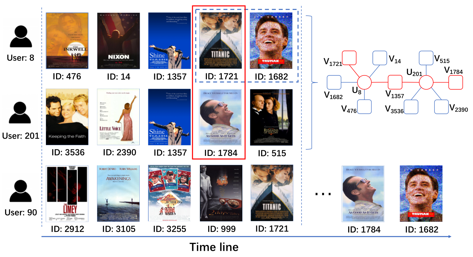
However, existing works for SR mainly put effort in modeling intra-sequence correlation yet neglect the effect of inter-sequence correlation. The authors in [\citeauthoryearHidasi et al.2016, \citeauthoryearQuadrana et al.2017, \citeauthoryearHidasi and Karatzoglou2018] apply recurrent neural networks (RNNs), which aggregate the sequence of the user’s interacted items to capture sequential correlation among the items. Different from RNN-based approaches, [\citeauthoryearTang and Wang2018, \citeauthoryearYuan et al.2019, \citeauthoryearXu et al.2019] treat the embedding matrix of items in a sequence as an image and apply convolutional neural networks (CNNs) to model sequential correlation. However, the above RNN-based and CNN-based approaches do not model the different impacts of the items consumed at different time steps on current decision. Hence, the authors in [\citeauthoryearKang and McAuley2018, \citeauthoryearSun et al.2019, \citeauthoryearZhang et al.2019] adopt attention networks to differentiate and learn the contribution of each individual item in a sequence to model the user interest when making predictions on next items. To obtain accurate item embedding and take complex transitions of items into account, Wu et al. [\citeauthoryearWu et al.2019] propose SR-GNN for session-based recommendation. In addition, gated networks [\citeauthoryearMa, Kang, and Liu2019] and neural variational models [\citeauthoryearXiao, Liang, and Meng2019] are also utilized in SR. However, the above mentioned methods mainly focus on modeling the intra-sequence item correlation within each individual sequence and the inter-sequence item correlation across different sequences is neglected. Though the intra-sequence item correlation is vital, we argue that explicitly modeling inter-sequence item correlation is also critical, as it not only captures the users’ general tastes, but also can help remedy the data scarce issue in SR[\citeauthoryearHe and McAuley2016].
To the best of our knowledge, only a few existing studies improve the recommendation quality by considering both intra- and inter-sequence item correlation in SR [\citeauthoryearRendle, Freudenthaler, and Schmidt-Thieme2010, \citeauthoryearHe and McAuley2016, \citeauthoryearWang et al.2019a]. FPMC [\citeauthoryearRendle, Freudenthaler, and Schmidt-Thieme2010] applies a first-order Markov Chain (MC) to model users’ sequential behavior and utilizes matrix factorization to learn the inter-sequence item correlation. Later, Fossil is proposed to address the data scarce problem by utilizing high-order Markov chain and similarity models [\citeauthoryearHe and McAuley2016]. Recently, Wang et al. propose Collaborative Session-based Recommendation Machine (CSRM) and consider inter-sequence correlation between different sessions. However, the inter-sequence information is not fully exploited in these works: (i) For FPMC and Fossil, the order of the inter-sequence item correlation is limited by the latent method, which is the MF and similarity model respectively; (ii) For CSRM, the inter-sequence correlation is considered in an implicit way, a simple session-level nearest neighbor-based approach.
Therefore, to make better use of inter-sequence item correlation, in this paper, we propose the Inter-Sequence enhanced framework for personalized Sequential Recommendation (ISSR), where both intra and inter-sequence item correlation are considered and encoded in two different modules. Figure 2 shows the workflow of the framework. In particular, inter-sequence item correlation is depicted with graphs. Graph neural networks are used to propagate the information along the paths between any two items. We choose graph neural network for its ability in modeling high-order item correlation and for its promising performance in information propagation [\citeauthoryearWang et al.2019b].
In summary, the main contributions are as follows:
- •
We propose the Inter-Sequence enhanced framework for personalized Sequential Recommendation (ISSR), which integrates both the intra-sequence and inter-sequence item correlation.
- •
In the inter-sequence item correlation encoder, graph neural networks are applied to encode high-order inter-sequence item correlation which is able to gather information from different sequences in an explicit manner.
- •
We conduct experimental studies on three real-world large-scale datasets. Extensive experimental results shows that 1) ISSR outperforms many state-of-the art models. 2) The performance of classic intra-sequence based models can be boosted significantly by adding up our proposed inter-sequence item correlation encoder. 3) The application of graph neural network in modeling inter-sequence correlation performs better than low-order, e.g. Matrix Factorization(MF)-based, methods.
Related Work
In this section, we review both the conventional and the deep learning-based methods for sequential recommendation.
Conventional methods. Two categories of conventional methods can be applied for sequential recommendation. The first category, such as Matrix Factorization [\citeauthoryearKoren, Bell, and Volinsky2009] and k-nearest neighbor [\citeauthoryearGuo et al.2019] methods, relies on computing user-item or item-item similarities for recommendation. However, this line of works ignore the sequential patterns in users’ behavior. In the second category, such as shani et al. [\citeauthoryearShani, Heckerman, and Brafman2005] tries to model item-item transitions in sequences with first-order Markov chains to capture the sequential patterns. And the authors in [\citeauthoryearRendle, Freudenthaler, and Schmidt-Thieme2010] considers both user-item similarities and first-order item-item transitions for sequential recommendation (FPMC). For better capturing user’s general interest and sequential patterns, Wang et al. [\citeauthoryearWang et al.2015] extend FPMC by using a hierarchical structure to learn uses representation. Moreover, he et al. [\citeauthoryearHe and McAuley2016] improve FPMC by utilizing high-order Markov chains to solve the sparsity problem in sequential recommendation. However, the above MC-based methods only model the intra-sequence interest between adjacent interactions.
Deep learning-based methods. Recently, benefit from the powerful feature representation ability, deep learning-based methods are increasingly popular in sequential recommendation. Recurrent Neural Network is the most popular technique for sequential recommendation [\citeauthoryearHidasi et al.2016, \citeauthoryearHidasi and Karatzoglou2018, \citeauthoryearRakkappan and Rajan2019], due to its inherent ability for modeling sequential dynamics. The authors in [\citeauthoryearHidasi et al.2016] utilize Gated Recurrent Units (GRU) to model the sequential dynamics for session-based recommendation, and use session-parallel mini-batches technique to train the model. What’s more, an improved version is proposed in [\citeauthoryearHidasi and Karatzoglou2018], where a novel ranking loss function and an efficient sampling strategy are proposed. In addition to the RNN-based methods, Convolutional Neural Network (CNN) is also adopted for sequential recommendation [\citeauthoryearTang and Wang2018, \citeauthoryearYuan et al.2019, \citeauthoryearXu et al.2019]. In [\citeauthoryearTang and Wang2018], the researchers embeds the recent engaged items into an “image” in the latent space, then employ different convolutional kernels to extract sequential patterns. And the authors in [\citeauthoryearYuan et al.2019] improves the work in [\citeauthoryearTang and Wang2018] by applying dilated convolutional layers and residual block structure such that the performance can be improved, especially for long sequences. Moreover, Xu et al. [\citeauthoryearXu et al.2019] combine RNN and CNN to learn user long- and short-term interest for sequential recommendation, where the hidden states of the RNN layer is the input the of the CNN layer. However, such RNN- and CNN-based methods always encodes the user interactions into hidden states or latent factors without considering the different impacts of the items consumed at different time steps on current decision. Therefore, the attention based models, which exhibit promising performance in sequence learning, are also utilized in sequential recommendation[\citeauthoryearKang and McAuley2018, \citeauthoryearSun et al.2019]. In addition, the authors in [\citeauthoryearMa, Kang, and Liu2019] propose to utilize gated network for sequential recommendation, where a feature gating layer and an instance gating layer are employed to select what item features can be passed to the downstream layers from the feature and instance levels, respectively. Recently, Graph Neural Networks (GNN) gains great attentions in recommendation community [\citeauthoryearPerozzi, Al-Rfou, and Skiena2014, \citeauthoryearTang et al.2015, \citeauthoryearGrover and Leskovec2016, \citeauthoryearZhou et al.2017, \citeauthoryearWu et al.2019], and the authors in [\citeauthoryearWu et al.2019] firstly employ GNN for session based recommendation. It models the sequences of items for each sessions separately, however, the ability of capturing the cross-sequence interest among the items is limited. Moreover, in other lines of work, transfer learning [\citeauthoryearMa et al.2019] and variational model [\citeauthoryearXiao, Liang, and Meng2019] are also utilized for sequential recommendation.
As we can see, the majority of the conventional and deep learning-based methods for sequential recommendation focus on intra-sequence interest within each individual sequence, but neglect the inter-sequence interest across different sequences. Different from above methods, our proposed MGSR coordinates the intra-sequence interest and inter-sequence interest modeling in sequential recommendation.
Problem Formulation
Let and denote the set of users and the set of items, respectively. Given the sequences of interacted items from all users, the goal of sequential recommendation is to recommend a list of items from to each user such that the user is most likely to interact with the recommended items. For a specific user, our framework outputs the probabilities for all candidate items, which represent how likely she will engage with the items based on her engaged sequence of items.
Methodology
As shown in Figure 2, the proposed framework ISSR consists of an inter-sequence item correlation encoder, an intra-sequence item correlation encoder, and a prediction decoder. Firstly, we model the inter-sequence item correlation with two graphs, which are the user-item bipartite graph [\citeauthoryearWang et al.2019b] and the item-item co-occurrence graph [\citeauthoryearLi et al.2019]. Based on these graphs, the high-order inter-sequence item correlation can be captured through stacking multiple GNN layers. Although the bipartite graph and co-occurrence graph have already been utilized in recommender systems, we are the first to combine the two graphs to exploit the high-order inter-sequence item correlation in sequential recommendation scenario. Next, an intra-sequence item correlation encoder is developed, which pre-fuse the inter-sequence item correlation information with their intra-sequence sequential correlation and temporal dynamics. And we then integrate the item representations, which comprehensively captures both the inter- and intra-sequence item correlation, to generate the representation of the user’s current interest. Finally, in the prediction decoder, the user’s preference on different items is computed based on the user’s interest representation. Each part will be elaborated in the following.


Inter-sequence Item Correlation Encoder
To obtain the informative inter-sequence item correlation, we propose an item correlation encoder, which is specified in Figure 3. As Figure 3 shows, ISSR exploits the item correlation from both the user-item bipartite graph and the item-item co-occurrence graph. In addition, ISSR also considers the residual connection to preserve the original item representation. Finally, we generate the integrated item representation by fusing the three types of item information.
Inter-sequence Item Correlation from User-Item Bipartite Graph.
The user-item bipartite graph contains two types of nodes, namely the user nodes and the item nodes. An edge exists between a user and an item if the user interacted with the item. For clarity, the adjacent nodes of a target node in the graph is defined as the -hop neighbors of the target node. Particularly, for each node in the graph, denotes the set of 1-hop neighbors of . Thus, the high-order inter-sequence item correlation can be seized via multiple hops on the graph through the user nodes. For easy to follow, a path connected with multiple item nodes and user nodes is highlighted in the bipartite graph (the top left of Figure 3), where the correlation between item nodes located in the start and the end of the path can be captured22 2 Note that the arrows only highlight the paths, and the two graphs are undirected.. We apply graph convolutional network [\citeauthoryearYing et al.2018] on the user-item bipartite graph (denoted as GCNB) to aggregate the neighborhood information. As a result, the item correlation from the -hop neighbors can be captured via stacking multiple GCN layers.
We denote the initial embedding of item node as with dimension (or for the user node ) and the hidden representation of at layer- as (or as for the user node ). In GCNB, a node embedding depends on both the node information and the graph structure around it. We first aggregate the neighborhood information of the target node (as shown in Eq. (1)), and then integrate the aggregated neighborhood information with the target node (as shown in Eq. (2)).
Specifically, we represent the neighborhood of an item node at layer- (or a user node at layer-), by applying an aggregate function on all its neighbors at layer-(-):
| (1) |
(or ) is the representation of the neighborhood of item node (or of user node ) at layer-(-). and (or, and ) are the weight matrix and bias of the item (or user) aggregator at layer-, respectively. A pooling function (such as weighted sum, weighted average, and etc.) is performed to aggregate the neighbor representations. is an activation function.
Note that different neural networks are utilized to transform the representations of the user nodes and item nodes from lower layers to higher layers, which differs form existing GCN works [\citeauthoryearYing et al.2018, \citeauthoryearWang et al.2019b], where normally a unified network is utilized. The reason is that user nodes and item nodes in bipartite graphs are intrinsically different and such difference should be considered when we aggregate information from user nodes or from item nodes.
After generalizing the representation of the target node’s neighborhood, we integrate such neighborhood representation with the current representation of the target node, as:
| (2) | ||||
and (or, and ) are the transformation weight matrix and bias of the item (or user) at layer-, respectively. represents concatenation.
Inter-sequence Item Correlation from Item-Item Co-occurrence Graph
The GCNB captures the item correlation through multiple-hop neighbors in the user-item bipartite graph. In addition, the item correlation can also be modeled from an item-item graph. Though there exists multiple methods to construct such an item-item graph. We utilize item co-occurrence information in users’ behavior sequences to build it following [\citeauthoryearLi et al.2019], which can be treated as a complementary of the user-item bipartite graph to directly model the frequency of item dependence.
As shown in Figure 3, the co-occurrence graph includes a set of nodes where each node represents an item. An edge connects two nodes, if these two items are adjacent in a certain user’s behavior sequence. The weight of an edge represents the number of times that the two items occur in users’ behavior sequences, and such weight is utilized for neighborhood sampling, which we specify it later. We apply the graph convolutional network on such item-item co-occurrence graph where we denote it as GCNC. GCNC works differently from GCNB in the following two aspects. First, the item-item co-occurrence graph includes only one type of nodes, so that GCNC has neither aggregator weight matrices nor transformation weight matrices for user nodes. Second, the item-item co-occurrence graph associates weights on edges, which results in a different neighborhood sampling strategy as we will discuss in ‘Network Training’ section. Due to the limit of space, we will not elaborate the details of GCNC. We represent the embedding of an item node in this item-item co-occurrence graph as .
In summary, the user-item bipartite graph and the item-item co-occurrence graph are designed to capture the inter-sequence item correlation, which act as complementary roles.
Residual Connection
Inspired by [\citeauthoryearKang and McAuley2018], we introduce the residual connection component in the inter-sequence item correlation encoder, which plays a role of preserving the original item representations: . where is the original embedding of the item . The residual connection transforms the original embedding to via a hidden layer with and .
Information Fusion
As presented in Figure 3, the item representations learned from the two graphs and the residual connection are fused through an information fusion function . More formally, the final representation of an item is generated as: , and varies according to different application scenarios. In this paper, we empirically choose element-wise sum as the fusion function (sum pooling in Figure 3) due to its superior performance compared to the other operations, such as concatenation and element-wise mean and gated networks [\citeauthoryearDauphin et al.2017].
Intra-sequence Item Correlation Encoder
In the intra-sequence item correlation encoder, ISSR aims to model the intra-sequence item correlation with considering the inter-sequence item correlation captured in the inter-sequence item correlation encoder, and finally integrate the user’s current interest over the candidate items. As presented in Figure 2, a GRU layer is performed to capture the intra-sequence item sequential correlation among the items in a sequence, where the hidden states in the GRU layer represent user’s interests at different time steps. Then an attention network is utilized to aggregate the user’s interests at different time steps, generating the final representation of the user’s current interest.
The GRU Layer
As shown in Figure 2, the input of the GRU layer is a sequence of items, of which the embeddings are learned from the inter-sequence item correlation encoder. The GRU layer outputs a sequence of hidden vectors , which represent the user’s interests at different time steps.
The Attention Layer
User’s interests at different time steps contribute differently to the user’s current decision. Moreover, different users have different levels of sensitivity to the temporal dynamics. Due to such motivations, we devise a personalized attention network to capture the evolving interests of each particular user.
Specifically, the inputs of the attention network are the sequence of hidden states generated by the GRU layer, e.g., , and the embedding of the user . With multi-layer perceptrons, the attention network generates a weight for each input hidden state representing the contribution of the user’s interest at that time step (represented by the input hidden vector) on the user’s final decision.
| (3) |
As shown in Eq. (3), is the weight of the hidden state on the final decision of user . are parameters of the multi-layer perceptrons. For simplicity, we only present two layers of parameters in multi-layer perceptions in Eq. (3), which is also the case in our implementation. The user’s interest, considering both the intra-sequence item sequential correlation and the temporal dynamics, is computed as:
| (4) |
As shown in [\citeauthoryearWu et al.2019], the latest engaged item is able to reflect user’s most recent interest. Therefore, we integrate the latest hidden state into user’s final interest representation:
Prediction Decoder
After obtaining the representation of the user’s current interest, we adopt the classic matrix factorization approach to infer the user’s preference on the items. The prediction score of user on item is the inner product of the user’s interest and the item embedding . The probability that the user will interact with the item is defined as the softmax of the prediction score: .
Network Training
Loss Function
To generate the training data, we extract consecutive items in a sequence as user’s behavior sequence and the following items as positive samples. We also sample a number of items that the user did not interacted with as negative samples following [\citeauthoryearKang and McAuley2018]. We adopt cross entropy as the training loss to describe the discrepancy between the predicted probabilities and the ground truth labels as shown in Eq. (5) .
| (5) |
where is the number of instances, if the predicted item is engaged by the user; otherwise, .
Neighborhood Sampling
We adopt neighborhood sampling techniques to facilitate the network training. Specifically, for GCNB on the bipartite graph, we sample neighbors for each node uniformly at random. For GCNC on the co-occurrence graph, we apply importance sampling, which samples neighbors for each node according to the weights of the edges.
Experiments
In this section, we compare the proposed framework with the state-of-the-art methods on three real-world datasets. We also comprehensively analyze the results of the proposed framework under different experimental settings.
Datasets
Experiments are conducted on the following three public benchmark datasets: MovieLens (1M) (abbreviated as ML (1M)), Steam [\citeauthoryearKang and McAuley2018], MovieLens (20M) (abbreviated as ML (20M)), which is of different scales and sparsity. We process the three datasets following the existing research [\citeauthoryearTang and Wang2018], in which all the ratings are treated as implicit feedbacks. And the items in a user’s sequence are sorted in chronological order. We hold the first 70%, following 10% and last 20% of items in each user’s sequence as the training set, the validation set and the testing set, respectively33 3 Note that the data partition strategy is different from the original SASRec [\citeauthoryearKang and McAuley2018], they treat the last item in the whole sequence of each user as the test set, the second last item as validation set, and all the previous items as training set. So their training set is much larger than the one utilized in this paper while the test set is much smaller. Moreover, in HGN, the authors treat all the ratings less than four as negative samples, and then filter the noise data. However, in Caser, the authors treat all the ratings as implicit feedbacks. Therefore, the size of the ML (20) dataset in HGN is only half of that in this paper.. The statistics of the three processed datasets are summarized in Table 1.
| Datasets | #users | #items | avg.#items/user | sparsity | #interactions |
|---|---|---|---|---|---|
| ML (1M) | 6,040 | 3,416 | 165.50 | 95.16% | 999,611 |
| Steam | 334,730 | 13,047 | 11.01 | 99.92% | 3,686,172 |
| ML (20M) | 138,493 | 15,451 | 144.16 | 99.07% | 19,964,833 |
Experimental Settings
Evaluation Metrics
Following [\citeauthoryearTang and Wang2018], we adopt Recall@, nDCG@, HR@ and MRR@ for to evaluate the effectiveness of different methods.
Compared Methods
To demonstrate the superiority of the proposed ISSR, we compare it to several state-of-the-art baselines. For easy to follow, we summarize them into two categories according to whether they can model the inter- and intra-sequence item correlation, namely (1) only intra-sequence based methods: GRU4Rec [\citeauthoryearHidasi et al.2016], Caser [\citeauthoryearTang and Wang2018], SASRec [\citeauthoryearKang and McAuley2018], SR-GNN [\citeauthoryearWu et al.2019] and HGN [\citeauthoryearMa, Kang, and Liu2019]; (2) both inter- and intra-sequence based methods: FPMC [\citeauthoryearRendle, Freudenthaler, and Schmidt-Thieme2010], Fossil [\citeauthoryearHe and McAuley2016] and CSRM [\citeauthoryearWang et al.2019a].
Methods such as the popularity [\citeauthoryearCremonesi, Koren, and Turrin2010] and BPR-MF [\citeauthoryearRendle et al.2009] which we treat as only inter-sequence based methods are omitted in comparison, because they are proven to be inferior to the compared methods as they lack the ability of modeling intra-sequence sequential correlation [\citeauthoryearTang and Wang2018, \citeauthoryearMa, Kang, and Liu2019].
We implement FPMC, Fossil and ISSR using TensorFlow with Adam [\citeauthoryearKingma and Ba2014] optimizer. We utilize the source code of GRU4Rec, Caser, SASRec, SR-GNN, CSRM, HGN to re-produce their performance.
| Dataset | Model | Recall@5 | Recall@10 | nDCG@5 | nDCG@10 | HR@5 | HR@10 | MRR@5 | MRR@10 | |
|---|---|---|---|---|---|---|---|---|---|---|
| ML (1M) | Intra | GRU4Rec | 0.0707 | 0.1232 | 0.4661 | 0.5012 | 0.1558 | 0.2507 | 0.0792 | 0.0918 |
| Caser | 0.0764 | 0.1326 | 0.4783 | 0.5176 | 0.1613 | 0.2624 | 0.0826 | 0.0961 | ||
| SASRec | 0.0812 | 0.1320 | 0.4778 | 0.5156 | 0.1726 | 0.2773 | 0.0891 | 0.1018 | ||
| SR-GNN | 0.0834 | 0.1385 | 0.4859 | 0.5234 | 0.1854 | 0.2906 | 0.1034 | 0.1152 | ||
| HGN | 0.0816 | 0.1378 | 0.4973 | 0.5295 | 0.1836 | 0.2945 | 0.1012 | 0.1154 | ||
| intra | FPMC | 0.0653 | 0.1095 | 0.4183 | 0.4632 | 0.1567 | 0.2554 | 0.0798 | 0.0904 | |
| and | Fossil | 0.0701 | 0.1213 | 0.4555 | 0.4925 | 0.1611 | 0.2501 | 0.0803 | 0.0912 | |
| inter | CSRM | 0.0815 | 0.1381 | 0.4901 | 0.5238 | 0.1768 | 0.2836 | 0.0965 | 0.1107 | |
| ISSR | ||||||||||
| Improv. | 11.99% | 12.85% | 7.66% | 6.36% | 16.34% | 12.67% | 14.70% | 15.86% | ||
| Steam | Intra | GRU4Rec | 0.0381 | 0.0714 | 0.0485 | 0.0702 | 0.0404 | 0.0755 | 0.0134 | 0.0181 |
| Caser | 0.0408 | 0.0744 | 0.0507 | 0.0735 | 0.0459 | 0.0825 | 0.0158 | 0.0206 | ||
| SASRec | 0.0403 | 0.0737 | 0.0502 | 0.0726 | 0.0447 | 0.0821 | 0.0151 | 0.0199 | ||
| SR-GNN | 0.0415 | 0.0759 | 0.0548 | 0.0782 | 0.0472 | 0.0837 | 0.0181 | 0.0232 | ||
| HGN | 0.0437 | 0.0767 | 0.0588 | 0.0803 | 0.0495 | 0.0851 | 0.0200 | 0.0247 | ||
| intra | FPMC | 0.0354 | 0.0612 | 0.0491 | 0.0663 | 0.0380 | 0.0658 | 0.0174 | 0.0210 | |
| and | Fossil | 0.0408 | 0.0745 | 0.0504 | 0.0721 | 0.0455 | 0.0800 | 0.0171 | 0.0232 | |
| inter | CSRM | 0.0427 | 0.0747 | 0.0573 | 0.0773 | 0.0453 | 0.0825 | 0.0197 | 0.0239 | |
| ISSR | ||||||||||
| Improv. | 12.59% | 13.69% | 9.52% | 10.09% | 11.31% | 14.22% | 11.94% | 12.15% | ||
| ML (20M) | Intra | GRU4Rec | 0.0584 | 0.1031 | 0.3171 | 0.3612 | 0.0963 | 0.1630 | 0.0477 | 0.0564 |
| Caser | 0.0644 | 0.1127 | 0.3371 | 0.3829 | 0.1045 | 0.1750 | 0.0530 | 0.0623 | ||
| SASRec | 0.0624 | 0.1102 | 0.3341 | 0.3794 | 0.1177 | 0.1940 | 0.0609 | 0.0756 | ||
| SR-GNN | 0.0752 | 0.1271 | 0.3643 | 0.4060 | 0.1349 | 0.2142 | 0.0710 | 0.0814 | ||
| HGN | 0.0812 | 0.1350 | 0.3749 | 0.4135 | 0.1468 | 0.2288 | 0.0780 | 0.0888 | ||
| intra | FPMC | 0.0569 | 0.0982 | 0.3054 | 0.3459 | 0.0928 | 0.1515 | 0.0476 | 0.0548 | |
| and | Fossil | 0.0607 | 0.1030 | 0.3152 | 0.3681 | 0.0989 | 0.1589 | 0.0483 | 0.0562 | |
| inter | CSRM | 0.0724 | 0.1259 | 0.3625 | 0.4054 | 0.1370 | 0.2102 | 0.0650 | 0.0759 | |
| ISSR | ||||||||||
| Improv. | 8.74% | 10.00% | 8.64% | 7.67% | 10.29% | 12.28% | 8.72% | 9.57% | ||
Parameter Settings
The best hyper-parameters for each model are found from exhaustive search on the validation set. In particular, for Caser, the number of the vertical and horizontal filters are searched from . For SASRec, the number of self-attention blocks is searched from . For SR-GNN and HGN, we follow the best parameter settings in the original paper. For CSRM, the memory size is searched from for different dataset. For our proposed framework ISSR, the neighborhood information is aggregated from at most 3-hop due to the efficiency concern. The best performance is observed when we consider 2-hop neighbors in GCNB and 1-hop neighbors in GCNC. We follow the settings in [\citeauthoryearTang and Wang2018, \citeauthoryearMa, Kang, and Liu2019] to set the sequence length to be 5 (i.e., ) and the number of subsequent items to be 3 (i.e., ) for all methods, unless stated otherwise, for fair comparison.
Overall Performance Comparison
Table 2 summarizes the overall performance of all the compared models on the three datasets, where the underlined numbers are the best results of the baselines, and the bold numbers are the best results of all models. indicates the statistically significant improvement [\citeauthoryearRuxton2006] (i.e., two-sided t-test) with p-value over the best baselines. The row “%Improv.” indicates the relative improvement of ISSR compared to the best baselines. We have the following observations.
ISSR is more superior than HGN, SR-GNN, SASRec, Caser and GRU4Rec. This is due to three possible reasons. First, except for capturing the intra-sequence item correlation with GRU and attention layers, the two graphs constructed by ISSR capture the inter-sequence item correlation across different users. Differently, no matter how the session graph is constructed by SR-GNN or the other methodology utilized in baselines, they only consider the intra-sequence item correlation within each individual session. Second, residual connections in ISSR preserve the original item representations, served as a complementary to the item representations produced by the graph neural network, which makes the item representations more informative. Third, the attention network in ISSR is personalized based on the fact that users may have different levels of sensitivity to temporal dynamics, which is not considered by the baseline methods.
ISSR outperforms FPMC, Fossil and CSRM, the reasons are as follows: (1) for FPMC and Fossil, ISSR captures high-order inter-sequence item correlation from the two graph neural networks with multiple hops, whereas, FPMC and Fossil only capture low-order inter-sequence item correlation with MF and similarity based model; In addition, FPMC and Fossil both utilize Markov Chains to model the intra-sequence item sequential correlation, which is proven to be inferior to deep neural network based model [\citeauthoryearHidasi et al.2016, \citeauthoryearTang and Wang2018, \citeauthoryearKang and McAuley2018]; (2) for CSRM, it captures inter-sequence correlation with a simple session-level nearest neighbor-based approach instead of the fine-grained item-level correlation we addressed in ISSR.
Another observation is that, on the sparse Steam dataset, Fossil achieves comparable performance to Caser and SASRec, or even slightly better w.r.t. Recall@10 etc. evaluation metrics. This observation also indicates that explicitly modeling the inter-sequence item correlation can remedy the data scarce issue to some extent.
To summarize, ISSR shows consistent and significant improvement over the compared baselines on all the (dense or sparse, small or large scale) conducted datasets in terms of Recall, nDCG, HR and MRR, which demonstrates the superiority of our proposed framework.
Effect of Inter-sequence Item Correlation Encoder for Sequential Recommendation
To verify the effectiveness of the proposed inter-sequence item correlation encoder, we incorporate the proposed inter-sequence item correlation encoder into the existing RNN-based, CNN-based and attention-based sequential recommendation methods, respectively. The results are reported in Table 3. From Table 3, we observe that these models are enhanced after equipping the proposed inter-sequence item correlation encoder. For instance, we achieve 25.0%, 14.8% and 9.0% improvements in terms of Recall@10 on MovieLens (1M) datasets. The observation demonstrates that modeling the inter-sequence item correlation as in the proposed ISSR can boost the performance of existing SR methods.
| variants | ML(1M) | Steam | ||
|---|---|---|---|---|
| Recall@10 | nDCG@10 | Recall@10 | nDCG@10 | |
| GRU4Rec | 0.1232 | 0.5012 | 0.0714 | 0.0702 |
| Inter+GRU4Rec | 0.1545 | 0.5609 | 0.0856 | 0.0872 |
| SASRec | 0.1320 | 0.5156 | 0.0737 | 0.0726 |
| Inter+SASRec | 0.1558 | 0.5621 | 0.0864 | 0.0878 |
| Caser | 0.1326 | 0.5176 | 0.0744 | 0.0735 |
| Inter+Caser | 0.1445 | 0.5460 | 0.0815 | 0.0828 |
Effect of the Graphs in Inter-Sequence Item Correlation Encoder
To verify the effectiveness of the bipartite and the co-occurrence graphs in capturing high-order inter-sequence item correlations, we design several variants of the inter-sequence encoder. These variants are Only intra, MF+intra, Co+intra, Bi+intra and ISSR as shown in Tables 4 where ISSR is our proposed framework. They represent null, MF-based low order, co-occurrence graph based high order, bipartite graph based high order and dual graph based high order inter-sequence encoder, respectively. From Table 4, we have the following observations. (1) Only intra performs obviously worse than the other variants which demonstrates the indispensability of the inter-sequence encoder. (2) The performance of MF+intra is inferior to the graph based inter-sequence encoder due to MF’s inability in explicitly capturing higher order item correlations across different sequences. Graph neural networks can model the high-order item correlations across different sequences with multiple hops. (3) The minor difference observed between Bi+intra and Co+intra indicates user-item bipartite graph and item-item co-occurrence graph contribute almost equally to the final performance, and combining the two graphs together will enhance the performance.
| variants | ML(1M) | Steam | ||
|---|---|---|---|---|
| Recall@10 | nDCG@10 | Recall@10 | nDCG@10 | |
| Only intra | 0.1378 | 0.5244 | 0.0747 | 0.0772 |
| MF+intra | 0.1412 | 0.5265 | 0.0766 | 0.0787 |
| Co+intra | 0.1541 | 0.5604 | 0.0852 | 0.0865 |
| Bi+intra | 0.1548 | 0.5608 | 0.0856 | 0.0869 |
| ISSR | 0.1563 | 0.5632 | 0.0872 | 0.0884 |
Effect of Dimensionality of Item Embedding
Figure 4 presents the performance of all the compared models varying the dimension of item embedding. Due to the space limit, we only present the Recall@10 on ML(1M) and Steam. As we increase , the performance of all the models increases until reaching the best values. Then, the performance drops or keeps stable as we continue increasing . The reason is that the capacity of the models increases as the dimensionality of item embeddings is enlarged. However, after reaching its peak value, the model capacity will not keep increasing even if the dimensionality of item embeddings continues increasing since the model capacity is limited by the amount of informative data. ISSR reaches its best performance when setting .

Conclusion
In this paper, we propose a Inter-Sequence enhanced framework for personalized Sequential Recommendation (ISSR). The inter-sequence item correlation encoder in ISSR utilizes two graphs (i.e., a user-item bipartite graph and an item-item co-occurrence graph) to capture the inter-sequence item correlations. The intra-sequence item correlation encoder aggregates the learned inter-sequence item correlation information and considers the item sequential correlations and temporal dynamics in a current sequence to generate the representation of users’ interests. Then the user’s next behavior on the candidate items can be predicted by the learned interests. Extensive experiments on three real-world datasets are conducted. The results demonstrate the superiority of ISSR over many state-of-the-art methods.
References
- [\citeauthoryearCremonesi, Koren, and Turrin2010] Cremonesi, P.; Koren, Y.; and Turrin, R. 2010. Performance of recommender algorithms on top-n recommendation tasks. In Proceedings of the fourth ACM conference on Recommender systems, RecSys, 39–46. ACM.
- [\citeauthoryearDauphin et al.2017] Dauphin, Y. N.; Fan, A.; Auli, M.; and Grangier, D. 2017. Language modeling with gated convolutional networks. In ICML, 933–941. JMLR. org.
- [\citeauthoryearGrover and Leskovec2016] Grover, A., and Leskovec, J. 2016. node2vec: Scalable feature learning for networks. In Proceedings of the 22nd ACM SIGKDD international conference on Knowledge discovery and data mining, 855–864. ACM.
- [\citeauthoryearGuo et al.2019] Guo, H.; Tang, R.; Ye, Y.; Liu, F.; and Zhang, Y. 2019. A novel KNN approach for session-based recommendation. In PAKDD, 381–393.
- [\citeauthoryearHe and McAuley2016] He, R., and McAuley, J. 2016. Fusing similarity models with markov chains for sparse sequential recommendation. In ICDM, 191–200. IEEE.
- [\citeauthoryearHidasi and Karatzoglou2018] Hidasi, B., and Karatzoglou, A. 2018. Recurrent neural networks with top-k gains for session-based recommendations. In CIKM, 843–852. ACM.
- [\citeauthoryearHidasi et al.2016] Hidasi, B.; Karatzoglou, A.; Baltrunas, L.; and Tikk, D. 2016. Session-based recommendations with recurrent neural networks. In 4th International Conference on Learning Representations, ICLR 2016, San Juan, Puerto Rico, May 2-4, 2016, Conference Track Proceedings.
- [\citeauthoryearKang and McAuley2018] Kang, W., and McAuley, J. J. 2018. Self-attentive sequential recommendation. In IEEE International Conference on Data Mining, ICDM 2018, Singapore, November 17-20, 2018, 197–206.
- [\citeauthoryearKingma and Ba2014] Kingma, D. P., and Ba, J. 2014. Adam: A method for stochastic optimization. arXiv preprint arXiv:1412.6980.
- [\citeauthoryearKoren, Bell, and Volinsky2009] Koren, Y.; Bell, R.; and Volinsky, C. 2009. Matrix factorization techniques for recommender systems. Computer (8):30–37.
- [\citeauthoryearLi et al.2019] Li, F.; Chen, Z.; Wang, P.; Ren, Y.; Zhang, D.; and Zhu, X. 2019. Graph intention network for click-through rate prediction in sponsored search. In SIGIR, 961–964. ACM.
- [\citeauthoryearMa et al.2019] Ma, M.; Ren, P.; Lin, Y.; Chen, Z.; Ma, J.; and de Rijke, M. 2019. -net: A parallel information-sharing network for shared-account cross-domain sequential recommendations. In Proceedings of the 42nd International ACM SIGIR Conference on Research and Development in Information Retrieval, SIGIR 2019, Paris, France, July 21-25, 2019, 685–694.
- [\citeauthoryearMa, Kang, and Liu2019] Ma, C.; Kang, P.; and Liu, X. 2019. Hierarchical gating networks for sequential recommendation. In KDD 2019, Anchorage, AK, USA, August 4-8, 2019, 825–833.
- [\citeauthoryearPerozzi, Al-Rfou, and Skiena2014] Perozzi, B.; Al-Rfou, R.; and Skiena, S. 2014. Deepwalk: Online learning of social representations. In Proceedings of the 20th ACM SIGKDD international conference on Knowledge discovery and data mining, 701–710. ACM.
- [\citeauthoryearQuadrana et al.2017] Quadrana, M.; Karatzoglou, A.; Hidasi, B.; and Cremonesi, P. 2017. Personalizing session-based recommendations with hierarchical recurrent neural networks. In Proceedings of the Eleventh ACM Conference on Recommender Systems, RecSys 2017, Como, Italy, August 27-31, 2017, 130–137.
- [\citeauthoryearRakkappan and Rajan2019] Rakkappan, L., and Rajan, V. 2019. Context-aware sequential recommendations withstacked recurrent neural networks. In WWW 2019, San Francisco, CA, USA, May 13-17, 2019, 3172–3178.
- [\citeauthoryearRendle et al.2009] Rendle, S.; Freudenthaler, C.; Gantner, Z.; and Schmidt-Thieme, L. 2009. Bpr: Bayesian personalized ranking from implicit feedback. In Proceedings of the twenty-fifth conference on uncertainty in artificial intelligence, 452–461. AUAI Press.
- [\citeauthoryearRendle, Freudenthaler, and Schmidt-Thieme2010] Rendle, S.; Freudenthaler, C.; and Schmidt-Thieme, L. 2010. Factorizing personalized markov chains for next-basket recommendation. In WWW 2010, Raleigh, North Carolina, USA, April 26-30, 2010, 811–820.
- [\citeauthoryearRuxton2006] Ruxton, G. D. 2006. The unequal variance t-test is an underused alternative to student’s t-test and the mann–whitney u test. Behavioral Ecology 17(4):688–690.
- [\citeauthoryearShani, Heckerman, and Brafman2005] Shani, G.; Heckerman, D.; and Brafman, R. I. 2005. An mdp-based recommender system. Journal of Machine Learning Research 6(Sep):1265–1295.
- [\citeauthoryearSun et al.2019] Sun, F.; Liu, J.; Wu, J.; Pei, C.; Lin, X.; Ou, W.; and Jiang, P. 2019. Bert4rec: Sequential recommendation with bidirectional encoder representations from transformer. arXiv preprint arXiv:1904.06690.
- [\citeauthoryearTang and Wang2018] Tang, J., and Wang, K. 2018. Personalized top-n sequential recommendation via convolutional sequence embedding. In Proceedings of the Eleventh ACM International Conference on Web Search and Data Mining, WSDM ’18, 565–573. New York, NY, USA: ACM.
- [\citeauthoryearTang et al.2015] Tang, J.; Qu, M.; Wang, M.; Zhang, M.; Yan, J.; and Mei, Q. 2015. Line: Large-scale information network embedding. In Proceedings of the 24th international conference on world wide web, WWW, 1067–1077. International World Wide Web Conferences Steering Committee.
- [\citeauthoryearWang et al.2015] Wang, P.; Guo, J.; Lan, Y.; Xu, J.; Wan, S.; and Cheng, X. 2015. Learning hierarchical representation model for nextbasket recommendation. In SIGIR, 403–412. ACM.
- [\citeauthoryearWang et al.2019a] Wang, M.; Ren, P.; Mei, L.; Chen, Z.; Ma, J.; and de Rijke, M. 2019a. A collaborative session-based recommendation approach with parallel memory modules. In SIGIR , Paris, France, July 21-25, 2019, 345–354.
- [\citeauthoryearWang et al.2019b] Wang, X.; He, X.; Wang, M.; Feng, F.; and Chua, T.-S. 2019b. Neural graph collaborative filtering. In SIGIR.
- [\citeauthoryearWu et al.2019] Wu, S.; Tang, Y.; Zhu, Y.; Wang, L.; Xie, X.; and Tan, T. 2019. Session-based recommendation with graph neural networks. In The Thirty-Third AAAI Conference on Artificial Intelligence, 346–353.
- [\citeauthoryearXiao, Liang, and Meng2019] Xiao, T.; Liang, S.; and Meng, Z. 2019. Hierarchical neural variational model for personalized sequential recommendation. In WWW 2019, San Francisco, CA, USA, May 13-17, 2019, 3377–3383.
- [\citeauthoryearXu et al.2019] Xu, C.; Zhao, P.; Liu, Y.; Xu, J.; S Sheng, V. S. S.; Cui, Z.; Zhou, X.; and Xiong, H. 2019. Recurrent convolutional neural network for sequential recommendation. In WWW, 3398–3404. ACM.
- [\citeauthoryearYing et al.2018] Ying, R.; He, R.; Chen, K.; Eksombatchai, P.; Hamilton, W. L.; and Leskovec, J. 2018. Graph convolutional neural networks for web-scale recommender systems. In Proceedings of the 24th ACM SIGKDD International Conference on Knowledge Discovery & Data Mining, 974–983.
- [\citeauthoryearYuan et al.2019] Yuan, F.; Karatzoglou, A.; Arapakis, I.; Jose, J. M.; and He, X. 2019. A simple convolutional generative network for next item recommendation. In Proceedings of the Twelfth ACM International Conference on Web Search and Data Mining, WSDM 2019, Melbourne, VIC, Australia, February 11-15, 2019, 582–590.
- [\citeauthoryearZhang et al.2019] Zhang, S.; Tay, Y.; Yao, L.; Sun, A.; and An, J. 2019. Next item recommendation with self-attentive metric learning. In Thirty-Third AAAI Conference on Artificial Intelligence, volume 9.
- [\citeauthoryearZhou et al.2017] Zhou, C.; Liu, Y.; Liu, X.; Liu, Z.; and Gao, J. 2017. Scalable graph embedding for asymmetric proximity. In Thirty-First AAAI Conference on Artificial Intelligence, AAAI.