跳到论文正文
W Papers独立论文阅读器 arXiv:2004.11926 论文正文 计算阅读时间 · 0%
引用这篇论文根据当前论文元数据生成,正式投稿前建议核对。


License: arXiv.org perpetual non-exclusive license
arXiv:2004.11926v1 [math.AT] 24 Apr 2020

Local Equivalence of Metrics for Multiparameter Persistence Modules

Oliver Vipond Affiliation: vipond@maths.ox.ac.uk University of Oxford, Andrew Wiles Building, Woodstock Rd, Oxford OX2 6GG
Abstract

An ideal invariant for multiparameter persistence would be discriminative, computable and stable. In this work we analyse the discriminative power of a stable, computable invariant of multiparameter persistence modules: the fibered bar code. The fibered bar code is equivalent to the rank invariant and encodes the bar codes of the 1-parameter submodules of a multiparameter module. This invariant is well known to be globally incomplete. However in this work we show that the fibered bar code is locally complete for finitely presented modules by showing a local equivalence of metrics between the interleaving distance (which is complete on finitely-presented modules) and the matching distance on fibered bar codes. More precisely, we show that: for a finitely-presented multiparameter module MM there is a neighbourhood of MM, in the interleaving distance dId_{I}, for which the matching distance, d0d_{0}, satisfies the following bi-Lipschitz inequalities 134​dI​(M,N)≤d0​(M,N)≤dI​(M,N)\frac{1}{34}d_{I}(M,N)\leq d_{0}(M,N)\leq d_{I}(M,N) for all NN in this neighbourhood about MM. As a consequence no other module in this neighbourhood has the same fibered bar code as MM.

1 Introduction

The theory and application of multiparameter persistent homology is a topic of significant interest in the field of Topological Data Analysis. Current work has studied invariants and metrics of multiparameter persistence modules, together with algorithms for their efficient computation [Vip18, KLO19, DX19, LW19].

Compared to single parameter persistence, studying data sets filtered over multiple parameters yields a richer class of topological invariants: multiparameter persistence modules. A distinct difference between multiparameter and single parameter persistence modules is that multiparameter modules do not admit a discrete complete invariant analogous to the bar code for single parameter persistence modules [CZ09]. Another upshot of the increased complexity of multiparameter modules, is that the analogous interleaving distance cannot be reduced to a matching distance as in the single parameter case and is thus harder to compute [BBK19].

An ideal invariant for multiparameter persistence would be discriminative, computable and stable. In earlier work studying invariants for multiparameter persistence, it is common to sacrifice the discriminating power of an invariant in order to achieve computability [Vip18, MP19, Cor+19]. Also it is common to study subclasses of persistence modules to tame the wild behaviour of arbitrary multiparameter modules. Such subclasses include: exact [CO20], interval decomposable [Bje16, DX19], block decomposable [BL18, CO20, BBK19] and rectangular interval decomposable [BLO20] multiparameter persistence modules. For data science applications, stability is an essential property of a multiparameter module invariant; indeed most data is susceptible to noise and so we desire that our invariants be robust to small perturbations.

A discriminative, stable metric one could choose to study multiparameter persistence modules is the interleaving distance [Les15]. The theoretical properties of the interleaving distance are well-behaved. Lesnick showed that the interleaving distance is universal on the space of multiparameter modules, and thus the most discriminative stable metric [Les15]. In recent work, it has been shown that this approach is not feasible computationally. Bjerkevik, Botnan and Kerber showed that the interleaving distance is NP-hard to compute and approximate for multiparameter modules [BBK19]. We therefore must find a compromise between discrimating power and computability of multiparameter modules invariants and metrics.

Recently a wealth of computable invariants and metrics have been proposed and studied: [Lan18, Cer+13, Vip18, MP19, Sco+17, Cor+19, Har+19]. Several of these proposed invariants and metrics have the same discriminating power as the fibered bar code [Vip18, MP19, Cor+19]. The fibered bar code encodes all of the single parameter submodules of a multiparameter module and discards higher order interactions. The fibered bar code is well known to be an incomplete invariant, what’s more, there exist modules arbitrarily distant in the interleaving distance which have the same fibered bar code. However the fibered bar code and derived invariants are computable, stable and admit a range of desired features for data analysis: LpL^{p}-norms, averaging, statistical analysis [Vip18, The18, Cor+19].

A significant strength of our work is that the results apply to a constructible subclass of multiparameter modules, those which are finitely presented. This restriction is relevant to data analysis applications, since the sublevel-set persistence module of a finite multifiltered simplicial complex arising from finite data will give rise to such a constructible module. Hence our results apply to the multiparameter modules one is likely to encounter in applications.

Our contributions

This work relates the local behaviour of the theoretically well-behaved interleaving distance dId_{I} to the computable yet incomplete matching distance d0d_{0} [Lan18, Cer+13, KLO19]. To the author’s best knowledge this is the first place such a comparison has been made. This work provides a positive result that shows a local equivalence between these two metrics.

The main technical result of our paper shows that the matching distance d0d_{0} distinguishes a finitely presented (ℝn\mathbb{R}^{n} indexed) multiparameter persistence module MM from all modules NN in a dId_{I}-neighbourhood of MM (4.1). We show that there is a dId_{I}-open ball, BMB_{M}, centred at MM in the space of finitely presented modules such that for all N∈BMN\in B_{M}:

134​dI​(M,N)≤d0​(M,N)≤dI​(M,N)\frac{1}{34}d_{I}(M,N)\leq d_{0}(M,N)\leq d_{I}(M,N) (1)

The radius of the open ball for which (1) is valid is dependent on MM. Moreover the statement is anchored about MM, the inequalities of (1) hold in the ball BMB_{M} when the first argument of the distance functions is fixed to be MM. Indeed there exist N,N′∈BMN,N^{\prime}\in B_{M} such that 134​dI​(N′,N)≰d0​(N′,N)\frac{1}{34}d_{I}(N^{\prime},N)\not\leq d_{0}(N^{\prime},N).

The upper bound d0≤dId_{0}\leq d_{I} is not new and is a constructed property of the matching distance d0d_{0}. The local lower bound 134​dI≤d0\frac{1}{34}d_{I}\leq d_{0} is proven in this work and gives rise to a global equivalence of intrinsic metrics 5.2.

We observe that the space of ℝn\mathbb{R}^{n}-indexed finitely presented multiparameter persistence modules is a path metric space when equipped with the interleaving distance. This property follows from the characterisation of interleavings proven by Lesnick [Les15]. However, to the best of the author’s knowledge, the fact that dId_{I} is an intrinsic metric has not been explored nor formally stated in the multiparameter persistence literature to date.

The local result (1) extends to a global result for the induced path metric d^0\hat{d}_{0} (5.2). This says that d^0\hat{d}_{0} and dId_{I} are bi-Lipschitz equivalent as metrics on the whole space of finitely presented multiparameter persistence modules (5.2). For any pair of finitely presented multiparameter modules M,NM,N we attain:

134​dI​(M,N)≤d^0​(M,N)≤dI​(M,N)\frac{1}{34}d_{I}(M,N)\leq\hat{d}_{0}(M,N)\leq d_{I}(M,N) (2)

Whilst dId_{I} is an intrinsic metric (5.1), the collection of geodesics between any pair of distinct modules is highly non-unique. This is a consequence of the interleaving distance behaving as an L∞L^{\infty}-style norm. The matching distance d0d_{0} also behaves like an L∞L^{\infty}-style norm, however there are LpL^{p}-style norms defined on faithful invariants derived from the fibered bar code [Vip18, Cor+19]. These LpL^{p}-style metrics constrain the collection of geodesics between modules. This local equivalence result is the first step towards a sensible notion of interpolation between multiparameter modules compatible with the interleaving distance.

Finally, we identify that our result for multiparameter modules attains as a simple corollary equivalences of metrics on constructible spaces which can be embedded into the space of finitely presented modules. In particular we show how interlevel set persistence modules give rise to finitely presented 2-parameter persistence modules.

Related work

The author has been interested in comparing computable metrics on multiparameter persistence modules with the interleaving distance. However, a major inspiration for this work was the article of Carriere and Oudot: Local Equivalence and Intrinsic Metrics Between Reeb Graphs [CO17]. In this work Carriere and Oudot conjecture that similar results to their local equivalence of metrics on Reeb graphs apply to “more general classes of metric spaces than Reeb graphs”. Indeed in Section 6 we show that our local equivalence result for multiparameter modules induces a similar but weaker result to the main result of [CO17] for Reeb graphs (induced by embedding Reeb graphs into multiparameter persistence modules). In our proof of 4.1 we employ similar techniques to those used in [CO17].

The work of Lesnick and Wright has been fundamental to the author’s understanding of finitely presented multiparameter persistence modules and the interleaving distance [Les15, LW19, LW15]. In particular we have used in this work that a free resolution of a multiparameter module induces a free resolution of the 1-parameter submodules, the characterisation of interleavings (5.1), and the push function of [LW15].

In extending our local equivalence result 4.1 to a global equivalence 5.2 we consider paths in the space of multiparameter persistence modules in order to induce intrinsic metrics. The resulting intrinsic metric is similar in nature to the Wasserstein distance in [BSS18], which is defined via a path of simple morphisms.

Acknowledgements

The author would like to thank his supervisors Ulrike Tillmann and Vidit Nanda for their support during his research. In addition, the author would like to thank Jacob Leygonie for many constructive discussions which cemented the technical arguments in this work. The author is grateful to receive support from EPSRC studentship EP/N509711/1 and EPSRC grant EP/R018472/1.

Outline of Content

In Section 2 we introduce multiparameter persistence theory including the two metrics which we wish to compare: the interleaving distance (2.5) and the matching distance (2.8).

In Section 3 we define Merge and Simplification Functors which we shall use to manipulate finitely presented multiparameter persistence modules. We prove these functors are well defined and establish their effect on the presentation of a finitely presented multiparameter persistence module.

Section 4 is the technical heart of the paper within which we prove the local equivalence of the interleaving distance and matching distance (4.1). The proof of this result makes heavy use of the functors defined and established in Section 3.

In Section 5 we recall the definition of intrinsic metrics. We show that the space of finitely presented multiparameter persistence modules has geodesic paths with respect to the interleaving distance, and thus our local equivalence result induces a global equivalence between the interleaving distance and the intrinsic matching distance.

Finally in Section 6 we show that our local equivalence of metrics result for multiparameter persistence modules induces a local equivalence of metrics for Reeb graphs analogous to the result attained in [CO17].

2 Preliminaries

In this section we tersely introduce the key multiparameter persistence definitions we require to develop the functors in Section 3 and prove the main results in Section 4 and Section 5. For a more complete introduction see [CZ09, LW15].

2.1 Multiparameter Persistence Modules

Notation

Let PnP_{n} denote the monoid ring of the monoid ([0,∞)n,+)([0,\infty)^{n},+) over a field 𝔽\mathbb{F}. One can think of PnP_{n} as a pseudo-polynomial ring 𝔽⁡[x1,…,xn]\mathbb{F}[x_{1},...,x_{n}] in which exponents are only required to be non-negative and can be non-integral. We shall denote the monomial Πi=1n​xiai∈Pn\Pi_{i=1}^{n}x_{i}^{a_{i}}\in P_{n} as 𝐱𝐚\mathbf{x}^{\mathbf{a}}. Let 𝐑n\mathbf{R}^{n} denotes the category associated to the poset (ℝn,≤)(\mathbb{R}^{n},\leq) under the standard coordinate-wise partial order, and more generally let 𝐏\mathbf{P} denote the category associated to the poset PP. Let 𝐕𝐞𝐜𝐭\mathbf{Vect} denote the category of vector spaces and linear maps over 𝔽\mathbb{F}, and 𝐯𝐞𝐜𝐭\mathbf{vect} denote the subcategory of finite dimensional vector spaces. For a category 𝐂\mathbf{C} and a poset category 𝐏\mathbf{P} let us denote the functor category of C-valued functors on P by CP\textbf{C}^{\textbf{P}}. For a poset PP we shall use ∨\vee to denote the join of elements.

Definition 2.1 (Multiparameter Persistence Module).

A multiparameter persistence module is an ℝn\mathbb{R}^{n}-graded PnP_{n}-module, normally denoted by MM. That is to say MM has a decomposition as a 𝔽\mathbb{F}-vector space M=⨁𝐚∈ℝnM𝐚M=\bigoplus_{\mathbf{a}\in\mathbb{R}^{n}}M_{\mathbf{a}} compatible with the action of PnP_{n}: if 𝐚∈ℝn\mathbf{a}\in\mathbb{R}^{n}, 𝐱𝐛∈Pn\mathbf{x}^{\mathbf{b}}\in P_{n} and m∈M𝐚m\in M_{\mathbf{a}} then 𝐱𝐛⋅m∈M𝐚+𝐛\mathbf{x}^{\mathbf{b}}\cdot m\in M_{\mathbf{a}+\mathbf{b}}. A morphism of graded modules is required to respect the grading and be compatible with the module structure i.e. if f:M→Nf:M\to N, r∈Pnr\in P_{n} and m∈M𝐚m\in M_{\mathbf{a}} then f⁡(m)∈N𝐚f(m)\in N_{\mathbf{a}} and r⋅f⁡(m)=f⁡(r⋅m)r\cdot f(m)=f(r\cdot m).

For the statement of some results it is more convenient to use the following equivalent category-theoretic definition.

Definition 2.2 (Multiparameter Persistence Module).

A multiparameter persistence module is an element of the functor category 𝐕𝐞𝐜𝐭𝐑n\mathbf{Vect}^{\mathbf{R}^{n}}. A morphism of multiparameter persistence modules is a natural transformation M⇒M′M\Rightarrow M^{\prime}.

The equivalence of the two perspectives is simply saying that we have an equivalence of categories between ℝn\mathbb{R}^{n}-graded PnP_{n}-𝐌𝐨𝐝\mathbf{Mod} and 𝐕𝐞𝐜𝐭𝐑n\mathbf{Vect}^{\mathbf{R}^{n}} [Les15]. We shall freely switch between these equivalent perspectives throughout.

Definition 2.3 (Internal Translation).

We shall denote by φεM\varphi^{M}_{\varepsilon} the internal translation of the module MM given by the action of the ring element 𝐱ε​𝟏∈Pn\mathbf{x}^{\varepsilon\mathbf{1}}\in P_{n} on MM: φεM:M→M\varphi^{M}_{\varepsilon}:M\to M via φεM​(m)=𝐱ε​𝟏⋅m\varphi^{M}_{\varepsilon}(m)=\mathbf{x}^{\varepsilon\mathbf{1}}\cdot m.

Definition 2.4 (Interval Decomposable Modules).

Let I⊂ℝnI\subset\mathbb{R}^{n} be a connected subposet such that 𝐚,𝐛∈I\mathbf{a},\mathbf{b}\in I and 𝐚≤𝐩≤𝐛\mathbf{a}\leq\mathbf{p}\leq\mathbf{b} implies 𝐩∈I\mathbf{p}\in I, then we say II is an interval. Let 𝟙I\mathds{1}^{I} denote the 𝐯𝐞𝐜𝐭\mathbf{vect}-valued functor with domain 𝐑n\mathbf{R}^{n} for which dim𝟙I(𝐚)=𝟙{𝐚∈I}\dim\mathds{1}^{I}(\mathbf{a})=\mathds{1}\{\mathbf{a}\in I\} and such that the morphisms 𝟙I​(𝐚≤𝐛)\mathds{1}^{I}(\mathbf{a}\leq\mathbf{b}) are isomorphisms wherever possible. We say that 𝟙I\mathds{1}^{I} is an interval module, and any module MM which is isomorphic to the direct sum of interval modules is interval decomposable.

We shall regularly use interval decomposable modules in our examples and figures. However one should keep in mind that our results are not constrained to this subclass of modules.

Let us now define the interleaving distance, the most discriminative stable metric one can consider on multiparameter persistence modules alluded to in the introduction. We shall adopt the notation of [BSS15]. Let Tε:𝐑n→𝐑nT_{\varepsilon}:\mathbf{R}^{n}\to\mathbf{R}^{n} denote the translation endofunctor given by Tε​(𝐚)=𝐚+ε​𝟏T_{\varepsilon}(\mathbf{a})=\mathbf{a}+\varepsilon\mathbf{1} where 𝟏=(1,1,…,1)\mathbf{1}=(1,1,...,1). Observe that this translation induces an endofunctor Tε∗:𝐕𝐞𝐜𝐭𝐑n→𝐕𝐞𝐜𝐭𝐑nT^{\ast}_{\varepsilon}:\mathbf{Vect}^{\mathbf{R}^{n}}\to\mathbf{Vect}^{\mathbf{R}^{n}} where Tε∗​(M)=M∘TεT^{\ast}_{\varepsilon}(M)=M\circ T_{\varepsilon}.

Definition 2.5 (Interleaving Distance).

Let M,N∈𝐕𝐞𝐜𝐭𝐑nM,N\in\mathbf{Vect}^{\mathbf{R}^{n}} be multiparameter persistence modules and We say that M,NM,N are ε\varepsilon-interleaved if there exist natural transformations f:M⇒N​Tεf:M\Rightarrow NT_{\varepsilon}, g:N⇒M​Tεg:N\Rightarrow MT_{\varepsilon} satisfying the coherence criteria that Tε∗​(g)​f=φ2​εMT^{\ast}_{\varepsilon}(g)f=\varphi_{2\varepsilon}^{M}, OPENTε⁡(fCLOSE∗)​g=φ2​εNT^{\ast}_{\varepsilon(f})g=\varphi_{2\varepsilon}^{N}.

We define the interleaving distance to be the infimum of ε\varepsilon for which M,NM,N are ε\varepsilon-interleaved:

dI(M,N)=inf{ε≥0:M,N are ε-interleaved}d_{I}(M,N)=\inf\{\varepsilon\geq 0:M,N\text{ are }\varepsilon\text{-interleaved}\}

An interleaving may be thought of as an approximate isomorphism. Modules are 00-interleaved if and only if they are isomorphic. By blurring the poset with translations TεT_{\varepsilon} we admit flexibility to the rigid notion of isomorphism. The interleaving distance is universal amongst stable distances on persistence modules, that is to say any other stable distance is bounded above by the interleaving distance [Les15]. However, the interleaving distance has been shown to be NP-hard to compute and approximate [BBK19].

Associated to a multiparameter module is a family of single parameter modules whose collection of bar codes is known as the fibered bar code. A line in ℝn\mathbb{R}^{n} with equation ℒ⁡(t)=t​𝐦+𝐜\mathcal{L}(t)=t\mathbf{m}+\mathbf{c} is said to be positively sloped if each coordinate of the gradient 𝐦\mathbf{m} is strictly positive (mi>0m_{i}>0 for all ii).

Definition 2.6 (Fibered Bar Code).

Let 𝐋\mathbf{{L}} denote the subposet of 𝐑n\mathbf{R}^{n} corresponding to a positively sloped line ℒ⊂ℝn\mathcal{L}\subset\mathbb{R}^{n}. Let ιℒ:(ℝ,∥⋅∥∞)→(ℝn,∥⋅∥∞)\iota_{\mathcal{L}}:(\mathbb{R},\|\cdot\|_{\infty})\to(\mathbb{R}^{n},\|\cdot\|_{\infty}) denote the isometric embedding with ιℒ​(𝐑)=𝐋\iota_{\mathcal{L}}(\mathbf{R})=\mathbf{L} and ιℒ​(0)∈{𝐱∈ℝn:xn=0}\iota_{\mathcal{L}}(0)\in\{\mathbf{x}\in\mathbb{R}^{n}:x_{n}=0\}. Then for M∈𝐕𝐞𝐜𝐭𝐑nM\in\mathbf{Vect}^{\mathbf{R}^{n}} the composite Mℒ=M∘ιℒM^{\mathcal{L}}=M\circ\iota_{\mathcal{L}} is a single parameter persistence module, and thus has an associated bar code ℬ⁡(Mℒ)\mathcal{B}(M^{\mathcal{L}}). The fibered bar code of MM is the collection {ℬ⁡(Mℒ):ℒ∈Λ}\{\mathcal{B}(M^{\mathcal{L}})\ :\ \mathcal{L}\in\Lambda\} where Λ\Lambda denotes the set of positively sloped lines.

In contrast to the interleaving distance, the fibered bar code is computable for a (finitely-presented) multiparameter persistence module. The RIVET software [The18] efficiently computes the fibered bar code for a 2-parameter finitely presented module, and has been used in [KLW18, Vip18].

Refer to caption
(a) A visualisation of the morphisms comprising an ε\varepsilon-interleaving for 2-parameter persistence modules.
Refer to caption
(b) A bar code ℬ⁡(Mℒ)\mathcal{B}(M^{\mathcal{L}}) in the fibered bar code of a 2-parameter interval module MM.
Figure 1: An illustration of an ε\varepsilon-interleaving and the fibered bar code, for 2-parameter persistence modules.
Definition 2.7 (Push Function [LW15]).

Let ℒ:ℝ→ℝn\mathcal{L}:\mathbb{R}\to\mathbb{R}^{n} be a strictly positively sloped line in ℝn\mathbb{R}^{n} isometrically embedded with respect to ∥⋅∥∞\|\cdot\|_{\infty}. The map pushℒ:ℝn→Im⁡ℒ\text{push}_{\mathcal{L}}:\mathbb{R}^{n}\to\Ima\mathcal{L} is defined as pushℒ​(𝐩)=min⁡{𝐚∈Im⁡ℒ:𝐚≥𝐩}\text{push}_{\mathcal{L}}(\mathbf{p})=\min\{\mathbf{a}\in\Ima\mathcal{L}:\mathbf{a}\geq\mathbf{p}\}, and is a partial order preserving map, pushing every element of ℝn\mathbb{R}^{n} to the line ℒ\mathcal{L}.

Using the bottleneck distance for 1-parameter persistence modules on each 1-parameter submodule we induce a matching distance on the fibered bar code. The matching distance was defined for multiparameter persistence modules in [Cer+13], and the stability of the matching distance with respect to the interleaving distance explicitly shown in [Lan18].

Definition 2.8 (Matching Distance [Cer+13]).

Let M,N∈𝐯𝐞𝐜𝐭𝐑2M,N\in\mathbf{vect}^{\mathbf{R}^{2}} the matching distance is taken to be the weighted supremum of the bottleneck distance over 11-dimensional submodules:

d0​(M,N)=supℒ∈Λw⁡(ℒ)⋅dB​(Mℒ,Nℒ)d_{0}(M,N)=\sup_{\mathcal{L}\in\Lambda}\ w(\mathcal{L})\cdot d_{B}(M^{\mathcal{L}},N^{\mathcal{L}})

where the weighting w⁡(ℒ):=‖pushℒ​(ℒ⁡(0)+𝟏)−ℒ⁡(0)‖∞w(\mathcal{L}):=\|\text{push}_{\mathcal{L}}(\mathcal{L}(0)+\mathbf{1})-\mathcal{L}(0)\|_{\infty}

The weighting for the matching distance is constructed in order that the matching distance is bounded by the interleaving distance, d0≤dId_{0}\leq d_{I}. An ε\varepsilon-interleaving of multiparameter persistence modules M,NM,N induces a εw⁡(ℒ)\frac{\varepsilon}{w(\mathcal{L})}-interleaving between the single parameter modules along the line ℒ\mathcal{L}, (hence a εw⁡(ℒ)\frac{\varepsilon}{w(\mathcal{L})}-matching between their bar codes), and thus dB​(Mℒ,Nℒ)≤dI​(M,N)d_{B}(M^{\mathcal{L}},N^{\mathcal{L}})\leq d_{I}(M,N) [Lan18, Cer+13](see Figure 2). For example, a line ℒ\mathcal{L} of slope 𝟏\mathbf{1} has weighting w⁡(ℒ)=1w(\mathcal{L})=1, and the weighting for the line ℒ:y=m​x+c⊂ℝ2\mathcal{L}:y=mx+c\subset\mathbb{R}^{2} is given by:

w⁡(ℒ)={11+m2 for ​m≥111+1m2 for ​m<1​\displaystyle w(\mathcal{L})=\begin{cases}\frac{1}{\sqrt{1+m^{2}}}&\text{ for }m\geq 1\\ \frac{1}{\sqrt{1+\frac{1}{m^{2}}}}&\text{ for }m<1\frac{}{}\end{cases}

Exact computation of the matching distance for bimodules has been studied in [KLO19].

Refer to caption
Figure 2: An ε\varepsilon-interleaving morphism f:M→N​Tεf:M\to NT_{\varepsilon} for 2-parameter persistence modules MM and NN induces a ε1+m2\frac{\varepsilon}{\sqrt{1+m^{2}}}-interleaving morphism fℒ:Mℒ→Nℒ​Tε1+m2f^{\mathcal{L}}:M^{\mathcal{L}}\to N^{\mathcal{L}}T_{\frac{\varepsilon}{\sqrt{1+m^{2}}}} for the line ℒ:x2=m⋅x1+c\mathcal{L}:x_{2}=m\cdot x_{1}+c with slope m≥1m\geq 1. The interleaving morphism fℒf^{\mathcal{L}} is realised as a composition of the interleaving morphism ff and an internal morphism of NN: f𝐚ℒ=N⁡(𝐚+ε≤pushℒ​(𝐚+ε))∘f𝐚f^{\mathcal{L}}_{\mathbf{a}}=N(\mathbf{a}+\mathbf{\varepsilon}\leq\text{push}_{\mathcal{L}}(\mathbf{a}+\mathbf{\varepsilon}))\circ f_{\mathbf{a}}.

2.2 Presentations

Let us now develop the theory required to define presentations of multiparameter persistence modules.

We define an ℝn\mathbb{R}^{n}-graded set to be an indexing set 𝒳\mathcal{X} together with a grading map gr:𝒳→ℝn\text{gr}:\mathcal{X}\to\mathbb{R}^{n}. For an element jj of a graded set with gr​(j)=𝐚\text{gr}(j)=\mathbf{a}, we shall refer to 𝐚\mathbf{a} as the grade of jj. For a graded set (𝒳,gr)(\mathcal{X},\text{gr}) we will use 𝒳⁡(ε)\mathcal{X}(\varepsilon) to denote the graded set (𝒳,T−ε∘gr)(\mathcal{X},T_{-\varepsilon}\circ\text{gr}). Similarly for j∈ℝnj\in\mathbb{R}^{n} we will use Pn​(−j)P_{n}(-j) to denote the the ring PnP_{n} with grading shifted by jj so that the multiplicative identity of Pn​(−j)P_{n}(-j) lives at grade jj.

Definition 2.9 (Free Module).

The free module on 𝒳\mathcal{X}, an ℝn\mathbb{R}^{n}-graded set, is defined to be:

Free​[𝒳]=⨁j∈𝒳Pn​(−gr​(j))\text{Free}[\mathcal{X}]=\bigoplus_{j\in\mathcal{X}}P_{n}(-\text{gr}(j))

A free module on a graded set can equivalently be defined using a universal property characterisation [CZ09], and it is clear that a morphism from a free module is determined by its image on the generating set.

We say a subset ℛ⊂M\mathcal{R}\subset M of a persistence module is homogeneous if ℛ⊂∪𝐚∈ℝnM𝐚\mathcal{R}\subset\cup_{\mathbf{a}\in\mathbb{R}^{n}}M_{\mathbf{a}}. That is to say each element has a well-defined grade.

Definition 2.10 (Presentations).

Let 𝒳\mathcal{X} be a graded set and ℛ\mathcal{R} a homogeneous subset of the free module on 𝒳\mathcal{X} generating the submodule ⟨ℛ⟩\langle\mathcal{R}\rangle. We say that a persistence module MM has presentation ⟨𝒳|ℛ⟩\langle\mathcal{X}|\mathcal{R}\rangle if:

M≅Free​[𝒳]⟨ℛ⟩M\cong\frac{\text{Free}[\mathcal{X}]}{\langle\mathcal{R}\rangle}

A presentation is finite if both 𝒳\mathcal{X} and ℛ\mathcal{R} are finite. We shall denote the subspace of finitely presented mulitparameter modules as vectfin𝐑n\text{vect}_{\text{fin}}^{\mathbf{R}^{n}}. Let II denote the ideal of PnP_{n} generated by the elements {𝐱𝐚|𝐚>0}\{\mathbf{x}^{\mathbf{a}}\ |\ \mathbf{a}>0\} and let Φ⟨𝒳|ℛ⟩:Free​[ℛ]→Free​[𝒳]\Phi_{\langle\mathcal{X}|\mathcal{R}\rangle}:\text{Free}[\mathcal{R}]\to\text{Free}[\mathcal{X}] be the map induced by the inclusion ℛ↪Free​[𝒳]\mathcal{R}\hookrightarrow\text{Free}[\mathcal{X}]. We say that a presentation of MM is minimal if ℛ⊂I⋅Free​[𝒳]\mathcal{R}\subset I\cdot\text{Free}[\mathcal{X}] and kerΦ⟨𝒳|ℛ⟩⊂I⋅Free​[ℛ]\ker_{\Phi_{\langle\mathcal{X}|\mathcal{R}\rangle}}\subset I\cdot\text{Free}[\mathcal{R}].

More generally we say that a free resolution F∙→p∙MF_{\bullet}\to_{p_{\bullet}}M is minimal if Fi=Free​[𝒳i]F_{i}=\text{Free}[\mathcal{X}_{i}] and ker⁡(pi)⊂I⋅Free​[𝒳i]\ker(p_{i})\subset I\cdot\text{Free}[\mathcal{X}_{i}] for all i∈ℕi\in\mathbb{N}.

Refer to caption
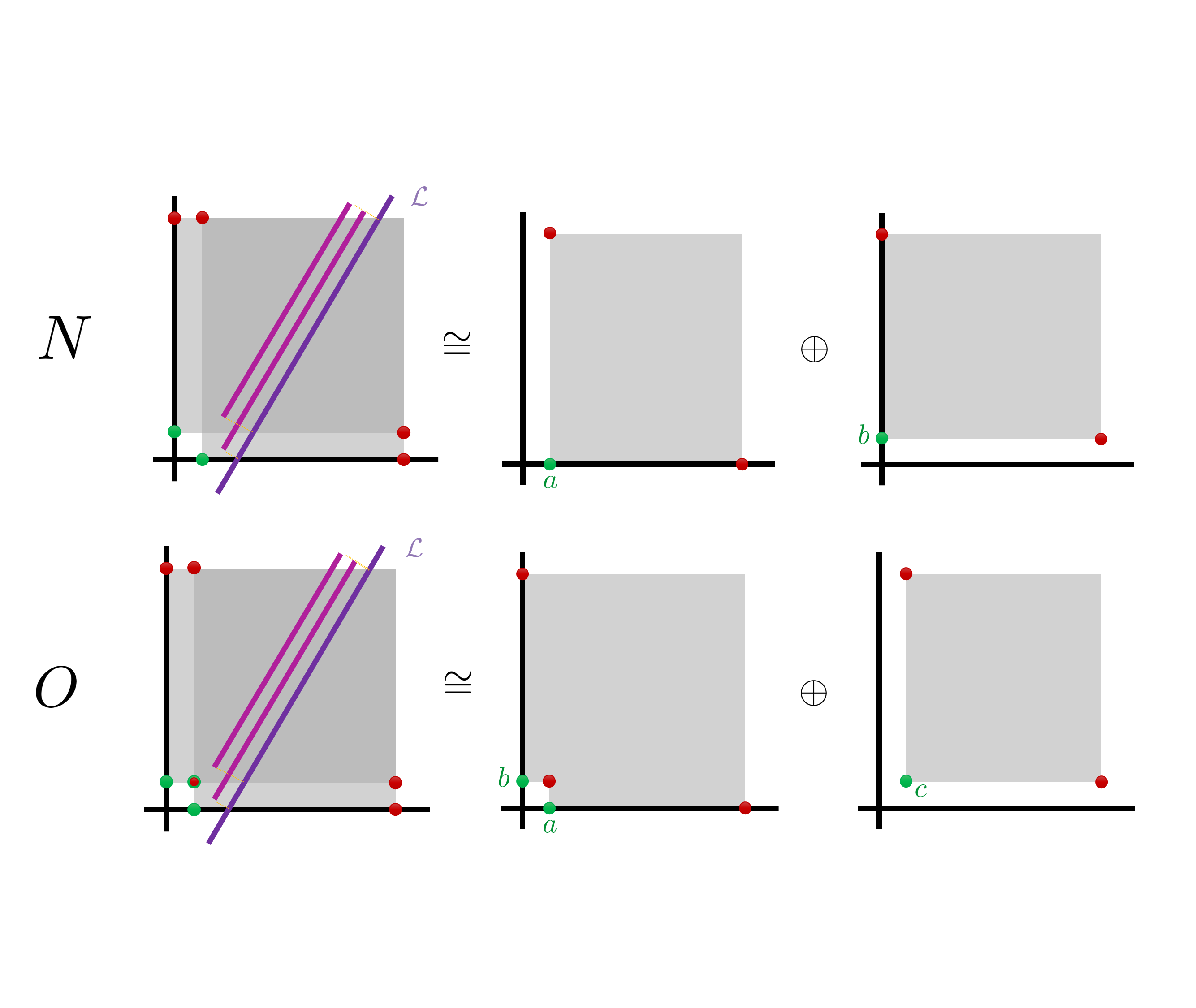
Figure 3: Non-isomorphic interval decomposable 2-parameter persistence modules NN and OO, dI​(N,O)=ε>0d_{I}(N,O)=\varepsilon>0 2.1. The fibered bar codes of NN and OO are identical and thus the matching distance between NN and OO is zero, d0​(N,O)=0d_{0}(N,O)=0.
Example 2.1 (Incompleteness of the Matching Distance).

Let us define the following graded sets and homogeneous subset:

𝒳N\displaystyle\mathcal{X}_{N} ={(a,(ε,0)),(b,(0,ε))}\displaystyle=\{(a,(\varepsilon,0)),(b,(0,\varepsilon))\}
𝒳O\displaystyle\mathcal{X}_{O} =𝒳N∪{(c,(ε,ε))}\displaystyle=\mathcal{X}_{N}\cup\{(c,(\varepsilon,\varepsilon))\}
ℛN\displaystyle\mathcal{R}_{N} ={x19​ε⋅a,x29​ε⋅b,x210​ε⋅a,x110​ε⋅b}⊂Free​[𝒳N]\displaystyle=\{x_{1}^{9\varepsilon}\cdot a,x_{2}^{9\varepsilon}\cdot b,x_{2}^{10\varepsilon}\cdot a,x_{1}^{10\varepsilon}\cdot b\}\subset\text{Free}[\mathcal{X}_{N}]
ℛO\displaystyle\mathcal{R}_{O} =ℛO∪{x1ε⋅b−x2ε⋅a,x19​ε⋅c,x29​ε⋅c}⊂Free​[𝒳O]\displaystyle=\mathcal{R}_{O}\cup\{x_{1}^{\varepsilon}\cdot b-x_{2}^{\varepsilon}\cdot a,x_{1}^{9\varepsilon}\cdot c,x_{2}^{9\varepsilon}\cdot c\}\subset\text{Free}[\mathcal{X}_{O}]

Let N,ON,O denote the 2-parameter persistence modules with presentations ⟨𝒳N|ℛN⟩,⟨𝒳O|ℛO⟩\langle\mathcal{X}_{N}|\mathcal{R}_{N}\rangle,\langle\mathcal{X}_{O}|\mathcal{R}_{O}\rangle respectively (see Figure 3). The fibered bar code of NN and OO are indistinguishable, d0​(N,O)=0d_{0}(N,O)=0, yet dI​(N,O)=εd_{I}(N,O)=\varepsilon. We also have that dI​(N,0),dI​(O,0)≤5​εd_{I}(N,0),d_{I}(O,0)\leq 5\varepsilon, so for any 2-parameter module MM, dI​(M,M⊕N),dI​(M,M⊕O)≤5​εd_{I}(M,M\oplus N),d_{I}(M,M\oplus O)\leq 5\varepsilon and d0​(M⊕N,M⊕O)=0d_{0}(M\oplus N,M\oplus O)=0. This example witnesses the incompleteness of the matching distance and shows that our local equivalence of metrics between dId_{I} and d0d_{0} (1) is necessarily anchored about MM.

Definition 2.11 (Multiparameter Betti Numbers).

Let MM be a multiparameter persistence module. The multiparameter Betti numbers are maps ξi​(M):ℝn→ℕ\xi_{i}(M):\mathbb{R}^{n}\to\mathbb{N} defined by:

ξi​(M)​(𝐚)=dim𝔽(ToriPn​(M,Pn/I​Pn)𝐚)\xi_{i}(M)(\mathbf{a})=\dim_{\mathbb{F}}(\text{Tor}^{P_{n}}_{i}(M,P_{n}/IP_{n})_{\mathbf{a}})

The multiparameter Betti numbers are well defined (see [LW15] for details).

If ⟨𝒳|ℛ⟩\langle\mathcal{X}|\mathcal{R}\rangle is a minimal presentation for MM then ξ0​(M)​(𝐚)=|gr𝒳−1​(𝐚)|\xi_{0}(M)(\mathbf{a})=|\text{gr}^{-1}_{\mathcal{X}}(\mathbf{a})| and ξ1​(M)​(𝐚)=|grℛ−1​(𝐚)|\xi_{1}(M)(\mathbf{a})=|\text{gr}^{-1}_{\mathcal{R}}(\mathbf{a})|. More generally the support of the maps ξi​(M)\xi_{i}(M) are the locations of the generators of FiF_{i} in a minimal free resolution F∙→MF_{\bullet}\to M (up to multiplicity).

For convenience we will refer to ξi​(M)\xi_{i}(M) as a set, by which we mean the support of the map ξi​(M)\xi_{i}(M). That is, when we refer to a multiparameter Betti number 𝐚∈ξi​(M)\mathbf{a}\in\xi_{i}(M) we mean that 𝐚\mathbf{a} is in the support of ξi​(M)\xi_{i}(M) and thus there is a generator at grade 𝐚\mathbf{a} in any minimal free resolution.

For a finitely presented module we can break up ℝn\mathbb{R}^{n} into cells within which the module is constant (the internal morphisms are isomorphisms). The boundaries of these cells are determined by the positions of the multiparameter Betti numbers.

Refer to caption
(a) A grid functions 𝒢:[k1]×[k2]→ℝ2\mathcal{G}:[k_{1}]\times[k_{2}]\to\mathbb{R}^{2} together with the associated collection of axis aligned lines Grid𝒢\text{Grid}_{\mathcal{G}}.
Refer to caption
(b) A grid functions 𝒢:[k1]×[k2]×[k3]→ℝ3\mathcal{G}:[k_{1}]\times[k_{2}]\times[k_{3}]\to\mathbb{R}^{3} together with the associated collection of axis aligned hyperplanes Grid𝒢\text{Grid}_{\mathcal{G}}.
Figure 4: Example grid functions with their associated collection of axis aligned hyperplanes.
Refer to caption
(a) Multiparameter Betti numbers of some 2-parameter module M∈𝐯𝐞𝐜𝐭fin𝐑2M\in\mathbf{vect}_{\text{fin}}^{\mathbf{R}^{2}} together with the collection of axis aligned lines Grid𝒢M\text{Grid}_{\mathcal{G}_{M}}.
Refer to caption
(b) Multiparameter Betti numbers of some 3-parameter module M∈𝐯𝐞𝐜𝐭fin𝐑3M\in\mathbf{vect}_{\text{fin}}^{\mathbf{R}^{3}} together with the collection of axis aligned hyperplanes Grid𝒢M\text{Grid}_{\mathcal{G}_{M}}.
Figure 5: Multiparameter Betti numbers of multiparameter persistence modules together with their associated collection of axis aligned hyperplanes.
Definition 2.12 (Grid Function).

Let [k][k] denote the set {1,…,k}\{1,...,k\}. A grid function is a map 𝒢=Πj=1n​𝒢j:Πj=1n​[kj]→ℝn\mathcal{G}=\Pi_{j=1}^{n}\mathcal{G}^{j}:\Pi_{j=1}^{n}[k_{j}]\to\mathbb{R}^{n}. We shall use Grid𝒢\text{Grid}_{\mathcal{G}} to denote the collection of axis aligned hyperplanes which passes through the image of this map:

Grid𝒢:={𝐚∈ℝn:πj​(𝐚)∈Im⁡𝒢j​ for some ​j∈[n]}\text{Grid}_{\mathcal{G}}:=\{\mathbf{a}\in\mathbb{R}^{n}:\pi_{j}(\mathbf{a})\in\Ima\mathcal{G}^{j}\text{ for some }j\in[n]\}
Definition 2.13 (Controlling Constant).

For a grid function 𝒢:Πj=1n​[kj]→ℝn\mathcal{G}:\Pi_{j=1}^{n}[k_{j}]\to\mathbb{R}^{n} we define the controlling constant c⁡(𝒢)c(\mathcal{G}) to be:

c(𝒢):=min{∥𝐚−𝐛∥∞:𝐚≠𝐛,𝐚,𝐛∈Im𝒢}c(\mathcal{G}):=\min\{\|\mathbf{a}-\mathbf{b}\|_{\infty}:\mathbf{a}\neq\mathbf{b},\mathbf{a},\mathbf{b}\in\Ima\mathcal{G}\}

In the edge cases for which Im⁡𝒢\Ima\mathcal{G} is empty or a singleton, we define the controlling constant to be infinite.

Definition 2.14 (Multiparameter Betti Grid).

Suppose M∈𝐯𝐞𝐜𝐭fin𝐑nM\in\mathbf{vect}_{\text{fin}}^{\mathbf{R}^{n}} is a finitely presented multiparameter persistence module and that the multiparameter Betti numbers ∪iξi(M)\cup_{i}\xi_{i}(M) have kjk_{j} distinct gradings in the jthj^{\text{th}}-coordinate. Let 𝒢M=Πj=1n​𝒢Mj:Πj=1n​[kj]→ℝn\mathcal{G}_{M}=\Pi_{j=1}^{n}\mathcal{G}^{j}_{M}:\Pi_{j=1}^{n}[k_{j}]\to\mathbb{R}^{n} be the map such that ∪iξi(M)⊂Im𝒢M\cup_{i}\xi_{i}(M)\subset\Ima\mathcal{G}_{M}. The image of this map shall be referred to as the multiparameter Betti grid of MM and denoted Im⁡𝒢M\Ima\mathcal{G}_{M}.

The grid Grid𝒢M\text{Grid}_{\mathcal{G}_{M}} marks the boundaries of the cells within which the module MM does not change.

For a finitely presented module M∈𝐯𝐞𝐜𝐭fin𝐑nM\in\mathbf{vect}_{\text{fin}}^{\mathbf{R}^{n}} we define the controlling constant cMc_{M} to be the controlling constant of the multiparameter Betti grid of MM, cM=c⁡(𝒢M)c_{M}=c(\mathcal{G}_{M}). This is the minimum non-zero difference between coordinates of the collection of multiparameter Betti numbers ∪iξi(M)\cup_{i}\xi_{i}(M).

Definition 2.15 (Complexity).

Suppose M∈𝐯𝐞𝐜𝐭fin𝐑nM\in\mathbf{vect}_{\text{fin}}^{\mathbf{R}^{n}} and F∙F_{\bullet} is a free resolution of MM. We define the complexity of the resolution F∙F_{\bullet} to be the cardinal 𝒞⁡(F∙)=∑i|Fi|\mathcal{C}(F_{\bullet})=\sum_{i}|F_{i}|, where |Fi||F_{i}| denotes the cardinality of the generating set of FiF_{i}. We define the complexity of the persistence module MM to be the minimal complexity of a resolution of MM, 𝒞⁡(M)=minF∙→M⁡𝒞⁡(F∙)\mathcal{C}(M)=\min_{F_{\bullet}\to M}\mathcal{C}(F_{\bullet}).

Observe that the complexity of a module MM is realised by the complexity of a minimal resolution and thus 𝒞(M)=|∪i=0nξi(M)|\mathcal{C}(M)=|\cup_{i=0}^{n}\xi_{i}(M)|.

Lemma 2.1 (Multiparameter Betti Grid is Determined by Generators and Relations).

Let M∈𝐯𝐞𝐜𝐭fin𝐑nM\in\mathbf{vect}_{\text{fin}}^{\mathbf{R}^{n}} be a finitely presented multiparameter persistence module. For all j≥1j\geq 1 if 𝐬∈ξj+1​(M)\mathbf{s}\in\xi_{j+1}(M) then there exist 𝐫i∈ξj​(M)\mathbf{r}_{i}\in\xi_{j}(M) such that 𝐬=⋁i𝐫i\mathbf{s}=\bigvee_{i}\mathbf{r}_{i}. Thus the the multiparameter Betti grid of MM is determined by ξ0​(M)∪ξ1​(M)\xi_{0}(M)\cup\xi_{1}(M).

Proof.

We will just prove the result for j=1j=1, since the result for j>1j>1 follows identically. Let F∙F_{\bullet} be a minimal resolution of M∈𝐯𝐞𝐜𝐭fin𝐑nM\in\mathbf{vect}_{\text{fin}}^{\mathbf{R}^{n}}. So that in particular F2↠ker⁡(p1)=ker⁡(F1→F0)F_{2}\twoheadrightarrow\ker(p_{1})=\ker(F_{1}\to F_{0}). Let F1F_{1} have generating set {𝐫i}i=1k1\{\mathbf{r}_{i}\}_{i=1}^{k_{1}}. Suppose p2​(𝐬)=∑iμi​𝐱𝐬−𝐫i⋅𝐫i∈ker⁡(p1)p_{2}(\mathbf{s})=\sum_{i}\mu_{i}\mathbf{x}^{\mathbf{s}-\mathbf{r}_{i}}\cdot\mathbf{r}_{i}\in\ker(p_{1}). Note that we must have 𝐬≥⋁j:μj≠0𝐫j\mathbf{s}\geq\bigvee_{j:\mu_{j}\neq 0}\mathbf{r}_{j}. Suppose 𝐬>⋁j:μj≠0𝐫j\mathbf{s}>\bigvee_{j:\mu_{j}\neq 0}\mathbf{r}_{j}. We observe that

0=p1(p2(𝐬))=p1(𝐱𝐬−⋁j:μj≠0𝐫j⋅∑iμi𝐱⋁j:μj≠0𝐫j−𝐫i⋅𝐫i)=𝐱𝐬−⋁j:μj≠0𝐫j⋅p1(∑iμi𝐱⋁j:μj≠0𝐫j−𝐫i⋅𝐫i)0=p_{1}(p_{2}(\mathbf{s}))=p_{1}(\mathbf{x}^{\mathbf{s}-\bigvee_{j:\mu_{j}\neq 0}\mathbf{r}_{j}}\cdot\sum_{i}\mu_{i}\mathbf{x}^{\bigvee_{j:\mu_{j}\neq 0}\mathbf{r}_{j}-\mathbf{r}_{i}}\cdot\mathbf{r}_{i})=\mathbf{x}^{\mathbf{s}-\bigvee_{j:\mu_{j}\neq 0}\mathbf{r}_{j}}\cdot p_{1}(\sum_{i}\mu_{i}\mathbf{x}^{\bigvee_{j:\mu_{j}\neq 0}\mathbf{r}_{j}-\mathbf{r}_{i}}\cdot\mathbf{r}_{i})

Since F0F_{0} is free it follows that p1(∑iμi𝐱⋁j:μj≠0𝐫j−𝐫i⋅𝐫i)=0p_{1}(\sum_{i}\mu_{i}\mathbf{x}^{\bigvee_{j:\mu_{j}\neq 0}\mathbf{r}_{j}-\mathbf{r}_{i}}\cdot\mathbf{r}_{i})=0 and hence there is some element m∈F2{m}\in F_{2} with p2(m)=∑iμi𝐱⋁j:μj≠0𝐫j−𝐫i⋅𝐫ip_{2}({m})=\sum_{i}\mu_{i}\mathbf{x}^{\bigvee_{j:\mu_{j}\neq 0}\mathbf{r}_{j}-\mathbf{r}_{i}}\cdot\mathbf{r}_{i}. Thus 𝐬−𝐱𝐬−⋁j:μj≠0𝐫j⋅m∈ker(p2)\mathbf{s}-\mathbf{x}^{\mathbf{s}-\bigvee_{j:\mu_{j}\neq 0}\mathbf{r}_{j}}\cdot{m}\in\ker(p_{2}) and so 𝐬∉ξ2​(M)\mathbf{s}\not\in\xi_{2}(M) else we contradict minimality of the resolution F∙F_{\bullet}. ∎

The following 2.2 gives a simple criterion for reducing the complexity of a resolution. Let ⟨⋅,⋅⟩\langle\cdot,\cdot\rangle denote the point-wise vector space inner product of a finitely generated free module which makes it’s generating set an orthonormal basis.

Lemma 2.2 (Cancellation Lemma).

Let M∈𝐯𝐞𝐜𝐭fin𝐑nM\in\mathbf{vect}_{\text{fin}}^{\mathbf{R}^{n}} be a finitely presented multiparameter persistence module. Suppose F∙→MF_{\bullet}\to M is a free resolution such that there exists a generator 𝐛\mathbf{b} of FiF_{i}, and a generator 𝐫𝐛\mathbf{r}_{\mathbf{b}} of Fi+1F_{i+1} with grade​(𝐛)=grade​(𝐫𝐛)\text{grade}(\mathbf{b})=\text{grade}(\mathbf{r}_{\mathbf{b}}) and ⟨pi+1​(𝐫𝐛),𝐛⟩≠0\langle p_{i+1}(\mathbf{r}_{\mathbf{b}}),\mathbf{b}\rangle\neq 0, then F∙F_{\bullet} is not a minimal resolution, and there is a free resolution F∙′→MF_{\bullet}^{\prime}\to M with ξ0​(Fi+1′)=ξ0​(Fi+1)∖{𝐫𝐛}\xi_{0}(F^{\prime}_{i+1})=\xi_{0}(F_{i+1})\setminus\{\mathbf{r}_{\mathbf{b}}\} and ξ0​(Fi′)=ξ0​(Fi)∖{𝐛}\xi_{0}(F^{\prime}_{i})=\xi_{0}(F_{i})\setminus\{\mathbf{b}\}. That is to say we may cancel the pair of generators 𝐛\mathbf{b} and 𝐫𝐛\mathbf{r}_{\mathbf{b}} in the resolution.

Proof.

Let F∙′F^{\prime}_{\bullet} denote the chain complex of free modules for which ξ0​(Fi+1′)=ξ0​(Fi+1)∖{𝐫𝐛}\xi_{0}(F^{\prime}_{i+1})=\xi_{0}(F_{i+1})\setminus\{\mathbf{r}_{\mathbf{b}}\}, ξ0​(Fi′)=ξ0​(Fi)∖{𝐛}\xi_{0}(F^{\prime}_{i})=\xi_{0}(F_{i})\setminus\{\mathbf{b}\} and ξ0​(Fj′)=ξ0​(Fj)\xi_{0}(F^{\prime}_{j})=\xi_{0}(F_{j}) otherwise, with morphisms inherited from F∙F_{\bullet}. Define chain maps f:F∙→F∙′f:F_{\bullet}\to F^{\prime}_{\bullet} and g:F∙′→F∙g:F^{\prime}_{\bullet}\to F_{\bullet} to be the identity on 𝐚∉{𝐫𝐛,𝐛}\mathbf{a}\not\in\{\mathbf{r}_{\mathbf{b}},\mathbf{b}\}; (fi​(𝐚)=𝐚f_{i}(\mathbf{a})=\mathbf{a}, gi​(𝐚)=𝐚g_{i}(\mathbf{a})=\mathbf{a}). Define fi+1​(𝐫𝐛)=0f_{i+1}(\mathbf{r}_{\mathbf{b}})=0 and fi​(𝐛)=𝐛−1⟨pi+1​(𝐫𝐛),𝐛⟩​pi+1​(𝐫𝐛)f_{i}(\mathbf{b})=\mathbf{b}-\frac{1}{\langle p_{i+1}(\mathbf{r}_{\mathbf{b}}),\mathbf{b}\rangle}p_{i+1}(\mathbf{r}_{\mathbf{b}}). Then we observe that f∘g=idF∙′f\circ g=\id_{F^{\prime}_{\bullet}} and, g∘f≃idF∙g\circ f\simeq\id_{F_{\bullet}} is realised by the homotopy H:F∙→F∙+1H:F_{\bullet}\to F_{\bullet+1} which is zero everywhere except Hi​(𝐛)=1⟨pi+1​(𝐫𝐛),𝐛⟩​𝐫𝐛H_{i}(\mathbf{b})=\frac{1}{\langle p_{i+1}(\mathbf{r}_{\mathbf{b}}),\mathbf{b}\rangle}\mathbf{r}_{\mathbf{b}}. Indeed pi+1∘Hi​(𝐛)=1⟨pi+1​(𝐫𝐛),𝐛⟩​pi+1​(𝐫𝐛)=(idFi−gi∘fi)​(𝐛)p_{i+1}\circ H_{i}(\mathbf{b})=\frac{1}{\langle p_{i+1}(\mathbf{r}_{\mathbf{b}}),\mathbf{b}\rangle}p_{i+1}(\mathbf{r}_{\mathbf{b}})=(\id_{F_{i}}-g_{i}\circ f_{i})(\mathbf{b}) and Hi+1∘pi+1​(𝐫𝐛)=Hi+1​(⟨pi+1​(𝐫𝐛),𝐛⟩​𝐛)=𝐫𝐛=(idFi+1−gi+1∘fi+1)​(𝐫𝐛)H_{i+1}\circ p_{i+1}(\mathbf{r}_{\mathbf{b}})=H_{i+1}(\langle p_{i+1}(\mathbf{r}_{\mathbf{b}}),\mathbf{b}\rangle\mathbf{b})=\mathbf{r}_{\mathbf{b}}=(\id_{F_{i+1}}-g_{i+1}\circ f_{i+1})(\mathbf{r}_{\mathbf{b}}). ∎

3 Merge and Simplification Functors

In this Section we define two families of endofunctors acting on 𝐯𝐞𝐜𝐭fin𝐑n\mathbf{vect}_{\text{fin}}^{\mathbf{R}^{n}}. These functors will be used in the proof of our main result 4.1. We shall show that these functors are well-defined and explicit how these functors affect the presentation of a module.

Notation

Let us establish some notation conventions for this section. We shall denote free multigraded module resolutions as (F∙,p∙)(F_{\bullet},p_{\bullet}) where pi:Fi→Fi−1p_{i}:F_{i}\to F_{i-1}. We shall denote generators of F0F_{0} using the letter 𝐛\mathbf{b} for “births” and we shall denote generators of F1F_{1} using the letter 𝐫\mathbf{r} for “relations”. We shall simultaneously use 𝐛\mathbf{b} to denote both the generator (an element of a graded set) and its grading. If there is ambiguity we shall explicitly write gr​(𝐛)\text{gr}(\mathbf{b}) to denote the grading. Given an element 𝐚∈ℝn\mathbf{a}\in\mathbb{R}^{n} we will denote the slope 𝟏\mathbf{1} line through 𝐚\mathbf{a} as ℒ𝐚\mathcal{L}_{\mathbf{a}} with ℒ𝐚​(0)=𝐚\mathcal{L}_{\mathbf{a}}(0)=\mathbf{a} and the isometric embedding with respect to ∥⋅∥∞\|\cdot\|_{\infty}. For a set S⊂ℝnS\subset\mathbb{R}^{n} and 𝐚∈ℝn\mathbf{a}\in\mathbb{R}^{n} we use the shorthand ‖𝐚−S‖∞:=inf𝐬∈S‖𝐚−𝐬‖∞\|\mathbf{a}-S\|_{\infty}:=\inf_{\mathbf{s}\in S}\|\mathbf{a}-\mathbf{s}\|_{\infty}.

3.1 Merge Functor

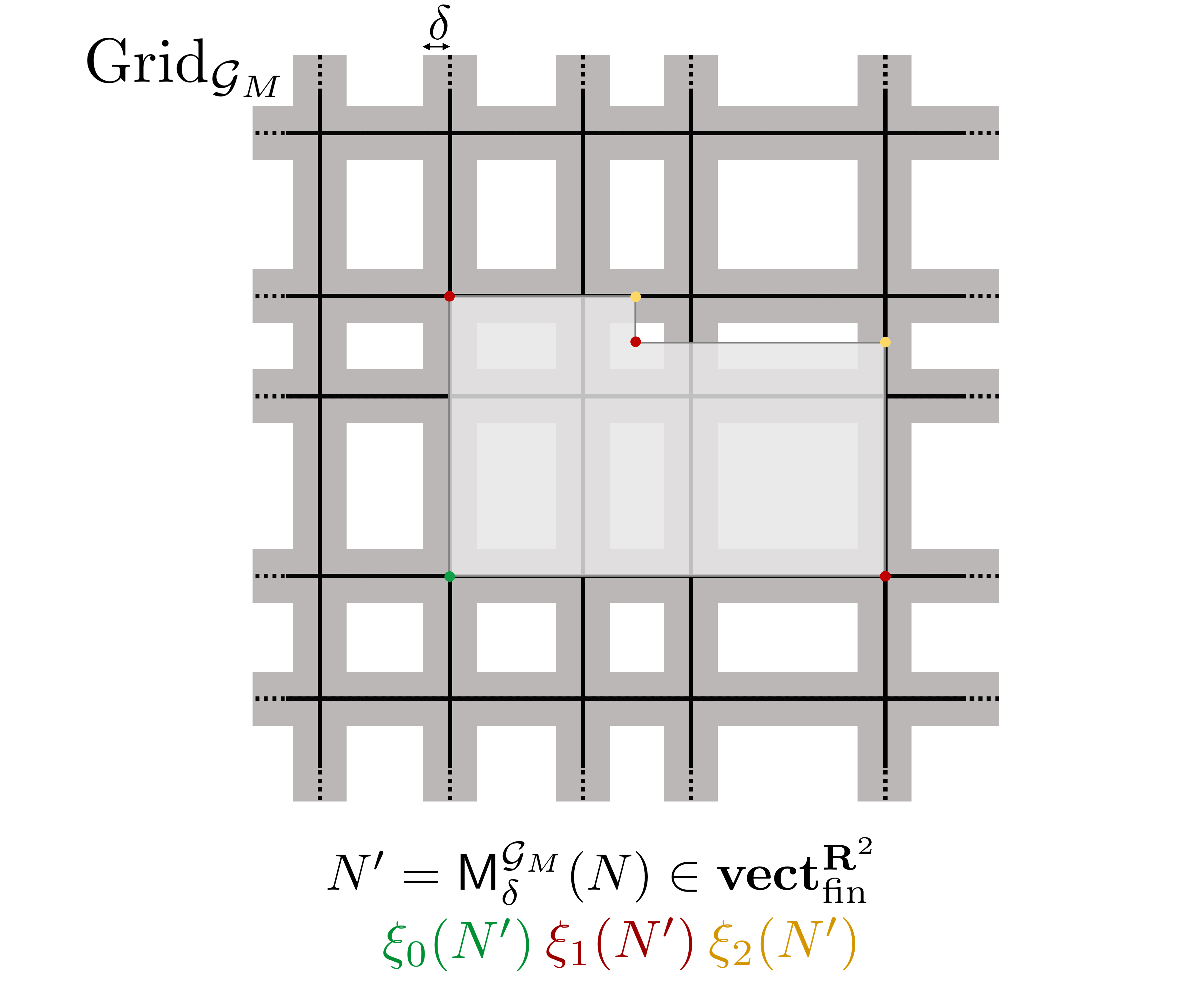
The first family of functors we define we call merge functors. These are analogous to the merge operations defined in [CO18] for Reeb graphs which are heavily used in [CO17]. Figure 6 gives a pictorial description of the action of a merge functor on a multiparameter module. The merge functor moves the grades of multiparameter Betti numbers lying close to a grid to lie on that grid. Moving the multiparameter Betti numbers may cause cancellations (2.2).

We give a module-theoretic and category-theoretic formulation of the merge functor and establish that these formulations are equivalent. The module-theoretic formulation clarifies how the functor changes the presentation of a module, whilst the category-theoretic formulation establishes the functoriality and exactness of the merge functor immediately.

Refer to caption
(a)
Refer to caption
(b)
Figure 6: An example of a module under a Merge functor. In (a) we depict an interval module NN overlayed on the δ\delta-neighbourhood of the grid Grid𝒢M\text{Grid}_{\mathcal{G}_{M}}, with the multiparameter Betti numbers of NN marked. We observe cancellations of the multiparameter Betti numbers under the Merge functor Mδ𝒢M\textsf{M}_{\delta}^{\mathcal{G}_{M}}, and the multiparameter Betti numbers of NN lying δ\delta-close to the grid are merged to lie on the grid.
Definition 3.1 (Merge Functions).

Let 𝒢:[k]→ℝ\mathcal{G}:[k]\to\mathbb{R} be a finite grid with controlling constant cc, and let δ<c2\delta<\frac{c}{2}. Define the merge functions Mδ𝒢:ℝ→ℝ\textsf{M}_{\delta}^{\mathcal{G}}:\mathbb{R}\to\mathbb{R}, Mδ𝒢+:ℝ→ℝ\textsf{M}_{\delta}^{\mathcal{G}_{+}}:\mathbb{R}\to\mathbb{R}, Mδ𝒢−:ℝ→ℝ\textsf{M}_{\delta}^{\mathcal{G}_{-}}:\mathbb{R}\to\mathbb{R} as follows:

Mδ𝒢​(x)\displaystyle\textsf{M}_{\delta}^{\mathcal{G}}(x) ={𝒢⁡(i) if ​x∈[𝒢⁡(i)−δ,𝒢⁡(i)+δ]x otherwise\displaystyle=\begin{cases}\mathcal{G}(i)&\text{ if }x\in[\mathcal{G}(i)-\delta,\mathcal{G}(i)+\delta]\\ x&\text{ otherwise}\end{cases}
Mδ𝒢+​(x)\displaystyle\textsf{M}_{\delta}^{\mathcal{G}_{+}}(x) ={𝒢⁡(i) if ​x∈[𝒢⁡(i)−δ,𝒢⁡(i)]x otherwise\displaystyle=\begin{cases}\mathcal{G}(i)&\text{ if }x\in[\mathcal{G}(i)-\delta,\mathcal{G}(i)]\\ x&\text{ otherwise}\end{cases}
Mδ𝒢−​(x)\displaystyle\textsf{M}_{\delta}^{\mathcal{G}_{-}}(x) ={𝒢⁡(i) if ​x∈[𝒢⁡(i),𝒢⁡(i)+δ]x otherwise\displaystyle=\begin{cases}\mathcal{G}(i)&\text{ if }x\in[\mathcal{G}(i),\mathcal{G}(i)+\delta]\\ x&\text{ otherwise}\end{cases}

Note that Mδ𝒢=Mδ𝒢−∘Mδ𝒢+\textsf{M}_{\delta}^{\mathcal{G}}=\textsf{M}_{\delta}^{\mathcal{G}_{-}}\circ\textsf{M}_{\delta}^{\mathcal{G}_{+}} and the merge functions are projections.

For a multiparameter grid function 𝒢=𝒢1×…×𝒢n\mathcal{G}=\mathcal{G}^{1}\times...\times\mathcal{G}^{n} with controlling constant cc and δ<c2\delta<\frac{c}{2}. The function Mδ𝒢:ℝn→ℝn\textsf{M}_{\delta}^{\mathcal{G}}:\mathbb{R}^{n}\to\mathbb{R}^{n} is defined using the merge functions Mδ𝒢i\textsf{M}_{\delta}^{\mathcal{G}_{i}} coordinate-wise, and similarly for Mδ𝒢+\textsf{M}_{\delta}^{\mathcal{G}_{+}} and Mδ𝒢−\textsf{M}_{\delta}^{\mathcal{G}_{-}}

Note that a merge function preserves the partial order of a pair of elements in ℝn\mathbb{R}^{n}. That is to say 𝐚≤𝐛\mathbf{a}\leq\mathbf{b} implies Mδ𝒢​(𝐚)≤Mδ𝒢​(𝐛)\textsf{M}_{\delta}^{\mathcal{G}}(\mathbf{a})\leq\textsf{M}_{\delta}^{\mathcal{G}}(\mathbf{b}). We first define the action of the merge functor on free modules.

Definition 3.2 (Merge Functor for Free Modules).

Let 𝒢=Πi=1n​𝒢i:Πi=1n​[ki]→ℝn\mathcal{G}=\Pi_{i=1}^{n}\mathcal{G}^{i}:\Pi_{i=1}^{n}[k_{i}]\to\mathbb{R}^{n} be a grid with separation constant cc, and let δ<c2\delta<\frac{c}{2}. We define the δ\delta-merge of the free module F=Free​[𝒳]F=\text{Free}[\mathcal{X}] with respect to the grid 𝒢\mathcal{G} to be the free module with grading set regraded via the merge function: Mδ𝒢​(F)=Free​[Mδ𝒢​(𝒳)]\textsf{M}_{\delta}^{\mathcal{G}}(F)=\text{Free}[\textsf{M}_{\delta}^{\mathcal{G}}(\mathcal{X})], together with the obvious action on morphisms of free modules.

Since the merge function preserves the partial order on ℝn\mathbb{R}^{n}, Mδ𝒢\textsf{M}_{\delta}^{\mathcal{G}} is well defined on morphisms of free modules. It is straight forward to check that Mδ𝒢\textsf{M}_{\delta}^{\mathcal{G}} respects identity morphisms for free modules and compositions of morphisms between free modules.

Definition 3.3 (Merge Functor).

Let M∈𝐯𝐞𝐜𝐭fin𝐑nM\in\mathbf{vect}_{\text{fin}}^{\mathbf{R}^{n}} and 𝒢=Πi=1n​𝒢i:Πi=1n​[ki]→ℝn\mathcal{G}=\Pi_{i=1}^{n}\mathcal{G}^{i}:\Pi_{i=1}^{n}[k_{i}]\to\mathbb{R}^{n} a grid with separation constant cc, and let δ<c2\delta<\frac{c}{2}. Suppose F1→F0→MF_{1}\to F_{0}\to M is a presentation of MM. We define the δ\delta-merge of the module MM with respect to the grid 𝒢\mathcal{G} to be the module coker Mδ𝒢​(F1→F0)\text{coker }\textsf{M}_{\delta}^{\mathcal{G}}(F_{1}\to F_{0}) i.e. the module Mδ𝒢​(M)\textsf{M}_{\delta}^{\mathcal{G}}(M) with presentation:

Mδ𝒢​(F1)→Mδ𝒢​(F0)→Mδ𝒢​(M)\textsf{M}_{\delta}^{\mathcal{G}}(F_{1})\to\textsf{M}_{\delta}^{\mathcal{G}}(F_{0})\to\textsf{M}_{\delta}^{\mathcal{G}}(M)

We define Mδ𝒢\textsf{M}_{\delta}^{\mathcal{G}} on a morphism of multiparameter persistence modules f:M→Nf:M\to N to be the morphism induced from Mδ𝒢\textsf{M}_{\delta}^{\mathcal{G}} applied to the free module morphism f0f_{0}, (the lift of ff between the free modules generating MM and NN).

Proposition 3.1 (Merge Functor is Well-defined).

Mδ𝒢\textsf{M}_{\delta}^{\mathcal{G}} is a well-defined endofunctor on the category 𝐯𝐞𝐜𝐭fin𝐑n\mathbf{vect}_{\text{fin}}^{\mathbf{R}^{n}} for all δ<c2\delta<\frac{c}{2}.

Proof.

We first observe that Mδ𝒢\textsf{M}_{\delta}^{\mathcal{G}} is independent of the presentation chosen. Any presentation gives rise to a free resolution and two such free resolutions of a module are homotopy equivalent. Since Mδ𝒢\textsf{M}_{\delta}^{\mathcal{G}} respects compositions and identity maps of free modules the free resolutions under the map Mδ𝒢\textsf{M}_{\delta}^{\mathcal{G}} remain homotopy equivalent.

Let us now show that Mδ𝒢\textsf{M}_{\delta}^{\mathcal{G}} is well defined on morphisms. Suppose f:M→Nf:M\to N is a morphism of modules, and suppose F1→F0→MF_{1}\to F_{0}\to M is a presentation of MM and G1→G0→NG_{1}\to G_{0}\to N is a presentation of NN. Note that ff lifts to a chain map between these presentations:

F1{\lx@inpgf@ignorespaces F_{1}}F0{\lx@inpgf@ignorespaces F_{0}}M{\lx@inpgf@ignorespaces M}G1{\lx@inpgf@ignorespaces G_{1}}G0{\lx@inpgf@ignorespaces G_{0}}N{\lx@inpgf@ignorespaces N}f1\scriptstyle{\lx@inpgf@ignorespaces f_{1}}p1\scriptstyle{\lx@inpgf@ignorespaces p_{1}}f0\scriptstyle{\lx@inpgf@ignorespaces f_{0}}p0\scriptstyle{\lx@inpgf@ignorespaces p_{0}}f\scriptstyle{\lx@inpgf@ignorespaces f}q1\scriptstyle{\lx@inpgf@ignorespaces q_{1}}q0\scriptstyle{\lx@inpgf@ignorespaces q_{0}}

Let F0=Free​({𝐛iM})F_{0}=\text{Free}(\{\mathbf{b}^{M}_{i}\}), G0=Free​({𝐛jN})G_{0}=\text{Free}(\{\mathbf{b}^{N}_{j}\}), F1=Free​({𝐫lM})F_{1}=\text{Free}(\{\mathbf{r}^{M}_{l}\}), G1=Free​({𝐫mN})G_{1}=\text{Free}(\{\mathbf{r}^{N}_{m}\}), and recall that ff is determined by the action of f0f_{0} on the generators {𝐛iM}\{\mathbf{b}^{M}_{i}\}. Suppose that f0​(𝐛iM)=∑jci,j​𝐱𝐛iM−𝐛jN⋅𝐛jNf_{0}(\mathbf{b}^{M}_{i})=\sum_{j}c_{i,j}\mathbf{x}^{\mathbf{b}^{M}_{i}-\mathbf{b}^{N}_{j}}\cdot\mathbf{b}^{N}_{j} The morphism Mδ𝒢​(f):Mδ𝒢​(M)→Mδ𝒢​(N)\textsf{M}_{\delta}^{\mathcal{G}}(f):\textsf{M}_{\delta}^{\mathcal{G}}(M)\to\textsf{M}_{\delta}^{\mathcal{G}}(N) is defined to act on generators as:

Mδ𝒢​(f)​(Mδ𝒢​(𝐛iM))=∑jci,j​𝐱Mδ𝒢​(𝐛iM)−Mδ𝒢​(𝐛jN)⋅Mδ𝒢​(𝐛jN)\textsf{M}_{\delta}^{\mathcal{G}}(f)(\textsf{M}_{\delta}^{\mathcal{G}}(\mathbf{b}^{M}_{i}))=\sum_{j}c_{i,j}\mathbf{x}^{\textsf{M}_{\delta}^{\mathcal{G}}(\mathbf{b}^{M}_{i})-\textsf{M}_{\delta}^{\mathcal{G}}(\mathbf{b}^{N}_{j})}\cdot\textsf{M}_{\delta}^{\mathcal{G}}(\mathbf{b}^{N}_{j})

To check Mδ𝒢​(f)\textsf{M}_{\delta}^{\mathcal{G}}(f) is well defined for arbitrary ff it suffices to show that Mδ𝒢​(f0∘p1)​(Mδ𝒢​(𝐫lM))∈Im⁡Mδ𝒢​(q1)\textsf{M}_{\delta}^{\mathcal{G}}(f_{0}\circ p_{1})(\textsf{M}_{\delta}^{\mathcal{G}}(\mathbf{r}^{M}_{l}))\in\Ima\textsf{M}_{\delta}^{\mathcal{G}}(q_{1}). As ff is well defined we have that f0∘p1​(𝐫lM)∈Im⁡q1f_{0}\circ p_{1}(\mathbf{r}^{M}_{l})\in\Ima q_{1}:

f0∘p1​(𝐫lM)\displaystyle f_{0}\circ p_{1}(\mathbf{r}^{M}_{l}) =f0​(∑icl,i​𝐱𝐫lM−𝐛iM⋅𝐛iM)=∑j∑ici,j​cl,i​𝐱𝐫lM−𝐛jN⋅𝐛jN\displaystyle=f_{0}(\sum_{i}c_{l,i}\mathbf{x}^{\mathbf{r}^{M}_{l}-\mathbf{b}^{M}_{i}}\cdot\mathbf{b}^{M}_{i})=\sum_{j}\sum_{i}c_{i,j}c_{l,i}\mathbf{x}^{\mathbf{r}^{M}_{l}-\mathbf{b}^{N}_{j}}\cdot\mathbf{b}^{N}_{j}
=q1​(∑mam​𝐱𝐫lM−𝐫mN⋅𝐫mN)=∑j∑mam​cm,j​𝐱𝐫mN−𝐛jN⋅𝐛jN\displaystyle=q_{1}(\sum_{m}a_{m}\mathbf{x}^{\mathbf{r}^{M}_{l}-\mathbf{r}^{N}_{m}}\cdot\mathbf{r}^{N}_{m})=\sum_{j}\sum_{m}a_{m}c_{m,j}\mathbf{x}^{\mathbf{r}^{N}_{m}-\mathbf{b}^{N}_{j}}\cdot\mathbf{b}^{N}_{j}

For some scalars ama_{m}. It follows that:

Mδ𝒢​(f0∘p1)​(Mδ𝒢​(𝐫lM))\displaystyle\textsf{M}_{\delta}^{\mathcal{G}}(f_{0}\circ p_{1})(\textsf{M}_{\delta}^{\mathcal{G}}(\mathbf{r}^{M}_{l})) =∑j∑mam​cm,j​𝐱Mδ𝒢​(𝐫mN)−Mδ𝒢​(𝐛jN)⋅Mδ𝒢​(𝐛jN)\displaystyle=\sum_{j}\sum_{m}a_{m}c_{m,j}\mathbf{x}^{\textsf{M}_{\delta}^{\mathcal{G}}(\mathbf{r}^{N}_{m})-\textsf{M}_{\delta}^{\mathcal{G}}(\mathbf{b}^{N}_{j})}\cdot\textsf{M}_{\delta}^{\mathcal{G}}(\mathbf{b}^{N}_{j})
=Mδ𝒢​(q1)​(∑mam​𝐱Mδ𝒢​(𝐫lM)−Mδ𝒢​(𝐫mN)⋅Mδ𝒢​(𝐫mN))\displaystyle=\textsf{M}_{\delta}^{\mathcal{G}}(q_{1})(\sum_{m}a_{m}\mathbf{x}^{\textsf{M}_{\delta}^{\mathcal{G}}(\mathbf{r}^{M}_{l})-\textsf{M}_{\delta}^{\mathcal{G}}(\mathbf{r}^{N}_{m})}\cdot\textsf{M}_{\delta}^{\mathcal{G}}(\mathbf{r}^{N}_{m}))

and hence Mδ𝒢​(f)\textsf{M}_{\delta}^{\mathcal{G}}(f) is well defined.

∎

Another important property of the family of merge endofunctors is that Mδ𝒢\textsf{M}_{\delta}^{\mathcal{G}} perturbs multiparameter persistence modules by no more than δ\delta in the interleaving distance.

Proposition 3.2 (dI​(Mδ𝒢​(M),M)≤δd_{I}(\textsf{M}_{\delta}^{\mathcal{G}}(M),M)\leq\delta).

For any grid 𝒢\mathcal{G} and δ<c⁡(𝒢)2\delta<\frac{c(\mathcal{G})}{2}, if M∈𝐯𝐞𝐜𝐭fin𝐑nM\in\mathbf{vect}_{\text{fin}}^{\mathbf{R}^{n}} then dI​(Mδ𝒢​(M),M)≤δd_{I}(\textsf{M}_{\delta}^{\mathcal{G}}(M),M)\leq\delta.

Proof.

We will show that dI​(Mδ𝒢​(M),M)≤δd_{I}(\textsf{M}_{\delta}^{\mathcal{G}}(M),M)\leq\delta via an explicit interleaving. Let F1→p1F0→p0MF_{1}\to_{p_{1}}F_{0}\to_{p_{0}}M be a presentation of MM where F0F_{0} is free on the set {𝐛i}\{\mathbf{b}_{i}\} and F1F_{1} is free on the set {𝐫j}\{\mathbf{r}_{j}\}. Consider the maps f:M→Mδ𝒢​(M)​Tδf:M\to\textsf{M}_{\delta}^{\mathcal{G}}(M)T_{\delta} and g:Mδ𝒢​(M)→M​Tδg:\textsf{M}_{\delta}^{\mathcal{G}}(M)\to MT_{\delta} defined on generators by:

f⁡(𝐛i)=𝐱δ​𝟏+(𝐛i−Mδ𝒢​(𝐛i))⋅Mδ𝒢​(𝐛i),g⁡(Mδ𝒢​(𝐛i))=𝐱δ​𝟏+((Mδ𝒢​(𝐛i)−𝐛i)CLOSE⋅𝐛if(\mathbf{b}_{i})=\mathbf{x}^{\delta\mathbf{1}+(\mathbf{b}_{i}-\textsf{M}_{\delta}^{\mathcal{G}}(\mathbf{b}_{i}))}\cdot\textsf{M}_{\delta}^{\mathcal{G}}(\mathbf{b}_{i}),\ g(\textsf{M}_{\delta}^{\mathcal{G}}(\mathbf{b}_{i}))=\mathbf{x}^{\delta\mathbf{1}+((\textsf{M}_{\delta}^{\mathcal{G}}(\mathbf{b}_{i})-\mathbf{b}_{i})}\cdot\mathbf{b}_{i}

If these morphisms are well-defined it is clear they comprise a δ\delta-interleaving since their composition yields g∘f⁡(𝐛i)=𝐱2​δ​𝟏⋅𝐛ig\circ f(\mathbf{b}_{i})=\mathbf{x}^{2\delta\mathbf{1}}\cdot\mathbf{b}_{i} and f∘g⁡(Mδ𝒢​(𝐛i))=𝐱2​δ​𝟏⋅Mδ𝒢​(𝐛i)f\circ g(\textsf{M}_{\delta}^{\mathcal{G}}(\mathbf{b}_{i}))=\mathbf{x}^{2\delta\mathbf{1}}\cdot\textsf{M}_{\delta}^{\mathcal{G}}(\mathbf{b}_{i}). Observe that δ​𝟏≥𝐛i−Mδ𝒢​(𝐛i)≥−δ​𝟏\delta\mathbf{1}\geq\mathbf{b}_{i}-\textsf{M}_{\delta}^{\mathcal{G}}(\mathbf{b}_{i})\geq-\delta\mathbf{1} and so it suffices to check that the proposed morphisms respect relations. If ∑iαi​𝐱𝐬−𝐛i​𝐛i∈Im⁡(p1)\sum_{i}\alpha_{i}\mathbf{x}^{\mathbf{s}-\mathbf{b}_{i}}\mathbf{b}_{i}\in\Ima(p_{1}) then ∑iαi​𝐱𝐬−𝐛i​𝐛i=∑jλj​𝐱𝐬−𝐫j​p1​(𝐫j)\sum_{i}\alpha_{i}\mathbf{x}^{\mathbf{s}-\mathbf{b}_{i}}\mathbf{b}_{i}=\sum_{j}\lambda_{j}\mathbf{x}^{\mathbf{s}-\mathbf{r}_{j}}p_{1}(\mathbf{r}_{j}) for some scalars λj\lambda_{j}. We observe that:

f⁡(∑iαi​𝐱𝐬−𝐛i​𝐛i)\displaystyle f(\sum_{i}\alpha_{i}\mathbf{x}^{\mathbf{s}-\mathbf{b}_{i}}\mathbf{b}_{i}) =∑iαi​𝐱𝐬−𝐛i+δ​𝟏+(𝐛i−Mδ𝒢​(𝐛i))⋅Mδ𝒢​(𝐛i)\displaystyle=\sum_{i}\alpha_{i}\mathbf{x}^{\mathbf{s}-\mathbf{b}_{i}+\delta\mathbf{1}+(\mathbf{b}_{i}-\textsf{M}_{\delta}^{\mathcal{G}}(\mathbf{b}_{i}))}\cdot\textsf{M}_{\delta}^{\mathcal{G}}(\mathbf{b}_{i})
=∑iαi​𝐱𝐬+δ​𝟏−Mδ𝒢​(𝐛i)⋅Mδ𝒢​(𝐛i)\displaystyle=\sum_{i}\alpha_{i}\mathbf{x}^{\mathbf{s}+\delta\mathbf{1}-\textsf{M}_{\delta}^{\mathcal{G}}(\mathbf{b}_{i})}\cdot\textsf{M}_{\delta}^{\mathcal{G}}(\mathbf{b}_{i})
=∑jλj​𝐱𝐬+δ​𝟏−Mδ𝒢​(𝐫j)⋅Mδ𝒢​(p1)​(Mδ𝒢​(𝐫j))∈Im⁡(Mδ𝒢​(p1))\displaystyle=\sum_{j}\lambda_{j}\mathbf{x}^{\mathbf{s}+\delta\mathbf{1}-\textsf{M}_{\delta}^{\mathcal{G}}(\mathbf{r}_{j})}\cdot\textsf{M}_{\delta}^{\mathcal{G}}(p_{1})(\textsf{M}_{\delta}^{\mathcal{G}}(\mathbf{r}_{j}))\in\Ima(\textsf{M}_{\delta}^{\mathcal{G}}(p_{1}))

Similarly, if ∑iαi​𝐱𝐬−Mδ𝒢​(𝐛i)⋅Mδ𝒢​(𝐛i)∈Im⁡(Mδ𝒢​(p1))\sum_{i}\alpha_{i}\mathbf{x}^{\mathbf{s}-\textsf{M}_{\delta}^{\mathcal{G}}(\mathbf{b}_{i})}\cdot\textsf{M}_{\delta}^{\mathcal{G}}(\mathbf{b}_{i})\in\Ima(\textsf{M}_{\delta}^{\mathcal{G}}(p_{1})) then ∑iαi​𝐱𝐬−Mδ𝒢​(𝐛i)⋅Mδ𝒢​(𝐛i)=∑jλj​𝐱𝐬−Mδ𝒢​(𝐫j)⋅Mδ𝒢​(p1)​(Mδ𝒢​(𝐫j))\sum_{i}\alpha_{i}\mathbf{x}^{\mathbf{s}-\textsf{M}_{\delta}^{\mathcal{G}}(\mathbf{b}_{i})}\cdot\textsf{M}_{\delta}^{\mathcal{G}}(\mathbf{b}_{i})=\sum_{j}\lambda_{j}\mathbf{x}^{\mathbf{s}-\textsf{M}_{\delta}^{\mathcal{G}}(\mathbf{r}_{j})}\cdot\textsf{M}_{\delta}^{\mathcal{G}}(p_{1})(\textsf{M}_{\delta}^{\mathcal{G}}(\mathbf{r}_{j})). We observe that:

g⁡(∑iαi​𝐱𝐬−Mδ𝒢​(𝐛i)⋅Mδ𝒢​(𝐛i))\displaystyle g(\sum_{i}\alpha_{i}\mathbf{x}^{\mathbf{s}-\textsf{M}_{\delta}^{\mathcal{G}}(\mathbf{b}_{i})}\cdot\textsf{M}_{\delta}^{\mathcal{G}}(\mathbf{b}_{i})) =∑iαi​𝐱𝐬−Mδ𝒢​(𝐛i)+δ​𝟏+(Mδ𝒢​(𝐛i)−𝐛i)⋅𝐛i\displaystyle=\sum_{i}\alpha_{i}\mathbf{x}^{\mathbf{s}-\textsf{M}_{\delta}^{\mathcal{G}}(\mathbf{b}_{i})+\delta\mathbf{1}+(\textsf{M}_{\delta}^{\mathcal{G}}(\mathbf{b}_{i})-\mathbf{b}_{i})}\cdot\mathbf{b}_{i}
=∑iαi​𝐱𝐬+δ​𝟏−𝐛i⋅𝐛i\displaystyle=\sum_{i}\alpha_{i}\mathbf{x}^{\mathbf{s}+\delta\mathbf{1}-\mathbf{b}_{i}}\cdot\mathbf{b}_{i}
=∑jλj​𝐱𝐬+δ​𝟏−𝐫j⋅p1​(𝐫j)∈Im⁡(p1)\displaystyle=\sum_{j}\lambda_{j}\mathbf{x}^{\mathbf{s}+\delta\mathbf{1}-\mathbf{r}_{j}}\cdot p_{1}(\mathbf{r}_{j})\in\Ima(p_{1})

Hence the proposed interleaving morphisms are well-defined and exhibit that dI​(Mδ𝒢​(M),M)≤δd_{I}(\textsf{M}_{\delta}^{\mathcal{G}}(M),M)\leq\delta.

∎

One can directly show exactness of the merge functors using our modules theoretic definition, but this follows more naturally from a category-theoretic perspective of the merge functors.

Proposition 3.3 (Merge Functors as Kan Extensions).

Let 𝒢\mathcal{G} be a grid and δ<c⁡(𝒢)2\delta<\frac{c(\mathcal{G})}{2}. The merge endofunctors Mδ𝒢+\textsf{M}_{\delta}^{\mathcal{G}_{+}} and Mδ𝒢−\textsf{M}_{\delta}^{\mathcal{G}_{-}} acting on 𝐯𝐞𝐜𝐭fin𝐑n\mathbf{vect}_{\text{fin}}^{\mathbf{R}^{n}} can be realised as the following left and right Kan extensions respectively:

𝐀+{\lx@inpgf@ignorespaces\mathbf{A_{+}}}𝐯𝐞𝐜𝐭{\lx@inpgf@ignorespaces\mathbf{vect}}𝐑n{\lx@inpgf@ignorespaces\mathbf{R}^{n}}M∘ι+\scriptstyle{\lx@inpgf@ignorespaces M\circ\iota_{+}}ι+\scriptstyle{\lx@inpgf@ignorespaces\iota_{+}}Mδ𝒢+​(M)\scriptstyle{\lx@inpgf@ignorespaces\textsf{M}_{\delta}^{\mathcal{G}_{+}}(M)}   𝐀−{\lx@inpgf@ignorespaces\mathbf{A_{-}}}𝐯𝐞𝐜𝐭{\lx@inpgf@ignorespaces\mathbf{vect}}𝐑n{\lx@inpgf@ignorespaces\mathbf{R}^{n}}M∘ι−\scriptstyle{\lx@inpgf@ignorespaces M\circ\iota_{-}}ι−\scriptstyle{\lx@inpgf@ignorespaces\iota_{-}}Mδ𝒢−​(M)\scriptstyle{\lx@inpgf@ignorespaces\textsf{M}_{\delta}^{\mathcal{G}_{-}}(M)}

Where A+:=ℝn∖{Mδ𝒢+(𝐚)≠𝐚}A_{+}:=\mathbb{R}^{n}\setminus\{\textsf{M}_{\delta}^{\mathcal{G}_{+}}(\mathbf{a})\neq\mathbf{a}\} and A−:=ℝn∖({Mδ𝒢−(𝐚)≠𝐚}∪Grid𝒢)A_{-}:=\mathbb{R}^{n}\setminus(\{\textsf{M}_{\delta}^{\mathcal{G}_{-}}(\mathbf{a})\neq\mathbf{a}\}\cup\text{Grid}_{\mathcal{G}}) equipped with inclusions ι+\iota_{+} and ι−\iota_{-} into ℝn\mathbb{R}^{n}.

Proof.

As in the statement of the proposition let A+:=ℝn∖{Mδ𝒢+(𝐚)≠𝐚}A_{+}:=\mathbb{R}^{n}\setminus\{\textsf{M}_{\delta}^{\mathcal{G}_{+}}(\mathbf{a})\neq\mathbf{a}\} and A−:=ℝn∖({Mδ𝒢−(𝐚)≠𝐚}∪Grid𝒢)A_{-}:=\mathbb{R}^{n}\setminus(\{\textsf{M}_{\delta}^{\mathcal{G}_{-}}(\mathbf{a})\neq\mathbf{a}\}\cup\text{Grid}_{\mathcal{G}}) equipped with inclusions ι+\iota_{+} and ι−\iota_{-} into ℝn\mathbb{R}^{n}. Denote the left Kan extension of M+=M∘ι+M_{+}=M\circ\iota_{+} along ι+\iota_{+} by Lanι+​(M+)\text{Lan}_{\iota_{+}}(M_{+}) and the right Kan extension of M−=M∘ι−M_{-}=M\circ\iota_{-} along ι−\iota_{-} by Ranι−​(M−)\text{Ran}_{\iota_{-}}(M_{-}):

𝐀+{\lx@inpgf@ignorespaces\mathbf{A_{+}}}𝐯𝐞𝐜𝐭{\lx@inpgf@ignorespaces\mathbf{vect}}𝐑n{\lx@inpgf@ignorespaces\mathbf{R}^{n}}M+\scriptstyle{\lx@inpgf@ignorespaces M_{+}}ι+\scriptstyle{\lx@inpgf@ignorespaces\iota_{+}}Lanι+​(M+)\scriptstyle{\lx@inpgf@ignorespaces\text{Lan}_{\iota_{+}}(M_{+})}   𝐀−{\lx@inpgf@ignorespaces\mathbf{A_{-}}}𝐯𝐞𝐜𝐭{\lx@inpgf@ignorespaces\mathbf{vect}}𝐑n{\lx@inpgf@ignorespaces\mathbf{R}^{n}}M−\scriptstyle{\lx@inpgf@ignorespaces M_{-}}ι−\scriptstyle{\lx@inpgf@ignorespaces\iota_{-}}Ranι−​(M−)\scriptstyle{\lx@inpgf@ignorespaces\text{Ran}_{\iota_{-}}(M_{-})}

These Kan extensions exist since A+A_{+} and A−A_{-} are small and 𝐕𝐞𝐜𝐭\mathbf{Vect} is bicomplete. It transpires that the Kan extensions remain pointwise finite dimensional. More precisely, we can realise the Kan extensions as the following limits:

Lanι+​(M+)​(𝐚)=lim→ι+​(𝐛)→𝐚⁡M+​(𝐛)\text{Lan}_{\iota_{+}}(M_{+})(\mathbf{a})=\varinjlim_{\iota_{+}(\mathbf{b})\to\mathbf{a}}M_{+}(\mathbf{b})
Ranι−​(M−)​(𝐚)=lim←𝐚→ι−​(𝐛)⁡M−​(𝐛)\text{Ran}_{\iota_{-}}(M_{-})(\mathbf{a})=\varprojlim_{\mathbf{a}\to\iota_{-}(\mathbf{b})}M_{-}(\mathbf{b})

Since MM is finitely presented, for all 𝐚∈ℝn\mathbf{a}\in\mathbb{R}^{n} there exists an element ⌊𝐚⌋A+∈A+\lfloor\mathbf{a}\rfloor_{A_{+}}\in A_{+} such that ⌊𝐚⌋A+≤𝐚\lfloor\mathbf{a}\rfloor_{A_{+}}\leq\mathbf{a}, ‖𝐚−⌊𝐚⌋A+‖∞≤δ\|\mathbf{a}-\lfloor\mathbf{a}\rfloor_{A_{+}}\|_{\infty}\leq\delta and for all 𝐛∈A+\mathbf{b}\in A_{+} with ⌊𝐚⌋A+≤𝐛≤𝐚\lfloor\mathbf{a}\rfloor_{A_{+}}\leq\mathbf{b}\leq\mathbf{a} the morphism M+​(⌊𝐚⌋A+≤𝐛)M_{+}(\lfloor\mathbf{a}\rfloor_{A_{+}}\leq\mathbf{b}) is an isomorphism. Similarly, for all 𝐚∈ℝn\mathbf{a}\in\mathbb{R}^{n} there exists an element ⌈𝐚⌉A−∈A−\lceil\mathbf{a}\rceil^{A_{-}}\in A_{-} such that ⌈𝐚⌉A−≥𝐚\lceil\mathbf{a}\rceil^{A_{-}}\geq\mathbf{a} , ‖⌈𝐚⌉A−−𝐚‖∞≤δ\|\lceil\mathbf{a}\rceil^{A_{-}}-\mathbf{a}\|_{\infty}\leq\delta and for all 𝐛∈A−\mathbf{b}\in A_{-} with ⌈𝐚⌉A−≥𝐛≥𝐚\lceil\mathbf{a}\rceil^{A_{-}}\geq\mathbf{b}\geq\mathbf{a} the morphism M+​(𝐛≤⌈𝐚⌉A−)M_{+}(\mathbf{b}\leq\lceil\mathbf{a}\rceil^{A_{-}}) is an isomorphism. Thus we realise for all 𝐚∈ℝn\mathbf{a}\in\mathbb{R}^{n}:

Lanι+​(M+)​(𝐚)≅M+​(⌊𝐚⌋A+)Ranι−​(M−)​(𝐚)≅M−​(⌈𝐚⌉A−)\text{Lan}_{\iota_{+}}(M_{+})(\mathbf{a})\cong M_{+}(\lfloor\mathbf{a}\rfloor_{A_{+}})\hskip 28.45274pt\text{Ran}_{\iota_{-}}(M_{-})(\mathbf{a})\cong M_{-}(\lceil\mathbf{a}\rceil^{A_{-}})

We will show that Mδ𝒢+​(M)​(𝐚)\textsf{M}_{\delta}^{\mathcal{G}_{+}}(M)(\mathbf{a}) is naturally isomorphic to M+​(⌊𝐚⌋A+)M_{+}(\lfloor\mathbf{a}\rfloor_{A_{+}}) for all 𝐚∈ℝn\mathbf{a}\in\mathbb{R}^{n}:

If 𝐚∈A+\mathbf{a}\in A_{+} then M+​(⌊𝐚⌋A+≤𝐚)M_{+}(\lfloor\mathbf{a}\rfloor_{A_{+}}\leq\mathbf{a}) is an isomorphism. We also know that the grades of generators in the free resolution which are less than 𝐚\mathbf{a} remain less than 𝐚\mathbf{a} under the merge function Mδ𝒢+\textsf{M}_{\delta}^{\mathcal{G}_{+}} and no generator which was strictly greater than 𝐚\mathbf{a} becomes less than 𝐚\mathbf{a} under the merge function thus M⁡(𝐚)≅Mδ𝒢+​(M)​(𝐚)M(\mathbf{a})\cong\textsf{M}_{\delta}^{\mathcal{G}_{+}}(M)(\mathbf{a}). Hence we have a sequence of isomorphisms:

Lanι+​(M+)​(𝐚)≅M+​(⌊𝐚⌋A+)≅M+​(𝐚)≅M⁡(𝐚)≅Mδ𝒢+​(M)​(𝐚)\text{Lan}_{\iota_{+}}(M_{+})(\mathbf{a})\cong M_{+}(\lfloor\mathbf{a}\rfloor_{A_{+}})\cong M_{+}(\mathbf{a})\cong M(\mathbf{a})\cong\textsf{M}_{\delta}^{\mathcal{G}_{+}}(M)(\mathbf{a})

Alternatively if 𝐚∉A+\mathbf{a}\notin A_{+} then observe that Mδ𝒢+​(M)​(⌊𝐚⌋A+≤𝐚)\textsf{M}_{\delta}^{\mathcal{G}_{+}}(M)(\lfloor\mathbf{a}\rfloor_{A_{+}}\leq\mathbf{a}) is an isomorphism and hence we have a sequence of isomorphisms:

Mδ𝒢+​(M)​(𝐚)≅Mδ𝒢+​(M)​(⌊𝐚⌋A+)≅M⁡(⌊𝐚⌋A+)≅M+​(⌊𝐚⌋A+)≅Lanι+​(M+)​(𝐚)\textsf{M}_{\delta}^{\mathcal{G}_{+}}(M)(\mathbf{a})\cong\textsf{M}_{\delta}^{\mathcal{G}_{+}}(M)(\lfloor\mathbf{a}\rfloor_{A_{+}})\cong M(\lfloor\mathbf{a}\rfloor_{A_{+}})\cong M_{+}(\lfloor\mathbf{a}\rfloor_{A_{+}})\cong\text{Lan}_{\iota_{+}}(M_{+})(\mathbf{a})

Thus for all M∈𝐯𝐞𝐜𝐭fin𝐑nM\in\mathbf{vect}_{\text{fin}}^{\mathbf{R}^{n}} we have shown that Mδ𝒢+​(M)≅Lanι+​(M∘ι+)\textsf{M}_{\delta}^{\mathcal{G}_{+}}(M)\cong\text{Lan}_{\iota_{+}}(M\circ\iota_{+}). Showing that Mδ𝒢−​(M)≅Ranι−​(M∘ι−)\textsf{M}_{\delta}^{\mathcal{G}_{-}}(M)\cong\text{Ran}_{\iota_{-}}(M\circ\iota_{-}) proceeds as the dual of the argument above mutatis mutandis. ∎

Filtered (co)limits are exact in 𝐯𝐞𝐜𝐭\mathbf{vect}. A quick check establishes that a sequence of multiparameter persistence modules is exact if and only if it is exact pointwise. Thus 3.3 yields functoriality, well-definedness and exactness of the merge functor when realised as the following composition:

Mδ𝒢​(M)=Ranι−​(ι−∗​(Lanι+​(ι+∗​(M)))CLOSE.\textsf{M}_{\delta}^{\mathcal{G}}(M)=\text{Ran}_{\iota_{-}}(\iota_{-}^{\ast}(\text{Lan}_{\iota_{+}}(\iota~^{\ast}_{+}(M))).

A consequence of exactness is that, for any free resolution of MM there is a free resolution of Mδ𝒢​(M)\textsf{M}_{\delta}^{\mathcal{G}}(M) of the same complexity. Hence a merge functor never increases the complexity of a multiparameter persistence module.

3.2 Simplification Functor

The second family of functors we define simplify a module by removing “ε\varepsilon-small features” of the module. A pictorial description of a simplification functor applied to an interval decomposable 2-parameter persistence module is depicted in Figure 7.

Refer to caption
(a) A 2-parameter interval decomposable module MM.
Refer to caption
(b) The image of the internal morphism φεM\varphi_{\varepsilon}^{M}.
Refer to caption
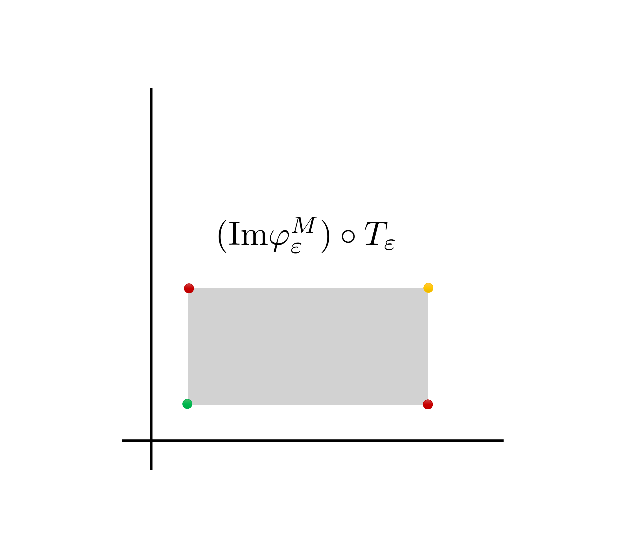
(c) The ε\varepsilon-simplified module Sε​(M)=(Im⁡φεM)∘Tε\textsf{S}_{\varepsilon}(M)=(\Ima\varphi_{\varepsilon}^{M})\circ T_{\varepsilon}.
Figure 7: A 2-parameter interval decomposable module MM under the ε\varepsilon-simplification functor Sε\textsf{S}_{\varepsilon} (3.4).
Definition 3.4 (Simplification Functor).

If M∈𝐯𝐞𝐜𝐭fin𝐑nM\in\mathbf{vect}_{\text{fin}}^{\mathbf{R}^{n}} define the ε\varepsilon-simplification of MM, denoted Sε​(M)\textsf{S}_{\varepsilon}(M), to be the shifted image under the internal translation φεM\varphi_{\varepsilon}^{M} of MM.

Sε​(M)=(Im⁡φεM)∘Tε\textsf{S}_{\varepsilon}(M)=(\Ima\varphi_{\varepsilon}^{M})\circ T_{\varepsilon}
Proposition 3.4 (dI​(M,Sε​(M))≤εd_{I}(M,\textsf{S}_{\varepsilon}(M))\leq\varepsilon).

Sε\textsf{S}_{\varepsilon} is an endofunctor of 𝐕𝐞𝐜𝐭𝐑n\mathbf{Vect}^{\mathbf{R}^{n}} and perturbs modules by no more than ε\varepsilon in the interleaving distance, that is dI​(M,Sε​(M))≤εd_{I}(M,\textsf{S}_{\varepsilon}(M))\leq\varepsilon.

Proof.

The translation functor Tε∗T_{\varepsilon}^{\ast} is clearly a functor and the internal translation is the action of the element 𝐱ε​𝟏∈Pn\mathbf{x}^{\varepsilon\mathbf{1}}\in P_{n} on PnP_{n}-Mod.

We can explicitly define the interleaving morphisms realising dI​(M,Sε​(M))≤εd_{I}(M,\textsf{S}_{\varepsilon}(M))\leq\varepsilon: f:M⇒Sε​(M)∘Tεf:M\Rightarrow\textsf{S}_{\varepsilon}(M)\circ T_{\varepsilon}, g:Sε​(M)⇒M∘Tεg:\textsf{S}_{\varepsilon}(M)\Rightarrow M\circ T_{\varepsilon}. Taking f=φ2​εMf=\varphi_{2\varepsilon}^{M} and g=Im⁡φεM↪M∘Tεg=\Ima\varphi_{\varepsilon}^{M}\hookrightarrow M\circ T_{\varepsilon} we see that Tε∗​(g)∘f=φ2​εMT^{\ast}_{\varepsilon}(g)\circ f=\varphi_{2\varepsilon}^{M} and Tε∗​(f)∘g=φ2​εM∘Tε=φ2​εSε​(M)T^{\ast}_{\varepsilon}(f)\circ g=\varphi_{2\varepsilon}^{M}\circ T_{\varepsilon}=\varphi_{2\varepsilon}^{\textsf{S}_{\varepsilon}(M)}

∎

We explicit the effect of the simplification functor on a multiparameter presentation and on the barcode of a single parameter module.

Lemma 3.1 (Presentation Change under Internal Translation).

Suppose F∙F_{\bullet} is a free resolution of M∈𝐯𝐞𝐜𝐭fin𝐑nM\in\mathbf{vect}_{\text{fin}}^{\mathbf{R}^{n}} and let F1F_{1} and F0F_{0} have generating sets {𝐫i}\{\mathbf{r}_{i}\} and {𝐛j}\{\mathbf{b}_{j}\} respectively. There is a corresponding resolution F∙′F_{\bullet}^{\prime} of Im⁡φεM\Ima\varphi_{\varepsilon}^{M} with a bijective correspondence of generating elements 𝐛∈ξ0​(F0)⟷𝐛′∈ξ0​(F0′)\mathbf{b}\in\xi_{0}(F_{0})\longleftrightarrow\mathbf{b}^{\prime}\in\xi_{0}(F_{0}^{\prime}), 𝐫∈ξ0​(F1)⟷𝐫′∈ξ0​(F1′)\mathbf{r}\in\xi_{0}(F_{1})\longleftrightarrow\mathbf{r}^{\prime}\in\xi_{0}(F_{1}^{\prime}) with the following grading shifts:

gr​(𝐛′)=gr​(𝐛)+ε\text{gr}(\mathbf{b}^{\prime})=\text{gr}(\mathbf{b})+\mathbf{\varepsilon}
gr(𝐫′)=gr(𝐫)∨⋁i:λi≠0gr(𝐛i′) where p1(𝐫)=∑iλi𝐱𝐫−𝐛i⋅𝐛i\text{gr}(\mathbf{r}^{\prime})=\text{gr}(\mathbf{r})\vee\bigvee_{i:\lambda_{i}\neq 0}\text{gr}(\mathbf{b}_{i}^{\prime})\text{ where }p_{1}(\mathbf{r})=\sum_{i}\lambda_{i}\mathbf{x}^{\mathbf{r}-\mathbf{b}_{i}}\cdot\mathbf{b}_{i}

together with the obvious inherited morphisms:

p0′​(𝐛′)=𝐱ε⋅p0​(𝐛)p_{0}^{\prime}(\mathbf{b}^{\prime})=\mathbf{x}^{\mathbf{\varepsilon}}\cdot p_{0}(\mathbf{b})
p1′​(𝐫′)=∑iλi​𝐱𝐫′−𝐛i′⋅𝐛i′p_{1}^{\prime}(\mathbf{r}^{\prime})=\sum_{i}\lambda_{i}\mathbf{x}^{\mathbf{r}^{\prime}-\mathbf{b}^{\prime}_{i}}\cdot\mathbf{b}^{\prime}_{i}
Proof.

Clearly p0′:F0′→Im⁡φεMp_{0}^{\prime}:F_{0}^{\prime}\to\Ima\varphi_{\varepsilon}^{M} is surjective. For every 𝐫′∈ξ0​(F1′)\mathbf{r}^{\prime}\in\xi_{0}(F_{1}^{\prime}) we have that:

p0′∘p1′​(𝐫′)=p0′​(∑iλi​𝐱𝐫′−𝐛i′⋅𝐛i′)=∑iλi​𝐱𝐫′+ε−𝐛i′⋅p0​(𝐛i)=𝐱𝐫′−𝐫⋅∑iλi​𝐱𝐫−𝐛i⋅p0​(𝐛i)=𝐱𝐫′−𝐫⋅p0∘p1​(𝐫)=0p_{0}^{\prime}\circ p_{1}^{\prime}(\mathbf{r}^{\prime})=p_{0}^{\prime}(\sum_{i}\lambda_{i}\mathbf{x}^{\mathbf{r}^{\prime}-\mathbf{b}^{\prime}_{i}}\cdot\mathbf{b}^{\prime}_{i})=\sum_{i}\lambda_{i}\mathbf{x}^{\mathbf{r}^{\prime}+\mathbf{\varepsilon}-\mathbf{b}^{\prime}_{i}}\cdot p_{0}(\mathbf{b}_{i})=\mathbf{x}^{\mathbf{r}^{\prime}-\mathbf{r}}\cdot\sum_{i}\lambda_{i}\mathbf{x}^{\mathbf{r}-\mathbf{b}_{i}}\cdot p_{0}(\mathbf{b}_{i})=\mathbf{x}^{\mathbf{r}^{\prime}-\mathbf{r}}\cdot p_{0}\circ p_{1}(\mathbf{r})=0

and so Im⁡p1′⊂ker⁡p0′\Ima p_{1}^{\prime}\subset\ker p_{0}^{\prime}. Moreover suppose that ∑iλi​𝐱𝐬−𝐛i′⋅𝐛i′∈ker⁡p0′\sum_{i}\lambda_{i}\mathbf{x}^{\mathbf{s}-\mathbf{b}_{i}^{\prime}}\cdot\mathbf{b}_{i}^{\prime}\in\ker p_{0}^{\prime} then ∑iλi​𝐱𝐬+ε−𝐛i⋅𝐛i∈ker⁡p0=Im⁡p1\sum_{i}\lambda_{i}\mathbf{x}^{\mathbf{s}+\mathbf{\varepsilon}-\mathbf{b}_{i}}\cdot\mathbf{b}_{i}\in\ker p_{0}=\Ima p_{1}, hence there exists 𝐫j∈ξ0​(F1)\mathbf{r}_{j}\in\xi_{0}(F_{1}) and scalars μj\mu_{j} such that p1​(∑jμj​𝐱𝐬−𝐫𝐣⋅𝐫j)=∑iλi​𝐱𝐬+ε−𝐛i⋅𝐛ip_{1}(\sum_{j}\mu_{j}\mathbf{x}^{\mathbf{\mathbf{s}-\mathbf{r}_{j}}}\cdot\mathbf{r}_{j})=\sum_{i}\lambda_{i}\mathbf{x}^{\mathbf{s}+\mathbf{\varepsilon}-\mathbf{b}_{i}}\cdot\mathbf{b}_{i} and thus p1′​(∑jμj​𝐱𝐬−𝐫𝐣′⋅𝐫j′)=∑iλi​𝐱𝐬−𝐛i′⋅𝐛i′∈Im⁡p1′p_{1}^{\prime}(\sum_{j}\mu_{j}\mathbf{x}^{\mathbf{\mathbf{s}-\mathbf{r}_{j}^{\prime}}}\cdot\mathbf{r}_{j}^{\prime})=\sum_{i}\lambda_{i}\mathbf{x}^{\mathbf{s}-\mathbf{b}_{i}^{\prime}}\cdot\mathbf{b}_{i}^{\prime}\in\Ima p_{1}^{\prime}. Hence we have shown exactness of F1′→F0′→Im⁡φεM→0F_{1}^{\prime}\to F_{0}^{\prime}\to\Ima\varphi_{\varepsilon}^{M}\to 0. ∎

Lemma 3.2 (Presentation Change under Simplification).

Suppose F∙F_{\bullet} is a free resolution of M∈𝐯𝐞𝐜𝐭fin𝐑nM\in\mathbf{vect}_{\text{fin}}^{\mathbf{R}^{n}} and let F1F_{1} and F0F_{0} have generating sets {𝐫i}\{\mathbf{r}_{i}\} and {𝐛j}\{\mathbf{b}_{j}\} respectively. There is a corresponding resolution F∙′F_{\bullet}^{\prime} of Sε​(M)\textsf{S}_{\varepsilon}(M) with a bijective correspondence of generating elements 𝐛∈ξ0​(F0)⟷𝐛′∈ξ0​(F0′)\mathbf{b}\in\xi_{0}(F_{0})\longleftrightarrow\mathbf{b}^{\prime}\in\xi_{0}(F_{0}^{\prime}), 𝐫∈ξ0​(F1)⟷𝐫′∈ξ0​(F1′)\mathbf{r}\in\xi_{0}(F_{1})\longleftrightarrow\mathbf{r}^{\prime}\in\xi_{0}(F_{1}^{\prime}) with the following grading shifts:

gr​(𝐛′)=gr​(𝐛)\text{gr}(\mathbf{b}^{\prime})=\text{gr}(\mathbf{b})
gr(𝐫′)=(gr(𝐫)∨⋁i:λi≠0gr(𝐛i′))−ε where p1(𝐫)=∑iλi𝐱𝐫−𝐛i⋅𝐛i\text{gr}(\mathbf{r}^{\prime})=\left(\text{gr}(\mathbf{r})\vee\bigvee_{i:\lambda_{i}\neq 0}\text{gr}(\mathbf{b}_{i}^{\prime})\right)-\mathbf{\varepsilon}\text{ where }p_{1}(\mathbf{r})=\sum_{i}\lambda_{i}\mathbf{x}^{\mathbf{r}-\mathbf{b}_{i}}\cdot\mathbf{b}_{i}

together with the obvious inherited morphisms.

Lemma 3.3 (Bar Code Simplification).

Let M∈𝐯𝐞𝐜𝐭𝐑M\in\mathbf{vect}^{\mathbf{R}} have interval decomposition ⨁j∈𝒥𝟙Ij\bigoplus_{j\in\mathcal{J}}\mathds{1}^{I_{j}}, where Ij=[bj,dj)I_{j}=[b_{j},d_{j}). Define the ε\varepsilon-simplification of the intervals IjI_{j} by:

Sε​(Ij)={[bj,∞) if ​dj=∞[bj,dj−ε) if ​dj−bj>ε∅ otherwise.\displaystyle\textsf{S}_{\varepsilon}(I_{j})=\begin{cases}[b_{j},\infty)&\text{ if }d_{j}=\infty\\ [b_{j},d_{j}-\varepsilon)&\text{ if }d_{j}-b_{j}>\varepsilon\\ \emptyset&\text{ otherwise.}\end{cases}

The module Sε​(M)≅⨁j∈𝒥𝟙Sε​(Ij)\textsf{S}_{\varepsilon}(M)\cong\bigoplus_{j\in\mathcal{J}}\mathds{1}^{\textsf{S}_{\varepsilon}(I_{j})}.

Proof.

Consider the minimal free resolution of MM where F0F_{0} is free on the graded set {bj}j∈𝒥\{b_{j}\}_{j\in\mathcal{J}}, F1F_{1} is free on the graded set {dj≠∞}j∈𝒥\{d_{j}\neq\infty\}_{j\in\mathcal{J}}, and p1​(dj)=xdj−bj⋅bjp_{1}(d_{j})=x^{d_{j}-b_{j}}\cdot b_{j}. By 3.1, Sε​(M)\textsf{S}_{\varepsilon}(M) has a corresponding resolution F∙′F_{\bullet}^{\prime}. Moreover F0′F_{0}^{\prime} is free on the graded set {bj′}j∈𝒥\{b_{j}^{\prime}\}_{j\in\mathcal{J}} with grade​(bj′)=bj\text{grade}(b_{j}^{\prime})=b_{j}, F1F_{1} is free on the graded set {dj′}j∈𝒥\{d^{\prime}_{j}\}_{j\in\mathcal{J}} with grade​(dj′)=bj∨(dj−ε)\text{grade}(d_{j}^{\prime})=b_{j}\vee(d_{j}-\varepsilon), and p1′​(dj′)=xdj′−bj′⋅bj′p_{1}^{\prime}(d^{\prime}_{j})=x^{d^{\prime}_{j}-b^{\prime}_{j}}\cdot b^{\prime}_{j}. As claimed, we have coker​(p1′)≅⨁j∈𝒥𝟙Sε​(Ij)\text{coker}(p_{1}^{\prime})\cong\bigoplus_{j\in\mathcal{J}}\mathds{1}^{\textsf{S}_{\varepsilon}(I_{j})}. ∎

The simplification functor naturally restricts to the 1-parameter submodules of a multiparameter persistence modules. For slope 𝟏\mathbf{1} lines ℒ𝐚\mathcal{L}_{\mathbf{a}}, the ε\varepsilon-simplification functor commutes with the restriction to the line ℒ𝐚\mathcal{L}_{\mathbf{a}}:

Sε|ℒ𝐚​(Mℒ𝐚)=Sε​(M)ℒ𝐚\left.\textsf{S}_{\varepsilon}\right|_{\mathcal{L}_{\mathbf{a}}}(M^{\mathcal{L}_{\mathbf{a}}})=\textsf{S}_{\varepsilon}(M)^{\mathcal{L}_{\mathbf{a}}}

Thus using 3.3 we can track how the simplification functor Sε\textsf{S}_{\varepsilon} applied to a multiparameter module affects bar codes in the fibered bar code of that module.

4 Local Equivalence

In this section we prove the main result of this article 4.1.

We make use of the merge and simplification functors defined in Section 3 and their effect on the presentation and fibered bar code of multiparameter persistence modules. After a series of technical lemmas we establish the following local equivalence result:

Theorem 4.1 (Local Equivalence).

Suppose M,N∈𝐯𝐞𝐜𝐭fin𝐑nM,N\in\mathbf{vect}_{\text{fin}}^{\mathbf{R}^{n}} are finitely presented multiparameter persistence modules, and MM has controlling constant cM=c⁡(𝒢M)c_{M}=c(\mathcal{G}_{M}). For all κ∈[0,134)\kappa\in[0,\frac{1}{34}), if dI​(M,N)=εd_{I}(M,N)=\varepsilon and ε<cM2​(34​κ+1)\varepsilon<\frac{c_{M}}{2(34\kappa+1)} then the matching distance is bounded below d0​(M,N)>κ​εd_{0}(M,N)>\kappa\varepsilon.

Let B⁡(M,cM4)⊂(𝐯𝐞𝐜𝐭fin𝐑n,dI)B(M,\frac{c_{M}}{4})\subset(\mathbf{vect}_{\text{fin}}^{\mathbf{R}^{n}},d_{I}) denote the open ball centred at MM of radius cM4\frac{c_{M}}{4}. 4.1 states that for all N∈B⁡(M,cM4)N\in B(M,\frac{c_{M}}{4}) we have:

134​dI​(M,N)≤d0​(M,N)≤dI​(M,N)\frac{1}{34}d_{I}(M,N)\leq d_{0}(M,N)\leq d_{I}(M,N)

In particular, since the interleaving distance is complete on 𝐯𝐞𝐜𝐭fin𝐑n\mathbf{vect}_{\text{fin}}^{\mathbf{R}^{n}}, this result implies that the fibered bar code of MM is distinct from the fibered bar code of any N∈B⁡(M,cM4)N\in B(M,\frac{c_{M}}{4}), and thus is a locally complete invariant for MM.

The proof of 4.1 is built using a series of auxiliary lemmas. The holistic idea for the proof of 4.1 follows the same structure as the proof of the local equivalence result in [CO17]. We assume two modules have a small matching distance in comparison to one of their controlling constants d0​(M,N)=κ​ε≪cMd_{0}(M,N)=\kappa\varepsilon\ll c_{M} and in comparison to their interleaving distance d0​(M,N)=κ​ε≪ε=dI​(M,N)d_{0}(M,N)=\kappa\varepsilon\ll\varepsilon=d_{I}(M,N). We can use the small matching distance d0​(M,N)=κ​ε≪cMd_{0}(M,N)=\kappa\varepsilon\ll c_{M} to deduce that the multiparameter Betti numbers of NN either lie close to the grid Im⁡𝒢M\Ima\mathcal{G}_{M} or can be cancelled with a nearby multiparameter Betti number. Using a series of merges and simplifications we find a nearby module N~\tilde{N}, (dI​(N,N~)≤const⋅κ​εd_{I}(N,\tilde{N})\leq\text{const}\cdot\kappa\varepsilon), such that the multiparameter Betti numbers of N~\tilde{N} are contained in the grid Im⁡𝒢M\Ima\mathcal{G}_{M}. If a δ\delta-interleaving between N~\tilde{N} and MM exist for some δ<cM2\delta<\frac{c_{M}}{2} then 4.9 implies that N~\tilde{N} and MM are isomorphic. We use these results to derive a contradiction to the triangle inequality for the interleaving distance when κ\kappa is too small.

Let us first recall the push function 2.7. Note that the fibre of the push map pushℒ\text{push}_{\mathcal{L}} for an element 𝐚∈ℒ\mathbf{a}\in\mathcal{L} is the boundary of the downset of 𝐚\mathbf{a}:

pushℒ−1​(𝐚)=∂{𝐩∈ℝn:𝐩≤𝐚}\text{push}_{\mathcal{L}}^{-1}(\mathbf{a})=\partial\{\mathbf{p}\in\mathbb{R}^{n}:\mathbf{p}\leq\mathbf{a}\}

Hence for any 𝐩∈ℝn\mathbf{p}\in\mathbb{R}^{n} at least one coordinate of 𝐩\mathbf{p} is preserved by the push function i.e. there is some i∈[n]i\in[n] such that pushℒ​(𝐩)i=pi\text{push}_{\mathcal{L}}(\mathbf{p})_{i}=p_{i}. The push function pushℒ\text{push}_{\mathcal{L}} collapses ℝn\mathbb{R}^{n} to the line ℒ\mathcal{L} whilst preserving the partial order. Thus given a resolution of a multiparameter module MM the push function induces a resolution of MℒM^{\mathcal{L}}.

Lemma 4.1 (Induced 1-Parameter Resolution).

Let ℒ:ℝ→ℝn\mathcal{L}:\mathbb{R}\to\mathbb{R}^{n} be a positively sloped line and suppose M∈𝐕𝐞𝐜𝐭𝐑nM\in\mathbf{Vect}^{\mathbf{R}^{n}} has a free resolution F∙→MF_{\bullet}\to M. The 11-parameter submodule Mℒ:=M∘ℒ∈𝐕𝐞𝐜𝐭𝐑M^{\mathcal{L}}:=M\circ\mathcal{L}\in\mathbf{Vect}^{\mathbf{R}} has a corresponding free resolution F∙ℒF_{\bullet}^{\mathcal{L}}, where the generators of FiF_{i} are in bijection with the generators of FiℒF_{i}^{\mathcal{L}}; in particular a generator 𝐚\mathbf{a} of FiF_{i} corresponds to a generator 𝐚ℒ\mathbf{a}^{\mathcal{L}} of FiℒF_{i}^{\mathcal{L}} with ℝ\mathbb{R}-grading given by ℒ−1∘pushℒ​(𝐚)\mathcal{L}^{-1}\circ\text{push}_{\mathcal{L}}(\mathbf{a}).

Proof.

It is straightforward to check that the pullback functor ℒ∗:𝐕𝐞𝐜𝐭𝐑n→𝐕𝐞𝐜𝐭𝐑\mathcal{L}^{\ast}:\mathbf{Vect}^{\mathbf{R}^{n}}\to\mathbf{Vect}^{\mathbf{R}} preserves free modules, and preserves exactness since exactness of a sequence of persistence modules may be checked pointwise. ∎

Let M∈𝐯𝐞𝐜𝐭𝐑M\in\mathbf{vect}^{\mathbf{R}} with free resolution F∙→MF_{\bullet}\to M. The decomposition theorem of [CB14], gives rise to an isomorphism ϕ:M→⨁j∈𝒥𝟙Ij\phi:M\to\bigoplus_{j\in\mathcal{J}}\mathds{1}^{I_{j}} for some indexed set of intervals {Ij=[bj,dj)}j∈𝒥\{I_{j}=[b_{j},d_{j})\}_{j\in\mathcal{J}}. For the purposes of this paper we shall require that |J|=|ξ0​(F0)||J|=|\xi_{0}(F_{0})| and hence allow for IjI_{j} to be empty intervals. Let F∙′F^{\prime}_{\bullet} denote the free resolution of ⨁j∈𝒥𝟙Ij\bigoplus_{j\in\mathcal{J}}\mathds{1}^{I_{j}}, where F0′=Free​[{bj}j∈𝒥]F^{\prime}_{0}=\text{Free}[\{b_{j}\}_{j\in\mathcal{J}}], F1′=Free[{dj≠∞}j∈𝒥]F^{\prime}_{1}=\text{Free}[\{d_{j}\neq\infty\}_{j\in\mathcal{J}}] and dj↦xdj−bj⋅bjd_{j}\mapsto x^{d_{j}-b_{j}}\cdot b_{j}. We shall refer to F∙′F^{\prime}_{\bullet} as the canonical free resolution of ⨁j∈𝒥𝟙Ij\bigoplus_{j\in\mathcal{J}}\mathds{1}^{I_{j}}.

Again let ⟨⋅,⋅⟩\langle\cdot,\cdot\rangle denote the point-wise vector space inner product of a free module for which makes the generating set an orthonormal basis at each grade. Note that the isomorphism ϕ\phi gives rise to a chain map ϕ∙:F∙→F∙′\phi_{\bullet}:F_{\bullet}\to F^{\prime}_{\bullet}.

Definition 4.1 (Bars generated by 𝐛\mathbf{b} and killed by 𝐫\mathbf{r}).

For a fixed isomorphism ϕ\phi and resolution F∙F_{\bullet} we say that (a generator of F0F_{0}) b{b} generates the bar IjI_{j} if gr​(b)=gr​(bj)\text{gr}(b)=\text{gr}(b_{j}) and ⟨ϕ0​(b),bj⟩≠0\langle\phi_{0}({b}),b_{j}\rangle\neq 0. Moreover we say that (a generator of F1F_{1}) r{r} kills the bar IjI_{j} if gr​(r)=gr​(rj)\text{gr}(r)=\text{gr}(r_{j}) and ⟨ϕ1​(r),rj⟩≠0\langle\phi_{1}({r}),{r_{j}}\rangle\neq 0.

For M∈𝐯𝐞𝐜𝐭fin𝐑nM\in\mathbf{vect}_{\text{fin}}^{\mathbf{R}^{n}} with free resolution F∙→MF_{\bullet}\to M recall there is a corresponding free resolution F∙ℒF^{\mathcal{L}}_{\bullet} of MℒM^{\mathcal{L}}. Given fixed decomposition isomorphisms ϕℒ:Mℒ→⨁j∈𝒥ℒ𝟙Ij\phi_{\mathcal{L}}:M^{\mathcal{L}}\to\bigoplus_{j\in\mathcal{J}_{\mathcal{L}}}\mathds{1}^{I_{j}} for all positively sloped lines ℒ\mathcal{L}, we say that 𝐛\mathbf{b} (a generator of F0F_{0}) generates the bar IjI_{j} in MℒM^{\mathcal{L}} if 𝐛ℒ\mathbf{b}^{\mathcal{L}} generates IjI_{j} in MℒM^{\mathcal{L}}. Similarly we say that the relation 𝐫\mathbf{r} (a generator of F1F_{1}) kills the bar IjI_{j}, if 𝐫ℒ\mathbf{r}^{\mathcal{L}} kills the bar IjI_{j} in MℒM^{\mathcal{L}}.

Remark 4.1.

We can fix isomorphisms ϕℒ\phi_{\mathcal{L}} such that each bar in MℒM^{\mathcal{L}} is generated by a unique b∈ξ0​(F0ℒ){b}\in\xi_{0}(F_{0}^{\mathcal{L}}) and killed by a unique r∈ξ0​(F1ℒ){r}\in\xi_{0}(F_{1}^{\mathcal{L}}). Moreover we can ensure every generator b∈ξ0​(F0ℒ){b}\in\xi_{0}(F_{0}^{\mathcal{L}}) generates some bar in MℒM^{\mathcal{L}} (albeit these bars may be of zero length). See for example the reduction algorithm of [EH10]. We shall fix our decomposition isomorphisms to have this property.

Our next lemma identifies the fibre of the push map.

Lemma 4.2 (Fibre of the Push Map).

Suppose 𝐚=(a1,…,an)\mathbf{a}=(a_{1},...,a_{n}), 𝐛=(b1,…,bn)\mathbf{b}=(b_{1},...,b_{n}) are such that ‖pushℒ𝐛​(𝐚)−𝐛‖∞≤δ\|\text{push}_{\mathcal{L}_{\mathbf{b}}}(\mathbf{a})-\mathbf{b}\|_{\infty}\leq\delta then mini∈[n]⁡|ai−bi|≤δ\min_{i\in[n]}|a_{i}-b_{i}|\leq\delta. In particular, if 𝐚∈Im⁡𝒢\mathbf{a}\in\Ima\mathcal{G} then 𝐛\mathbf{b} is δ\delta-close to Grid𝒢\text{Grid}_{\mathcal{G}}.

Proof.

At least one of the coordinates aia_{i} is preserved by the push map. ∎

Suppose modules MM and NN satisfy the assumptions of 4.1. 4.2 will be used to identify that the multiparameter Betti numbers inducing births of long bars in the fibered bar code of NN must lie close to the grid of MM.

In 4.6 we use the positions of births of bars in the fibered bar code of MM to limit the positions of generators of NN. 4.3 establishes that every non trivial generator of NN generates some non-empty bar in the fibered bar code of NN.

Lemma 4.3 (Non-trivial Generators Generate Non-zero Bars).

Let M∈𝐯𝐞𝐜𝐭fin𝐑nM\in\mathbf{vect}_{\text{fin}}^{\mathbf{R}^{n}} be a finitely presented multiparameter persistence module. If 𝐛∈ξ0​(M)\mathbf{b}\in\xi_{0}(M) then 𝐛\mathbf{b} generates a non-trivial bar in Mℒ𝐛M^{\mathcal{L}_{\mathbf{b}}}.

Proof.

Suppose that MM has minimal free resolution (F∙,p∙)(F_{\bullet},p_{\bullet}), decomposition isomorphism ϕ:Mℒ𝐛​→~​⨁j∈𝒥ℒ𝟙Ij\phi:M^{\mathcal{L}_{\mathbf{b}}}\tilde{\to}\bigoplus_{j\in\mathcal{J}_{\mathcal{L}}}\mathds{1}^{I_{j}}, and ⨁j∈𝒥ℒ𝟙Ij\bigoplus_{j\in\mathcal{J}_{\mathcal{L}}}\mathds{1}^{I_{j}} has canonical free resolution (F∙′,p∙′)(F_{\bullet}^{\prime},p_{\bullet}^{\prime}). Suppose that ϕ0​(𝐛ℒ𝐛)=bj\phi_{0}(\mathbf{b}^{\mathcal{L}_{\mathbf{b}}})=b_{j} and Ij=∅I_{j}=\emptyset. By the exactness of the resolution (F∙ℒ𝐛,p∙ℒ𝐛)(F_{\bullet}^{\mathcal{L}_{\mathbf{b}}},p_{\bullet}^{\mathcal{L}_{\mathbf{b}}}) there is some 𝐫∈ξ1​(M)\mathbf{r}\in\xi_{1}(M) such that ϕ1​(𝐫ℒ𝐛)=rj\phi_{1}(\mathbf{r}^{\mathcal{L}_{\mathbf{b}}})=r_{j} and gr​(𝐛ℒ𝐛)=gr​(𝐫ℒ𝐛)\text{gr}(\mathbf{b}^{\mathcal{L}_{\mathbf{b}}})=\text{gr}(\mathbf{r}^{\mathcal{L}_{\mathbf{b}}}). The fact that ϕ1​(𝐫ℒ𝐛)=rj\phi_{1}(\mathbf{r}^{\mathcal{L}_{\mathbf{b}}})=r_{j} implies that ⟨p1​(𝐫),𝐛⟩≠0\langle p_{1}(\mathbf{r}),\mathbf{b}\rangle\neq 0. Moreover ⟨p1​(𝐫),𝐛⟩≠0\langle p_{1}(\mathbf{r}),\mathbf{b}\rangle\neq 0 implies that gr​(𝐫)≥gr​(𝐛)\text{gr}(\mathbf{r})\geq\text{gr}(\mathbf{b}). Together gr​(𝐫)≥gr​(𝐛)\text{gr}(\mathbf{r})\geq\text{gr}(\mathbf{b}) and gr​(𝐛ℒ𝐛)=gr​(𝐫ℒ𝐛)\text{gr}(\mathbf{b}^{\mathcal{L}_{\mathbf{b}}})=\text{gr}(\mathbf{r}^{\mathcal{L}_{\mathbf{b}}}) imply that gr​(𝐫)=gr​(𝐛)\text{gr}(\mathbf{r})=\text{gr}(\mathbf{b}). Thus 𝐛\mathbf{b} and 𝐫\mathbf{r} satisfy the hypotheses of 2.2 and are a cancellation pair, contradicting the minimality of (F∙,p∙)(F_{\bullet},p_{\bullet}).

∎

Similarly, in 4.7 we use the positions of deaths of bars in the fibered bar code of MM to determine the positions of relations of NN. 4.4 establishes that every non trivial relation of NN kill some non-empty bar in the fibered bar code of NN.

Lemma 4.4 (Non-trivial Relations Kill).

Let M∈𝐯𝐞𝐜𝐭fin𝐑nM\in\mathbf{vect}_{\text{fin}}^{\mathbf{R}^{n}} be a finitely presented multiparameter persistence module. If 𝐫∈ξ1​(M)\mathbf{r}\in\xi_{1}(M) then 𝐫ℒ𝐫∉ker⁡p1ℒ𝐫\mathbf{r}^{\mathcal{L}_{\mathbf{r}}}\notin\ker p_{1}^{\mathcal{L}_{\mathbf{r}}} and so 𝐫\mathbf{r} kills a bar in Mℒ𝐫≅⨁j∈𝒥ℒϕ⁡𝟙IjM^{\mathcal{L}_{\mathbf{r}}}\cong_{\phi}\bigoplus_{j\in\mathcal{J}_{\mathcal{L}}}\mathds{1}^{I_{j}}.

Proof.

Suppose that MM has minimal free resolution (F∙,p∙)(F_{\bullet},p_{\bullet}), decomposition isomorphism ϕ:Mℒ𝐫​→~​⨁j∈𝒥ℒ𝟙Ij\phi:M^{\mathcal{L}_{\mathbf{r}}}\tilde{\to}\bigoplus_{j\in\mathcal{J}_{\mathcal{L}}}\mathds{1}^{I_{j}}, and ⨁j∈𝒥ℒ𝟙Ij\bigoplus_{j\in\mathcal{J}_{\mathcal{L}}}\mathds{1}^{I_{j}} has canonical free resolution (F∙′,p∙′)(F_{\bullet}^{\prime},p_{\bullet}^{\prime}). If 𝐫ℒ𝐫∈ker⁡p1ℒ𝐫\mathbf{r}^{\mathcal{L}_{\mathbf{r}}}\in\ker p_{1}^{\mathcal{L}_{\mathbf{r}}} then by exactness of the resolution (F∙ℒ𝐫,p∙ℒ𝐫)(F_{\bullet}^{\mathcal{L}_{\mathbf{r}}},p_{\bullet}^{\mathcal{L}_{\mathbf{r}}}) there is some 𝐬∈ξ2​(M)\mathbf{s}\in\xi_{2}(M) such that ⟨p2ℒ𝐫​(𝐬ℒ𝐫),𝐫ℒ𝐫⟩≠0\langle p_{2}^{\mathcal{L}_{\mathbf{r}}}(\mathbf{s}^{\mathcal{L}_{\mathbf{r}}}),\mathbf{r}^{\mathcal{L}_{\mathbf{r}}}\rangle\neq 0 and gr​(𝐫ℒ𝐫)=gr​(𝐬ℒ𝐫)\text{gr}(\mathbf{r}^{\mathcal{L}_{\mathbf{r}}})=\text{gr}(\mathbf{s}^{\mathcal{L}_{\mathbf{r}}}). The fact that ⟨p2ℒ𝐫​(𝐬ℒ𝐫),𝐫ℒ𝐫⟩≠0\langle p_{2}^{\mathcal{L}_{\mathbf{r}}}(\mathbf{s}^{\mathcal{L}_{\mathbf{r}}}),\mathbf{r}^{\mathcal{L}_{\mathbf{r}}}\rangle\neq 0 implies that gr​(𝐬)≥gr​(𝐫)\text{gr}(\mathbf{s})\geq\text{gr}(\mathbf{r}). Together gr​(𝐬)≥gr​(𝐫)\text{gr}(\mathbf{s})\geq\text{gr}(\mathbf{r}) and gr​(𝐫ℒ𝐫)=gr​(𝐬ℒ𝐫)\text{gr}(\mathbf{r}^{\mathcal{L}_{\mathbf{r}}})=\text{gr}(\mathbf{s}^{\mathcal{L}_{\mathbf{r}}}) imply that gr​(𝐬)=gr​(𝐫)\text{gr}(\mathbf{s})=\text{gr}(\mathbf{r}). Thus 𝐫\mathbf{r} and 𝐬\mathbf{s} satisfy the hypotheses of 2.2 and are a cancellation pair, contradicting the minimality of (F∙,p∙)(F_{\bullet},p_{\bullet}). Suppose that 𝐫\mathbf{r} does not kill a bar and so ϕ1​(𝐫ℒ𝐫)=0\phi_{1}(\mathbf{r}^{\mathcal{L}_{\mathbf{r}}})=0. Since (F∙′,p∙′)(F_{\bullet}^{\prime},p_{\bullet}^{\prime}) is the canonical free resolution ϕ0\phi_{0} is an isomorphism, and so ϕ1​(𝐫ℒ𝐫)=0\phi_{1}(\mathbf{r}^{\mathcal{L}_{\mathbf{r}}})=0 implies that 𝐫ℒ𝐫∈ker⁡p1\mathbf{r}^{\mathcal{L}_{\mathbf{r}}}\in\ker p_{1}. Thus it must be that 𝐫\mathbf{r} kills a bar in Mℒ𝐫≅⨁j∈𝒥ℒϕ⁡𝟙IjM^{\mathcal{L}_{\mathbf{r}}}\cong_{\phi}\bigoplus_{j\in\mathcal{J}_{\mathcal{L}}}\mathds{1}^{I_{j}}.

∎

Through the proof of 4.4, we observe that a relation 𝐫∈ξ1​(M)\mathbf{r}\in\xi_{1}(M)which does not kill a bar must instead be lie in the image of a second order relation 𝐬∈ξ2​(M)\mathbf{s}\in\xi_{2}(M).

Definition 4.2 (Unmerge Function).

Let 𝒢=Π​𝒢i\mathcal{G}=\Pi\mathcal{G}^{i} be a grid with δ<c⁡(𝒢)2\delta<\frac{c(\mathcal{G})}{2}, and let 𝐞i\mathbf{e}_{i} denote the standard basis vector of ℝn\mathbb{R}^{n}. The unmerge function Uδ𝒢\textsf{U}_{\delta}^{\mathcal{G}} maps points lying on Grid𝒢\text{Grid}_{\mathcal{G}} to lie δ\delta far away from the grid: Uδ𝒢:Grid𝒢→ℝn\textsf{U}_{\delta}^{\mathcal{G}}:\text{Grid}_{\mathcal{G}}\to\mathbb{R}^{n}. For 𝐚∈Grid𝒢\mathbf{a}\in\text{Grid}_{\mathcal{G}} let ℐ𝐚\mathcal{I}_{\mathbf{a}} be the indices of the coordinates of 𝐚\mathbf{a} such that |ai−Im⁡𝒢i|≤δ|a_{i}-\Ima\mathcal{G}^{i}|\leq\delta. We define the δ\delta-unmerge of 𝐚\mathbf{a} as follows:

Uδ𝒢​(𝐚)=Mδ𝒢​(𝐚)+δ​∑i∈ℐ𝐚𝐞i\textsf{U}_{\delta}^{\mathcal{G}}(\mathbf{a})=\textsf{M}_{\delta}^{\mathcal{G}}(\mathbf{a})+\delta\sum_{i\in\mathcal{I}_{\mathbf{a}}}\mathbf{e}_{i}

By construction the unmerge function takes 𝐚\mathbf{a} and returns the maximum element in the poset ℝn\mathbb{R}^{n} which merges to same point as 𝐚\mathbf{a} that is:

Uδ𝒢​(𝐚)=max⁡{𝐩∈ℝn:Mδ𝒢​(𝐩)=Mδ𝒢​(𝐚)}\textsf{U}_{\delta}^{\mathcal{G}}(\mathbf{a})=\max\{\mathbf{p}\in\mathbb{R}^{n}:\textsf{M}_{\delta}^{\mathcal{G}}(\mathbf{p})=\textsf{M}_{\delta}^{\mathcal{G}}(\mathbf{a})\}

Thus for all 𝐚∈Grid𝒢\mathbf{a}\in\text{Grid}_{\mathcal{G}} we have ‖Uδ𝒢​(𝐚)−Grid𝒢‖∞=δ\|\textsf{U}_{\delta}^{\mathcal{G}}(\mathbf{a})-\text{Grid}_{\mathcal{G}}\|_{\infty}=\delta. See Figure 8 for examples of the unmerge function.

Refer to caption
(a) Uδ𝒢\textsf{U}_{\delta}^{\mathcal{G}} applied to points 𝐩,𝐪∈ℝ2\mathbf{p},\mathbf{q}\in\mathbb{R}^{2}.
Refer to caption
(b) Uδ𝒢\textsf{U}_{\delta}^{\mathcal{G}} applied to points 𝐩,𝐪,𝐬∈ℝ3\mathbf{p},\mathbf{q},\mathbf{s}\in\mathbb{R}^{3}.
Figure 8: Examples of the unmerge function Uδ𝒢\textsf{U}_{\delta}^{\mathcal{G}} moving points from Grid𝒢\text{Grid}_{\mathcal{G}} to lie δ\delta-far away from Grid𝒢\text{Grid}_{\mathcal{G}}.

The following result, 4.5, will be used to show that the grades of multiparameter Betti numbers of NN merge to the same grade and satisfy the hypotheses of 2.2 and thus cancel each other out.

Lemma 4.5 (Sufficient Conditions for Grades to Merge).

Let 𝐚,𝐛∈(𝐑n,≤)\mathbf{a},\mathbf{b}\in(\mathbf{R}^{n},\leq) and 𝒢\mathcal{G} be a grid function such that: ‖𝐚−Grid𝒢‖∞≤δ\|\mathbf{a}-\text{Grid}_{\mathcal{G}}\|_{\infty}\leq\delta and 𝐛≥𝐚\mathbf{b}\geq\mathbf{a}. If pushℒUδ𝒢​Mδ𝒢​(𝐚)​(𝐚)=pushℒUδ𝒢​Mδ𝒢​(𝐚)​(𝐛)\text{push}_{\mathcal{L}_{\textsf{U}_{\delta}^{\mathcal{G}}\textsf{M}_{\delta}^{\mathcal{G}}({\mathbf{a}})}}({\mathbf{a}})=\text{push}_{\mathcal{L}_{\textsf{U}_{\delta}^{\mathcal{G}}\textsf{M}_{\delta}^{\mathcal{G}}({\mathbf{a}})}}({\mathbf{b}}), then Mδ𝒢​(𝐚)=Mδ𝒢​(𝐛)\textsf{M}_{\delta}^{\mathcal{G}}({\mathbf{a}})=\textsf{M}_{\delta}^{\mathcal{G}}({\mathbf{b}}).

Proof.

Since pushℒUδ𝒢​Mδ𝒢​(𝐚)​(𝐚)=pushℒUδ𝒢​Mδ𝒢​(𝐚)​(𝐛)\text{push}_{\mathcal{L}_{\textsf{U}_{\delta}^{\mathcal{G}}\textsf{M}_{\delta}^{\mathcal{G}}({\mathbf{a}})}}({\mathbf{a}})=\text{push}_{\mathcal{L}_{\textsf{U}_{\delta}^{\mathcal{G}}\textsf{M}_{\delta}^{\mathcal{G}}({\mathbf{a}})}}({\mathbf{b}}) and 𝐛≥𝐚\mathbf{b}\geq\mathbf{a}, then 𝐛∈pushℒUδ𝒢​Mδ𝒢​(𝐚)−1(0)∩{≥𝐚}=[𝐚,Uδ𝒢Mδ𝒢(𝐚)]\mathbf{b}\in\text{push}^{-1}_{\mathcal{L}_{\textsf{U}_{\delta}^{\mathcal{G}}\textsf{M}_{\delta}^{\mathcal{G}}({\mathbf{a}})}}(0)\cap\{\geq\mathbf{a}\}=[\mathbf{a},\textsf{U}_{\delta}^{\mathcal{G}}\textsf{M}_{\delta}^{\mathcal{G}}({\mathbf{a}})], where [𝐚,Uδ𝒢​Mδ𝒢​(𝐚)][\mathbf{a},\textsf{U}_{\delta}^{\mathcal{G}}\textsf{M}_{\delta}^{\mathcal{G}}({\mathbf{a}})] denotes the interval between 𝐚\mathbf{a} and Uδ𝒢​Mδ𝒢​(𝐚)\textsf{U}_{\delta}^{\mathcal{G}}\textsf{M}_{\delta}^{\mathcal{G}}({\mathbf{a}}). By definition of the unmerge function, the coordinate values of 𝐚\mathbf{a} which are unchanged by Mδ𝒢\textsf{M}_{\delta}^{\mathcal{G}} are also unchanged when applying Uδ𝒢\textsf{U}_{\delta}^{\mathcal{G}} to Mδ𝒢​(𝐚)\textsf{M}_{\delta}^{\mathcal{G}}(\mathbf{a}). Thus 𝐚\mathbf{a} and 𝐛\mathbf{b} share coordinate values for all the coordinate values of 𝐚\mathbf{a} which are unchanged by Mδ𝒢\textsf{M}_{\delta}^{\mathcal{G}}. Since ‖Uδ𝒢​Mδ𝒢​(𝐚)−Grid𝒢‖∞=δ\|\textsf{U}_{\delta}^{\mathcal{G}}\textsf{M}_{\delta}^{\mathcal{G}}(\mathbf{a})-\text{Grid}_{\mathcal{G}}\|_{\infty}=\delta, then ‖𝐛−Grid𝒢‖∞≤δ\|\mathbf{b}-\text{Grid}_{\mathcal{G}}\|_{\infty}\leq\delta, and so the remaining coordinates of 𝐛\mathbf{b} are merged to the same coordinate values of Mδ𝒢​(𝐚)\textsf{M}_{\delta}^{\mathcal{G}}(\mathbf{a}), thus it follows that Mδ𝒢​(𝐚)=Mδ𝒢​(𝐛)\textsf{M}_{\delta}^{\mathcal{G}}({\mathbf{a}})=\textsf{M}_{\delta}^{\mathcal{G}}({\mathbf{b}}). ∎

4.6 and 4.7 use the small matching distance to derive properties about the gradings of the generators and relations of NN and the length of the bars the generators and relations birth and kill in the fibered bar code.

Lemma 4.6 (Properties of Generators).

Suppose d0​(M,N)<κ​εd_{0}(M,N)<\kappa\varepsilon and cM>2​κ​εc_{M}>2\kappa\varepsilon. For all 𝐛∈ξ0​(N)\mathbf{b}\in\xi_{0}(N), at least one of the following properties holds:

  1. B.1

    𝐛\mathbf{b} lies 2​κ​ε2\kappa\varepsilon-close to Im⁡𝒢M\Ima\mathcal{G}_{M}

  2. B.2

    𝐛\mathbf{b} lies κ​ε\kappa\varepsilon-close to Grid𝒢M\text{Grid}_{\mathcal{G}_{M}} and generates a bar of length less than 2​κ​ε2\kappa\varepsilon in the module NℒUκ​ϵ𝒢M​Mκ​ε𝒢M​(𝐛)N^{\mathcal{L}_{\textsf{U}_{\kappa\epsilon}^{\mathcal{G}_{M}}\textsf{M}^{\mathcal{G}_{M}}_{\kappa\varepsilon}(\mathbf{b})}}

  3. B.3

    𝐛\mathbf{b} generates a bar of length less than 2​κ​ε2\kappa\varepsilon in the module Nℒ𝐛N^{\mathcal{L}_{\mathbf{b}}}

Proof.

Consider the module Nℒ𝐛N^{\mathcal{L}_{\mathbf{b}}}. Since 𝐛∈ξ0​(N)\mathbf{b}\in\xi_{0}(N) is a non-trivial generator, 𝐛\mathbf{b} generates a non-trivial bar in Nℒ𝐛N^{\mathcal{L}_{\mathbf{b}}} (4.3). Suppose the bar in Nℒ𝐛N^{\mathcal{L}_{\mathbf{b}}} generated by 𝐛\mathbf{b} has length <2​κ​ε<2\kappa\varepsilon, then we satisfy property B.3.

Else the bar generated by 𝐛\mathbf{b} in Nℒ𝐛N^{\mathcal{L}_{\mathbf{b}}} has length ≥2​κ​ε\geq 2\kappa\varepsilon and must be κ​ε\kappa\varepsilon-matched with a bar in the module Mℒ𝐛M^{\mathcal{L}_{\mathbf{b}}}. Hence by 4.2, 𝐛\mathbf{b} is κ​ε\kappa\varepsilon-close to Grid𝒢M\text{Grid}_{\mathcal{G}_{M}}. If 𝐛\mathbf{b} is 2​κ​ε2\kappa\varepsilon-close to Im⁡𝒢M\Ima\mathcal{G}_{M} we satisfy B.1, else 𝐛\mathbf{b} is >2​κ​ε>2\kappa\varepsilon from all grid points of MM.

Mκ​ε𝒢M​(𝐛)\textsf{M}_{\kappa\varepsilon}^{\mathcal{G}_{M}}(\mathbf{b}) lies on Grid𝒢M\text{Grid}_{\mathcal{G}_{M}} but is not in the image of 𝒢M\mathcal{G}_{M}. Using the fact that cM>2​κ​εc_{M}>2\kappa\varepsilon and at least one of the coordinates of 𝐛\mathbf{b} is unchanged by Mκ​ε𝒢M\textsf{M}_{\kappa\varepsilon}^{\mathcal{G}_{M}}, we have that the κ​ε\kappa\varepsilon-close line ℒUκ​ε𝒢M​Mκ​ε𝒢M​(𝐛)\mathcal{L}_{\textsf{U}_{\kappa\varepsilon}^{\mathcal{G}_{M}}\textsf{M}_{\kappa\varepsilon}^{\mathcal{G}_{M}}(\mathbf{b})} is such that ‖pushℒUκ​ε𝒢M​Mκ​ε𝒢M​(𝐛)​(𝐛)−pushℒUκ​ε𝒢M​Mκ​ε𝒢M​(𝐛)​(𝒢M)‖∞=κ​ε\|\text{push}_{\mathcal{L}_{\textsf{U}_{\kappa\varepsilon}^{\mathcal{G}_{M}}\textsf{M}_{\kappa\varepsilon}^{\mathcal{G}_{M}}(\mathbf{b})}}(\mathbf{b})-\text{push}_{\mathcal{L}_{\textsf{U}_{\kappa\varepsilon}^{\mathcal{G}_{M}}\textsf{M}_{\kappa\varepsilon}^{\mathcal{G}_{M}}(\mathbf{b})}}(\mathcal{G}_{M})\|_{\infty}=\kappa\varepsilon. Since pushℒUκ​ε𝒢M​Mκ​ε𝒢M​(𝐛)​(Mκ​ε𝒢M​(𝐛))\text{push}_{\mathcal{L}_{\textsf{U}_{\kappa\varepsilon}^{\mathcal{G}_{M}}\textsf{M}_{\kappa\varepsilon}^{\mathcal{G}_{M}}(\mathbf{b})}}(\textsf{M}_{\kappa\varepsilon}^{\mathcal{G}_{M}}(\mathbf{b})) is κ​ε\kappa\varepsilon far from all points of pushℒUκ​ε𝒢M​Mκ​ε𝒢M​(𝐛)​(𝒢M)\text{push}_{\mathcal{L}_{\textsf{U}_{\kappa\varepsilon}^{\mathcal{G}_{M}}\textsf{M}_{\kappa\varepsilon}^{\mathcal{G}_{M}}(\mathbf{b})}}(\mathcal{G}_{M}) and d0​(M,N)<κ​εd_{0}(M,N)<\kappa\varepsilon, then the bar generated by 𝐛\mathbf{b} in NℒUκ​ε𝒢M​Mκ​ε𝒢M​(𝐛){N}^{\mathcal{L}_{\textsf{U}_{\kappa\varepsilon}^{\mathcal{G}_{M}}\textsf{M}_{\kappa\varepsilon}^{\mathcal{G}_{M}}(\mathbf{b})}} cannot be matched to bars in MℒUκ​ε𝒢M​Mκ​ε𝒢M​(𝐛)M^{\mathcal{L}_{\textsf{U}_{\kappa\varepsilon}^{\mathcal{G}_{M}}\textsf{M}_{\kappa\varepsilon}^{\mathcal{G}_{M}}(\mathbf{b})}} and so must be length <2​κ​ϵ<2\kappa\epsilon. ∎

Lemma 4.7 (Properties of Relations).

Suppose d0​(M,N)<κ​εd_{0}(M,N)<\kappa\varepsilon, ξ0​(N)⊂Im⁡𝒢M\xi_{0}(N)\subset\Ima\mathcal{G}_{M} and that cM>4​κ​ϵc_{M}>4\kappa\epsilon. For all 𝐫∈ξ1​(N)\mathbf{r}\in\xi_{1}(N), one of the following properties holds:

  1. R.1

    𝐫\mathbf{r} is 2​κ​ε2\kappa\varepsilon-close to Im⁡𝒢M\Ima\mathcal{G}_{M}

  2. R.2

    𝐫\mathbf{r} is 2​κ​ε2\kappa\varepsilon-close to Grid𝒢M\text{Grid}_{\mathcal{G}_{M}} and for all α∈(0,cM−4​κ​ε2)\alpha\in(0,\frac{c_{M}-4\kappa\varepsilon}{2}) if it kills a bar in the module NℒU2​κ​ε+α𝒢M​M2​κ​ε𝒢M​(𝐫)N^{\mathcal{L}_{\textsf{U}_{2\kappa\varepsilon+\alpha}^{\mathcal{G}_{M}}\textsf{M}_{2\kappa\varepsilon}^{\mathcal{G}_{M}}(\mathbf{r})}} that bar is of length less than 2​κ​ε2\kappa\varepsilon

Proof.

For each 𝐫∈ξ1​(N){\mathbf{r}}\in\xi_{1}({N}) consider the bar killed by 𝐫{\mathbf{r}} in the module Nℒ𝐫{N}^{\mathcal{L}_{{\mathbf{r}}}} (4.4). Since dI​(M,N)<κ​ϵd_{I}(M,{N})<\kappa\epsilon the bar killed by 𝐫{\mathbf{r}} is either κ​ε\kappa\varepsilon-matched to a bar of Mℒ𝐫M^{\mathcal{L}_{{\mathbf{r}}}} and thus 𝐫\mathbf{r} is κ​ε\kappa\varepsilon-close to Grid𝒢M\text{Grid}_{\mathcal{G}_{M}} (by 4.2), else the bar is 2​κ​ε2\kappa\varepsilon-trivial and unmatched – in which case it is 2​κ​ε2\kappa\varepsilon-close to a coordinate of a generator of NN and since ξ0​(N)⊂Im⁡𝒢M\xi_{0}(N)\subset\Ima\mathcal{G}_{M} then 𝐫\mathbf{r} is 2​κ​ε2\kappa\varepsilon-close to Grid𝒢M\text{Grid}_{\mathcal{G}_{M}}. In either case 𝐫{\mathbf{r}} is 2​κ​ε2\kappa\varepsilon-close to Grid𝒢M\text{Grid}_{\mathcal{G}_{M}}.

If ‖𝐫−Im⁡𝒢M‖∞>2​κ​ε\|{\mathbf{r}}-\Ima\mathcal{G}_{M}\|_{\infty}>2\kappa\varepsilon then at least one of the coordinates of 𝐫\mathbf{r} is unchanged by M2​κ​ε𝒢M\textsf{M}_{2\kappa\varepsilon}^{\mathcal{G}_{M}} and so we yield that:

‖pushℒU2​κ​ε+α𝒢M​M2​κ​ε𝒢M​(𝐫)​(𝐫)−pushℒU2​κ​ε+α𝒢M​M2​κ​ε𝒢M​(𝐫)​(Im⁡𝒢M)‖∞=2​κ​ε+α\|\text{push}_{\mathcal{L}_{\textsf{U}_{2\kappa\varepsilon+\alpha}^{\mathcal{G}_{M}}\textsf{M}_{2\kappa\varepsilon}^{\mathcal{G}_{M}}({\mathbf{r}})}}(\mathbf{r})-\text{push}_{\mathcal{L}_{\textsf{U}_{2\kappa\varepsilon+\alpha}^{\mathcal{G}_{M}}\textsf{M}_{2\kappa\varepsilon}^{\mathcal{G}_{M}}({\mathbf{r}})}}(\Ima\mathcal{G}_{M})\|_{\infty}=2\kappa\varepsilon+\alpha

Hence any bar killed by 𝐫\mathbf{r} in the module NℒU2​κ​ε𝒢M​M2​κ​ε𝒢M​(𝐫)N^{\mathcal{L}_{\textsf{U}_{2\kappa\varepsilon}^{\mathcal{G}_{M}}\textsf{M}_{2\kappa\varepsilon}^{\mathcal{G}_{M}}(\mathbf{r})}} is unmatched and so of length less than 2​κ​ε2\kappa\varepsilon as d0​(M,N)<κ​εd_{0}(M,N)<\kappa\varepsilon. ∎

Using information about the location of the generators and relations of NN together with which generators and relations birth or kill small bars, we find a nearby module N~\tilde{N} respecting the grid of MM. The nearby module is attained by a series of merges and simplifications applied to NN.

Lemma 4.8 (∪iξi(N~)⊂Im𝒢\cup_{i}\xi_{i}(\tilde{N})\subset\Ima\mathcal{G}).

Suppose d0​(M,N)<κ​εd_{0}(M,N)<\kappa\varepsilon, dI​(M,N)=εd_{I}(M,N)=\varepsilon and cM>40​κ​ϵc_{M}>40\kappa\epsilon. There exists a module N~\tilde{N} such that ∪iξi(N~)⊂Im𝒢M\cup_{i}\xi_{i}(\tilde{N})\subset\Ima\mathcal{G}_{M}, and dI​(N,N~)≤34​κ​ϵd_{I}(N,\tilde{N})\leq 34\kappa\epsilon.

Proof.

4.6 establishes that for all 𝐛∈ξ0​(N)\mathbf{b}\in\xi_{0}(N) at least one of the following holds:

  1. B.1

    𝐛\mathbf{b} lies 2​κ​ε2\kappa\varepsilon-close to Im⁡𝒢M\Ima\mathcal{G}_{M}

  2. B.2

    𝐛\mathbf{b} lies κ​ε\kappa\varepsilon-close to Grid𝒢M\text{Grid}_{\mathcal{G}_{M}} and generates a bar of length less than 2​κ​ε2\kappa\varepsilon in the module NℒUκ​ϵ𝒢M​Mκ​ε𝒢M​(𝐛)N^{\mathcal{L}_{\textsf{U}_{\kappa\epsilon}^{\mathcal{G}_{M}}\textsf{M}^{\mathcal{G}_{M}}_{\kappa\varepsilon}(\mathbf{b})}}

  3. B.3

    𝐛\mathbf{b} generates a bar of length less than 2​κ​ε2\kappa\varepsilon in the module Nℒ𝐛N^{\mathcal{L}_{\mathbf{b}}}

Consider N′=S2​κ​ε​(N)N^{\prime}=\textsf{S}_{2\kappa\varepsilon}(N). By 3.3 every generator 𝐛\mathbf{b} satisfying B.3 now generates a bar of zero length in the module Nℒ𝐛N^{\mathcal{L}_{\mathbf{b}}}. 4.3 implies that such a generator satisfying B.3 is no longer a non-trivial generator of N′N^{\prime}. Moreover by 3.2 the grades of generators 𝐛′∈ξ0​(N′)\mathbf{b}^{\prime}\in\xi_{0}(N^{\prime}) are inherited from generators of some 𝐛∈ξ0​(N)\mathbf{b}\in\xi_{0}(N). Thus for every 𝐛′∈ξ0​(N′)\mathbf{b}^{\prime}\in\xi_{0}(N^{\prime}) at least one of the following holds:

  1. B’.1

    𝐛′\mathbf{b}^{\prime} lies 2​κ​ε2\kappa\varepsilon-close to Im⁡𝒢M\Ima\mathcal{G}_{M}

  2. B’.2

    𝐛′\mathbf{b}^{\prime} lies κ​ε\kappa\varepsilon-close to Grid𝒢M\text{Grid}_{\mathcal{G}_{M}} and generates a bar of zero-length in the module N′ℒUκ​ϵ𝒢M​Mκ​ε𝒢M​(𝐛)N^{\prime\mathcal{L}_{\textsf{U}_{\kappa\epsilon}^{\mathcal{G}_{M}}\textsf{M}^{\mathcal{G}_{M}}_{\kappa\varepsilon}(\mathbf{b})}}

Consider N^=M2​κ​ε𝒢M​(N′)\hat{N}=\textsf{M}^{\mathcal{G}_{M}}_{2\kappa\varepsilon}(N^{\prime}). Every generator 𝐛′\mathbf{b}^{\prime} satisfying B’.1 now lies on the grid 𝒢M\mathcal{G}_{M}. Every generator 𝐛′\mathbf{b}^{\prime} satisfying B’.2 lies κ​ϵ\kappa\epsilon-close to Grid𝒢M\text{Grid}_{\mathcal{G}_{M}} and there is a relation 𝐫′\mathbf{r}^{\prime} which kills the zero bar generated by 𝐛′\mathbf{b}^{\prime} in N′ℒUκ​ϵ𝒢M​Mκ​ε𝒢M​(𝐛′){N^{\prime}}^{\mathcal{L}_{\textsf{U}_{\kappa\epsilon}^{\mathcal{G}_{M}}\textsf{M}^{\mathcal{G}_{M}}_{\kappa\varepsilon}(\mathbf{b}^{\prime})}}. 4.5 implies that under M2​κ​ε𝒢M\textsf{M}^{\mathcal{G}_{M}}_{2\kappa\varepsilon} the generator 𝐛′\mathbf{b}^{\prime} and relation 𝐫′\mathbf{r}^{\prime} pair are brought to the same grade. Hence M2​κ​ε𝒢M​(𝐛′)\textsf{M}^{\mathcal{G}_{M}}_{2\kappa\varepsilon}(\mathbf{b}^{\prime}) and M2​κ​ε𝒢M​(𝐫′)\textsf{M}^{\mathcal{G}_{M}}_{2\kappa\varepsilon}(\mathbf{r}^{\prime}) satisfy the hypotheses of 2.2, and so any generator which satisfied B’.2 is no longer a non-trivial generator of N^\hat{N}. Hence all non-trivial generators lie on the grid, ξ0​(N^)⊂Im⁡𝒢M\xi_{0}(\hat{N})\subset\Ima\mathcal{G}_{M}, and by construction dI​(M,N^)<κ​ε+2​κ​ε+2​κ​ε≤5​κ​εd_{I}(M,\hat{N})<\kappa\varepsilon+2\kappa\varepsilon+2\kappa\varepsilon\leq 5\kappa\varepsilon.

For each 𝐫^∈ξ1​(N^)\hat{\mathbf{r}}\in\xi_{1}(\hat{N}) the hypotheses of 4.7 hold (replacing κ​ε\kappa\varepsilon with 5​κ​ϵ5\kappa\epsilon), thus 𝐫^\hat{\mathbf{r}} is 10​κ​ε10\kappa\varepsilon-close to Grid𝒢M\text{Grid}_{\mathcal{G}_{M}}. More precisely for each relation 𝐫^∈ξ1​(N^)\hat{\mathbf{r}}\in\xi_{1}(\hat{N}) at least one of the following holds:

  1. R.1

    𝐫^\hat{\mathbf{r}} lies 10​κ​ε10\kappa\varepsilon-close to Im⁡𝒢M\Ima\mathcal{G}_{M}

  2. R.2

    𝐫^\hat{\mathbf{r}} lies 10​κ​ε10\kappa\varepsilon-close to Grid𝒢M\text{Grid}_{\mathcal{G}_{M}} and for all α∈(0,cM−10​κ​ε2)\alpha\in(0,\frac{c_{M}-10\kappa\varepsilon}{2}) if it kills a bar in the module N^ℒU10​κ​ε+α𝒢M​M10​κ​ε𝒢M​(𝐫)\hat{N}^{\mathcal{L}_{\textsf{U}_{10\kappa\varepsilon+\alpha}^{\mathcal{G}_{M}}\textsf{M}_{10\kappa\varepsilon}^{\mathcal{G}_{M}}(\mathbf{r})}} that bar is of length less than 10​κ​ε10\kappa\varepsilon

Consider N~=M20​κ​ε𝒢M∘S10​κ​ε​(N^)\tilde{N}=\textsf{M}^{\mathcal{G}_{M}}_{20\kappa\varepsilon}\circ\textsf{S}_{10\kappa\varepsilon}(\hat{N}). Any relation 𝐫^∈ξ1​(N^)\hat{\mathbf{r}}\in\xi_{1}(\hat{N}) satisfying R.1 is shifted in grading by no more than 10​κ​ε10\kappa\varepsilon by the functor S10​κ​ε\textsf{S}_{10\kappa\varepsilon} and thus lies on a grid point of 𝒢M\mathcal{G}_{M} after applying M20​κ​ε𝒢M\textsf{M}^{\mathcal{G}_{M}}_{20\kappa\varepsilon}.

Consider instead a relation 𝐫^∈ξ1​(N^)\hat{\mathbf{r}}\in\xi_{1}(\hat{N}) satisfying R.2 and not R.1. Property R.2 implies that M20​κ​ε𝒢M​(𝐫^)\textsf{M}^{\mathcal{G}_{M}}_{20\kappa\varepsilon}(\hat{\mathbf{r}}) lies on Grid𝒢M\text{Grid}_{\mathcal{G}_{M}}. Moreover property R.2 implies that if 𝐫^\hat{\mathbf{r}} killed a bar in the module N^ℒU10​κ​ε+α𝒢M​M10​κ​ε𝒢M​(𝐫)\hat{N}^{\mathcal{L}_{\textsf{U}_{10\kappa\varepsilon+\alpha}^{\mathcal{G}_{M}}\textsf{M}_{10\kappa\varepsilon}^{\mathcal{G}_{M}}(\mathbf{r})}} it was of length less than 10​κ​ε10\kappa\varepsilon. The effect of the simplification functor on bar codes (3.3) together with our previous observation implies that if S10​κ​ε​(𝐫^)\textsf{S}_{10\kappa\varepsilon}(\hat{\mathbf{r}}) kills a bar in the module S10​κ​ε​(N^)U10​κ​ε+α𝒢M​M10​κ​ε𝒢M​(𝐫)\textsf{S}_{10\kappa\varepsilon}({\hat{N})^{\textsf{U}_{10\kappa\varepsilon+\alpha}^{\mathcal{G}_{M}}\textsf{M}_{10\kappa\varepsilon}^{\mathcal{G}_{M}}(\mathbf{r})}} then that bar is of length zero.

It is not possible for S10​κ​ε​(𝐫^)\textsf{S}_{10\kappa\varepsilon}(\hat{\mathbf{r}}) to kill a zero length bar in S10​κ​ε​(N^)ℒU10​κ​ε+α𝒢M​M10​κ​ε𝒢M​(𝐫)\textsf{S}_{10\kappa\varepsilon}({\hat{N})^{\mathcal{L}_{\textsf{U}_{10\kappa\varepsilon+\alpha}^{\mathcal{G}_{M}}\textsf{M}_{10\kappa\varepsilon}^{\mathcal{G}_{M}}(\mathbf{r})}}} since 𝐫^\hat{\mathbf{r}} is shifted in grading by no more than 10​κ​ε10\kappa\varepsilon by the functor S10​κ​ε\textsf{S}_{10\kappa\varepsilon}, and 𝐫^\hat{\mathbf{r}} was 10​κ​ε+α10\kappa\varepsilon+\alpha far from Im⁡𝒢M\Ima\mathcal{G}_{M} when pushed to the line ℒ′=ℒU10​κ​ε+α𝒢M​M10​κ​ε𝒢M​(𝐫)\mathcal{L}^{\prime}=\mathcal{L}_{\textsf{U}_{10\kappa\varepsilon+\alpha}^{\mathcal{G}_{M}}\textsf{M}_{10\kappa\varepsilon}^{\mathcal{G}_{M}}(\mathbf{r})}:

‖pushℒ′​(S10​κ​ε​(𝐫^))−pushℒ′​(Im⁡𝒢M)‖≥‖pushℒ′​(𝐫^)−pushℒ′​(Im⁡𝒢M)‖−10​κ​ε=α>0\|\text{push}_{\mathcal{L}^{\prime}}(\textsf{S}_{10\kappa\varepsilon}(\hat{\mathbf{r}}))-\text{push}_{\mathcal{L}^{\prime}}(\Ima\mathcal{G}_{M})\|\geq\|\text{push}_{\mathcal{L}^{\prime}}(\hat{\mathbf{r}})-\text{push}_{\mathcal{L}^{\prime}}(\Ima\mathcal{G}_{M})\|-10\kappa\varepsilon=\alpha>0

Hence 𝐫^\hat{\mathbf{r}} cannot be pushed to the same value as a generator in the line the line ℒ′\mathcal{L}^{\prime} and so does not kill a zero length bar.

Thus it must be that there is a second order relation 𝐚∈ξ2​(S10​κ​ε​(N^))\mathbf{a}\in\xi_{2}(\textsf{S}_{10\kappa\varepsilon}(\hat{N})) with pushℒ′​(𝐚)=pushℒ′​(S10​κ​ε​(𝐫^))\text{push}_{\mathcal{L}^{\prime}}(\mathbf{a})=\text{push}_{\mathcal{L}^{\prime}}(\textsf{S}_{10\kappa\varepsilon}(\hat{\mathbf{r}})) and ⟨p2​(𝐚),S10​κ​ε​(𝐫^)⟩≠0\langle p_{2}(\mathbf{a}),\textsf{S}_{10\kappa\varepsilon}(\hat{\mathbf{r}})\rangle\neq 0. 4.5 implies that under the merge M20​κ​ε𝒢M\textsf{M}^{\mathcal{G}_{M}}_{20\kappa\varepsilon} the relation S10​κ​ε​(𝐫^)\textsf{S}_{10\kappa\varepsilon}(\hat{\mathbf{r}}) and second order relation 𝐚\mathbf{a} are brought to the same grade, gr​(M20​κ​ε𝒢M​S10​κ​ε​(𝐫^))=gr​(M20​κ​ε𝒢M​(𝐚))\text{gr}(\textsf{M}^{\mathcal{G}_{M}}_{20\kappa\varepsilon}\textsf{S}_{10\kappa\varepsilon}(\hat{\mathbf{r}}))=\text{gr}(\textsf{M}^{\mathcal{G}_{M}}_{20\kappa\varepsilon}({\mathbf{a}})). Under this merge the hypotheses of 2.2 are satisfied for the relation M20​κ​ε𝒢M​S10​κ​ε​(𝐫^)\textsf{M}^{\mathcal{G}_{M}}_{20\kappa\varepsilon}\textsf{S}_{10\kappa\varepsilon}(\hat{\mathbf{r}}) and second-order relation M20​κ​ε𝒢M​(𝐚)\textsf{M}^{\mathcal{G}_{M}}_{20\kappa\varepsilon}(\mathbf{a}) and thus M20​κ​ε𝒢M​S10​κ​ε​(𝐫^)\textsf{M}^{\mathcal{G}_{M}}_{20\kappa\varepsilon}\textsf{S}_{10\kappa\varepsilon}(\hat{\mathbf{r}}) is no longer a non-trivial relation.

In total we observe that N~=M20​κ​ε𝒢M∘S10​κ​ε∘M2​κ​ε𝒢M∘S2​κ​ε​(N)\tilde{N}=\textsf{M}^{\mathcal{G}_{M}}_{20\kappa\varepsilon}\circ\textsf{S}_{10\kappa\varepsilon}\circ\textsf{M}^{\mathcal{G}_{M}}_{2\kappa\varepsilon}\circ\textsf{S}_{2\kappa\varepsilon}(N) is such that ξ0​(N~)∪ξ1​(N~)⊂𝒢M\xi_{0}(\tilde{N})\cup\xi_{1}(\tilde{N})\subset\mathcal{G}_{M} and 2.1 implies that in fact ∪iξi(N~)⊂𝒢M\cup_{i}\xi_{i}(\tilde{N})\subset\mathcal{G}_{M}. Since the simplification functor Sδ\textsf{S}_{\delta} and merge functor Mδ𝒢\textsf{M}_{\delta}^{\mathcal{G}} each perturb a module by no more that δ\delta in the interleaving distance we have that dI​(N,N~)≤20​κ​ε+10​κ​ε+2​κ​ε+2​κ​ε=34​κ​εd_{I}(N,\tilde{N})\leq 20\kappa\varepsilon+10\kappa\varepsilon+2\kappa\varepsilon+2\kappa\varepsilon=34\kappa\varepsilon.

∎

Remark 4.2.

Whilst not explicitly remarked upon in the proof of 4.8, one should note that the cancellations of multiparameter Betti numbers caused by bringing these Betti numbers to the same grade by applying a merge functor hold up to multiplicity. For example, if there are ll generators 𝐛1,…,𝐛l\mathbf{b}_{1},...,\mathbf{b}_{l} satisfying B.2 which all merge to the same grade, then Uκ​ϵ𝒢M​Mκ​ε𝒢M​(𝐛𝟏)=…=Uκ​ϵ𝒢M​Mκ​ε𝒢M​(𝐛𝐥)\textsf{U}_{\kappa\epsilon}^{\mathcal{G}_{M}}\textsf{M}^{\mathcal{G}_{M}}_{\kappa\varepsilon}(\mathbf{b_{1}})=...=\textsf{U}_{\kappa\epsilon}^{\mathcal{G}_{M}}\textsf{M}^{\mathcal{G}_{M}}_{\kappa\varepsilon}(\mathbf{b_{l}}) and thus there are ll relations killing the small bars generated by the 𝐛1,…,𝐛l\mathbf{b}_{1},...,\mathbf{b}_{l} in the module NℒUκ​ϵ𝒢M​Mκ​ε𝒢M​(𝐛𝟏)N^{\mathcal{L}_{\textsf{U}_{\kappa\epsilon}^{\mathcal{G}_{M}}\textsf{M}^{\mathcal{G}_{M}}_{\kappa\varepsilon}(\mathbf{b_{1}})}}, and so all these generators will be cancelled.

4.9 is a specialised version of [Les15, Lemma 6.7]:

Lemma 4.9 (An Interleaving Smaller than the Controlling Constant Yields an Isomorphism [Les15, Lemma 6.7]).

Suppose M,N∈𝐯𝐞𝐜𝐭fin𝐑nM,N\in\mathbf{vect}_{\text{fin}}^{\mathbf{R}^{n}} are ε\varepsilon-interleaved and that for all 𝐚∈⋃iξi​(M)∪ξi​(N)\mathbf{a}\in\bigcup_{i}\xi_{i}(M)\cup\xi_{i}(N) the 2​ε2\varepsilon transition morphism (M𝐚→M𝐚+2​ε)(M_{\mathbf{a}}\to M_{\mathbf{a}+2\varepsilon}) is an isomorphism of vector spaces and the 2​ε2\varepsilon transition morphism (N𝐚→N𝐚+2​ε)(N_{\mathbf{a}}\to N_{\mathbf{a}+2\varepsilon}) is also an isomorphism of vector spaces, then M,NM,N are isomorphic.

Combining the results of this section we attain a short proof of our main result.

Proof.

(4.1) Suppose (seeking contradiction) that d0​(M,N)<κ​εd_{0}(M,N)<\kappa\varepsilon. Then by 4.8 there is a module N~\tilde{N} with ∪iξi(N~)⊂Im𝒢M\cup_{i}\xi_{i}(\tilde{N})\subset\Ima\mathcal{G}_{M}, and dI​(N,N~)≤34​κ​ϵd_{I}(N,\tilde{N})\leq 34\kappa\epsilon. By the triangle inequality dI​(N,M)≤ε+34​κ​ϵd_{I}(N,M)\leq\varepsilon+34\kappa\epsilon. Since cM>2​ε+68​κ​εc_{M}>2\varepsilon+68\kappa\varepsilon, the internal morphisms (N~𝐚→N~𝐚+2​ε+68​κ​ε)(\tilde{N}_{\mathbf{a}}\to\tilde{N}_{\mathbf{a}+2\varepsilon+68\kappa\varepsilon}), (M𝐚→M𝐚+2​ε+68​κ​ε)(M_{\mathbf{a}}\to M_{\mathbf{a}+2\varepsilon+68\kappa\varepsilon}) are isomorphisms for all 𝐚∈∪iξi(N~)∪∪iξi(M)⊂Im𝒢M\mathbf{a}\in\cup_{i}\xi_{i}(\tilde{N})\cup\cup_{i}\xi_{i}(M)\subset\Ima\mathcal{G}_{M}. Hence 4.9 implies that dI​(M,N~)=0d_{I}(M,\tilde{N})=0. This leads to a contradiction for all κ∈[0,134)\kappa\in[0,\frac{1}{34}):

ε=dI​(M,N)≤dI​(M,N~)+dI​(N~,N)≤34​κ​ε<ε=dI​(M,N).\varepsilon=d_{I}(M,N)\leq d_{I}(M,\tilde{N})+d_{I}(\tilde{N},N)\leq 34\kappa\varepsilon<\varepsilon=d_{I}(M,N).

∎

5 Equivalence of Intrinsic Metrics

In this section we show that the local equivalence result in the previous section induces a global equivalence of intrinsic metrics. A consequence of the Characterisation Theorem in [Les15, Theorem 4.4] (which characterises the presentations of ε\varepsilon-interleaved multiparameter persistences modules), is that the space of finitely presented multiparameter persistence modules equipped with the interleaving distance is a path metric space. That is to say a pair of finitely presented modules at distance ε\varepsilon in the interleaving distance are joined by an ε\varepsilon-length path. Consequently, we deduce a global equivalence of intrinsic metrics between the induced intrinsic matching distance d^0\hat{d}_{0} and the interleaving distance 5.2. For a more thorough introduction to path metric spaces and induced intrinsic metrics see [GLP98].

We begin by recalling the characterisation of interleavings proved by Lesnick:

Theorem 5.1 (Interleaving Characterisation [Les15, Theorem 4.4]).

Let M,N∈𝐕𝐞𝐜𝐭𝐑nM,N\in\mathbf{Vect}^{\mathbf{R}^{n}} then M,NM,N are ε\varepsilon-interleaved if and only if there exist presentations:

M≅⟨𝒳M,𝒳N(−ε)|ℛM,ℛN(−ε)⟩\displaystyle M\cong\langle\mathcal{X}_{M},\mathcal{X}_{N}(-\varepsilon)|\mathcal{R}_{M},\mathcal{R}_{N}(-\varepsilon)\rangle
N≅⟨𝒳M(−ε),𝒳N|ℛM(−ε),ℛN⟩\displaystyle N\cong\langle\mathcal{X}_{M}(-\varepsilon),\mathcal{X}_{N}|\mathcal{R}_{M}(-\varepsilon),\mathcal{R}_{N}\rangle
Remark 5.1.

The presentations in the result of 5.1 are constructed using the data of the interleaving morphisms. We note that in this construction each relation in ℛM\mathcal{R}_{M} is a homogeneous element of the free module Free​[𝒳M⊔𝒳N​(−ε)]\text{Free}[\mathcal{X}_{M}\sqcup\mathcal{X}_{N}(-\varepsilon)]. Similarly, each relation in ℛN\mathcal{R}_{N} is a homogeneous element of the free module Free​[𝒳M​(−ε)⊔𝒳N]\text{Free}[\mathcal{X}_{M}(-\varepsilon)\sqcup\mathcal{X}_{N}]. This means that ⟨𝒳M(−tε),𝒳N((t−1)ε)|ℛM(−tε),ℛN((t−1)ε))⟩\langle\mathcal{X}_{M}(-t\varepsilon),\mathcal{X}_{N}((t-1)\varepsilon)|\mathcal{R}_{M}(-t\varepsilon),\mathcal{R}_{N}((t-1)\varepsilon))\rangle is a well-defined presentation for all t∈[0,1]t\in[0,1].

A straight forward consequence of the characterisation of interleavings is the following result:

Corollary 5.1 ((𝐯𝐞𝐜𝐭fin𝐑n,dI)(\mathbf{vect}_{\text{fin}}^{\mathbf{R}^{n}},d_{I}) is a Path Metric Space).

The extended metric space of finitely presented multiparameter persistence modules equipped with the interleaving distance, (𝐯𝐞𝐜𝐭fin𝐑n,dI)(\mathbf{vect}_{\text{fin}}^{\mathbf{R}^{n}},d_{I}), is a path metric space.

Proof.

Given a pair of finitely presented modules M,NM,N with dI​(M,N)=εd_{I}(M,N)=\varepsilon, since the modules are finitely presented, the interleaving distance is realised and so they are ε\varepsilon-interleaved [Les15, Theorem 6.1]. 5.1 implies that there exist presentations M≅⟨𝒳M,𝒳N(−ε)|ℛM,ℛN(−ε)⟩M\cong\langle\mathcal{X}_{M},\mathcal{X}_{N}(-\varepsilon)|\mathcal{R}_{M},\mathcal{R}_{N}(-\varepsilon)\rangle, N≅⟨𝒳M(−ε),𝒳N|ℛM(−ε),ℛN⟩N\cong\langle\mathcal{X}_{M}(-\varepsilon),\mathcal{X}_{N}|\mathcal{R}_{M}(-\varepsilon),\mathcal{R}_{N}\rangle. Consider the path γ:[0,1]→𝐯𝐞𝐜𝐭fin𝐑n\gamma:[0,1]\to\mathbf{vect}_{\text{fin}}^{\mathbf{R}^{n}} defined by:

γ(t)=⟨𝒳M(−tε),𝒳N((t−1)ε)|ℛM(−tε),ℛN(t−1)ε)⟩\gamma(t)=\langle\mathcal{X}_{M}(-t\varepsilon),\mathcal{X}_{N}((t-1)\varepsilon)|\mathcal{R}_{M}(-t\varepsilon),\mathcal{R}_{N}(t-1)\varepsilon)\rangle

The path γ\gamma is well-defined by 5.1. Let t<st<s and 𝒳t=𝒳M​(−t​ε),𝒳s=𝒳N​((s−1)​ε),ℛt=ℛM​(−t​ε),\mathcal{X}_{t}=\mathcal{X}_{M}(-t\varepsilon),\mathcal{X}_{s}=\mathcal{X}_{N}((s-1)\varepsilon),\mathcal{R}_{t}=\mathcal{R}_{M}(-t\varepsilon), and ℛs=ℛN​((s−1)​ε)\mathcal{R}_{s}=\mathcal{R}_{N}((s-1)\varepsilon). Observe that:

γ(t)=⟨𝒳t,𝒳s((t−s)ε)|ℛt,ℛs((t−s)ε)⟩γ(s)=⟨𝒳t((t−s)ε),𝒳s|ℛt((t−s)ε),ℛs⟩\gamma(t)=\langle\mathcal{X}_{t},\mathcal{X}_{s}((t-s)\varepsilon)|\mathcal{R}_{t},\mathcal{R}_{s}((t-s)\varepsilon)\rangle\hskip 28.45274pt\gamma(s)=\langle\mathcal{X}_{t}((t-s)\varepsilon),\mathcal{X}_{s}|\mathcal{R}_{t}((t-s)\varepsilon),\mathcal{R}_{s}\rangle

Hence using 5.1 we see that dI​(γ⁡(t),γ⁡(s))≤|s−t|​εd_{I}(\gamma(t),\gamma(s))\leq|s-t|\varepsilon. ∎

In a metric space (X,d)(X,d) one can define the length of a continuous path γ\gamma:

Definition 5.1 (Length of a Path [GLP98]).

Define the length of a path γ:[0,1]→X\gamma:[0,1]\to X continuous with respect to the metric dd to be given by:

ℓd​(γ)=sup0=t0<t1<…<tn=1n∈ℕ∑i=1nd⁡(γ⁡(ti−1),γ⁡(ti))\ell_{d}(\gamma)=\sup_{\begin{subarray}{c}0=t_{0}<t_{1}<...<t_{n}=1\\ n\in\mathbb{N}\end{subarray}}\sum_{i=1}^{n}d(\gamma(t_{i-1}),\gamma(t_{i}))

From the definition of the length of a path we can construct intrinsic metrics on (𝐯𝐞𝐜𝐭fin𝐑n,dI)(\mathbf{vect}_{\text{fin}}^{\mathbf{R}^{n}},d_{I}).

Definition 5.2 (Intrinsic Metric).

Given a metric dd on the space of multiparameter modules we define an associated intrinsic metric d^\hat{d} with respect to a collection of admissable paths 𝒞\mathcal{C} (where 𝒞\mathcal{C} contains all constant paths and is closed under concatenations of paths).

d^​(M,N)=infγ∈𝒞γ⁡(0)=Mγ⁡(1)=Nℓd​(γ)\hat{d}(M,N)=\inf_{\begin{subarray}{c}\gamma\in\mathcal{C}\\ \gamma(0)=M\\ \gamma(1)=N\end{subarray}}\ell_{d}(\gamma) (3)

Since the space of finitely presented multiparameter modules equipped with the interleaving distance is a path metric space (5.1) there exists a distance realising path between each pair of modules and so d^I=dI\hat{d}_{I}=d_{I}. Thus the local result of 4.1 extends to a global result about intrinsic metrics.

Theorem 5.2 (Equivalence of Intrinsic Metrics).

Let d^0\hat{d}_{0} denote the intrinsic matching distance with respect to the collection of admissable paths 𝒞={γ:[0,1]→(𝐯𝐞𝐜𝐭fin𝐑n,dI):γ is dI-continuous}\mathcal{C}=\{\gamma:[0,1]\to(\mathbf{vect}_{\text{fin}}^{\mathbf{R}^{n}},d_{I}):\gamma\text{ is }d_{I}\text{-continuous}\}. The intrinsic metrics d^0\hat{d}_{0} and dId_{I} are globally bi-Lipschitz equivalent so that for all M,N∈𝐯𝐞𝐜𝐭fin𝐑nM,N\in\mathbf{vect}_{\text{fin}}^{\mathbf{R}^{n}}:

134​dI​(M,N)≤d^0​(M,N)≤dI​(M,N)\frac{1}{34}d_{I}(M,N)\leq\hat{d}_{0}(M,N)\leq d_{I}(M,N)
Proof.

The upper bound d0^≤dI\hat{d_{0}}\leq d_{I} follows from d0≤dId_{0}\leq d_{I}. Indeed for any path γ\gamma we have that between modules MM and NN

ℓd0​(γ)=sup0=t0<t1<…<tn=1n∈ℕ∑i=1nd0​(γ⁡(ti−1),γ⁡(ti))≤sup0=t0<t1<…<tn=1n∈ℕ∑i=1ndI​(γ⁡(ti−1),γ⁡(ti))=ℓdI​(γ).\ell_{d_{0}}(\gamma)=\sup_{\begin{subarray}{c}0=t_{0}<t_{1}<...<t_{n}=1\\ n\in\mathbb{N}\end{subarray}}\sum_{i=1}^{n}d_{0}(\gamma(t_{i-1}),\gamma(t_{i}))\leq\sup_{\begin{subarray}{c}0=t_{0}<t_{1}<...<t_{n}=1\\ n\in\mathbb{N}\end{subarray}}\sum_{i=1}^{n}d_{I}(\gamma(t_{i-1}),\gamma(t_{i}))=\ell_{d_{I}}(\gamma).

d0^=infγℓd0​(γ)\hat{d_{0}}=\inf_{\gamma}\ell_{d_{0}}(\gamma) and 5.1 implies that dI=infγℓdI​(γ)d_{I}=\inf_{\gamma}\ell_{d_{I}}(\gamma) thus d0^≤dI\hat{d_{0}}\leq d_{I}.

For the lower bound we will show the length of any path between MM and NN is bounded below by 134​dI​(M,N)\frac{1}{34}d_{I}(M,N). Let γ∈𝒞\gamma\in\mathcal{C} with γ⁡(0)=M\gamma(0)=M and γ⁡(1)=N\gamma(1)=N. For every t∈[0,1]t\in[0,1] let It⊂γ−1​B​(γ⁡(t),cγ⁡(t)4)I_{t}\subset\gamma^{-1}B(\gamma(t),\frac{c_{\gamma(t)}}{4}), be the largest interval containing tt in the preimage of the radius cγ⁡(t)4\frac{c_{\gamma(t)}}{{4}} ball about the module γ⁡(t)\gamma(t) in 𝐯𝐞𝐜𝐭fin𝐑n\mathbf{vect}_{\text{fin}}^{\mathbf{R}^{n}}. By compactness of [0,1][0,1] there is a minimal finite subcover {It1,…,It2​k+1,…,It2​n+1}\{I_{t_{1}},...,I_{t_{2k+1}},...,I_{t_{2n+1}}\}. Let t2​k∈It2​k−1∩It2​k+1t_{2k}\in I_{t_{2k-1}}\cap I_{t_{2k+1}}. Then by the local result 4.1 d0​(γ⁡(t2​k),γ⁡(t2​k±1))≥134​dI​(γ⁡(t2​k),γ⁡(t2​k±1))d_{0}(\gamma(t_{2k}),\gamma(t_{2k\pm 1}))\geq\frac{1}{34}d_{I}(\gamma(t_{2k}),\gamma(t_{2k\pm 1})). Hence we observe that ℓ⁡(γ)≥134​dI​(M,N)\ell(\gamma)\geq\frac{1}{34}d_{I}(M,N). ∎

6 Application to Interlevel Set Persistence and Reeb Graphs

In this section we outline an application of 4.1 and 5.2 to interlevel set persistence modules [CSM09, BL18, Ben+10] and Reeb Graphs. This section is intended to illustrate the generality of 4.1 and its applicability to data structures which arise in topological data analysis, even those which a priori do not have the structure of finitely presented multiparameter persistence modules.

Reeb graphs are a commonly studied object in data science and can be viewed as a particular instance of interlevel set persistence modules. Metrics on Reeb Graphs have been studied extensively [CO17, SMP16, BMW15, BGW14] and there is a trade off between discriminating power and computability of these metrics. Theoretically sound but computably infeasible metrics exist for Reeb Graphs: such as the functional distortion distance, dFDd_{\text{FD}} and the Reeb Graph interleaving distance dIReebd_{I}^{\textsf{Reeb}}. It is shown in [BMW15] that dIReebd_{I}^{\textsf{Reeb}} and dFDd_{\text{FD}} are bi-Lipschitz equivalent. Computable, yet incomplete pseudo-metrics on Reeb Graphs include the bottleneck distance dBd_{B} [BGW14]. A comparison of the bottleneck distance and functional distortion distance is studied in [CO17], and a global equivalence of intrinsic metrics is established.

We can associate a 22-parameter persistence modules to an interlevel set persistence module. However, the 2-parameter persistence module associated to a non-trivial interlevel set persistence module is not finitely presented. Naively embedding interlevel set persistence modules into ℝ2\mathbb{R}^{2}-indexed persistence modules gives rise to 2-parameter persistence modules with an uncountable number of generators. However, using the block decomposition of interlevel set persistence modules [BL18, CO20, BBK19] we may extend the 2-parameter persistence modules interlevel set persistence modules so that they are amenable to the arguments in Section 4 which apply to finitely presented multiparameter persistence modules.

Definition 6.1 (Interlevel Set Persistence Module).

An interlevel set persistence module is an element of the functor category 𝐯𝐞𝐜𝐭Int​(ℝ)\mathbf{vect}^{\textbf{Int}(\mathbb{R})}, where Int​(ℝ)\text{Int}(\mathbb{R}) denotes the poset of non-empty open intervals in ℝ\mathbb{R}.

Example 6.1 (Interlevel Set Persistence Modules).

Interlevel set persistence modules naturally arise from real valued functions on a topological space. Let f:X→ℝf:X\to\mathbb{R} and let HH denote a homology functor with coefficients in a field. The functor (a,b)↦H⁡(f−1​((a,b)))(a,b)\mapsto H(f^{-1}((a,b))) is an interlevel set persistence module.

One can define an interleaving distance for interlevel set persistence modules analogously to the interleaving distance for multiparameter modules 2.5. In this setting the translation endofunctors Tε:Int​(ℝ)→Int​(ℝ)T_{\varepsilon}:{\textbf{Int}(\mathbb{R})}\to{\textbf{Int}(\mathbb{R})} augment the intervals by ε\varepsilon: Tε​((b,d))=(b−ε,d+ε)T_{\varepsilon}((b,d))=(b-\varepsilon,d+\varepsilon). It is straight forward to show that interlevel set persistence modules isometrically embed as 2-parameter persistence modules.

Lemma 6.1 (Interlevel Set Persistence Module Embedding [BL18]).

Let 𝕌\mathbb{U} denote the subposet {x2≥−x1}⊂ℝ2\{x_{2}\geq-x_{1}\}\subset\mathbb{R}^{2}. The space of interlevel set persistence modules 𝐯𝐞𝐜𝐭Int​(ℝ)\mathbf{vect}^{\textbf{Int}(\mathbb{R})} equipped with the interleaving distance embeds isometrically into 𝐯𝐞𝐜𝐭𝐔\mathbf{vect}^{\mathbf{U}}, using the identification 𝐔≅ℝop×ℝ≥≅Int​(ℝ)\mathbf{U}\cong\mathbb{R}^{\text{op}}\times\mathbb{R}_{\geq}\cong\text{Int}(\mathbb{R}).

If we hope to associate a finitely presented module to an interlevel set persistence module we need to control the behaviour of interlevel set persistence modules. 6.2 provides the necessary criteria to control interlevel set persistence modules.

Definition 6.2 (Finitely Determined).

A module M∈𝐯𝐞𝐜𝐭𝐑nM\in\mathbf{vect}^{\mathbf{R}^{n}} is finitely determined if there exists a grid function 𝒢:[k1]×[k2]→ℝ2\mathcal{G}:[k_{1}]\times[k_{2}]\to\mathbb{R}^{2} such that for all 𝐚≤𝐛\mathbf{a}\leq\mathbf{b} with 𝐚,𝐛∈(𝒢⁡(i),𝒢⁡(i+1))×(𝒢⁡(j),𝒢⁡(j+1))=:Celli,j\mathbf{a},\mathbf{b}\in(\mathcal{G}(i),\mathcal{G}(i+1))\times(\mathcal{G}(j),\mathcal{G}(j+1))=:\textsf{Cell}_{i,j} the internal morphism M⁡(𝐚≤𝐛)M(\mathbf{a}\leq\mathbf{b}) is an isomorphism, and for all 𝐚≱𝒢⁡((1,1)),M⁡(𝐚)=0\mathbf{a}\not\geq\mathcal{G}((1,1)),M(\mathbf{a})=0. For a subset A⊂ℝ2A\subset\mathbb{R}^{2} we shall say a module M∈𝐯𝐞𝐜𝐭𝐀M\in\mathbf{vect}^{\mathbf{A}} is finitely determined if there exists a grid function 𝒢:[k1]×[k2]→ℝ2\mathcal{G}:[k_{1}]\times[k_{2}]\to\mathbb{R}^{2} such that for all 𝐚≤𝐛\mathbf{a}\leq\mathbf{b} with 𝐚,𝐛∈(𝒢⁡(i),𝒢⁡(i+1))×(𝒢⁡(j),𝒢⁡(j+1))∩A\mathbf{a},\mathbf{b}\in(\mathcal{G}(i),\mathcal{G}(i+1))\times(\mathcal{G}(j),\mathcal{G}(j+1))\cap A the internal morphism M⁡(𝐚≤𝐛)M(\mathbf{a}\leq\mathbf{b}) is an isomorphism.

Following 6.2 we will say that an interlevel set persistence modules M∈𝐯𝐞𝐜𝐭Int​(ℝ)M\in\mathbf{vect}^{\textbf{Int}(\mathbb{R})} module is finitely determined if the associated module M∈𝐯𝐞𝐜𝐭𝐔M\in\mathbf{vect}^{\mathbf{U}} is finitely determined. We will denote the collection of finitely determined interlevel set persistence modules by 𝐯𝐞𝐜𝐭finInt​(ℝ)\mathbf{vect}_{\text{fin}}^{\textbf{Int}(\mathbb{R})}. We believe that this constructibility criterion is not too restrictive. For example, the interlevel set persistence module associated to a scalar function f:X→ℝf:X\to\mathbb{R} will be finitely determined if XX is a compact manifold and ff is Morse (6.1); alternatively if XX is a compact semi-algebraic subset of ℝn\mathbb{R}^{n} and ff is a projection onto one of the coordinate values [SMP16].

Definition 6.3 (Block Decomposable [BL18]).

Let us define the following notation for intervals of 𝐔\mathbf{U} which we shall call 𝐔\mathbf{U}-blocks:

(a,b)BL\displaystyle(a,b)_{\text{BL}} ={(x,y)∈𝐔:x∈(−b,−a),y∈(a,b)}\displaystyle=\{(x,y)\in\mathbf{U}:x\in(-b,-a),y\in(a,b)\}
[a,b)BL\displaystyle[a,b)_{\text{BL}} ={(x,y)∈𝐔:y∈[a,b)}\displaystyle=\{(x,y)\in\mathbf{U}:y\in[a,b)\}
(a,b]BL\displaystyle(a,b]_{\text{BL}} ={(x,y)∈𝐔:x∈[−b,a)}\displaystyle=\{(x,y)\in\mathbf{U}:x\in[-b,a)\}
[a,b]BL\displaystyle[a,b]_{\text{BL}} ={(x,y)∈𝐔:x∈[−b,∞),y∈[a,∞)}\displaystyle=\{(x,y)\in\mathbf{U}:x\in[-b,\infty),y\in[a,\infty)\}

We say a module M∈𝐯𝐞𝐜𝐭𝐑2M\in\mathbf{vect}^{\mathbf{R}^{2}} is 𝐔\mathbf{U}-block decomposable is it is interval decomposable and each of the intervals in the decomposition is a 𝐔\mathbf{U}-block.

We want to work in the subclass of finitely presented persistence modules. To this end, we define the extension of 𝐔\mathbf{U}-blocks, which takes each 𝐔\mathbf{U}-block to a finitely presented interval of ℝ2\mathbb{R}^{2}.

Definition 6.4 (𝕌\mathbb{U}-Block Extension).

We define the following extensions of 𝐔\mathbf{U}-blocks to intervals of 𝐑2\mathbf{R}^{2}:

(a,b)¯BL\displaystyle\overline{(a,b)}_{\text{BL}} ={(x,y)∈𝐑2:x∈[−b,−a),y∈[a,b)}\displaystyle=\{(x,y)\in\mathbf{R}^{2}:x\in[-b,-a),y\in[a,b)\}
[a,b)¯BL\displaystyle\overline{[a,b)}_{\text{BL}} ={(x,y)∈𝐑2:x∈[−b,∞),y∈[a,b)}\displaystyle=\{(x,y)\in\mathbf{R}^{2}:x\in[-b,\infty),y\in[a,b)\}
(a,b]¯BL\displaystyle\overline{(a,b]}_{\text{BL}} ={(x,y)∈𝐑2:x∈[−b,a),y∈[a,∞)}\displaystyle=\{(x,y)\in\mathbf{R}^{2}:x\in[-b,a),y\in[a,\infty)\}
[a,b]¯BL\displaystyle\overline{[a,b]}_{\text{BL}} ={(x,y)∈𝐑2:x∈[−b,∞),y∈[a,∞)}\displaystyle=\{(x,y)\in\mathbf{R}^{2}:x\in[-b,\infty),y\in[a,\infty)\}

Using this extension we can assign a finitely presented module M¯∈𝐯𝐞𝐜𝐭fin𝐑2\overline{M}\in\mathbf{vect}_{\text{fin}}^{\mathbf{R}^{2}} to every 𝐔\mathbf{U}-block decomposable module M∈𝐯𝐞𝐜𝐭𝐑2M\in\mathbf{vect}^{\mathbf{R}^{2}}. Explicitly if M≅⨁j𝟙IjM\cong\bigoplus_{j}\mathds{1}^{I_{j}} (with IjI_{j} all 𝐔\mathbf{U}-blocks) we take M¯≅⨁j𝟙Ij¯\overline{M}\cong\bigoplus_{j}\mathds{1}^{\overline{I_{j}}}.

The interleaving distance between 𝐔\mathbf{U}-block decomposable modules can be computed by matching the blocks in their decomposition [Bje16]. More precisely, given 𝐔\mathbf{U}-block decomposable modules M≅⨁j𝟙IjM\cong\bigoplus_{j}\mathds{1}^{I_{j}} and N≅⨁k𝟙JkN\cong\bigoplus_{k}\mathds{1}^{J_{k}} if dI​(M,N)=εd_{I}(M,N)=\varepsilon then there is a matching between the blocks {Ij}\{I_{j}\} and {Jk}\{J_{k}\} such that if IjI_{j} is matched to JkJ_{k} then IjI_{j} and JkJ_{k} are of the same type, dI​(𝟙Ij,𝟙Jk)≤εd_{I}(\mathds{1}^{I_{j}},\mathds{1}^{J_{k}})\leq\varepsilon and any unmatched block is ε\varepsilon-interleaved with the zero module [Bje16].

It is straight forward to check that if IjI_{j} and JkJ_{k} are the same type then:

dI​(𝟙Ij,𝟙Jk)≤dI​(𝟙Ij¯,𝟙Jk¯)≤2​dI​(𝟙Ij,𝟙Jk)d_{I}(\mathds{1}^{I_{j}},\mathds{1}^{J_{k}})\leq d_{I}(\mathds{1}^{\overline{I_{j}}},\mathds{1}^{\overline{J_{k}}})\leq 2d_{I}(\mathds{1}^{I_{j}},\mathds{1}^{J_{k}})

and so for 𝐔\mathbf{U}-block decomposable modules M,NM,N:

dI​(M,N)≤dI​(M¯,N¯)≤2​dI​(M,N)d_{I}(M,N)\leq d_{I}(\overline{M},\overline{N})\leq 2d_{I}(M,N)

We can derive an interlevel set persistence module from a Reeb Graph. In Figure 9 we sketch the 2-parameter 𝐔\mathbf{U}-block decomposable module associated to a simple Reeb Graph together with its extension to a finitely presented 2-parameter module. Since we can extend interlevel set persistence modules to finitely presented 2-parameter persistence modules we yield the following result as an application of 4.1:

Corollary 6.1 (Local Equivalence of Interlevel Set Persistence Module Metrics).

Suppose M,N∈𝐯𝐞𝐜𝐭finInt​(ℝ)M,N\in\mathbf{vect}_{\text{fin}}^{\textbf{Int}(\mathbb{R})} are such that dI​(M,N)=εd_{I}(M,N)=\varepsilon and cM¯4​(34​κ+1)≥ε\frac{c_{\overline{M}}}{4(34\kappa+1)}\geq\varepsilon then for all κ∈[0,134)\kappa\in[0,\frac{1}{34}) the matching distance between their extended modules is bounded below d0​(M¯,N¯)≥κ​ε{d}_{0}(\overline{M},\overline{N})\geq\kappa\varepsilon.

Proof.

Apply 4.1 to the modules M¯\overline{M} and N¯\overline{N} using the fact that dI​(M¯,N¯)≤2​dI​(M,N)d_{I}(\overline{M},\overline{N})\leq 2d_{I}(M,N). ∎

6.1 provides an example of a local equivalence result which may be derived from our general result 4.1. We relied on the fact that the poset Int​(ℝ)\textbf{Int}(\mathbb{R}) naturally includes into 𝐑2\mathbf{R}^{2} and that sensible constructibility criteria for interlevel set persistence modules give rise to finitely presented 2-parameter persistence modules. In this particular instance, interlevel set persistence modules and Reeb Graphs have been well studied and have additional structure which has been exploited to yield sharper results than 6.1 [Bje16, Ben+10, BL18, CO17, BMW15]. We would be interested to explore other posets 𝐏\mathbf{P} which naturally include into 𝐑n\mathbf{R}^{n} for some nn, and the corresponding constructibility criteria of modules 𝐯𝐞𝐜𝐭𝐏\mathbf{vect}^{\mathbf{P}} for which this inclusion would give rise to finitely presented modules. This would take advantage of the generality of our main result 4.1 and yield results for more complicated topological data structures than Reeb Graphs. A starting point would be to explore Reeb Spaces.

Refer to caption
Figure 9: An illustration of the Reeb graph XfX_{f}, where X=𝕋2X=\mathbb{T}^{2} is the 2-torus equipped with the projection ff to the real line. The Reeb graph XfX_{f} has an associated 𝐯𝐞𝐜𝐭\mathbf{vect} valued-cosheaf on the real line which isometrically embedded into 𝐯𝐞𝐜𝐭𝐔\mathbf{vect}^{\mathbf{U}} (both spaces equipped with the interleaving distance). Using the block decomposition of an interlevel set persistence module M∈𝐯𝐞𝐜𝐭𝐔M\in\mathbf{vect}^{\mathbf{U}} we may extend MM to M¯∈𝐯𝐞𝐜𝐭fin𝐑2\overline{M}\in\mathbf{vect}_{\text{fin}}^{\mathbf{R}^{2}}.

References

  • [BBK19] Håvard Bjerkevik, Magnus Botnan and Michael Kerber “Computing the Interleaving Distance is NP-Hard” In Foundations of Computational Mathematics, 2019 DOI: 10.1007/s10208-019-09442-y
  • [BGW14] Ulrich Bauer, Xiaoyin Ge and Yusu Wang “Measuring Distance between Reeb Graphs” In Proceedings of the thirtieth annual symposium on Computational geometry, SOCG’14 Kyoto, Japan: Association for Computing Machinery, 2014, pp. 464–473 DOI: 10.1145/2582112.2582169
  • [BL18] Magnus Botnan and Michael Lesnick “Algebraic stability of zigzag persistence modules” In Algebraic & Geometric Topology 18.6, 2018, pp. 3133–3204 DOI: 10.2140/agt.2018.18.3133
  • [BLO20] Magnus Botnan, Vadim Lebovici and Steve Oudot “On rectangle-decomposable 2-parameter persistence modules” arXiv: 2002.08894 In arXiv:2002.08894 [cs, math], 2020 URL: http://arxiv.org/abs/2002.08894
  • [BMW15] Ulrich Bauer, Elizabeth Munch and Yusu Wang “Strong Equivalence of the Interleaving and Functional Distortion Metrics for Reeb Graphs” arXiv: 1412.6646 In arXiv:1412.6646 [cs, math], 2015, pp. 15 pages DOI: 10.4230/LIPIcs.SOCG.2015.461
  • [BSS15] Peter Bubenik, Vin de Silva and Jonathan Scott “Metrics for Generalized Persistence Modules” In Foundations of Computational Mathematics 15.6, 2015, pp. 1501–1531 DOI: 10.1007/s10208-014-9229-5
  • [BSS18] Peter Bubenik, Jonathan Scott and Donald Stanley “Wasserstein distance for generalized persistence modules and abelian categories” arXiv: 1809.09654 In arXiv:1809.09654 [math], 2018 URL: http://arxiv.org/abs/1809.09654
  • [Ben+10] Paul Bendich, Herbert Edelsbrunner, Dmitriy Morozov and Amit Patel “The Robustness of Level Sets” In Algorithms – ESA 2010 6346 Berlin, Heidelberg: Springer Berlin Heidelberg, 2010, pp. 1–10 DOI: 10.1007/978-3-642-15775-2˙1
  • [Bje16] Håvard Bjerkevik “Stability of higher-dimensional interval decomposable persistence modules” arXiv: 1609.02086 In arXiv:1609.02086 [cs, math], 2016 URL: http://arxiv.org/abs/1609.02086
  • [CB14] William Crawley-Boevey “Decomposition of pointwise finite-dimensional persistence modules” In Journal of Algebra and Its Applications 14.05, 2014, pp. 1550066 DOI: 10.1142/S0219498815500668
  • [CO17] Mathieu Carrière and Steve Oudot “Local Equivalence and Intrinsic Metrics between Reeb Graphs” arXiv: 1703.02901 In Symposium on Computational Geometry, 2017 DOI: 10.4230/LIPIcs.SoCG.2017.25
  • [CO18] Mathieu Carrière and Steve Oudot “Structure and Stability of the One-Dimensional Mapper” In Foundations of Computational Mathematics 18.6, 2018, pp. 1333–1396 DOI: 10.1007/s10208-017-9370-z
  • [CO20] Jérémy Cochoy and Steve Oudot “Decomposition of Exact pfd Persistence Bimodules” In Discrete & Computational Geometry 63.2, 2020, pp. 255–293 DOI: 10.1007/s00454-019-00165-z
  • [CSM09] Gunnar Carlsson, Vin de Silva and Dmitriy Morozov “Zigzag Persistent Homology and Real-Valued Functions” event-place: Aarhus, Denmark In Proceedings of the Twenty-Fifth Annual Symposium on Computational Geometry, SCG ’09 New York, NY, USA: Association for Computing Machinery, 2009, pp. 247–256 DOI: 10.1145/1542362.1542408
  • [CZ09] Gunnar Carlsson and Afra Zomorodian “The Theory of Multidimensional Persistence” In Discrete & Computational Geometry 42.1, 2009, pp. 71–93 DOI: 10.1007/s00454-009-9176-0
  • [Cer+13] Andrea Cerri et al. “Betti numbers in multidimensional persistent homology are stable functions” In Mathematical Methods in the Applied Sciences 36.12, 2013, pp. 1543–1557 DOI: 10.1002/mma.2704
  • [Cor+19] René Corbet et al. “A kernel for multi-parameter persistent homology” In Computers & Graphics: X 2, 2019, pp. 100005 DOI: https://doi.org/10.1016/j.cagx.2019.100005
  • [DX19] Tamal. Dey and Cheng Xin “Computing Bottleneck Distance for Multi-parameter Interval Decomposable Persistence Modules” arXiv: 1803.02869 In arXiv:1803.02869 [cs], 2019 URL: http://arxiv.org/abs/1803.02869
  • [EH10] Herbert Edelsbrunner and John. Harer “Computational Topology: An Introduction” Providence, R.I: American Mathematical Society, 2010
  • [GLP98] Mikhael Gromov, J Lafontaine and P Pansu “Metric structures for Riemannian and non-Riemannian spaces : with Appendices by M. Katz, P. Pansu and S. Semmes”, Progress in mathematics ; v. 152 Boston: Birkhauser, 1998
  • [Har+19] Heather. Harrington, Nina Otter, Hal Schenck and Ulrike Tillmann “Stratifying Multiparameter Persistent Homology” _eprint: https://doi.org/10.1137/18M1224350 In SIAM Journal on Applied Algebra and Geometry 3.3, 2019, pp. 439–471 DOI: 10.1137/18M1224350
  • [KLO19] Michael Kerber, Michael Lesnick and Steve Oudot “Exact Computation of the Matching Distance on 2-Parameter Persistence Modules”, 2019, pp. 15 pages DOI: 10.4230/LIPICS.SOCG.2019.46
  • [KLW18] Bryn Keller, Michael Lesnick and Theodore. Willke “PHoS: Persistent Homology for Virtual Screening” In figshare, 2018 DOI: 10.26434/chemrxiv.6969260.v1
  • [LW15] Michael Lesnick and Matthew Wright “Interactive Visualization of 2-D Persistence Modules” arXiv: 1512.00180 In arXiv:1512.00180 [cs, math], 2015 URL: http://arxiv.org/abs/1512.00180
  • [LW19] Michael Lesnick and Matthew Wright “Computing Minimal Presentations and Bigraded Betti Numbers of 2-Parameter Persistent Homology” arXiv: 1902.05708 In arXiv:1902.05708 [cs, math], 2019 URL: http://arxiv.org/abs/1902.05708
  • [Lan18] Claudia Landi “Research in computational topology” New York, NY: Springer Science+Business Media, 2018
  • [Les15] Michael Lesnick “The Theory of the Interleaving Distance on Multidimensional Persistence Modules” In Foundations of Computational Mathematics 15.3, 2015, pp. 613–650 DOI: 10.1007/s10208-015-9255-y
  • [MP19] Alex McCleary and Amit Patel “Multiparameter Persistence Diagrams” arXiv: 1905.13220 In arXiv:1905.13220 [math], 2019 URL: http://arxiv.org/abs/1905.13220
  • [SMP16] Vin de Silva, Elizabeth Munch and Amit Patel “Categorified Reeb Graphs” In Discrete & Computational Geometry 55.4, 2016, pp. 854–906 DOI: 10.1007/s00454-016-9763-9
  • [Sco+17] Martina Scolamiero et al. “Multidimensional Persistence and Noise” In Foundations of Computational Mathematics 17.6, 2017, pp. 1367–1406 DOI: 10.1007/s10208-016-9323-y
  • [Vip18] Oliver Vipond “Multiparameter Persistence Landscapes” arXiv: 1812.09935 In arXiv:1812.09935 [math], 2018 URL: http://arxiv.org/abs/1812.09935
  • [The18] The RIVET Developers “RIVET”, 2018 URL: http://rivet.online