Accurate Graph Filtering in Wireless Sensor Networks

Leila Ben Saad Baltasar Beferull-Lozano Thanks: This work was supported in part by the PETROMAKS Smart-Rig grant 244205/E30, in part by the IKTPLUSS INDURB grant 270730/O70 and in part by the TOPPFORSK WISECART grant 250910/F20 from the Research Council of Norway. This work was in part presented at SPAWC 2018 [1]. Thanks: The authors are with Department of Information and Communication Technology, University of Agder, Norway (e-mails: leila.bensaad@uia.no, baltasar.beferull@uia.no).

Abstract

Wireless sensor networks (WSNs) are considered as a major technology enabling the Internet of Things (IoT) paradigm. The recent emerging Graph Signal Processing field can also contribute to enabling the IoT by providing key tools, such as graph filters, for processing the data associated with the sensor devices. Graph filters can be performed over WSNs in a distributed manner by means of a certain number of communication exchanges among the nodes. But, WSNs are often affected by interferences and noise, which leads to view these networks as directed, random and time-varying graph topologies. Most of existing works neglect this problem by considering an unrealistic assumption that claims the same probability of link activation in both directions when sending a packet between two neighboring nodes. This work focuses on the problem of operating graph filtering in random asymmetric WSNs. We show first that graph filtering with finite impulse response graph filters (node-invariant and node-variant) requires having equal connectivity probabilities for all the links in order to have an unbiased filtering, which cannot be achieved in practice in random WSNs. After this, we characterize the graph filtering error and present an efficient strategy to conduct graph filtering tasks over random WSNs with node-variant graph filters by maximizing accuracy, that is, ensuring a small bias-variance tradeoff. In order to enforce the desired accuracy, we optimize the filter coefficients and design a cross-layer distributed scheduling algorithm at the MAC layer. Extensive numerical experiments are presented to show the efficiency of the proposed solution as well as the cross-layer distributed scheduling algorithm for the denoising application.

Index Terms:

Internet of Things, random wireless sensor networks; graph filters; distributed processing; protocol design.

I Introduction

THE Internet of Things (IoT) can be seen as a technology that enables to connect a high number of objects or “Things” for the purpose of exchanging information, and where Wireless Sensor Networks (WSNs) play an important role. It is expected that these objects equipped with sensors can communicate with each other, perform in-network data processing and even take decisions by themselves. The data collected by these objects often present irregular and complex structure that can no longer be processed by standard tools. This has led recently to the emergence of the Graph Signal Processing (GSP) field [2, 3], where concepts and tools such as graph filters are used to analyze signals (i.e., sensor data) defined over a graph. In this field, graph filters (GFs) have been adopted in many tasks [4, 5] and used to solve several problems such as distributed estimation and consensus [6], denoising and smoothing [7, 8, 9], reconstruction [10, 11], and clustering [12].

Due to their distributed implementations [14, 9, 15, 4, 16, 17], graph filters can be implemented distributedly over WSNs [18]. However, it is noteworthy to emphasize on the fact that in typical deployments, WSNs suffer from random and asymmetric packet losses, implying to view these networks as directed, random and time-varying graph topologies [19]. However, most of the works related to GFs do not consider the problem of time-variability and randomness of the graph when performing graph filtering tasks. In addition to that, the few works [9, 15, 20] that have analyzed this issue, typically state that, when sending a packet between two neighboring nodes, the probability of link activation is either the same in both directions or equal for all the links in the network. These unrealistic assumptions cannot be adopted in real conditions in WSNs, because the transmissions between nodes are often corrupted by interferences and noise [21, 19], creating asymmetry in the links.

In addition to solving the problem of link asymmetry when performing graph filtering in WSNs, the communication at the MAC layer should be also considered because to accomplish graph filtering tasks, the nodes need to exchange data and therefore perform a high number of one-hop transmissions. Broadcasting can be adopted in this case by activating simultaneously several links to reduce the delay of the execution of graph filtering tasks. There exist many distributed broadcast scheduling algorithms [22, 23, 13, 24, 25, 26, 27, 28] that have been proposed in the literature using the physical interference model [29], which reflects more accurately the wireless medium. Among these algorithms, the three algorithms proposed in [22, 13, 28], can be considered as among the most efficient existing algorithms in terms of time complexity and fast medium access. Even though existing protocols can achieve successful local broadcast with a high probability within a small number of time slots, they are totally decoupled from the higher layers and therefore, they are not designed to match the specific distributed computation needs to ensure accurate graph filtering tasks (see Fig. 1).

In this paper, we first introduce the challenge of processing graph filtering tasks with finite impulse response graph filters (node-invariant and node-variant) and show that equal probabilities for all the link connections enables to obtain an unbiased filtering (i.e., the expected output obtained in random time-varying graphs is the same as for the underlying deterministic graph without interference). Motivated by the fact that this cannot be achieved in practice in realistic WSNs, then, we propose to perform graph filtering over random WSNs with node-variant graph filters, while providing an optimization problem that finds the filter coefficients as a bias-variance trade-off, allowing to obtain an accurate filtering over time-varying graphs. To enforce the accuracy of the graph filtering, which is implemented distributedly by means of a certain number of communication exchanges among the nodes, we design a Cross-layer Distributed Scheduling Algorithm (CDSA) that controls the Packet Delivery Ratios (PDRs) at the nodes such that this filtering accuracy is maximized, as illustrated in Fig.1(d).

The main contributions of this paper can be summarized as follows:

•

We analyze graph filtering with finite impulse response graph filters (node-invariant and node-variant) and show that having equal connectivity probabilities for all the links enables to reach an unbiased filtering, which cannot be achieved in practice in WSNs.
•

We characterize the graph filtering error and show the need of equalizing the probabilities of link connections within the neighborhood of each transmitter in order to reduce the bias (expected error). This approach implies that the link activations (towards neighbors within a given transmission range) of a node are equal, but the link activations across the different broadcast regions corresponding to the different nodes are not.
•

We show how to conduct graph filtering tasks in random WSNs with node-variant graph filters ensuring a high filtering accuracy, by optimizing the filter coefficients that minimize a bias-variance trade-off.
•

We propose a cross-layer distributed scheduling algorithm that enables applying graph filters in WSNs under asymmetric wireless links, while still achieving a high filtering accuracy. We propose also to maximize the time efficiency of the filtering process by minimizing the total number of slots of the proposed protocol.
•

We show through numerical experiments that a small normalized squared error is obtained when using our proposed protocol and the optimized filtering coefficients, achieving a good performance for the denoising application, as compared to using other state-of-art methods.

The rest of this paper is structured as follows. Section II presents the related work. Section III introduces the main concepts related to graph signal processing. Section IV analyzes the challenge of conducting graph filtering tasks in random WSNs. In Section V, a solution to overcome this issue is proposed in order to ensure a high graph filtering accuracy. Section VI shows how to enforce this accuracy at the MAC layer by designing a cross-layer distributed scheduling algorithm. Section VII validates our results by experiments and Section VIII presents the concluding remarks.

Notation and terminology: We indicate vectors and matrices by bold lowercase letters and uppercase letters, respectively. We represent the $(i,j)$ th entry of a matrix $\mathbb{A}$ by $a_{ij}$ . The 2-norm of a vector $\mathbb{u}$ is denoted by $\|\mathbb{u}\|$ . We indicate the spectral norm and the Frobenius norm of a matrix $\mathbb{M}$ , respectively, by $\|\mathbb{M}\|_{2}$ and $\|\mathbb{M}\|_{F}$ . The notation $\text{diag}(.)$ , $\text{tr}(.)$ and $\circ$ stands respectively for the diagonal matrix, the trace operator and the Hadamard product. We compute the covariance matrix as $\mathbb{\Sigma}_{\mathbb{u}}[t]=\mathbb{E}[\mathbb{u}_{t}\mathbb{u}^{H}_{t}]-\mathbb{E}[\mathbb{u}_{t}]\mathbb{E}[\mathbb{u}_{t}]^{H}$ , where $\mathbb{u}_{t}$ is a random process at time $t$ .

II Related work

Graph signal processing tasks, implemented in a distributed manner over random WSNs, can be successfully accomplished if they are processed in an efficient manner by other layers of the sensor nodes. At the MAC layer, two classes of protocols [30] can be adopted: contention-free (scheduling) and contention-based protocols. Contention-free protocols avoid collisions between nodes by both dividing the medium into a certain number of time slots and assigning each slot to one or multiple feasible nodes or links. Contrarily, contention-based protocols allow the nodes to compete for medium access in a random and asynchronous manner, but collisions cannot be completely prevented. When adopting contention-free protocols to perform graph signal processing tasks by means of communication exchanges between sensor nodes, it is important to consider the interference problem. Different interference models have been adopted in the literature. The most widely used are the so-called protocol and physical models [29]. In the protocol model, a communication between a transmitter node and a receiver node is successful if there is no other node transmitting at the same time within a certain transmission range. In the physical interference model, a communication between a transmitter node and a receiver node is successful if the Signal to Interference and Noise Ratio (SINR) at the receiver is above a certain threshold, whose value depends on the channel characteristics. This means that in this model, the interference experienced by the receiver is not only caused by its neighbors inside its radio range but also by the nodes, which are further away. For this reason, the physical interference model reflects more accurately the wireless medium. This model is mainly suited for scheduling algorithms or TDMA-like based medium access. The complexity of designing scheduling algorithms depends on the interference and propagation models [31]. Performing graph signal processing tasks by adopting link scheduling algorithms implies a huge demand on the number of unicast transmissions, which impacts negatively on the energy available at the battery-powered sensor nodes. For this reason, adopting broadcasting scheduling algorithms to perform graph signal processing tasks is more efficient since many links can be activated at the same time.

Broadcasting scheduling algorithms mainly focus on solving the local broadcasting problem. In such problem, each node needs to broadcast a message to its neighbors within some local broadcast range. Local broadcasting was first introduced in [22], where the authors propose two distributed asynchronous randomized algorithms for the physical SINR model, with the assumption that the time is divided in fixed slots. The first algorithm, referred in this work as LBPIM, assumes that each of the $N$ nodes knows the number of nodes in its proximity $\Delta_{i}$ and can complete a successful broadcast with a probability at least $1-1/N^{2}$ after $O(\Delta_{i}\log N)$ time-slots. In this algorithm, every node decides after about $\Delta_{i}\log N$ time slots to transmit a packet, within a certain commun radius, with a probability $1/\Delta_{i}$ or remain silent with a probability $1-1/\Delta_{i}$ . The second algorithm has no knowledge of the number of the nodes in proximity and each node can complete a successful local broadcast in $O(\Delta_{i}\log^{3}N)$ time-slots. The asynchronous algorithm with no knowledge of the number node in proximity was later improved in [23], where an algorithm that ensures a successful local broadcast in $O(\Delta_{i}\log^{2}N)$ time-slots is proposed. In the same work, the authors also propose two synchronous algorithms that do not require the knowledge of $\Delta_{i}$ , use a physical carrier sensing and two different transmission powers. They both achieve a successful local broadcast in $O(\Delta_{i}\log N)$ time slots. Later in [13], the authors improve the asynchronous algorithm with no knowledge of the number of nodes in proximity by ensuring a successful local broadcast in $O(\Delta\log N+\log^{2}N)$ time slots, where $\Delta$ is the maximum node degree in the network. This algorithm, referred in this work as RLBA, uses an adjusted clustering-based approach to elect leader nodes, which coordinate the local broadcasting process, allowing each node to transmit with a constant transmission probability. In [24], a slightly similar algorithm that achieves a successful local broadcast in $O(\Delta\log N+\log^{2}N)$ time slots is proposed. In addition to that, another algorithm that provides a successful local broadcast in $O(\Delta+\log^{2}N)$ time-slots is proposed. But, it assumes that the nodes can receive acknowledgments from the neighbors in the broadcast region or use a carrier-sense mechanism (measuring the received power from the other nodes even when transmitting in order to verify if the signal is above a certain threshold). Many distributed broadcasting algorithms based on node coloring and requiring a preprocessing stage have been also proposed for the SINR model. In [32], without the knowledge of the neighborhood, a distributed randomized $\Delta+1$ -coloring algorithm with runtime $O(\Delta\log N+\log^{2}N)$ slots is proposed. This algorithm assumes that nodes can adjust their transmission power up to a constant factor. In [25], a synchronized distributed $\Delta$ -coloring algorithm with runtime $O(\Delta\log N)$ slots is proposed. This algorithm assumes that nodes have the knowledge of their neighborhood and can tune the transmission power during the coloring step. In [28], a synchronized distributed $\Delta+1$ -coloring algorithm with runtime $O(\Delta\log N)$ slots is proposed. The communication between nodes in this algorithm that we refer in our work as SDDC, is based on a similar approach as the one used in LBPIM [22]. Even though many broadcast distributed algorithms with low time complexity have been proposed in the literature, they do not satisfy all the needs of graph filtering process, which needs to ensure the accuracy of the graph filtering result. In this paper, we extend our previous work in [1] by showing that this accuracy can be achieved by designing a new cross-layer protocol that controls the PDRs of link connections in the neighborhood of each transmitter. In addition to that, we provide a broader analysis of the problem of applying graph filtering in WSNs with asymmetric links, by considering both forms of finite impulse response graph filters (node-invariant and node-variant graph filters) and showing how to reach an exact unbiased filtering.

III Background

Consider a directed graph $\mathcal{G}(\mathcal{V},\mathcal{E})$ with $\mathcal{V}$ a set of $N$ nodes and $\mathcal{E}$ a set of directed edges, such that if there is a link from node $j$ to node $i$ , then $(j,i)\in\mathcal{E}$ . We define for any given graph $\mathcal{G}$ , the $N{\times}N$ adjacency matrix $\mathbf{A}$ , where $a_{ji}=1$ if and only if $(j,i)\in\mathcal{E}$ . Let the set of (outgoing) neighbors of node $j$ be $\Omega_{j}=\{i\in\mathcal{V}:(j,i)\in\mathcal{E}\}$ . We define the directed Laplacian matrix $\mathbb{L}$ of a graph as $\mathbb{L}=\mathbb{D}-\mathbb{A}$ , where $\mathbf{D}$ is the diagonal matrix whose non-zero entries are given by the out-degree $[\mathbf{D}]_{jj}=|\Omega_{j}|$ [33]. Note that for an undirected graph, the Laplacian $\mathbb{L}$ is symmetric.

On the nodes of $\mathcal{G}$ , we can define a graph signal as a map $x:\mathcal{V}\to\mathbb{R}$ . This graph signal can be denoted by a vector $\mathbf{x}=[x_{1},...,x_{N}]^{\top}$ , whose $i$ th entry $x_{i}$ refers to the signal at node $i$ . Any graph $\mathcal{G}$ can be referred as a so-called graph shift operator $\mathbf{S}$ , which forms the basis for processing the graph signal and can be represented as a matrix $\mathbb{S}\in\mathbb{R}^{N\times N}$ . An entry of $\mathbb{S}$ can be non-zero only if $i=j$ or if $(j,i)\in\mathcal{E}$ . We can select as shift operator $\mathbb{S}$ the adjacency matrix $\mathbb{A}$ , the Laplacian matrix $\mathbb{L}$ , as well as their normalized counterparts or generalized forms.

III-A Graph filters

A graph filter (GF) is a linear operation $\mathbf{H}$ on an input graph signal $\mathbf{x}$ , generating an output graph signal $\mathbf{y}$ . We represent a graph filter $\mathbf{H}:{\mathbb{R}^{N}}\rightarrow{\mathbb{R}^{N}}$ by an $N{\times}N$ matrix. We can classify the different implementations of GFs into two types: Finite Impulse Response (FIR) and Infinite Impulse Response (IIR) [3, 14, 34]. In this work, we are interested in one of the central problems in WSNs, which is signal denoising, particularly, we concentrate our focus on the Tikhonov denoising problem using FIR GFs¹¹ 1 Notice that our work can be extended to other implementations of GFs performed over time-varying networks, where the coefficients do not require the knowledge of the network topology, such as in graph signal diffusion [2]. , by taking advantage from the equivalence that exists with a specific type of IIR GFs, named ARMA [9]. Next, we introduce the main concepts related to FIR GF and explain its connection to ARMA graph filters for Tikhonov denoising.

III-A1 FIR graph filters

FIR graph filters can be implemented in different ways. The two widely used implementations are node-invariant or node-variant²² 2 Recent works have extended these implementations to the edge-variant graph filter [17]. [14]:

Node-invariant graph filters

Performing the node-invariant graph filter $\mathbb{H}_{inv}$ on the input graph signal $\mathbb{x}$ leads to the filter output:

\mathbb{y}=\mathbb{H}_{\text{inv}}\mathbb{x}=\displaystyle\sum_{l=0}^{L}h_{l}\;\mathbb{S}^{l}\mathbb{x}=\displaystyle\sum_{l=0}^{L}h_{l}\;\mathbb{x}^{(l)}

(1)

where $L$ is the filter order, the vector $\mathbb{h}=[h_{0},...,h_{L}]^{\top}$ contains the filter coefficients and $\mathbb{x}^{(l)}$ = $\mathbb{S}^{l}\;\mathbb{x}$ = $\mathbb{S}\;\mathbb{x}^{(l-1)}$ .

Node-variant graph filters

Performing the node-variant graph filter $\mathbb{H}_{\text{nv}}$ on the input signal $\mathbb{x}$ leads to the output [14]:

\mathbb{y}=\mathbb{H}_{\text{nv}}\mathbb{x}=\sum_{l=0}^{L}\text{diag}(\mathbb{h}^{(l)})\;\mathbb{S}^{l}\;\mathbb{x}

(2)

where the $N{\times}1$ vector $\mathbb{h}^{(l)}=[h_{1}^{(l)},...,h_{N}^{(l)}]^{\top}$ contains the filter coefficients.

III-A2 IIR ARMA₁ graph filters

ARMA₁ which denotes an ARMA graph filter of order one, is the building block of ARMA graph filter [9] and has as output:

\mathbb{y}_{t}=\psi\mathbb{S}\;\mathbb{y}_{t-1}\;+\varphi\;\mathbb{x}=(\psi\mathbb{S})^{t}\mathbb{y}_{0}+\;\varphi\displaystyle\sum_{\tau=0}^{t-1}(\psi\mathbb{S})^{\tau}\;\mathbb{x}

(3)

where $\varphi$ and $\psi$ are the filter coefficients.

If $\mathbb{y}_{0}=\mathbb{x}$ , ARMA₁ filter provides the same output as that of the node-invariant graph filter of order $L=T$ with coefficients $[\varphi,\varphi\psi,..,\varphi\psi^{T-1},\psi^{T}]^{\top}$ . In [9], it is shown that ARMA₁ can recover a signal of interest $\mathbb{v}$ from a noisy realization $\mathbb{x}=\mathbb{v}+\mathbb{n}$ , where $\mathbb{n}$ is the noise and with prior assumption that the graph signal $\mathbb{v}$ varies smoothly with respect to the underlying graph. This problem, known as Tikhonov denoising, can be formulated as:

\mathbb{v}^{*}=\underset{\mathbb{v}\in{\mathbb{R}}^{N}}{\text{arg min}}\|\mathbb{v}-\mathbb{x}\|_{2}^{2}+w\;\mathbb{v}^{\top}\mathbb{S}\mathbb{v}

(4)

where $w$ is the regularization weight that trades-off smoothness and noise removal and $\mathbb{S}=\mathbb{L}$ . The well-known solution of (4) is $\mathbb{v}^{*}=(\mathbb{I}+w\mathbb{S})^{-1}\mathbb{x}$ , which can be obtained by filtering $\mathbb{x}$ with ARMA₁ and considering $\psi=-w$ and $\varphi=1$ [15].

IV Finite inpulse response graph filter analysis

We consider a WSN modeled as a random graph $\mathcal{G}=(\mathcal{V},\mathcal{E})$ and serving as a platform to perform graph filtering tasks. The WSN is composed by $N$ sensor nodes randomly and uniformly deployed over a certain area of interest and equipped with an omni-directional antenna. Depending on the available transmission power, each sensor node has a maximum transmission range $R_{B}$ up to which it can communicate with its neighbors. Since the WSN can suffer from random topological changes, each graph realization is denoted as $\mathcal{G}_{t}=(\mathcal{V},\mathcal{E}_{t})$ , which represents the different possible link activations with certain probabilities for each activation. Let $\mathcal{G}_{0}=(\mathcal{V},\mathcal{E}_{0})$ be the particular graph realization where all the possible links are activated simultaneously within the transmission range $R_{B}$ . We assume here that graph filtering is applied over time-varying graphs $\mathcal{G}_{t}=(\mathcal{V},\mathcal{E}_{t})$ , which are random realizations at time $t$ of the graph $\mathcal{G}$ , where the probability of activating a link $(i,j)$ from node $i$ to node $j$ at time $t$ is $p_{ij}$ ( $0<p_{ij}\leq 1$ ). For each graph realization $\mathcal{G}_{t}=(\mathcal{V},\mathcal{E}_{t})$ , it is also assumed that the set of links $\mathcal{E}_{t}\subseteq\mathcal{E}_{0}$ are activated independently over the graph and time and generated via an i.i.d. Bernoulli process with associated probabilities $p_{ij}$ , which will also depend on the protocol that is used at the link layer. Note that unlike most of existing works, the links are allowed to be asymmetric $p_{ij}\neq p_{ji}$ , in order to consider a realistic assumption under real conditions in WSNs. Let us indicate the connection probability matrix that reassembles the link activation probabilities $p_{ij}$ by $\mathbb{P}\in\mathbb{R}^{N\times N}$ . Conducting graph filtering over time-varying random graphs $\mathcal{G}_{t}$ implies also that the graph shift operator changes at each time $t$ . Let us indicate the shift operators associated, respectively, to the graph $\mathcal{G}_{0}$ , the graph $\mathcal{G}_{t}$ at time $t$ and the expected graph $\bar{\mathcal{G}}$ , by $\mathbb{S}$ , $\mathbb{S}_{t}$ and $\bar{\mathbb{S}}$ . We also consider the graph shift operator $\bar{\mathbb{S}}$ associated to the expected graph $\bar{\mathcal{G}}$ , given by the entrywise product of the connection probability matrix and the shift operator:

\bar{\mathbb{S}}=\mathbb{E}[\mathbb{S}_{t}]=\mathbb{P}\circ\mathbb{S}\vskip-2.84544pt

(5)

By defining the transition matrix of the different graph realisations $\mathbb{\Theta}(t^{\prime},t)=\prod_{\tau=t}^{t^{\prime}}\mathbb{S}_{\tau}\;\text{if}\;t^{\prime}\geq t$ and $\mathbb{I}\;\text{if}\;t^{\prime}<t$ as in [9], the output of a node-invariant GF is given by:

\mathbb{y}_{t}=\displaystyle\sum_{l=0}^{L}\phi_{l}\;\mathbb{\Theta}(t,t-l+1)\;\mathbb{x}\vskip-4.26773pt

(6)

where $\phi_{l}$ are the filter coefficients.

By considering the independence of graph realizations, the expected output of the node-invariant GF is given by [9]:

\bar{\mathbb{y}}_{t}=\mathbb{E}\big[\mathbb{y}_{t}\big]=\mathbb{E}\left[\displaystyle\sum_{l=0}^{L}\phi_{l}\;\bigg(\prod_{\tau=t}^{t-l+1}\mathbb{S}_{\tau}\bigg)\;\mathbb{x}\right]=\displaystyle\sum_{l=0}^{L}\phi_{l}\;\bar{\mathbb{S}}^{l}\;\mathbb{x}

(7)

Our main interest is to get an unbiased graph filtering by enforcing $\mathbb{y}_{t}$ to be close on average to the output $\mathbb{y}$ . Notice that we introduce a different set of coefficients $\phi_{l}$ instead of $h_{l}$ in order to reflect our interest in determining the coefficients $\phi_{l}$ that will achieve on average the same filter output as if we perform a filter with coefficients $h_{l}$ over the graph $\mathcal{G}_{0}$ . Let consider the expected error (bias), which can be expressed as:

\bar{\mathbb{e}}=\mathbb{E}\big[\mathbb{y}_{t}-\mathbb{y}\big]=\bar{\mathbb{y}}_{t}-\mathbb{y}

(8)

where if $\bar{\mathbb{e}}=\mathbb{0}$ , unbiased filtering is obtained.

As shown in the Appendix, an unbiased filtering is achieved if the links are established with equal probability $p$ over the random graphs and the coefficients meet the following conditions:

\phi_{l}=p_{ij}^{-l}\;\;{h_{l}}=p_{ji}^{-l}\;\;{h_{l}}=p_{ii}^{-l}\;\;{h_{l}}={p}^{-l}\;h_{l}\;\;\forall i,j,l.

(9)

Next, we analyze graph filtering with node-variant graph filters when performed over random graphs, leading to the output:

\mathbb{y}_{t}=\sum_{l=0}^{L}\text{diag}(\boldsymbol{\phi}^{(l)})\;\mathbb{\Theta}(t,t-l+1)\;\mathbb{x}\vskip-4.26773pt

(10)

where the $N{\times}1$ vector ${\boldsymbol{\phi}}^{(l)}=[\phi_{1}^{(l)},...,\phi_{N}^{(l)}]^{\top}$ contains the filter coefficients.

Consider applying node-variant graph filter over time-varying graphs with links activated based on $\mathbb{P}$ . The expected output over the average graph $\bar{\mathcal{G}}$ for $t\geq L$ , is given by:

\bar{\mathbb{y}}_{t}=\mathbb{E}\big[\mathbb{y}_{t}\big]=\displaystyle\sum_{l=0}^{L}\text{diag}(\boldsymbol{\phi}^{(l)})\;\bar{\mathbb{S}}^{l}\;\mathbb{x}=\displaystyle\sum_{l=0}^{L}\text{diag}(\boldsymbol{\phi}^{(l)})\;{(\mathbb{P}\circ\mathbb{S})}^{l}\;\mathbb{x}

(11)

If the connection probability matrix $\mathbb{P}$ has all entries such that $p_{ij}=p_{ji}=p$ , we have the following:

\displaystyle\begin{split}\bar{\mathbb{y}}_{t}&=\displaystyle\sum_{l=0}^{L}\text{diag}(\boldsymbol{\phi}^{(l)})\;{(\mathbb{P}\circ\mathbb{S})}^{l}\;\mathbb{x}=\displaystyle\sum_{l=0}^{L}\text{diag}(\boldsymbol{\phi}^{(l)})\;{((p\;\mathbb{J})\circ\mathbb{S})}^{l}\;\mathbb{x}\\ &=\displaystyle\sum_{l=0}^{L}\text{diag}(\boldsymbol{\phi}^{(l)})\,p^{l}\;{(\mathbb{J}\circ\mathbb{S})}^{l}\;\mathbb{x}=\displaystyle\sum_{l=0}^{L}\text{diag}(\boldsymbol{\phi}^{(l)})\,p^{l}\;{\mathbb{S}}^{l}\;\mathbb{x}\end{split}

(12)

where $\mathbb{J}$ is the $N\times N$ all-ones matrix.

It can be easily seen that if the filter coefficients used over time-varying graphs are chosen such that $\boldsymbol{\phi}^{(l)}=p^{-l}\;\boldsymbol{h}^{(l)}$ and the links are established with the same probability $p$ , this results in an unbiased filtering, as follows:

\displaystyle\begin{split}\bar{\mathbb{e}}&=\bar{\mathbb{y}}_{t}-\mathbb{y}=\displaystyle\sum_{l=0}^{L}\text{diag}(\boldsymbol{\phi}^{(l)})\,p^{l}\;{\mathbb{S}}^{l}\;\mathbb{x}\;-\displaystyle\sum_{l=0}^{L}\text{diag}(\boldsymbol{h}^{(l)})\;\mathbb{S}^{l}\;\mathbb{x}\\ &=\displaystyle\sum_{l=0}^{L}\text{diag}(p^{-l}\;\boldsymbol{h}^{(l)})\,p^{l}\;{\mathbb{S}}^{l}\;\mathbb{x}\;-\displaystyle\sum_{l=0}^{L}\text{diag}(\boldsymbol{h}^{(l)})\;\mathbb{S}^{l}\;\mathbb{x}=\mathbb{0}\\ \end{split}

(13)

It can be seen that there is no other combination of probabilities and coefficients that would make bias equal to zero.

Remark 1.

As it has been shown previously, equal probabilities for all links allows to reach an unbiased filtering for both node-invariant GFs and node-variant GFs. But, notice that due to interferences and noise that naturally lead to asymmetric links [21, 19], it is impossible to impose equal (or even similar) probabilities for all the links in WSNs. This means that in practice, we cannot obtain exactly unbiased graph filtering.

We propose in the next section a solution for performing in practice graph filtering over random WSNs.

V Graph filtering over random asymmetric WSN

In this section, we present an efficient solution to execute graph filtering tasks over random WSNs, so that a bias-variance trade-off is minimized.

V-A Bias (expected error)

Since it is impossible in practice to impose equal (or even similar) probabilities for all the links in WSNs to ensure $\bar{\mathbb{e}}=\mathbb{0}$ (exact unbiased filtering), one can determine another way to make the bias as small as possible (i.e., $\bar{\mathbb{e}}\approx\mathbb{0}$ ), when performing graph filtering with asymmetric links established based on a connection probability matrix $\mathbb{P}$ , which has non necessarily equal entries. This implies that in order to make the average graph filter output over time-varying graphs close to the output of graph filter applied over the deterministic graph $\mathcal{G}_{0}$ , one can minimize the Frobenius norm of the filtering matrix difference, which accounts for the difference between graph filtering over the expected graph $\bar{\mathcal{G}}$ and graph filtering over the deterministic graph $\mathcal{G}_{0}$ .

For node-invariant graph filter, the Frobenius norm of the filtering matrix difference is given by:

\|\mathbb{B}_{\text{inv}}\|_{F}=\left\|\sum_{l=0}^{L}\phi_{l}\;{(\mathbb{P}\circ\mathbb{S})}^{l}-\sum_{l=0}^{L}h_{l}\;\mathbb{S}^{l}\right\|_{F}

(14)

For node-variant graph filter, the Frobenius norm of the filtering matrix difference is given by:

\|\mathbb{B}_{\text{nv}}\|_{F}=\left\|\sum_{l=0}^{L}{\text{diag}(\boldsymbol{\phi}^{(l)})}\;{(\mathbb{P}\circ\mathbb{S})}^{l}-\sum_{l=0}^{L}\text{diag}(\boldsymbol{h}^{(l)})\;\mathbb{S}^{l}\right\|_{F}

(15)

In order to minimize the bias of graph filtering, we can find the optimal coefficients that minimize these filtering matrix differences by solving the following optimization problems, respectively, for node-invariant GF and node-variant GF:

\begin{array}[]{ll}\underset{\{\phi_{l}\}}{\text{minimize}}\;\|\mathbb{B}_{\text{inv}}\|_{F}^{2}\\ \end{array}

(16)

\begin{array}[]{ll}\underset{\{\boldsymbol{\phi}^{(l)}\}}{\text{minimize}}\|\mathbb{B}_{\text{nv}}\|_{F}^{2}\\ \end{array}

(17)

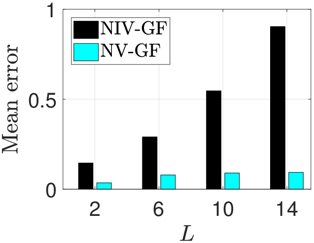
To decide which type of FIR graph filter is more appropriate in WSNs under asymmetric links, we compare for both node-variant and node-invariant GFs, the mean error between performing graph filtering over deterministic graphs and time-varying graphs, where the probabilities of establishing the links are chosen totally randomly and by selecting the optimal coefficients obtained by solving (16) and (17). As it is shown in the example of Fig. 2(a), the node-variant GF has significantly lower mean error among nodes compared to the node-invariant GF. This is due to the fact that node-variant GFs provide higher degree of freedom for choosing the coefficients. For this reason, in this work, node-variant GFs are chosen to conduct distributed graph filtering tasks in random WSNs.

Each entry $p_{ij}$ of the connection probability matrix $\mathbb{P}$ represents, in practice, the Packet Delivery Ratio (PDR) of a given link $(i,j)$ , which is imposed by the WSN environment that is affected by the interference and the background noise. Since the matrix $\mathbb{P}$ may have an impact on the expected error when applying graph filtering, in this work, we analyze a method for adjusting the entries of $\mathbb{P}$ , without considering the case of enforcing equal probabilities for all the links, since this is not realistic in practice. A more realistic approach could be enforcing equal (or similar) entries for each row of the matrix, which reflects in practice equal probabilities of link connections in the neighborhood of a given transmitter node.

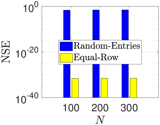
In Fig. 2(b), we analyze the Normalized Squared Error $\text{NSE}=\|\mathbb{H}_{\text{nv}}{-}\sum_{l=0}^{L}{\text{diag}(\boldsymbol{\phi}^{(l)})}{(\mathbb{P}\circ\mathbb{S})}^{l}\|^{2}_{F}/\left\|\mathbb{H}_{\text{nv}}\right\|^{2}_{F}$ between applying graph filtering with node-invariant GF over deterministic graphs and over time-varying graphs, where the optimal coefficients are obtained by solving (17) and the probabilities of establishing the links are adjusted so that $\mathbb{P}$ has equal entries in each row. These adjusted entries correspond to link connection towards neighbors that can be reachable within a given transmission range. The minimum non zero value in each row is used to equalize these entries. As shown in Fig. 2(b), by equalizing the rows of $\mathbb{P}$ , the graph filtering error can be significantly improved. Therefore, we assume in this work that every node $i$ uses a probability $q_{i}$ ( $0<q_{i}\leq 1$ ) to establish a link towards its neighbors, which is equivalent in practice to having each node use a broadcast communication to transmit a packet to its neighbors with this probability, and which should be enforced by an efficient cross-layer distributed MAC protocol. In this paper, the probability $q_{i}$ represents the PDR of a given node $i$ in a WSN. From now on, let us define $\mathbb{Q}$ , which is the connection matrix $\mathbb{P}$ with equalized rows so that $p_{ij}=q_{i}\;\forall j\in\Omega_{i}\;\text{or}\;i=j$ . By establishing the links in the time-varying graph $\mathcal{G}_{t}$ based on the connection probability matrix $\mathbb{Q}$ , the graph shift operator $\bar{\mathbb{S}}$ associated to the expected graph $\bar{\mathcal{G}}$ is given by $\bar{\mathbb{S}}=\mathbb{E}[\mathbb{S}_{t}]=\mathbb{Q}\circ\mathbb{S}$ , that is:

\displaystyle\begin{split}\text{If}\;\mathbb{S}&=\mathbb{A}\;\text{then}\;\bar{\mathbb{S}}=\mathbb{E}[\mathbb{A}_{t}]=\mathbb{Q}\circ\mathbb{A}\\ \text{If}\;\mathbb{S}&=\mathbb{L}\;\text{then}\;\bar{\mathbb{S}}=\mathbb{E}[\mathbb{L}_{t}]=\mathbb{E}[\mathbb{D}_{t}-\mathbb{A}_{t}]=\mathbb{E}[\mathbb{D}_{t}]-\mathbb{E}[\mathbb{A}_{t}]\\ &=\mathbb{Q}\circ\mathbb{D}-\mathbb{Q}\circ\mathbb{A}=\mathbb{Q}\circ(\mathbb{D}-\mathbb{A})=\mathbb{Q}\circ\mathbb{L}\\ \end{split}

This means that by considering the new defined connection probability matrix $\mathbb{Q}$ and in order to minimize the bias, we need to reduce the filtering matrix difference given by:

\mathbb{B}_{\text{eq}}^{\star}=\sum_{l=0}^{L}\left({\text{diag}(\boldsymbol{\phi}^{(l)})}\;{(\mathbb{Q}\circ\mathbb{S})}^{l}-\text{diag}(\boldsymbol{h}^{(l)})\;\mathbb{S}^{l}\right)

(18)

Next, we focus on the variance of the graph filtering, which in addition to the expected error is essential to control the total Mean Squared Error (MSE).

V-B Variance

We focus our analysis on the average variance across the nodes, which can be expressed as:

\overline{var}[\mathbb{y}_{t}]=\big(\text{tr}\big(\mathbb{E}[\mathbb{y}_{t}{\mathbb{y}_{t}}^{H}]-\mathbb{E}[\mathbb{y}_{t}]\mathbb{E}[\mathbb{y_{t}}]^{H}\big)/N

(19)

The main result related to the average variance is given by the following proposition.

Proposition 1.

Consider a node-variant graph filter operating over time-varying networks with links activated based on a connection probability matrix $\mathbb{Q}$ . The average variance across the nodes of the graph filter is upper bounded by:

\displaystyle\begin{split}\overline{var}[\mathbb{y}_{t}]&\leq\frac{{\|\mathbb{x}\|}^{2}}{N}\;\bigg(\displaystyle\sum_{l=0}^{L}\vartheta_{l}\bigg)^{2}\end{split}

(20)

where $\vartheta_{l}=\rho^{l}\;\|{{\text{diag}(\boldsymbol{\phi}^{(l)})}}\|_{2}$ and $\rho$ is an upper bound of the spectral norm of $\mathbb{S}$ .

Proof: See Appendix.

V-C Minimizing the bias-variance trade-off

In order to ensure a total control on the overall MSE, we propose in this section to find the optimal coefficients that minimize a bias-variance trade-off through solving the convex optimization problem:

\begin{array}[]{ll}\underset{\{\boldsymbol{\phi}^{(l)}\}}{\text{minimize}}\left\|\mathbb{B}_{\text{eq}}^{\star}\right\|^{2}_{F}+\mu\;\;\bigg(\displaystyle\sum_{l=0}^{L}\vartheta_{l}\bigg)^{2}\\ \end{array}

(21)

where $\mu$ is a weighting factor trading-off the bias and the upper-bound variance. Note that due to the fact that the positive term ${\|\mathbb{x}\|}^{2}/N$ does not have an influence on the choice of the coefficients and our main focus is to find the coefficients without knowing the input signal, this term is omitted.

Notice that the optimal coefficients that minimize the bias-variance trade-off, when performing distributed graph filtering tasks over random WSNs, depend on the PDRs of the nodes through the connection probability matrix $\mathbb{Q}$ . We will focus in Section VI on how these PDRs can be determined and enforced at the MAC layer by designing a cross-layer protocol.

VI Cross-layer distributed scheduling algorithm for Graph Filtering

In this section, we analyze how to enforce the PDRs at the nodes in a WSN, in order to ensure an accurate graph filtering, through the control of the bias and the variance. As we show in this section, these PDRs can be enforced at the MAC layer by designing a cross-layer distributed scheduling algorithm to be adopted during the communication exchanges among the nodes performing the graph filtering tasks³³ 3 Note that this work can also be easily extended to graph filtering tasks that account for time-varying input signals [35]..

We assume that the time is divided into slots of a fixed duration $\tau$ . At each time slot, a certain number of nodes are allowed to communicate. Our goal is to design a specific scheduling algorithm where the communicating nodes execute the graph filtering steps, resulting into a high accuracy of the filtering process. Without loss of generality⁴⁴ 4 Note that this work does not depend on the specific physical layer of IEEE 802.15.4 and can be easily extended to other physical layers by using other methods to compute the BER., we assume that the WSN uses a similar physical layer as the one corresponding to the standard IEEE 802.15.4 with the 2.4 GHz ISM band⁵⁵ 5 2.4 GHz ISM band has the advantage of being used worldwide without any limitations on applications.. The Bit Error Rate (BER), when node $i$ is transmitting to node $j$ over the link $(i,j)$ , is given by [36]:

\text{BER}_{i,j}=\displaystyle\varsigma_{1}\sum^{\varsigma_{2}}_{k=2}(-1)^{k}e^{\varsigma_{3}\;\text{SINR}_{ij}\;\big(\frac{1}{k}-1\big)}

(22)

where ${\text{SINR}}_{i,j}$ is the received signal to interference plus noise ratio at node $j$ and $\varsigma_{1}$ , $\varsigma_{2}$ and $\varsigma_{3}$ are constants⁶⁶ 6 Note that the constants are based on a realistic analytical model from IEEE 802.15.4 [36]. equal, respectively, to $\frac{1}{30}$ , 16 and 20 as stated in [36].

The PDR of transmitting a packet of length $z$ -bits over a link $(i,j)$ is given by:

\text{PDR}_{i,j}=(1-\text{BER}_{i,j})^{z}

(23)

assuming that the bit errors occur independently across the $z$ -bits of the packet.

Under a physical interference model, the SINR of any link depends on the received signal strength level, which is related to the transmitting power level, the distance between the receiver and the transmitter, and the signal propagation environment. In this paper, in order to estimate the SINR, we adopt the log-distance path-loss propagation model as in [37]. Including fading to this model does not significantly affect the performance in real scenarios, as shown in [38]. According to this model, the received power ${P}_{i,j}$ at a node $j$ from a transmitter node $i$ over a link $(i,j)$ can be expressed as:

{P}_{i,j}=\frac{{P}}{d_{i,j}^{\nu}}

(24)

where $d_{i,j}$ is the distance between both nodes $i$ and $j$ , $\nu$ is the path loss exponent, and ${P}$ is the transmitter power, which is assumed to be the same for all nodes.

The ${\text{SINR}}_{i,j}$ of a link $(i,j)$ is equal to the received power at node $j$ from node $i$ divided by the sum of received powers at node $j$ from all other concurrent transmissions, plus noise.

\text{SINR}_{ij}=\frac{\;{P}_{i,j}}{I_{j}+\mathscr{N}_{0}}

(25)

where $\mathscr{N}_{0}$ is the background noise, which we assume to be constant and known⁷⁷ 7 In practice, this can be estimated through calibration., and $I_{j}$ is the interference experienced at node $j$ , given by $I_{j}=\sum_{u\in\mathcal{V},\;u\neq i}\;{P}_{u,j}$ .

In the SINR-based physical model [29], the successful reception of a packet sent by a node $i$ to a node $j$ is achieved if the SINR at $j$ is higher than a certain value of SINR threshold $\kappa$ , which can be chosen to guarantee a small BER:

\text{SINR}_{ij}=\frac{\;\displaystyle\frac{{P}}{d_{i,j}^{\nu}}}{\sum_{u\in\mathcal{V},\;u\neq i}\;\;\frac{{P}}{d_{u,j}^{\nu}}+\mathscr{N}_{0}}\geq\kappa

(26)

According to the physical interference model, a packet can be correctly received even if there are a single or multiple simultaneous transmitter nodes in the neighborhood of a receiver node $j$ , as far as inequality (26) holds.

Next, we introduce some definitions of specific areas that will be used in the design of our cross-layer distributed scheduling algorithm. The frequently used notations and terminologies are summarized in Table I.

Definition 1.

The maximum transmission radius $R_{\text{m}}$ is defined as the maximum distance up to which a packet sent by a transmitter can be received by every node inside the associated circular area of radius $R_{\text{m}}$ , in absence of interference, which is given by:

R_{\text{m}}=\left(\frac{{P}}{\kappa\;\mathscr{N}_{0}}\right)^{\frac{1}{\nu}}.

(27)

Definition 2.

The broadcast range $R_{\text{B}}$ of every node with transmitter power $P$ , is the distance up to which the node intends to broadcast its messages, when performing graph filtering steps. In general, $R_{\text{B}}$ is lower than $R_{\text{m}}$ due to the presence of interference and can be expressed as:

R_{\text{B}}=\chi\;R_{\text{m}}

(28)

where $0<\chi<1$ and the set of nodes inside the broadcast region of range $R_{\text{B}}$ when a given node $i$ is the transmitter, is denoted as $\Delta^{B}_{i}$ . The neighbors of node $i$ are the nodes within the range $R_{\text{B}}$ .

Given a certain deployment of the nodes, the value of $\chi$ must be selected so that it ensures a connected network, that is, there is a path between every pair of nodes. We will show in Section VI-A how this requirement can be achieved.

Definition 3.

A successful broadcast for a node $i$ is defined as a transmission of a message during the graph filtering process, such that it is successfully received by all receivers $j$ located in the broadcast region within range $R_{\text{B}}$ , where the condition for a successful reception is given by (26).

Figure 3: Collision area and preventing area with an interfering node

u

(

\hat{n}_{I}=1

). Notice that when node

i

is transmitting all nodes inside the blue region are receiving and

j

and

u

can be any point in the perimeters (blue and red).

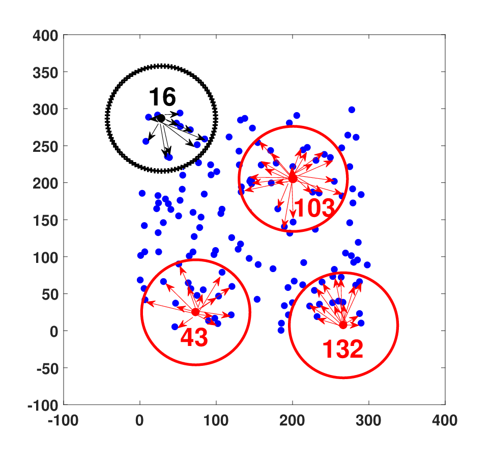
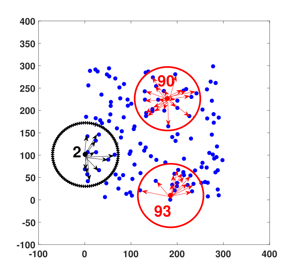
For any transmitter node $i$ in the network, let us consider the worst case of interference experienced by the farthest receiver $j$ located at any point on the perimeter of the broadcast region, i.e., $d_{ij}=R_{\text{B}}$ , and let us assume that there are $\hat{n}_{I}$ interfering nodes whose distances to the receiver are lower bounded by a certain distance $R_{\text{C}}^{\hat{n}_{I}}$ i.e., $d_{uj}\geq R_{\text{C}}^{\hat{n}_{I}},\;\forall\;u\in\mathcal{V},\;u\neq i,\;u\neq j$ , as illustrated in Fig. 3. From (26), we can write that the worst case $\text{SINR}^{(\text{wst})}$ is given by:

\text{SINR}^{\text{wst}}=\frac{\displaystyle\frac{{P}}{R_{\text{B}}^{\nu}}}{\hat{n}_{I}\frac{{P}}{\big(R_{\text{C}}^{\hat{n}_{I}}\big)^{\nu}}+\mathscr{N}_{0}}\geq\kappa\;

(29)

and where, as we explain later in Section VI-A, $\hat{n}_{I}$ is actually an estimation of the number ${n}_{I}$ of interfering nodes, which is computed based on $\hat{N}$ an estimation of the total number of nodes in the network.

Definition 4.

Given a transmitter node with a certain broadcast region of radius $R_{\text{B}}$ , and any receiver node placed at the perimeter of the broadcast region, the collision area is the circular area centered at that receiver, with a radius $R_{\text{C}}^{\hat{n}_{I}}$ given by:

R_{\text{C}}^{\hat{n}_{I}}=\bigg(\frac{\hat{n}_{I}\;\kappa\;{P}\;\;R_{\text{B}}^{\nu}}{{P}-\kappa R_{\text{B}}^{\nu}\;\mathscr{N}_{o}}\bigg)^{\frac{1}{\nu}}.

(30)

Note that $R_{\text{C}}^{\hat{n}_{I}}$ represents the smallest distance (from any intended receiver $j$ ) at which we can have other $\hat{n}_{I}$ transmitters interfering, while still having successful communications at the receivers inside the broadcast region of radius $R_{\text{B}}$ (see Fig. 3). Notice that this radius grows with $\hat{n}_{I}$ , implying that more protection to the receivers is imposed when there are more interfering transmitters.

Definition 5.

The preventing area for a transmitter node is defined as the circular region centered at that node with the radius $R_{P}^{\hat{n}_{I}}$ given by:

R_{P}^{\hat{n}_{I}}=R_{\text{B}}+R_{\text{C}}^{\hat{n}_{I}}

(31)

The preventing area is illustrated in Fig. 3. The set of nodes inside the area of radius $R_{P}^{\hat{n}_{I}}$ for a transmitter node $i$ is denoted by $\Delta^{P}_{i}$ . The ring formed by the outer radius $R_{P}^{\hat{n}_{I}}$ and inner radius $R_{\text{B}}$ contains the locations of the nodes that are responsible for the most significant part of interference experienced by the neighbors of node $i$ , located inside the broadcast area of radius $R_{\text{B}}$ , when receiving from a transmitter node $i$ .

\hat{N}

\text{ID}_{i}

pos_{i}

\tau=0

n_{{t}_{x}}=0

t_{\text{out}}

\text{timer}=0

pkt_{\text{sent}}

pkt_{\text{sent}}

controls the number of packets sent by feasible nodes*/

\tau=\tau+1

;

\mathcal{F}[\tau]=\emptyset

;

pkt_{\text{sent}}=0

state=\text{isActivateNode(}\text{ID}_{i}\text{)}

3: if

state

== ’active’ then

\hat{n}_{I}=\hat{N}-n_{{t}_{x}}-1

\text{send packet with }pos_{i}\text{ and }\hat{n}_{I}

6: reset and trigger timer

7: while

\text{timer}<t_{\text{out}}

8: if receiving packet from feasible nodes then

\text{update }\mathcal{F}[\tau]

10:

\text{check and remove conflicting feasible nodes in }\mathcal{F}[\tau]

11: end if

12: end while

13: if

|\mathcal{F}[\tau]|==\hat{n}_{I}

and

\hat{n}_{I}>0

then

14:

\mathcal{T}_{t_{x}}^{(\tau)}=\mathcal{F}[\tau]\cup\{i\}

; add positions of

\mathcal{T}_{t_{x}}^{(\tau)}

{\xi}^{(\tau)}

15:

n_{{t}_{x}}=n_{{t}_{x}}+|\mathcal{F}[\tau]|+1

16:

\text{send allocated nodes }\mathcal{T}_{t_{x}}^{(\tau)}

{\xi}^{(\tau)}

, and

n_{{t}_{x}}

; exit( )

17: else

18: if

|\mathcal{F}[\tau]|\neq\hat{n}_{I}

and

\hat{n}_{I}>0

then

19:

\hat{n}_{I}=\hat{n}_{I}-1

20: goto line 5

21: else

22:

\mathcal{T}_{t_{x}}^{(\tau)}=\{i\}

;

{\xi}^{(\tau)}=\{pos_{i}\}

23:

n_{{t}_{x}}=n_{{t}_{x}}+1

24:

\text{send allocated nodes }\mathcal{T}_{t_{x}}^{(\tau)}

{\xi}^{(\tau)}

and

n_{{t}_{x}}

; exit( )

25: end if

26: end if

27: else

28: if

\text{receiving }pos_{i}\text{, }\hat{n}_{I}

from active node and

pkt_{\text{sent}}==0

then

29:

\text{compute }R_{\text{C}}^{\hat{n}_{I}}\text{ using (\ref{equation_Rc})}

30:

R_{\text{P}}^{\hat{n}_{I}}=R_{\text{B}}+R_{\text{C}}^{\hat{n}_{I}}

31: reset and trigger timer

32: while

\text{timer}<t_{\text{out}}

33: if overhearing packet from feasible node then

34: store information of overhearing feasible nodes

35: end if

36: end while

37: if Prevent-Condition satisfied and no conflicts then

38:

\text{send packet(}\text{ID}_{i},pos_{i},\textit{'feasible'}\text{) to active node }

39:

pkt_{\text{sent}}=1

40: end if

41: end if

42: if

\text{receiving }\mathcal{T}_{t_{x}}^{(\tau)}

{\xi}^{(\tau)}

and

n_{{t}_{x}}

then

43: if

i\in\mathcal{T}_{t_{x}}^{(\tau)}

then

44: exit( )

45: else

46: goto line 1

47: end if

48: else

49: goto line 28

50: end if

51: end if

Algorithm 1 CDSA algorithm running at each node

i

Table I: Frequently used notations

Parameter	Description	Parameter	Description	Parameter	Description
$L$	Filter order	$\mathbb{S}$	Shift operator	$\mathbb{x}$	Input graph signal
$R_{\text{m}}$	Max. transmission range	$N$	Nr. of nodes	$\mathbb{Q}$	Connection probability matrix
$R_{\text{B}}$	Broadcast range	$P$	Transmission power	$\tau$	Time slot
$\hat{n}_{I}$	Nr. of interfering nodes	$\nu$	Path loss exponent	$T_{s}$	Nr. of allocated slots
$R_{P}^{\hat{n}_{I}}$	Range of preventing area	$\kappa$	SINR threshold	$\mathcal{T}_{t_{x}}^{(\tau)}$	Set of transmitters at slot $\tau$
$R_{C}^{\hat{n}_{I}}$	Range of collision area	$\mathscr{N}_{0}$	Background noise	$n_{{t}_{x}}$	Nr. of current allocated slots

VI-A Cross-layer Distributed Scheduling Algorithm (CDSA)

Given a set of $N$ transmitter nodes that intend to broadcast a packet inside an area of radius $R_{\text{B}}$ , in order to perform the graph filtering steps by means of communication exchanges, our goal is to design a scheduling protocol that activates simultaneously, at each time slot $\tau$ , a disjoint subset of transmitters $\mathcal{T}_{t_{x}}^{(\tau)}\subset\mathcal{V}$ such that $\cup^{\tau=T_{s}}_{\tau=1}\mathcal{T}_{t_{x}}^{(\tau)}=\mathcal{V}$ , and by ensuring at each slot $\tau$ that the SINR of all receivers inside each broadcast region of each activated transmitter is higher that $\kappa$ , and where the $T_{s}$ is the total number of slots. Therefore, the aim is to schedule all these requests in a small number of slots $T_{s}$ and satisfying:

\text{SINR}^{(\tau)}_{j}=\frac{\frac{{P}}{d_{i,j}^{\nu}}}{\displaystyle\sum_{u\in\mathcal{T}_{t_{x}}^{(\tau)}\setminus\{i\}}\frac{{P}}{{d}^{\nu}_{u,j}}+\mathscr{N}_{0}}\geq\kappa,\forall j\in\Delta^{B}_{i},\forall i\in\mathcal{T}_{t_{x}}^{(\tau)},\forall\tau

(32)

so that all the graph filtering steps are carried out as quickly as possible, maximizing time efficiency.

On the one hand, we are interested in ensuring successful simultaneous broadcasting of the transmitters scheduled at each of the time slots and on the other hand, in order to ensure accurate filtering, our protocol should also control, at each transmitter, the PDRs of its corresponding neighbor nodes.

We assume that each node $i$ has an unique identifier ${\text{ID}_{i}}$ and knows its position $pos_{i}$ by using a geo-localization system or acquiring its location during the initial network setup, for instance as described in [39]. Every node can also estimate its distance to its neighbors inside the broadcast area by means of exchanging information locations or using signal detection techniques, such as in [40]. Moreover, every node can determine an estimate $\hat{N}$ of the total number of nodes in the network by using one of the well known distributed algorithm for counting the number nodes in WSNs, based on consensus (e.g., [41]). As explained next, the accuracy of the estimated total number of nodes does not have a significant impact on the allocation of slots obtained by our proposed scheduling algorithm since this value is only used as a starting point in the execution of the algorithm.

In our proposed cross-layer scheduling algorithm, which we call CDSA, during the allocation of a certain time slot $\tau$ , the nodes are classified into one of these three sets, each one corresponding to a certain state:

•

Active node ( $\mathcal{A}[\tau]$ ): When a single node is activated to initiate the allocation of transmitter nodes for the slot $\tau$ , it belongs to this state.
•

Feasible nodes ( $\mathcal{F}[\tau]$ ): When a node has its preventing area of radius $R_{P}^{\hat{n}_{I}}$ outside the preventing area of the active node, it belongs to this state. This implies that this node can potentially be selected as a transmitter in the slot $\tau$ .
•

Candidate nodes ( $\mathcal{C}[\tau]$ ): Every node that is neither in Active or Feasible state and that has not yet been allocated a slot, belongs to this state.

Initially, the states of the nodes are as follows: $\mathcal{A}[0]=\emptyset$ , $\mathcal{F}[0]=\emptyset$ , $\mathcal{C}[0]=\mathcal{V}$ . Let $n_{{t}_{x}}$ denote the current total number of nodes that have been allocated transmission slots (initially $n_{{t}_{x}}=0$ ) and ${\xi}^{(\tau)}$ the set of positions of the nodes allocated at slot $\tau$ . As shown in Algorithm 1, a single node $i$ , randomly selected from the candidate set $\mathcal{C}[\tau]$ , is initially activated to initiate the allocation of transmitters at slot $\tau$ , allowing thus to select the nodes that can transmit simultaneously with it at the same slot $\tau$ . First, the active node $i$ sends to all other nodes its position $pos_{i}$ and the current estimated number of interfering nodes $\hat{n}_{I}$ , which is computed from the estimation of the total number of nodes as $\hat{n}_{I}=\hat{N}-n_{{t}_{x}}-1$ . Then, the states of nodes become as follows: $\mathcal{A}[\tau]=\{i\}$ , $\mathcal{C}[\tau]=\mathcal{V}\setminus\{\{i\}\cup\mathcal{T}^{(\tau-1)}_{a}\cup\ldots\cup\mathcal{T}^{(0)}_{a}\}$ , $\tau=1$ .

At a certain slot $\tau$ , every node $u\in\mathcal{C}[\tau]$ computes the radius of the collision area $R_{\text{C}}^{\hat{n}_{I}}$ by using (30) and the received value $\hat{n}_{I}$ . Then, it computes its preventing range $R_{P}^{\hat{n}_{I}}$ by using (31). In order to be able to satisfy (32), the node $u$ must have its preventing area of radius $R_{P}^{\hat{n}_{I}}$ outside the preventing areas of the active node $i$ and of the other feasible nodes⁸⁸ 8 Notice that, a candidate node can overhear some feasible nodes in its neighborhood but it cannot have the knowledge of all the feasible nodes. in $\mathcal{F}[\tau]$ , as shown in Fig. 4. We refer to the condition where the preventing area of a candidate node $u$ is outside the preventing area of the active node as Prevent-Condition. Any node $u$ checks if it satisfies the Prevent-Condition and if its preventing area is not overlapping with any potentially overhearing feasible nodes in its neighborhood. This overlapping occurs when the distance between two nodes is less than twice of the preventing radius. If both conditions are satisfied, the node $u$ sends a packet with its position $pos_{u}$ and its state as potential feasible node to the active node $i$ . As a result, the active node $i$ makes the update $\mathcal{F}[\tau]=\mathcal{F}[\tau]\cup\{u\}$ . Note that the knowledge of the state of the nodes (i.e., $\mathcal{A}[\tau]$ , $\mathcal{F}[\tau]$ and $\mathcal{C}[\tau]$ ) does not need to be known and shared among all the nodes. Only the active node at a given time slot $\tau$ needs to keep the set of feasible nodes that have notified to it.

After a predefined timeout⁹⁹ 9 This maximum timeout can be estimated by taking into account the number of nodes and the delays related to transmission, reception and propagation. $t_{\text{out}}$ that ensures the reception of the packets from all potential feasible nodes, the active node $i$ checks if there are some nodes in $\mathcal{F}[\tau]$ that have their corresponding preventing areas overlapping. This problem may happen when two or more nodes change their states at the same time instant, without hearing each other or when they are outside the transmission ranges of each other. The active node resolves the conflict¹⁰¹⁰ 10 A simple way to resolve this conflict is to consider the order of receiving the feasible nodes by keeping adding as feasible node only the node that does not conflict with the previous selected feasible nodes. We leave the extention to more advanced approaches to solve this conflict for future research. by keeping only one of the conflicting feasible nodes. Next, in order to be able to decide which nodes will be selected as transmitters at slot $\tau$ , the active node $i$ compares the number of feasible nodes and the number of interfering nodes:

$\bullet$ If $|\mathcal{F}[\tau]|\neq\hat{n}_{I}$ , the active node $i$ decreases the estimated number of interfering nodes $\hat{n}_{I}=\hat{n}_{I}-1$ if $\hat{n}_{I}>0$ and sends this new value to all other nodes that have not yet been allocated a slot. The process is repeated by making the active node $i$ and the candidate nodes in $\mathcal{C}[\tau]$ update their preventing range $R_{P}^{\hat{n}_{I}}$ based on the new value of $\hat{n}_{I}$ and checking again if the Prevent-Condition is satisfied. Note that after this, the set $\mathcal{F}[\tau]$ will also change. Notice also that in order to reduce the overhead of these control packets, every candidate node only needs to send once a control packet informing about the potential feasibility to the same current active node, which has to check for any new updated preventing area if previous received feasible nodes are still not conflicting with each other and satisfy the Prevent-Condition.

$\bullet$ If $|\mathcal{F}[\tau]|=\hat{n}_{I}$ , the active node $i$ sends a packet to inform the candidate and feasible nodes that the nodes in $\mathcal{F}[\tau]$ have been allocated the slot $\tau$ $\big($ i.e., $\mathcal{T}_{t_{x}}^{(\tau)}=\mathcal{F}[\tau]\cup\{i\}\big)$ , their positions are ${\xi}^{(\tau)}$ and the total number of allocated nodes is now $n_{{t}_{x}}$ , where $n_{{t}_{x}}=n_{{t}_{x}}+|\mathcal{F}[\tau]|+1$ . Then, the process continues to determine the nodes that will be allocated in the following slot $\tau+1$ , by activating randomly a new node $i^{\prime}$ from the remaining candidate transmitter set $\mathcal{C}[\tau+1]$ , where $\mathcal{C}[\tau+1]=\mathcal{C}[\tau]\setminus\mathcal{T}_{t_{x}}^{(\tau)}$ , $\mathcal{F}[\tau+1]=\emptyset$ , $\mathcal{A}[\tau+1]=\{i^{\prime}\}$ . The new active node $i^{\prime}$ sets the number of interfering nodes to $\hat{n}_{I}=\hat{N}-n_{{t}_{x}}-1$ and informs other nodes. Then, the process is repeated by making every candidate node determine its new preventing range $R_{P}^{\hat{n}_{I}}$ based on the new value of $\hat{n}_{I}$ and checking if it satisfies the Prevent-Condition and does not conflict with potentially overhearing feasible nodes.

$\bullet$ If the estimated number of interfering nodes reaches zero ( $\hat{n}_{I}=0$ ), only the active node $i$ is assigned the current slot $\tau$ $\big($ i.e., $\mathcal{T}_{t_{x}}^{(\tau)}=\{i\}\big)$ with $n_{{t}_{x}}=n_{{t}_{x}}+1$ . Then, for the next slot $\tau+1$ , we have $\mathcal{C}[\tau+1]=\mathcal{C}[\tau]\setminus\{i\}$ , $\mathcal{F}[\tau+1]=\emptyset$ . The process is repeated so that a new candidate node from $\mathcal{C}[\tau+1]$ is randomly chosen as active node. This implies setting $\hat{n}_{I}=\hat{N}-n_{{t}_{x}}-1$ and checking which candidate nodes satisfy the Prevent-Condition and do not conflict with potentially overhearing feasible nodes.

The algorithm stops whenever there is no node that needs to determine its allocation slot, which means that the candidate set becomes empty $\mathcal{C}[\tau]=\emptyset$ . At the end of the algorithm, every transmitter $i$ knows its assigned slot $\tau$ , the number of other nodes that will transmit at the same time slot $\tau$ and their positions ${\xi}^{(\tau)}$ . Thus, every transmitter $i$ is able to compute the smallest SINR in its neighborhood, given by:

{\text{SINR}}^{\text{min}}_{i}=\min_{j\in\Delta^{B}_{i}}\left(\frac{\;\displaystyle\frac{{P}}{d_{i,j}^{\nu}}}{\displaystyle\sum_{u\in\mathcal{T}_{t_{x}}^{(\tau)},\;u\neq i}\;\;\frac{{P}}{d_{u,j}^{\nu}}+\mathscr{N}_{0}}\right),\;i\in\mathcal{T}_{t_{x}}^{(\tau)}

(33)

Then, the main idea is that each transmitter $i$ can adjust the PDRs of its neighbors within its broadcast area to make them equal, which is necessary to maximize the accuracy of the graph filtering process, as shown in Section V, by setting them to $\text{PDR}^{\text{min}}_{i}$ , which refers to the minimum PDR of node $i$ when broadcasting to its neighbors within the range $R_{\text{B}}$ . Notice that $\text{PDR}^{\text{min}}_{i}$ can be readily obtained from the $\text{SINR}^{\text{min}}_{i}$ estimated in the neighborhood of node $i$ , by using (22) and (23), as follows:

\text{PDR}^{\text{min}}_{i}=\bigg(1-\varsigma_{1}\displaystyle\sum^{\varsigma_{2}}_{k=2}(-1)^{k}e^{\varsigma_{3}\;\text{SINR}^{\text{min}}_{i}\;\big(\frac{1}{k}-1\big)}\bigg)^{z}

(34)

In order to equalize the PDRs, each transmitter $i$ broadcasts a packet to all its neighbors $j\in\Delta^{B}_{i}$ , but imposes for each neighbor $j$ a different probability of acceptance $p^{(\text{ac})}_{ij}$ to accept the reception of the packet, and which is chosen such that:

\text{PDR}^{\text{min}}_{i}=p^{(\text{ac})}_{ij}\;\text{PDR}_{ij},\;i\in\mathcal{V},\;{\forall j\in\Delta^{B}_{i}}.

(35)

In other words, for a given probability $p^{(\text{ac})}_{ij}$ , the transmitter $i$ , during its allocated slot $\tau$ , specifies in every packet it broadcasts, the identifier of the nodes that have to accept the received packet with proportions that match $p^{(\text{ac})}_{ij}$ . Other nodes simply ignore the packet. It is important to notice that this is due to the fact that our protocol is designed for ensuring accuracy in the filtering operations, as opposed to the case of maximizing throughput of bits.

The use of the probability $p^{(\text{ac})}_{ij}$ leads to the adjusted values of PDRs that allow to determine the desired connection probability matrix $\mathbb{Q}$ , as shown in Section V. Then, the filter coefficients can be easily optimized by using (21). As our experimental results show in Section VII, each node can perform the distributed graph filtering task with high accuracy due to the control of the resulting bias and variance of the graph filtering process.

As mentioned earlier, in order to maximize the time efficiency in our graph filtering, our scheduling protocol aims at minimizing the total number of slots. The main result is given by the following proposition.

Proposition 2.

Consider $N$ sensor nodes deployed uniformly random inside a 2-D square area of side length $\ell_{s}$ . In order to decrease the number of allocated slots in our CDSA protocol, thus allowing a higher number of simultaneous transmissions, the probability of having all nodes inside a disc of radius $R^{\ast}_{P}$ has to be reduced by increasing the probability that there are any two nodes located at a distance higher than $2\;R^{\ast}_{P}$ . This can be achieved if $\ell_{s}$ is selected such as $\ell_{s}>>R^{\ast}_{P}$ and reducing the value of $\chi$ while still maintaining the connectivity of the whole network ( $\ell_{s}\sqrt{(\pi NR^{2}_{\text{m}})^{-1}\log{N}}<\chi<1$ ), where $R^{\ast}_{P}$ is given by:

R^{\ast}_{P}=R_{P}^{\hat{n}_{I}=1}=\chi\;\bigg(\frac{{P}}{\kappa\;\mathscr{N}_{0}}\bigg)^{\frac{1}{\nu}}+\bigg(\frac{\;\kappa\;{P}\;\;R_{\text{B}}^{\nu}}{{P}-\kappa R_{\text{B}}^{\nu}\;\mathscr{N}_{o}}\bigg)^{\frac{1}{\nu}}

Proof: See Appendix.

Remark 2.

The proposed CDSA algorithm is designed for sensor nodes that perform many iterations of graph filtering process. In order to reduce the control communication, these nodes can keep their allocated slots in several iterations of the different graph filtering operations even though there are some link losses. This is because the graph filters are designed to be robust to network topology changes, through the optimization of the filter coefficients.

VII Numerical experiments

This section validates our theoretical findings, where several experiments are conducted in Matlab to evaluate the performance of our proposed solutions. WSNs with $N$ sensor nodes are randomly and uniformly distributed over a square area of side $\ell_{s}$ m. Each node can communicate with the neighbors within its broadcast range given by $R_{B}=\chi\left(P/(\kappa\;\mathscr{N}_{0})\right)^{\frac{1}{\nu}}$ . We consider the input graph signal, acquired by the WSN, given by $\mathbb{x}=\mathbb{v}+\mathbb{n}$ , where $\mathbb{v}$ is the smooth true graph signal and $\mathbb{n}$ is a zero mean Gaussian noise with $0.1$ standard deviation. In order to impose a small spectral norm that can further decrease the variance, the shift operator used is $\mathbb{S}=\lambda_{\max}^{-1}\mathbb{L}-0.5\mathbb{I}$ , where $\lambda_{\max}$ is the maximum eigenvalue of $\mathbb{L}$ . We analyze the error $\mathbb{e}=\mathbb{y}_{t}{-}\mathbb{y}$ and the empirical variance of the error averaged over all nodes and realizations, that is, ${{\overline{\sigma}}_{\mathbb{e}}^{2}}=\text{tr}(\mathbb{E}[\mathbb{e}\mathbb{e}^{H}])/N$ , which can approach the average variance $\overline{var}[\mathbb{y}_{t}]$ for a sufficiently high number of realizations. The filter coefficients used when operating filtering over time-varying networks are optimized as presented in Section V-C. The results are obtained by averaging over 1000 realizations of graphs.

Fig. 5 plots the mean error averaged over all the nodes and realizations, as well as the empirical average variance ${{\overline{\sigma}}_{\mathbb{e}}^{2}}$ , for different probabilities $q_{i}$ of link activation. As expected, it can be seen in Fig. 5(a)-(b) that node-variant GF has significantly better performance than the node-invariant GF, where in both filters the coefficients are optimized. This is due to the higher number of degrees of freedom that node-variant GF can offer to choose the coefficients, as compared to the node-invariant GF, where the same coefficients are used by all nodes. In Fig. 5(c)-(d), we can observe that by using node-variant GFs with optimized filter coefficients, a small mean error in the order of $10^{-2}$ and a low empirical average variance in the order of $10^{-3}$ are obtained for $q_{i}\geq 0.55$ . This also means that the output of graph filtering over the deterministic graph $\mathcal{G}_{0}$ is very close to the one obtained on average over the time-varying graph $\mathcal{G}_{t}$ , indicating that a high filtering accuracy is achieved. As expected, it can also be noticed that better link connectivities (i.e., higher $q_{i}$ ’s) lead to higher graph filtering accuracy.

We evaluate also the performance of applying graph filtering in random WSNs, by comparing at MAC layer, our proposed CDSA protocol with the three state-of-the-art algorithms that allow asymmetric links, namely LBPIM [22], RLBA [13] and SDDC [28]. Fig. 6(a) shows that our proposed protocol CDSA significantly outperforms the existing algorithms in term of the resulting Normalized Squared Error $\text{NSE}=\|\mathbb{y}-\bar{\mathbb{y}}_{t}\|^{2}/\|\mathbb{y}\|^{2}$ of the graph filtering. In fact, compared to the existing algorithms, our CDSA protocol controls the PDRs, which ensures the accuracy of the filtering operations. Fig. 6(b) shows that increasing the transmission power, increases the NSE, which is caused by the fact that more errors are generated due to involving more nodes inside a larger broadcast area, where the graph filtering tasks are performed. Nevertheless, our CDSA protocol still achieves the highest filtering accuracy, which can be even reached in a single filtering iteration. Fig. 6(c) shows the impact of the threshold $\kappa$ on the NSE of graph filtering. Indeed, increasing the threshold $\kappa$ improves the SINR at the receivers as well as the PDRs, which reduces the resulting filtering error.

Fig. 7 illustrates the number of time slots $T_{s}$ until all nodes perform a successful local broadcast per graph filtering iteration, which accounts for the total delay per graph filtering operation. The results show that our CSDA algorithm achieves lower delay compared to the three other protocols. This can be explained by the fact that our CSDA protocol controls the PDRs and takes into account the number of interfering nodes and their locations to determine the preventing area when allocating the slots, ensuring that the SINR at all receivers is always higher than $\kappa$ . This approach is different from the ones used by the three other protocols, where each node can transmit with a certain probability in each slot, without considering the number of interfering nodes.

Fig. 8 shows two examples of denoising by graph filtering in two different topologies, namely, a $10{\times}10$ -grid and random WSNs, where different scheduling algorithms are used. The average graph signal output obtained by graph filtering in time-varying WSNs when using CDSA protocol, is the one that matches better the graph signal output obtained by graph filtering in the deterministic WSN with perfect MAC environment (i.e., absence of interference and background noise). This is due to the fact that our CDSA protocol imposes during the slot allocation a preventing area that takes into account the number of interfering nodes and controls the PDRs at each broadcast region to improve the graph filtering accuracy.

VIII Conclusion

In this work, we first study and characterize the graph filtering error and show that for both types of FIR GFs (node-invariant and node-variant), equal probabilities for all the links, enables to have an unbiased filtering, which cannot be achieved in practice in WSNs due to interferences and noise. Then, we present an efficient and robust design strategy to perform graph filtering tasks over random WSNs with node-variant graph filters by maximizing accuracy that is, optimizing a bias-variance tradeoff. The accuracy and the efficiency of the graph filtering process, which is implemented distributedly by means of cooperation and communication exchanges between the sensor nodes, is enforced at the MAC layer by designing a Cross-layer Distributed Scheduling Algorithm. As illustrated in the experiments, a high filtering accuracy is obtained when our proposed CDSA protocol combined with optimized graph filtering coefficients is used, allowing to obtain higher performance for the denoising application, as compared to the best existing state-of-art algorithms.

Conditions for obtaining an unbiased graph filtering

In order to obtain an unbiased filtering i.e., $\bar{\mathbb{e}}=\mathbb{0}$ , we must have:

\displaystyle\sum_{l=0}^{L}\phi_{l}\;\bar{\mathbb{S}}^{l}\;\mathbb{x}=\displaystyle\sum_{l=0}^{L}h_{l}\;\mathbb{S}^{l}\;\mathbb{x}

(36)

which is equivalent to enforce the following:

\phi_{0}=h_{0}\;\;\;\text{and}\;\;\displaystyle\sum_{l=1}^{L}{\big({\phi_{l}}^{\frac{1}{l}}\;\bar{\mathbb{S}}\big)}^{l}\;\mathbb{x}=\displaystyle\sum_{l=1}^{L}\big({h_{l}^{\frac{1}{l}}\;\mathbb{S}}\big)^{l}\;\mathbb{x}

(37)

If we select $\phi_{0}=h_{0}$ and ${\phi_{l}}^{\frac{1}{l}}\;\bar{\mathbb{S}}={h_{l}^{\frac{1}{l}}\;\mathbb{S}}$ for $l\geq 1$ , we have $\bar{\mathbb{e}}=\mathbb{0}$ , implying that we can write the following conditions:

\displaystyle{\phi_{l}}^{\frac{1}{l}}\bar{\mathbb{S}}

\displaystyle=\begin{bmatrix}{\phi_{l}}^{\frac{1}{l}}p_{11}s_{11}&{\phi_{l}}^{\frac{1}{l}}p_{12}s_{12}&\cdots&{\phi_{l}}^{\frac{1}{l}}p_{1N}s_{1N}\hskip-5.69046pt\\ {\phi_{l}}^{\frac{1}{l}}p_{21}s_{21}&{\phi_{l}}^{\frac{1}{l}}p_{22}s_{22}&\cdots&{\phi_{l}}^{\frac{1}{l}}p_{2N}s_{2N}\hskip-5.69046pt\\ \vdots&\vdots&\vdots&\vdots&\hskip-5.69046pt\\ {\phi_{l}}^{\frac{1}{l}}p_{N1}s_{N1}&{\phi_{l}}^{\frac{1}{l}}p_{N2}s_{N2}&\cdots&{\phi_{l}}^{\frac{1}{l}}p_{NN}s_{NN}\hskip-5.69046pt\end{bmatrix}

(38)

\displaystyle={h_{l}^{\frac{1}{l}}\mathbb{S}}=\begin{bmatrix}{h_{l}}^{\frac{1}{l}}s_{11}&{h_{l}}^{\frac{1}{l}}s_{12}&\cdots&{h_{l}}^{\frac{1}{l}}s_{1N}\\ {h_{l}}^{\frac{1}{l}}s_{21}&{h_{l}}^{\frac{1}{l}}s_{22}&\cdots&{h_{l}}^{\frac{1}{l}}s_{2N}\\ \vdots&\vdots&\vdots&\vdots&\\ {h_{l}}^{\frac{1}{l}}s_{N1}&{h_{l}}^{\frac{1}{l}}s_{N2}&\cdots&{h_{l}}^{\frac{1}{l}}s_{NN}\end{bmatrix}

which means that we need to impose the following conditions:

	$\displaystyle{\phi_{l}}^{\frac{1}{l}}p_{ii}s_{ii}$	$\displaystyle={h_{l}}^{\frac{1}{l}}s_{ii}$
	$\displaystyle{\phi_{l}}^{\frac{1}{l}}p_{ij}s_{ij}$	$\displaystyle={h_{l}}^{\frac{1}{l}}s_{ij},\;\;\;\;\;\;\forall i,j,\;\;l\geq 1$
	$\displaystyle{\phi_{l}}^{\frac{1}{l}}p_{ji}s_{ji}$	$\displaystyle={h_{l}}^{\frac{1}{l}}s_{ji}$

Therefore, it can be easily seen that to obtain $\bar{\mathbb{e}}=\mathbb{0}$ , the links need to be activated with an equal probability $p$ and the coefficients have to meet the following requirements:

\phi_{l}=p_{ij}^{-l}\;\;{h_{l}}=p_{ji}^{-l}\;\;{h_{l}}=p_{ii}^{-l}\;\;{h_{l}}={p}^{-l}\;h_{l}\;\;\forall i,j,l

(39)

Proof of Proposition 1

By considering the linearity of expectation and trace, the first term on the right side of (19) can be written as [9]:

\begin{split}\text{tr}(\mathbb{E}\big[\mathbb{y}_{t}{\mathbb{y}_{t}}^{H}])&={\!\sum^{L}_{k=0,l=0}}\Lambda(k,l)\end{split}\vskip-7.11317pt

(40)

where:

\begin{split}\Lambda(k,l)=&\text{tr}\bigg(\mathbb{E}\bigg[\text{diag}(\boldsymbol{\phi}^{(k)})\mathbb{\Theta}(t,t-k+1)\;\mathbb{x}\mathbb{x}^{H}\\ &\times{\mathbb{\Theta}(t,t-l+1)}^{H}{{\text{diag}(\boldsymbol{\phi}^{(l)})}^{H}}\bigg]\bigg).\end{split}\vskip-7.11317pt

(41)

By considering the fact that the trace is commutative with respect to the expectation and invariant under cyclic permutations i.e., $\text{tr}(\mathbb{M}\mathbb{W}\mathbb{Z})=\text{tr}(\mathbb{Z}\mathbb{M}\mathbb{W})$ , we can write:

\begin{split}&\Lambda(k,l)=\mathbb{E}\bigg[tr\big(\;\text{diag}(\boldsymbol{\phi}^{(k)})\;\mathbb{\Theta}(t,t-k+1)\;\mathbb{x}\mathbb{x}^{H}{\mathbb{\Theta}(t,t-l+1)}^{H}\\ &\times{diag(\boldsymbol{\phi}^{(l)})}^{H}\big)\bigg]\\ &{=}\text{tr}\big(\mathbb{E}\big[{\mathbb{\Theta}(t,t-l+1)}^{H}{\text{diag}(\boldsymbol{\phi}^{(l)})}^{H}\text{diag}(\boldsymbol{\phi}^{(k)})\;\mathbb{\Theta}(t,t-k+1)\big]\mathbb{x}\mathbb{x}^{H}\big)\\ \end{split}\vskip-7.11317pt

(42)

By making the observation that for any square matrix $\mathbb{M}$ and a positive semi-definite matrix $\mathbb{W}$ , the inequality $\text{tr}(\mathbb{M}\mathbb{W})\leq\|\mathbb{M}\|_{2}\;\text{tr}(\mathbb{W})$ [42] holds, and then applying it to (42), we can write:

\begin{split}&\Lambda(k,l){\leq}\big\|\mathbb{E}\big[{\mathbb{\Theta}(t,t-l+1)}^{H}{{\text{diag}(\boldsymbol{\phi}^{(l)})}^{H}}\text{diag}(\boldsymbol{\phi}^{(k)})\\ &\times\mathbb{\Theta}(t,t-k+1)\big]\big\|_{2}\;tr\big(\mathbb{x}\mathbb{x}^{H}\big)\end{split}

(43)

By applying the Jensen’s inequality of the spectral norm $\|\mathbb{E}[\mathbb{M}]\|_{2}\leq\mathbb{E}[\|\mathbb{M}\|_{2}]$ and the sub-multiplicativity property of the spectral norm of a square matrix $\|\mathbb{M}\mathbb{W}\|_{2}\leq\|\mathbb{M}\|_{2}\|\mathbb{W}\|_{2}$ , we obtain:

\begin{split}&\Lambda(k,l){\leq}\mathbb{E}\big[\big\|\;{\mathbb{\Theta}(t,t-l+1)}^{H}{\text{diag}(\boldsymbol{\phi}^{(l)})}^{H}\text{diag}(\boldsymbol{\phi}^{(k)})\;\mathbb{\Theta}(t,t-k+1)\big\|_{2}\big]\\ &\times tr\big(\mathbb{x}\;\mathbb{x}^{H}\big)\\ &{\leq}\mathbb{E}\bigg[\big\|\big(\prod_{\tau=t}^{t-l+1}\!\!\mathbb{S}_{\tau}\big)^{H}\big\|_{2}{\|{{\text{diag}(\boldsymbol{\phi}^{(l)})}^{H}}\|}_{2}{\|\text{diag}(\boldsymbol{\phi}^{(k)})\|}_{2}\;\big\|\big(\prod_{\tau=t}^{t-k+1}\!\!\mathbb{S}_{\tau}\big)\big\|_{2}\bigg]{\|\mathbb{x}\|}^{2}\\ &{\leq}\rho^{l+k}\;\|{{\text{diag}(\boldsymbol{\phi}^{(l)})}}\|_{2}\;\|\text{diag}(\boldsymbol{\phi}^{(k)})\|_{2}\;\;{\|\mathbb{x}\|}^{2}\end{split}

(44)

where we assume here an upper-bounded spectral norm of the shift operator i.e., $\|\mathbb{S}_{t}\|_{2}\leq\|\mathbb{S}\|_{2}\leq\rho$ for all $t$ [20, 43], implying that:

\displaystyle\begin{split}\text{tr}(\mathbb{E}\big[\mathbb{y}_{t}{\mathbb{y}_{t}}^{H}])&\leq\displaystyle\sum_{{k=0},{l=0}}^{L}\rho^{l+k}\;\|{{\text{diag}(\boldsymbol{\phi}^{(l)})}}\|_{2}\;\|\text{diag}(\boldsymbol{\phi}^{(k)})\|_{2}\;\;{\|\mathbb{x}\|}^{2}\\ &\leq\;{\|\mathbb{x}\|}^{2}\big(\rho^{0}\|{{\text{diag}(\boldsymbol{\phi}^{(0)})}}\|_{2}+\rho^{1}\|{{\text{diag}(\boldsymbol{\phi}^{(1)})}}\|_{2}+..\\ &+\rho^{L}\|{{\text{diag}(\boldsymbol{\phi}^{(L)})}}\|_{2}\big)^{2}\\ \end{split}

(45)

Observe that the second term in (19) is positive i.e., $\text{tr}(\mathbb{E}[\mathbb{y}_{t}]\mathbb{E}[\mathbb{y_{t}}]^{H}){\geq}0$ . Then, if we divide both sides by $N$ in (45) and operate, $\overline{var}[\mathbb{y}_{t}]$ can be upper bounded by (20).∎

Proof of Proposition 2

The disc of radius $R^{\ast}_{P}=R_{P}^{\hat{n}_{I}=1}$ corresponds to the preventing area used by our CDSA protocol when assigning slots in the case that there are at most two nodes that can transmit simultaneously, which corresponds to one transmitter and one interfering node i.e., $\hat{n}_{I}=1$ . If all the $N$ sensor nodes are located inside a disc of radius $R^{\ast}_{P}$ , this means that $\forall i\in\mathcal{V}\;\text{and}\;\forall j\in\mathcal{V}$ , the distance $d_{i,j}\leq 2\;R^{\ast}_{P}$ , which means that in the whole network, there is no node $i$ that can simultaneously transmit with another node $j$ , because our CDSA protocol cannot allocate the same slot to these nodes to transmit simultaneously. This is due to the fact that their preventing areas are overlapping. Therefore, each node will be allocated a slot to transmit exclusively alone, making the total number of allocated slots $T_{s}$ equal to $N$ . This implies that the number of slots is $T_{s}=N$ if and only if there exists a disc of radius $R^{\ast}_{P}$ that contains all the $N$ nodes. In addition to that, by considering that the $N$ sensor nodes are deployed uniformly random inside a 2-D square area of side length $\ell_{s}$ , the probability that there are any two nodes located at a distance shorter than $2\;R^{\ast}_{P}$ , is simply given by:

\text{prob}_{1}=\frac{\pi(2{R^{\ast}_{P}})^{2}}{{\ell_{s}}^{2}}

(46)

This means that the probability that there are any two nodes located at a distance larger than $2\;R^{\ast}_{P}$ , is given by:

\text{prob}_{2}=1-\text{prob}_{1}=1-\frac{\pi(2{R^{\ast}_{P}})^{2}}{{\ell_{s}}^{2}}

(47)

Therefore, to decrease the number of allocated slots in our CDSA protocol, the probability of having all nodes inside a disc of radius $R^{\ast}_{P}$ should be decreased, by increasing the probability that there are any two nodes located at a distance higher than $2\;R^{\ast}_{P}$ . This can be achieved if the side of the deployed square area $\ell_{s}$ is selected such that $\ell_{s}>>R^{\ast}_{P}$ and by reducing the value of $\chi$ while still maintainting the connectivity of the whole network. Thus, a small value of $\chi$ can be selected in the range $\ell_{s}\sqrt{(\pi NR^{2}_{\text{m}})^{-1}\log{N}}<\chi<1$ , since for large-scale networks deployed randomly and uniformly, the critical radius for connectivity is $\ell_{s}\sqrt{(\pi N)^{-1}\log{N}}$ , as shown in [29, 44].∎

References

[1] L. B. Saad and B. Beferull-Lozano, “Stochastic graph filtering under asymmetric links in wireless sensor networks,” in Proc. IEEE Int. Workshop Sig. Process. Advances Wireless Commun., Jun 2018, pp. 1–5.
[2] D. I. Shuman, S. K. Narang, P. Frossard, A. Ortega, and P. Vandergheynst, “The emerging field of signal processing on graphs: Extending high-dimensional data analysis to networks and other irregular domains,” IEEE Sig. Process. Mag., vol. 30, no. 3, pp. 83–98, May 2013.
[3] A. Sandryhaila and J. M. F. Moura, “Discrete signal processing on graphs: Frequency analysis,” IEEE Trans. Sig. Process., vol. 62, no. 12, pp. 3042–3054, Jun 2014.
[4] D. I. Shuman, P. Vandergheynst, and P. Frossard, “Chebyshev polynomial approximation for distributed signal processing,” in Proc. Int. Conf. on Distributed Comput. in Sensor Syst. and Workshops, Jun 2011, pp. 1–8.
[5] A. Sandryhaila and J. M. F. Moura, “Big data analysis with signal processing on graphs: Representation and processing of massive data sets with irregular structure,” IEEE Sig. Process. Mag., vol. 31, no. 5, pp. 80–90, Sep 2014.
[6] A. Sandryhaila, S. Kar, and J. M. F. Moura, “Finite-time distributed consensus through graph filters,” in Proc. IEEE Int. Conf. Acoust., Speech, Sig. Process., May 2014, pp. 1080–1084.
[7] S. Chen, A. Sandryhaila, J. M. F. Moura, and J. Kovacevic, “Signal denoising on graphs via graph filtering,” in Proc. Global Conf. Sig. Inf. Process., Dec 2014, pp. 872–876.
[8] J. Ma, W. Huang, S. Segarra, and A. Ribeiro, “Diffusion filtering of graph signals and its use in recommendation systems,” in Proc. IEEE Int. Conf. Acoust., Speech, Sig. Process., Mar 2016, pp. 4563–4567.
[9] E. Isufi, A. Loukas, A. Simonetto, and G. Leus, “Filtering random graph processes over random time-varying graphs,” IEEE Trans. Sig. Process., vol. 65, no. 16, pp. 4406–4421, Aug 2017.
[10] S. K. Narang, A. Gadde, and A. Ortega, “Signal processing techniques for interpolation in graph structured data,” in Proc. IEEE Int. Conf. Acoust., Speech, Sig. Process., May 2013, pp. 5445–5449.
[11] B. Girault, P. Goncalves, E. Fleury, and A. S. Mor, “Semi-supervised learning for graph to signal mapping: A graph signal wiener filter interpretation,” in Proc. IEEE Int. Conf. Acoust., Speech, Sig. Process., May 2014, pp. 1115–1119.
[12] N. Tremblay, G. Puy, R. Gribonval, and P. Vandergheynst, “Compressive spectral clustering,” in Proc. Int. Conf. Mach. Learn., 2016, pp. 1002–1011.
[13] D. Yu, Q. S. Hua, Y. Wang, and F. C. M. Lau, “An o(log n) Distributed Approximation Algorithm for Local Broadcasting in Unstructured Wireless Networks,” in Proc. Int. Conf. on Distributed Comput. in Sensor Syst. and Workshops, May 2012, pp. 132–139.
[14] S. Segarra, A. G. Marques, and A. Ribeiro, “Optimal graph-filter design and applications to distributed linear network operators,” IEEE Trans. Sig. Process., vol. 65, no. 15, pp. 4117–4131, Aug 2017.
[15] E. Isufi, A. Loukas, A. Simonetto, and G. Leus, “Autoregressive moving average graph filtering,” IEEE Trans. Sig. Process., vol. 65, no. 2, pp. 274–288, Jan 2017.
[16] L. B. Saad, C. Asensio-Marco, and B. Beferull-Lozano, “Topology design to reduce energy consumption of distributed graph filtering in WSN,” in Proc. Global Conf. Sig. Inf. Process., Nov 2017, pp. 608–612.
[17] M. Coutino, E. Isufi, and G. Leus, “Advances in distributed graph filtering,” IEEE Trans. Sig. Process., vol. 67, no. 9, pp. 2320–2333, May 2019.
[18] A. Nedic, A. Olshevsky, and M. G. Rabbat, “Network topology and communication-computation tradeoffs in decentralized optimization,” Proceedings of the IEEE, vol. 106, no. 5, pp. 953–976, May 2018.
[19] L. Sang, A. Arora, and H. Zhang, “On link asymmetry and one-way estimation in wireless sensor networks,” ACM trans. sensor networks, vol. 6, no. 2, pp. 12:1–12:25, mar 2010.
[20] F. Gama, E. Isufi, G. Leus, and A. Ribeiro, “Control of graph signals over random time-varying graphs,” in Proc. IEEE Int. Conf. Acoust., Speech, Sig. Process., Apr 2018, pp. 4169–4173.
[21] M. Z. n. Zamalloa and B. Krishnamachari, “An analysis of unreliability and asymmetry in low-power wireless links,” ACM trans. sensor networks, vol. 3, no. 2, jun 2007.
[22] O. Goussevskaia, T. Moscibroda, and R. Wattenhofer, “Local broadcasting in the physical interference model,” in Proc. International Workshop on Foundations of Mobile Computing. New York, NY, USA: ACM, 2008, pp. 35–44.
[23] D. Yu, Y. Wang, Q. S. Hua, and F. C. M. Lau, “Distributed local broadcasting algorithms in the physical interference model,” in Proc. Int. Conf. on Distributed Comput. in Sensor Syst. and Workshops, Jun 2011, pp. 1–8.
[24] M. M. Halldórsson and P. Mitra, “Towards tight bounds for local broadcasting,” in Proc. of Int. Workshop on Foundations of Mobile Comput. New York, NY, USA: ACM, 2012, pp. 2:1–2:9.
[25] B. Derbel and E. Talbi, “Distributed Node Coloring in the SINR Model,” in 2010 IEEE 30th International Conference on Distributed Computing Systems, Jun 2010, pp. 708–717.
[26] T. Jurdzinski and D. R. Kowalski, “Distributed Backbone Structure for Algorithms in the SINR Model of Wireless Networks,” in Proc. Int. Conf. on Distributed Computing. Berlin, Heidelberg: Springer-Verlag, 2012, pp. 106–120.
[27] F. Fuchs and D. Wagner, “On local broadcasting schedules and congest algorithms in the SINR model,” in Algorithms for Sensor Systems. Berlin, Heidelberg: Springer Berlin Heidelberg, 2014, pp. 170–184.
[28] F. Fuchs and R. Prutkin, “Simple Distributed Delta + 1 Coloring in the SINR Model,” in International Colloquium on Structural Information and Communication Complexity SIROCCO, 2015.
[29] P. Gupta and P. R. Kumar, “The capacity of wireless networks,” IEEE Trans. Inf. Theory, vol. 46, no. 2, pp. 388–404, Mar 2000.
[30] P. Huang, L. Xiao, S. Soltani, M. W. Mutka, and N. Xi, “The evolution of mac protocols in wireless sensor networks: A survey,” IEEE Communications Surveys Tutorials, vol. 15, no. 1, pp. 101–120, First 2013.
[31] O. Goussevskaia, Y. A. Oswald, and R. Wattenhofer, “Complexity in geometric SINR,” in Proc. ACM Int. Symposium on Mobile Ad Hoc Netw. and Comput. New York, NY, USA: ACM, 2007, pp. 100–109.
[32] D. Yu, Y. Wang, Q.-S. Hua, and F. C. Lau, “Distributed $(\Delta+1)$ -coloring in the physical model,” Theoretical Computer Science, vol. 553, pp. 37 – 56, 2014, algorithms for Sensor Systems, Wireless Ad Hoc Networks and Autonomous Mobile Entities.
[33] N. Tremblay, P. Goncalves, and P. Borgnat, “Design of graph filters and filterbanks,” arXiv preprint arXiv:1711.02046, Nov 2017.
[34] X. Shi, H. Feng, M. Zhai, T. Yang, and B. Hu, “Infinite impulse response graph filters in wireless sensor networks,” IEEE Sig. Process. Lett., vol. 22, no. 8, pp. 1113–1117, Aug 2015.
[35] L. Ben Saad and B. Beferull-Lozano, “Graph filtering of time-varying signals over asymmetric wireless sensor networks,” in Proc. IEEE Int. Workshop Sig. Process. Advances Wireless Commun., July 2019, pp. 1–5.
[36] IEEE Computer Society, 802.15.4 standard: Wireless Medium Access Control (MAC) and Physical Layer (PHY) Specifications for Low-Rate Wireless Personal Area Networks (LR-WPANs), 2004.
[37] O. Goussevskaia, M. M. Halldorsson, and R. Wattenhofer, “Algorithms for wireless capacity,” IEEE/ACM Trans. Netw., vol. 22, no. 3, pp. 745–755, Jun 2014.
[38] D. Alonso-Roman, E. Celada-Funes, C. Asensio-Marco, and B. Beferull-Lozano, “Improving reliability and efficiency of communications in WSNs under high traffic demand,” in IEEE Wireless Commun. and Netw. Conf., Apr 2013, pp. 268–273.
[39] J. Kuriakose, S. Joshi, and A. Vikram Raju, R.and Kilaru, “A review on localization in wireless sensor networks,” in Advances in Signal Processing and Intelligent Recognition Systems. Cham: Springer International Publishing, 2014, pp. 599–610.
[40] J. Zhao, W. Xi, Y. He, Y. Liu, X. Li, L. Mo, and Z. Yang, “Localization of wireless sensor networks in the wild: Pursuit of ranging quality,” IEEE/ACM Trans. Netw., vol. 21, no. 1, pp. 311–323, Feb 2013.
[41] S. Zhang, C. Tepedelenliox011Flu, M. K. Banavar, and A. Spanias, “Distributed node counting in wireless sensor networks in the presence of communication noise,” IEEE Sensors J., vol. 17, pp. 1175–1186, 2017.
[42] J. Saniuk and I. Rhodes, “A matrix inequality associated with bounds on solutions of algebraic riccati and lyapunov equations,” IEEE Trans. Autom. Control, vol. 32, no. 8, pp. 739–740, Aug 1987.
[43] C. Hoppen, J. Monsalve, and V. Trevisan, “Spectral norm of oriented graphs,” Linear Algebra and its Applications, vol. 574, pp. 167–181, 2019.
[44] C. Asensio-Marco, D. Alonso-Roman, and B. Beferull-Lozano, “Cross-layer mac protocol for unbiased average consensus under random interference,” IEEE Trans. Sig. Info. Process. Netw., vol. 5, no. 2, pp. 320–333, Jun 2019.

Accurate Graph Filtering in Wireless Sensor Networks

Abstract

Index Terms:

I Introduction

II Related work

III Background

III-A Graph filters

III-A1 FIR graph filters

Node-invariant graph filters

Node-variant graph filters

III-A2 IIR ARMA1 graph filters

IV Finite inpulse response graph filter analysis

Remark 1.

V Graph filtering over random asymmetric WSN

V-A Bias (expected error)

V-B Variance

Proposition 1.

V-C Minimizing the bias-variance trade-off

VI Cross-layer distributed scheduling algorithm for Graph Filtering

Definition 1.

Definition 2.

Definition 3.

Definition 4.

Definition 5.

VI-A Cross-layer Distributed Scheduling Algorithm (CDSA)

Proposition 2.

Remark 2.

VII Numerical experiments

VIII Conclusion

Conditions for obtaining an unbiased graph filtering

Proof of Proposition 1

Proof of Proposition 2

References

III-A2 IIR ARMA₁ graph filters