Sparse Array Selection Across Arbitrary Sensor Geometries with Deep Transfer Learning

The input to our DL network are the covariance matrices of the received signal. In particular, we use the real, imaginary and the phase information of the covariance matrix. Let $\mathbf{X}$ be an $M\times M\times 3$ real-valued matrix with $3$ ”channel”. Hence, we have $\mathcal{D}^{(i)}=\mathbf{X}$ for $i$-th input instant. Specifically, we define the $(i,j)$-th entry of the first and the second ”channel” of the input data as $[\mathbf{X}_{(:,:,1)}]_{i,j}=\operatorname{Re}\{[\mathbf{R}]_{i,j}\}$ and $[\mathbf{X}_{(:,:,2)}]_{i,j}=\operatorname{Im}\{[\mathbf{R}]_{i,j}\}$, respectively. Similarly, the third ”channel” is given by $[\mathbf{X}_{(:,:,3)}]_{i,j}=\angle\{[\mathbf{R}]_{i,j}\}$. Although real and imaginary inputs are sufficient to describe the complex covariance matrix, feeding a third quantity such as phase (or magnitude) lets the network know that the first two inputs are related to each other.

We treat the sensor selection problem as a classification problem with $C$ classes. The class label comprises the positions of the sensor subarray corresponding to that class. Let $\mathcal{P}_{c}^{(k)}=\{{x_{k}}^{(c)},{y_{k}}^{(c)},{z_{k}}^{(c)}\}$ be the set of sensor coordinates in the $c$-th subarray for $k=1,\dots,K$. Then the positions of the sensors for the $c$-th class form the set $\mathcal{Y}_{c}=\{\mathcal{P}_{c}^{(1)},\dots,\mathcal{P}_{c}^{(K)}\}$. Therefore, the set of all classes is $\mathcal{Y}=\{\mathcal{Y}_{1},\mathcal{Y}_{2},\dots,\mathcal{Y}_{C}\}$.

In order to select the best subarrays in $\mathcal{Y}$, we compute the CRB for each element of $\mathcal{Y}$ as $c=1,\dots,C$. Consider the $K\times 1$ subarray output

where $\mathbf{a}_{c}(\Theta)\in\mathbb{C}^{K}$ denotes the array steering vector corresponding to the subarray with position set $\mathcal{Y}_{c}$. Let $\mathbf{R}_{c}=\frac{1}{T}\sum_{i=1}^{T}\mathbf{y}_{c}(t_{i})\mathbf{y}_{c}^{H}(t_{i})$ be the $K\times K$ subarray sample covariance matrix for the $K\times 1$ subarray output $\mathbf{y}_{c}(t_{i})$. We denote the partial derivatives of $\mathbf{a}_{c}(\Theta)$ with respect to $\theta$ and $\phi$ by $\dot{\mathbf{a}}_{c}(\theta)=\frac{\partial\mathbf{a}_{c}(\Theta)}{\partial_{\theta}}$ and $\dot{\mathbf{a}}_{c}(\phi)=\frac{\partial\mathbf{a}_{c}(\Theta)}{\partial_{\phi}}$, respectively. The signal and noise variances are $\sigma_{s}^{2}$ and $\sigma_{n}^{2}$, respectively.

The CRBs for $\theta$ and $\phi$ in a single source scenario are [36]

where

We define the absolute CRB [41] for the directions $\Theta$ and $\mathcal{Y}_{c}$ as the root-mean-square value

For simplicity, we select $\sigma_{s}^{2}=1$ and define the signal to noise ratio in the training data as SNR${}_{\text{TRAIN}}=10\log_{10}(\sigma_{s}^{2}/\sigma_{n}^{2})$.

Once $\kappa(\Theta,\mathcal{Y}_{c})$ is computed for $c=1,\dots,C$, the best subarray label $\mathcal{B}_{\bar{c}}$ is

Here, the subscript $(\cdot)_{\bar{c}}$ denotes the index of best subarrays, $\bar{c}=1,\dots,\bar{C}$, where $\bar{C}$ is the number of best subarrays. As $K$ increases, $C$ becomes very large. This makes the classification operation very difficult. However, experiments reveal that most of the sensor subarrays yield the same $\kappa(\Theta,\mathcal{Y}_{c})$ because the non-unique sensor positions are common in many subarray combinations. Hence, $\bar{C}\ll C$ implying that only a handful of classes yield the lowest estimation errors [21, 14]. In Table I, we present the comparison of $C$ and $\bar{C}$ for a UCA with $M=16$ antennas. We note that $\bar{C}$ is very small, which leads an effective classification performance. After computing all best subarray indices, we finally construct the best subarray set as $\mathcal{B}=\{\mathcal{B}_{1},\dots,\mathcal{B}_{\bar{C}}\}$, where $\mathcal{B}\subset\mathcal{Y}$.

Algorithm 1 lists the steps to generate the training data by incorporating the input and labels, as discussed above. The training data is then fed to the deep network represented by $\Sigma(\cdot):\mathbb{R}^{M\times M\times 3}\rightarrow\mathcal{Y}$ that maps the input data $\mathbf{X}$ to the corresponding class in $\mathcal{Y}$.

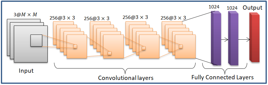
Figure 1 illustrates the proposed deep network architecture for sensor selection. For multi-layer network, the non-linear function $\Sigma(\cdot)$ is represented by the inner layers as

where the first layer $f^{(1)}$ is the input layer and $f^{(i)}_{i\in\{2,4,6,8\}}$ denote the convolutional layers, each of which has 256 filters of size $3\times 3$. The arithmetic operation of a single filter of a convolutional layer is defined for an arbitrary input $\bar{\bf X}\in\mathbb{R}^{d_{x}\times d_{x}\times V_{x}}$ and output $\bar{\bf Y}\in\mathbb{R}^{d_{y}\times d_{y}\times V_{y}}$ as

where $d_{x}\times d_{y}$ is the size of the convolutional kernel, $V_{x}\times V_{y}$ is the size of the response of a convolutional layer, $\bar{\bf W}_{v_{y},v_{k}}\in\mathbb{R}^{V_{x}}$ denotes the weights of the $v_{y}$-th convolutional kernel, and $\bar{\bf X}_{p_{x}}\in\mathbb{R}^{V_{x}}$ is the input feature map at spatial position $p_{x}$. Hence, we define $p_{x}$ and $p_{k}$ as the two-dimensional (2-D) spatial positions in the feature maps and convolutional kernels, respectively [42].

The $10$-th and $12$-th layer are fully connected with 1024 units whose $50\%$ is randomly selected during training to avoid overfitting. A fully connected layer maps an arbitrary input $\bar{\bf x}\in\mathbb{R}^{U_{x}}$ to the output $\bar{\bf y}\in\mathbb{R}^{U_{y}}$ by using the weights $\bar{\bf W}\in\mathbb{R}^{U_{x}\times U_{y}}$. Then, the $u_{y}$-th element of the output of the layer is the inner product

for $u_{y}=1,\dots,U_{y}$ and $\bar{\bf W}_{u_{y}}$ is the $u_{y}$-th column vector of $\bar{\bf W}$, and $U_{x}=U_{y}=1024$ is selected for $f^{(14)}$.

After each convolutional and fully connected layers (i.e., $f^{(i)}_{i\in\{3,5,7,9,11,13\}}$), there is a rectified linear unit ($\mathrm{ReLU}$) layer where $\mathrm{ReLU}(x)=\max(0,x)$. The $\mathrm{ReLU}$ layers are powerful in constructing the non-linearity of the deep network as well as providing non-negative output at the output layers, which is very useful for classification networks. The $14$-th layer has a classification layer with $\bar{C}$ units, where a $\mathrm{softmax}$ function is used to obtain the probability distribution of the classes. The $\mathrm{softmax}$ layer is defined for an arbitrary input $\bar{\mathbf{x}}\in\mathbb{R}^{D}$ as $\mathrm{softmax}(\bar{{x}}_{i})=\frac{\exp\{\bar{x}_{i}\}}{\sum_{i=1}^{D}\exp\{\bar{x}_{i}\}}$. The last layer $f^{(15)}$ is the classification layer.

Once $\mathrm{CNN}_{\mathrm{S}}$ (i.e., $\Sigma_{\mathrm{S}}(\cdot)$) is trained with the source domain data, we freeze the weights in the $\{2,4,6,8\}$-th layers (i.e., the convolutional layers) to preserve the sensor selection ability of the deep network before transferring it to the target domain. We construct the TL network such that

where the frozen layers are $\tilde{f}^{(i)}_{i\in\{2,4,6,8\}}$. Algorithm 1 lists these steps of our proposed TL approach.

We realized the proposed TL architecture in MATLAB on a personal computer (PC) with 768-core graphics processing unit (GPU). For training, we used stochastic gradient descent algorithm with momentum $0.9$ and updated the network parameters at learning rate $0.01$ and mini-batch size of $512$. The loss function was the cross-entropy cost

We first present the performance of the proposed CNN approach for the source domain case where different array geometries such as URA and UCA are considered with different array settings. In particular, we consider sensor arrays with half wavelength sensor spacing for both UCA and URA. When $\mathrm{CNN}_{\mathrm{S}}$s are trained for different arrays, we obtained above $90\%$ validation accuracy for the training data in all cases. In the prediction stage, the DoA angles are generated uniformly at random in the interval $\tilde{\Theta}$ so that the DoA angles in the training and prediction are selected from the same distribution. After feeding $\mathrm{CNN}_{\mathrm{S}}$ with these input data, the selected subarrays are obtained from the output for each scenario. Then, the sensor outputs of corresponding subarrays are employed for DoA estimation using MUSIC (MUltiple SIgnal Classification) algorithm [45]. During the simulations in the prediction state, the network is tested for different SNR levels for $J_{T}=100$ Monte Carlo trials. Figure 3 shows the RMSE in DoA estimation, i.e.,

where $\hat{\phi}^{(j)}$ and $\phi$ denote the estimated and true DoA angles, respectively. We compare the DoA estimation performance of $\mathrm{CNN}_{\mathrm{S}}$ with the best subarray that provides the lowest CRB. Figure 3 demonstrates that $\mathrm{CNN}_{\mathrm{S}}$ asymptotically follows the best subarray performance.

In order to evaluate the TL performance, we trained $\mathrm{CNN}_{\mathrm{S}}$ with different sizes of datasets and then constructed $\mathrm{CNN}_{\mathrm{TR}}$ from $\mathrm{CNN}_{\mathrm{S}}$ for sensor selection. We considered URA and UCA geometries with $M=16$, $K=6$ for source and target domains, respectively. Fig. 4 shows the sensor selection accuracy

where V is the total number of input datasets in which the model identified the best subarrays correctly U times. In Fig. 4(a), the target domain $\mathcal{D}_{\mathrm{T}}$ are generated for $P_{\mathrm{T}}=10$ grid points in $\widetilde{\Theta}$ and $L_{\mathrm{T}}=10$ and we varied $P_{\mathrm{S}}$ from $5$ to $150$ for $\mathcal{D}_{\mathrm{S}}$ with $L_{\mathrm{S}}=100$. For all three networks, The performance of $\mathrm{CNN}_{\mathrm{T}}$ is fixed because $\mathcal{D}_{\mathrm{T}}$ does not change during the simulations. When $P_{\mathrm{S}}$ is very small (i.e., $<10$), $\mathrm{CNN}_{\mathrm{TR}}$ performs even worse than $\mathrm{CNN}_{\mathrm{T}}$. However, as $P_{\mathrm{S}}$ increases, $\mathrm{CNN}_{\mathrm{TR}}$ and $\mathrm{CNN}_{\mathrm{S}}$ exhibit higher selection accuracy. For large source datasets, e.g. $P_{\mathrm{S}}\in[80,120]$, $\mathrm{CNN}_{\mathrm{TR}}$ outperforms $\mathrm{CNN}_{\mathrm{T}}$ by a large margin because of the learned and transferred features from $\mathrm{CNN}_{\mathrm{S}}$. The increase in $P_{\mathrm{S}}$ does not necessarily improve the sensor selection performance because when the training data are densely sampled (i.e., $P_{\mathrm{S}}$ is high) the deep network cannot distinguish the input data of different directions and produce inaccurate classification output. These results suggest that $\mathrm{CNN}_{\mathrm{S}}$ needs to be trained with at least $\textsf{S}=P_{\mathrm{S}}L_{\mathrm{S}}=40\cdot 100=4000$ to provide satisfactory accuracy (e.g., above $90\%$). As a result, $P_{\mathrm{S}}=100$ is a reasonable choice for TL, wherein the target dataset $1000$ times smaller, i.e., $\frac{\textsf{S}}{\textsf{T}}=\frac{L_{\mathrm{S}}P_{\mathrm{S}}}{L_{\mathrm{T}}P_{\mathrm{T}}}=1000$. In Fig. 4(b), we repeat the same analysis for $\mathrm{CNN}_{\mathrm{T}}$ where we assume that $\mathrm{CNN}_{\mathrm{S}}$ is well-trained with $P_{\mathrm{S}}=100$ and $L_{\mathrm{S}}=100$. Then, we sweep $P_{\mathrm{T}}$ similarly for both $L_{\mathrm{T}}=10$ and $L_{\mathrm{T}}=100$. We can see that when $L_{\mathrm{T}}=100$, $\mathrm{CNN}_{\mathrm{T}}$ quickly reaches maximum similar to $\mathrm{CNN}_{\mathrm{S}}$ as illustrated in Fig. 4(a). In this case, the improvement gained by TL is incremental because $\mathrm{CNN}_{\mathrm{T}}$ is already well-trained. However, if small dataset is used, i.e., $L_{\mathrm{T}}=10$, then it requires larger $P_{\mathrm{T}}$ to reach high accuracy. Expectedly, this analysis shows that TL provides reasonable improvement if the target dataset is relatively small, i.e., $\textsf{T}=P_{\mathrm{T}}L_{\mathrm{T}}\leq 1000$ ($\textsf{S}=10000$). In other words, when T is high there is no need to use TL. Therefore, in the following experiments, we select $P_{\mathrm{T}}=L_{\mathrm{T}}=10$ and employ TL to improve the performance.

Table II lists the validation accuracy of $\mathrm{CNN}_{\mathrm{T}}$ and $\mathrm{CNN}_{\mathrm{TR}}$ for different TL scenarios. We consider TL between UCA and URA as well as the perturbed array geometries denoted by $\overline{\mathrm{UCA}}$ and $\overline{\mathrm{URA}}$. In a perturbed array geometry, the $m$-th sensor position is selected uniformly at random as $\{\tilde{x}_{m},\tilde{y}_{m},\tilde{z}_{m}\}\sim\mathcal{N}(\{x_{m},y_{m},z_{m}\},(\lambda/4)^{2})$ for each instance of the training data. It is evident that the sensor selection accuracy of $\mathrm{CNN}_{\mathrm{TR}}$ is approximately $20\%$ higher than $\mathrm{CNN}_{\mathrm{T}}$.

We further assessed the DoA estimation performance of the selected subarrays for target domain data. For $M=16$, $K=6$, Figs. 5 and 6 depict the performance for URA$\rightarrow$UCA and UCA$\rightarrow$URA scenarios, respectively. We compared the sensor selection performance of $\mathrm{CNN}_{\mathrm{T}}$ and $\mathrm{CNN}_{\mathrm{TR}}$ with greedy-based antenna selection (GAS) [19], random selection (RAS) as well as the fully array performance. As expected, we see that the full array has the lowest SNR due to large array aperture. We observe that $\mathrm{CNN}_{\mathrm{TR}}$ closely follows the performance of the best subarray. The $\mathrm{CNN}_{\mathrm{TR}}$ exhibits approximately $4\%$, $8.5\%$ and $23\%$ lower RMSE as compared to GAS, $\mathrm{CNN}_{\mathrm{T}}$ and RAS, respectively. It is worth noting that RAS has no rule on selecting the antennas while GAS is a greedy-based suboptimum method seeking the best subarray based on the CRB information [19]. These results establish the effectiveness of TL for DoA estimation with sensor selection. The superior performance of $\mathrm{CNN}_{\mathrm{TR}}$ is because of the learned and transferred features from source domain data via $\mathrm{CNN}_{\mathrm{S}}$.

In practical applications, the deployment of sensor arrays is a one-time operation. When the physical conditions around the sensor array change, the positions of the sensors are often slightly altered. Over longer duration, the position of the sensors become different from the ones when the array is installed. In this experiment, we show that our TL approach for sensor arrays performs well even when the sensor positions are perturbed. Figures 7 and 8 show the DoA estimation RMSE for URA and UCA, respectively. The target array geometry has been perturbed with $\lambda/4$ standard deviation in sensor positions (see Section V-B). The proposed TL approach clearly results in lesser estimation error than $\mathrm{CNN}_{\mathrm{T}}$. In particular, $\mathrm{CNN}_{\mathrm{TR}}$ produces approximately $4\%$, $10\%$, and $28\%$ lower RMSE than GAS, $\mathrm{CNN}_{\mathrm{T}}$, and RAS, respectively.

We assessed the performance of TL when the target data is corrupted. We used the settings of Fig. 5, i.e., URA $\rightarrow$ UCA for $M=16$, $K=6$. The target sensor data is corrupted by mutual coupling (MC). The received signal now becomes [37]

where $\mathbf{C}\in\mathbb{C}^{M\times M}$ is a Hermitian Toeplitz MC matrix, which for a UCA is $\mathbf{C}=\mathrm{Toeplitz}\{c_{1},c_{2},\dots,c_{L},c_{L-1},\dots,c_{2}\}$. Here $\{c_{l}\}_{l=1}^{L}$ are the MC coefficients and $L=\frac{M}{2}+1$ for even $M$. Let $\mathbf{c}=[c_{1},\dots,c_{L}]^{T}$ be the MC coefficient vector, then we model $\mathbf{c}$ such that $c_{1}=1$ and $c_{l}=0.6\big(1-\frac{(l-2)}{L-1}\big)e^{j\varphi_{l}}$ for $l=2,\dots,L$ where $\varphi_{l}\in[-\pi,\pi]$ is a random phase information. This yields that the magnitude of the coupling coefficient for the closest and furthest sensor pairs are $c_{2}=0.6$ and $c_{L}=0.075$, respectively [46]. To investigate the effect of MC, define $\mathbf{c}=\gamma[1/\gamma,c_{2},\dots,c_{L}]^{T}$ and sweep $\gamma$ as $\gamma\in[0.01,1]$. The resulting performance in Fig. 9 shows that the performance of all algorithms degrades as $\gamma\rightarrow 1$, i.e., the effect of MC becomes stronger. $\mathrm{CNN}_{\mathrm{TR}}$ performs better than $\mathrm{CNN}_{\mathrm{T}}$ as long as $\gamma\leq 0.6$ because the corrupted data becomes unfamiliar to $\mathrm{CNN}_{\mathrm{TR}}$ and it yields worse RMSE than $\mathrm{CNN}_{\mathrm{T}}$ and GAS.

So far, we restricted our experiments to a fixed elevation angle. Figure 10 shows the 2-D DoA estimation performance for the UCA$\rightarrow$URA scenario. In source domain, we selected $P_{\mathrm{S}}=11000$ where the azimuth plane is sampled with $P_{{\phi}_{\mathrm{S}}}=100$ and the elevation plane is sampled uniformly with $P_{{\theta}_{\mathrm{S}}}=11$ in the sector $[80^{\circ},90^{\circ}]$. In target domain, we selected $P_{\mathrm{T}}=600$ ($\sim 5\%$ of $P_{\mathrm{S}}$) where $P_{{\theta}_{\mathrm{T}}}=6$ and $P_{{\phi}_{\mathrm{T}}}=10$. In this experiment, we consider different $K$ values, namely, $K_{\mathrm{S}}=6$ and $K_{\mathrm{T}}=8$. The number of snapshots are $T=10$. The RMSE is calculated for the joint estimation of $\theta$ and $\phi$. For 2-D scenario, the results are similar to the 1-D case: $\mathrm{CNN}_{\mathrm{TR}}$ has $7\%$, $20\%$, and $38\%$ lower RMSE than GAS, $\mathrm{CNN}_{\mathrm{T}}$, and RAS, respectively. Note that the RMSE for all algorithms is high (approximately $70^{\circ}$ for $\mathrm{SNR}=0$ dB) because of the small array aperture in vertical dimension [46].

Since all deep networks have the same architecture, $\mathrm{CNN}_{\mathrm{S}}$, $\mathrm{CNN}_{\mathrm{T}}$ and $\mathrm{CNN}_{\mathrm{TR}}$ have the same complexity. For a deep neural network with $L_{\mathrm{C}}$ convolutional layers, the time complexity is [47]

where $D_{x}^{(l)},D_{y}^{(l)}$ are the column and row sizes of each output feature map, $b_{x}^{(l)},b_{y}^{(l)}$ are the 2D filter size of the $l$-th layer. $N_{\mathrm{CL}}^{(l-1)}$ and $N_{\mathrm{CL}}^{(l)}$ denote the number of input and output feature maps of the $l$-th layer respectively. In Table III, we have shown the parameters of each convolutional layer. Thus, the complexity of $4$ convolutional layers with $256$@$3\times 3$ filters approximately becomes

The time complexity of $L_{\mathrm{F}}$ fully connected layers similarly is

where $N_{\mathrm{FCL}}^{(l)}$ is the number of units of $l$-th fully connected layer and $D_{1}^{(l)},D_{2}^{(l)}$ are the 2D input size of the $l$-th fully connected layer and $N_{\mathrm{FCL}}^{(l)}$ is the number of units, each of which has $50\%$ dropout. Table IV lists the parameters of fully connected layers whose complexity approximately is

Hence the total time complexity of the DL approach is $\mathcal{C}=\mathcal{C}_{\mathrm{CL}}+\mathcal{C}_{\mathrm{FCL}}$ which is approximately

which is further simplified as $\approx\mathcal{O}\big(38\cdot 256^{2}M^{2}\big)$. In comparison, the order of an analytical approach such as GAS is $\mathcal{O}\big(KM^{2}\big)$ [19]. The RAS has sorting complexity of $\mathcal{O}\big(M\log M\big)$ [18] at the cost of performance. While the complexity of CNN is on the order of magnitude of $10^{6}$, it is able to run in more efficient parallel manner by using GPUs, whereas the other algorithms cannot be implemented in such a way easily. The computation time of the proposed CNN approach only takes about $10\times 10^{-3}$ s for $M=16$ and $K=6$, whereas RAS and GAS need approximately $30\times 10^{-3}$ and $130\times 10^{-3}$, respectively. Similar observations about the fast computation times of the DL networks have been reported in [47, 48, 21, 49].

References

- [1] R. P. Shenoy, “Phased array antennas,” in Advanced radar techniques and systems (G. Galati, ed.), Peter Peregrinus, 1993.
- [2] J. Frank and J. D. Richards, “Phased array radar antennas,” in Radar handbook (M. I. Skolnik, ed.), McGraw-Hill Education, third ed., 2008.
- [3] J. S. Herd and M. D. Conway, “The evolution to modern phased array architectures,” Proceedings of the IEEE, vol. 104, no. 3, pp. 519–529, 2015.
- [4] R. L. Haupt, Timed Arrays: Wideband and Time Varying Antenna Arrays. John Wiley & Sons, 2015.
- [5] D. H. Johnson, “The application of spectral estimation methods to bearing estimation problems,” Proceedings of the IEEE, vol. 70, no. 9, pp. 1018–1028, 1982.
- [6] D. A. Linebarger, I. H. Sudborough, and I. G. Tollis, “Difference bases and sparse sensor arrays,” IEEE Transactions on information theory, vol. 39, no. 2, pp. 716–721, 1993.
- [7] R. L. Haupt, “Thinned arrays using genetic algorithms,” IEEE Transactions on Antennas and Propagation, vol. 42, no. 7, pp. 993–999, 1994.
- [8] X. Wang, Z. Chen, S. Ren, and S. Cao, “DOA estimation based on the difference and sum coarray for coprime arrays,” Digital Signal Processing, vol. 69, pp. 22 – 31, 2017.
- [9] K. V. Mishra, I. Kahane, A. Kaufmann, and Y. C. Eldar, “High spatial resolution radar using thinned arrays,” in IEEE Radar Conference, pp. 1119–1124, 2017.
- [10] S. S., M. R. Bhavani Shankar, K. V. Mishra, and B. Ottersten, “Optimum design for sparse FDA-MIMO automotive radar,” in Asilomar Conference on Signals, Systems, and Computers, 2019. in press.
- [11] E. BouDaher, F. Ahmad, M. G. Amin, and A. Hoorfar, “Mutual coupling effect and compensation in non-uniform arrays for direction-of-arrival estimation,” Digital Signal Processing, vol. 61, pp. 3–14, 2017.
- [12] C. L. Liu and P. P. Vaidyanathan, “Super Nested Arrays: Linear Sparse Arrays With Reduced Mutual Coupling; Part I: Fundamentals,” IEEE Transactions on Signal Processing, vol. 64, pp. 3997–4012, Aug 2016.
- [13] C.-L. Liu and P. P. Vaidyanathan, “Hourglass arrays and other novel 2-D sparse arrays with reduced mutual coupling,” IEEE Transactions on Signal Processing, vol. 65, no. 13, pp. 3369–3383, 2017.
- [14] A. M. Elbir and K. V. Mishra, “Joint antenna selection and hybrid beamformer design using unquantized and quantized deep learning networks,” IEEE Trans. Wireless Commun., vol. 19, no. 3, pp. 1677–1688, 2020.
- [15] A. Moffet, “Minimum-redundancy linear arrays,” IEEE Transactions on antennas and propagation, vol. 16, no. 2, pp. 172–175, 1968.
- [16] R. J. Kozick and S. A. Kassam, “Linear imaging with sensor arrays on convex polygonal boundaries,” IEEE Transactions on Systems, Man, and Cybernetics, vol. 21, no. 5, pp. 1155–1166, 1991.
- [17] T. M. Duman and A. Ghrayeb, “Antenna selection for MIMO systems,” in Coding for MIMO Communication Systems, pp. 287–315, John Wiley & Sons, 2007.
- [18] S. Joshi and S. Boyd, “Sensor selection via convex optimization,” IEEE Transactions on Signal Processing, vol. 57, no. 2, pp. 451–462, 2009.
- [19] H. Godrich, A. P. Petropulu, and H. V. Poor, “Sensor selection in distributed multiple-radar architectures for localization: A knapsack problem formulation,” IEEE Transactions on Signal Processing, vol. 60, no. 1, pp. 247–260, 2012.
- [20] A. M. Elbir and K. V. Mishra, “Robust hybrid beamforming with quantized deep neural networks,” in IEEE International Workshop on Machine Learning for Signal Processing, pp. 1–6, 2019.
- [21] A. M. Elbir, K. V. Mishra, and Y. C. Eldar, “Cognitive radar antenna selection via deep learning,” IET Radar, Sonar & Navigation, vol. 13, pp. 871–880, 2019.
- [22] D. Yu and L. Deng, “Deep learning and its applications to signal and information processing [exploratory dsp],” IEEE Signal Processing Magazine, vol. 28, no. 1, pp. 145–154, 2011.
- [23] A. M. Elbir and K. V. Mishra, “Deep learning design for joint antenna selection and hybrid beamforming in massive MIMO,” in IEEE International Symposium on Antennas and Propagation and USNC-URSI Radio Science Meeting, pp. 1585–1586, 2019.
- [24] A. M. Elbir and K. V. Mishra, “Online and offline deep learning strategies for channel estimation and hybrid beamforming in multi-carrier mm-Wave massive MIMO systems,” arXiv preprint arXiv:1912.10036v2, 2020.
- [25] A. M. Elbir and K. V. Mishra, “Low-complexity limited-feedback deep hybrid beamforming for broadband massive MIMO communications,” in IEEE International Workshop on Signal Processing Advances in Wireless Communications, 2020. in press.
- [26] L. Duan, I. W. Tsang, and D. Xu, “Domain transfer multiple kernel learning,” IEEE Transactions on Pattern Analysis and Machine Intelligence, vol. 34, no. 3, pp. 465–479, 2012.
- [27] B. Kulis, K. Saenko, and T. Darrell, “What you saw is not what you get: Domain adaptation using asymmetric kernel transforms,” in IEEE Conference on Computer Vision and Pattern Recognition, pp. 1785–1792, 2011.
- [28] S. J. Pan, Q. Yang, et al., “A survey on transfer learning,” IEEE Transactions on Knowledge and Data Engineering, vol. 22, no. 10, pp. 1345–1359, 2010.
- [29] P. Vincent, H. Larochelle, I. Lajoie, Y. Bengio, and P.-A. Manzagol, “Stacked denoising autoencoders: Learning useful representations in a deep network with a local denoising criterion,” Journal of machine learning research, vol. 11, no. Dec, pp. 3371–3408, 2010.
- [30] M. S. Seyfioğlu and S. Z. Gürbüz, “Deep neural network initialization methods for micro-Doppler classification with low training sample support,” IEEE Geoscience and Remote Sensing Letters, vol. 14, no. 12, pp. 2462–2466, 2017.
- [31] B. Chen, Z. Zhong, B. Ai, and X. Chen, “Comparison of antenna arrays for mimo system in high speed mobile scenarios,” in 2011 IEEE 73rd Vehicular Technology Conference (VTC Spring), pp. 1–5, 2011.
- [32] P. Hyberg, M. Jansson, and B. Ottersten, “Array interpolation and bias reduction,” IEEE Transactions on Signal Processing, vol. 52, no. 10, pp. 2711–2720, 2004.
- [33] M. Rubsamen and A. B. Gershman, “Direction-of-arrival estimation for nonuniform sensor arrays: From manifold separation to Fourier domain MUSIC methods,” IEEE Transactions on Signal Processing, vol. 57, no. 2, pp. 588–599, 2008.
- [34] Y. Liu, H. Chen, Z. Peng, and J. Fang, “DOA estimation for mixed circular and noncircular signals by using the conversion relationship between URAs and a virtual ULA,” IEEE Sensors Letters, vol. 3, no. 11, pp. 1–4, 2019.
- [35] Z.-M. Liu, C. Zhang, and S. Y. Philip, “Direction-of-arrival estimation based on deep neural networks with robustness to array imperfections,” IEEE Transactions on Antennas and Propagation, vol. 66, no. 12, pp. 7315–7327, 2018.
- [36] P. Stoica and A. Nehorai, “MUSIC, maximum likelihood, and Cramér-Rao bound: Further results and comparisons,” IEEE Transactions on Acoustics, Speech, and Signal Processing, vol. 38, no. 12, pp. 2140–2150, 1990.
- [37] B. Friedlander and A. Weiss, “Direction finding in the presence of mutual coupling,” IEEE Transactions on Antennas and Propagation, vol. 39, no. 3, pp. 273–284, 1991.
- [38] A. M. Elbir, S. Mulleti, R. Cohen, R. Fu, and Y. C. Eldar, “Deep-sparse array cognitive radar,” in IEEE International Conference on Sampling Theory and Applications, pp. 1–5, 2019.
- [39] A. Renaux, P. Forster, P. Larzabal, C. D. Richmond, and A. Nehorai, “A fresh look at the Bayesian bounds of the Weiss-Weinstein family,” IEEE Transactions on Signal Processing, vol. 56, no. 11, pp. 5334–5352, 2008.
- [40] D. Nion and N. D. Sidiropoulos, “Tensor algebra and multidimensional harmonic retrieval in signal processing for MIMO radar,” IEEE Transactions on Signal Processing, vol. 58, no. 11, pp. 5693–5705, 2010.
- [41] Z. Ye and C. Liu, “2-D DOA estimation in the presence of mutual coupling,” IEEE Transactions on Antennas and Propagation, vol. 56, no. 10, pp. 3150–3158, 2008.
- [42] J. Cheng, J. Wu, C. Leng, Y. Wang, and Q. Hu, “Quantized CNN: A unified approach to accelerate and compress convolutional networks,” IEEE Transactions on Neural Networks and Learning Systems, vol. 29, no. 10, pp. 4730–4743, 2018.
- [43] S. J. Pan, I. W. Tsang, J. T. Kwok, and Q. Yang, “Domain adaptation via transfer component analysis,” IEEE Transactions on Neural Networks, vol. 22, no. 2, pp. 199–210, 2010.
- [44] J. Yosinski, J. Clune, Y. Bengio, and H. Lipson, “How transferable are features in deep neural networks?,” in Advances in neural information processing systems, pp. 3320–3328, 2014.
- [45] R. Schmidt, “Multiple emitter location and signal parameter estimation,” IEEE Transactions on Antennas and Propagation, vol. 34, no. 3, pp. 276–280, 1986.
- [46] A. M. Elbir, “A novel data transformation approach for doa estimation with 3-d antenna arrays in the presence of mutual coupling,” IEEE Antennas Wireless Propag. Lett., vol. 16, pp. 2118–2121, 2017.
- [47] K. Simonyan and A. Zisserman, “Very deep convolutional networks for large-scale image recognition,” arXiv preprint arXiv:1409.1556, 2014.
- [48] P. Dong, H. Zhang, G. Y. Li, I. S. Gaspar, and N. NaderiAlizadeh, “Deep CNN-Based Channel Estimation for mmWave Massive MIMO Systems,” IEEE J. Sel. Areas Commun., vol. 13, pp. 989–1000, Sep. 2019.
- [49] A. M. Elbir, “DeepMUSIC: Multiple Signal Classification via Deep Learning,” IEEE Sensors Letters, vol. 4, no. 4, pp. 1–4, 2020.
![[Uncaptioned image]](2004.11637v2/elbirPhoto.jpg) |
Ahmet M. Elbir [S’13–M’16–SM’20] received the B.S. degree with Honors from Firat University in 2009 and the Ph.D. degree from Middle East Technical University (METU) in 2016, both in electrical engineering. He is the recipient of 2016 METU best Ph.D. thesis award for his doctoral studies. He serves as an Associate Editor for IEEE Access since 2018. Currently, he is a visiting postdoctoral researcher at Koc University, Istanbul, Turkey. His research interests include array signal processing, sparsity-driven convex optimization, signal processing for communications and deep learning for array signal processing. |
![[Uncaptioned image]](2004.11637v2/kvm_taes.jpg) |
Kumar Vijay Mishra [S’08–M’15–SM’18] received B.Tech., summa cum laude (Gold medal, honors), in electronics and communications engineering from the National Institute of Technology, Hamirpur, India, in 2003, M.S. in electrical and computer engineering from Colorado State University, Fort Collins, in 2012, and his Ph.D. degree in electrical and computer engineering and M.S. degree in mathematics from The University of Iowa, Iowa City, in 2015 while working on NASA Global Precipitation Mission Ground Validation program weather radars. He is the recipient of IEEE MLSP Best Paper Award (2019), Royal Meteorological Society Quarterly Journal Editor’s Prize (2017), Andrew and Erna Finci Viterbi Postdoctoral Fellowship (2015 and 2016), and Lady Davis Postdoctoral Fellowship (2016). Currently, he is visiting scholar at The University of Iowa; Research Fellow at the University of Luxembourg; and National Academies Harry Diamond Distinguished Fellow at the U. S. Army Research Laboratory. His research interests include remote sensing, signal processing, communications, deep learning, and electromagnetics. |